Decay of the Fourier transform of surfaces with
vanishing curvature

Abstract

We prove $L^{p}$-bounds on the Fourier transform of measures $\mu$ supported on two dimensional surfaces. Our method allows to consider surfaces whose Gauss curvature vanishes on a one-dimensional submanifold. Under a certain non-degeneracy condition, we prove that $\widehat{\mu}\in L^{4+\beta}$, $\beta>0$, and we give a logarithmically divergent bound on the $L^{4}$-norm. We use this latter bound to estimate almost singular integrals involving the dispersion relation, $e(p)=\sum_{1}^{3}[1-\cos p_{j}]$, of the discrete Laplace operator on the cubic lattice. We briefly explain our motivation for this bound originating in the theory of random Schrödinger operators.

AMS 2000 Subject Classification: 42B10, 81T18

1 Introduction

1.1 Notations and background

Let $\Sigma$ be a smooth, compact hypersurface embedded in ${\mathbb{R}}^{3}$ or in the torus ${\bf T}^{3}=[-\pi,\pi]^{3}$. Let ${\rm d}m$ be the induced surface area measure on $\Sigma$ and let $f\in C_{0}^{\infty}(\Sigma)$, i.e. $f$ is a smooth function supported away from the boundary of $\Sigma$. Let $\kappa_{i}=\kappa_{i}(p)$, $i=1,2$, denote the two principal curvatures at $p\in\Sigma$, let $K=\kappa_{1}\kappa_{2}$ be the Gauss curvature and $H=\kappa_{1}+\kappa_{2}$ the mean curvature.

We define the Fourier transform of the measure ${\rm d}\mu=f{\rm d}m$,

$$\widehat{\mu}(\xi)=\int_{\Sigma}e^{i\xi\cdot p}f(p){\rm d}m(p)\;,\qquad\xi\in{\mathbb{R}}^{3},$$ (1.1)

and we investigate the decay properties of $\widehat{\mu}$ at infinity. We prove that

$$\widehat{\mu}\in L^{4+\beta}({\mathbb{R}}^{3}),\qquad\beta>0\;,$$ (1.2)

and

$$J_{\eta}=\int_{|\xi|\leq\eta^{-1}}|\widehat{\mu}(\xi)|^{4}{\rm d}\xi\leq C|\log\eta|^{10},$$ (1.3)

with some constant $C$ depending only on $f$ and on a few geometric properties of the surface $\Sigma$. The estimate (1.3) indicates a decay $\widehat{\mu}(\xi)\lesssim\langle\xi\rangle^{-3/4}$, with $\langle\xi\rangle=(\xi^{2}+1)^{1/2}$, for almost all $\xi$.

By a standard stationary phase argument (see, e.g., Theorem 1, Section VIII.3.1 of [13]) it is well known that the decay estimate

$$|\widehat{\mu}(\xi)|\leq\frac{C}{\langle\xi\rangle^{r}}$$ (1.4)

holds with $r=1$ if $K$ nowhere vanishes on the support of $f$. The constant depends on the lower bound on $|K|$ and on supremum bounds of a few derivatives of $f$. In particular, this bound holds for uniformly convex surfaces.

Fewer results are available if $K$ is allowed to vanish. In the extreme case, when $K\equiv 0$ and $\Sigma$ is flat, $\widehat{\mu}(\xi)$ does not decay in the direction orthogonal to $\Sigma$. In the general case, local results can easily be obtained by a stationary phase analysis. To formulate them, let $\nu(p)$ denote the unit normal at the point $p\in\Sigma$. Assume that $f$ is supported in a sufficiently small neighborhood ${\cal U}$ of $p$. Then the rate of decay of $|\widehat{\mu}(\lambda\nu(p))|$ for $|\lambda|\gg 1$ is estimated as

$$|\widehat{\mu}(\lambda\nu(p))|\leq C|\lambda|^{-k/2},\qquad|\lambda|\gg 1,$$ (1.5)

where $k$ is the number of nonvanishing principal curvatures at $p$ (see e.g. Section VIII.5.8 of [13]). The constant in this estimate depends on the point $p$ unless a uniform lower bound is known on the non-vanishing curvatures. For example, (1.4) holds with a uniform constant and with $r=1/2$ if $|\kappa_{1}|+|\kappa_{2}|\geq c_{0}>0$ on the support of $f$. For vectors $\xi$ that are not parallel with any normal vector $\nu(p)$, $p\in{\cal U}$, the decay rate is polynomial with arbitrary high degree,

$$|\widehat{\mu}(\xi)|\leq C|\xi|^{-N},\qquad N\in{\bf N}\;.$$ (1.6)

Here the constant depends on $N$ and on $\inf\{|\nu(p)\times{\omega}_{\xi}|\;:\;p\in{\cal U}\}$ with ${\omega}_{\xi}=\xi/|\xi|$, where $\times$ denotes the cross product.

To obtain an $L^{p}$-bound on $\widehat{\mu}$, one must control the behavior of the constants in (1.5) and (1.6) that depend on further geometric properties of $\Sigma$. For a convex hypersurface $\Sigma$, Bruna, Nagel and Wainger [2] have shown that

$$|\widehat{\mu}(\lambda\nu(p))|\leq C\;\mbox{Vol}(\,B(p,\lambda^{-1})\,)\;,$$

where $B(p,h)=\{y\in\Sigma\;:\;(p-y)\cdot\nu(p)\leq h\}$ is the spherical “cap” of height $h$ ($h\ll 1$) around $p$ and $\nu(p)$ is the “outer” normal. One can thus determine the constant in (1.5) by a local Taylor expansion. Iosevich [9] showed that $|B(p,\delta)|\leq C\delta^{r}$ is equivalent to (1.4) for convex hypersurfaces of finite type (i.e. the order of contact with any tangent line is finite). The convexity is essential in these estimates.

Our goal is to prove (1.2) and (1.3) for a class of non-convex hypersurfaces; in particular $K$ will be allowed to vanish on a one-dimensional submanifold of $\Sigma$. We assume that both curvatures cannot vanish at any point, i.e. there is no flat umbilic point on $\Sigma$. By compactness this means

$$|\kappa_{1}|+|\kappa_{2}|\geq(const)>0\;,$$ (1.7)

in particular $|\widehat{\mu}(\xi)|\leq C|\xi|^{-1/2}$ for all $\xi$, and $|\widehat{\mu}(\xi)|\leq C({\omega}_{\xi})|\xi|^{-1}$ (with an ${\omega}_{\xi}$-dependent constant) unless $\xi$ is parallel with a normal vector $\nu(p)$ on the zero set of $K$, i.e. $K(p)=0$. If one naively uses the estimate $|\widehat{\mu}(\xi)|\leq C|\xi|^{-1/2}$ for all $\xi$’s on the two-dimensional submanifold $\{\xi\;:\;\xi\|\nu(p),\;K(p)=0\}\subset{\mathbb{R}}^{3}$ and $|\widehat{\mu}(\xi)|\leq C({\omega}_{\xi})|\xi|^{-1}$ for all other $\xi$, then the integral $J_{\eta}$ diverges as $|\log\eta|$. This indicates that the bound (1.3) is close to optimal for surfaces satisfying (1.7). For the proof, however, we will need further technical non-degeneracy assumptions on $\Sigma$.

Note that this argument is only heuristic since it neglects to control the constant in $|\widehat{\mu}(\xi)|\leq C({\omega}_{\xi})|\xi|^{-1}$. The main technical result (Theorem 2.1) is to give an effective estimate for $|\widehat{\mu}(\xi)|$ that can be integrated to obtain (1.2), (1.3) (Corollary (2.2)).

We mention that the lack of decay due to the vanishing curvature can be mitigated by a curvature factor in the integral. The following general result was obtained by Sogge and Stein [12]

$$\Big{|}\int_{\Sigma}e^{i\xi\cdot p}K(p)^{4}f(p){\rm d}m(p)\Big{|}\leq C\langle\xi\rangle^{-1}$$

for any hypersurface. Similar result holds for hypersurfaces in any dimension.

We also mention that the bound (1.4) with some $r>0$ implies classical Fourier restriction estimates, for example

$$\Big{(}\int_{\Sigma}|\widehat{g}|^{2}{\rm d}\mu\Big{)}^{1/2}\leq C\|g\|_{2(r+1)/(r+2)}\;$$

for any function $g$ on ${\mathbb{R}}^{3}$ [8]. The restriction theorem has been investigated for certain special surfaces with vanishing curvature. Oberlin considers a rotationally symmetric surface with curvature vanishing at one point [11]. Very recently Morii obtained a restriction theorem for surfaces given as graphs of real polynomials that are sums of monomials [10]. It would be interesting to investigate the restriction theorem for the class of hypersurfaces we consider.

The paper is organized as follows. In Section 1.2 we explain our original motivation to study this problem. In Section 2.1 we formulate the assumptions on the surface $\Sigma$ and state our bound on the decay of $|\widehat{\mu}(\xi)|$. As a corollary of this estimate, we will obtain (1.2) and (1.3). In Section 2.2 we formulate a theorem, the so-called Four Denominator Estimate, that is ultimately connected with the $L^{4}$-bound of the Fourier transform of an explicitly given surface. This surface is the level set of the dispersion relation of the discrete Laplace operator (see (2.22) below). Section 3 contains the proof of the bound on $|\widehat{\mu}(\xi)|$. Finally, in Section 4 we prove the Four Denominator Estimate. It will be an easy consequence of our general bound on $|\widehat{\mu}(\xi)|$, once we have checked that the assumptions are satisfied for this particular surface. Despite the explicit formula for the dispersion relation, verifying the otherwise generic assumptions is a non-trivial task.

1.2 Motivation: Random Schrödinger evolution

Although the decay of the Fourier transform of measures supported on hypersurfaces is an interesting and broadly studied problem itself, our motivation to prove the estimate (1.3) came from elsewhere.

We studied the long-time behavior of the random Schrödinger equation

$$i\partial_{t}\psi_{t}(x)=\Big{[}-\frac{1}{2}\Delta_{x}+\lambda V(x)\Big{]}\psi_{t}(x)\;,\qquad\psi_{t}(x)\in L^{2}({\mathbb{R}}^{3}),$$ (1.8)

in the three dimensional Euclidean space, $x\in{\mathbb{R}}^{3}$. Here $V(x)$ is a random potential with a short scale correlation and $\lambda$ is a small coupling constant.

The equation (1.8) models the quantum evolution of an electron in a random impure environment. It has been proved that the electron is localized for sufficiently large $\lambda$. It is conjectured, but not yet proven, that the evolution is delocalized, moreover diffusive for all times, if $\lambda$ is sufficiently small. In [5], [6], jointly with H.-T. Yau we proved a weaker statement, namely we proved diffusion up to time scale $t\sim\lambda^{-2-\kappa}$, $\kappa>0$, in the scaling limit $\lambda\to 0$. For the precise statement, the physical background and references, see [5].

The discrete analogue of (1.8) is the celebrated Anderson model [1]. In this model the electron is hopping on the lattice, $x\in{\mathbb{Z}}^{3}$, generated by the discrete Laplace operator $\Delta_{x}$. The random potential $V(x)$ describes the potential strength of a random obstacle at the location $x$. It is given by a collection of i.i.d. random variables $\{V(x)\;:\;x\in{\mathbb{Z}}^{3}\}$. Since the (de)localization problem concerns large distances, physically there is no difference between the continuous and the discrete model. In fact, the proofs in the localization regime have technically been somewhat simpler for the discrete model since the large momentum regime is not present. Similar simplifications have arisen when we implemented our diffusion result [5], [6] to the discrete setup [7]. However, the lattice formulation gave rise to a seemingly innocent technical difficulty that became an unexpectedly tough problem.

The basic approach of our work on random Schrödinger evolutions is perturbative: we expand the unitary kernel, $e^{-itH}$, of $H=-\frac{1}{2}\Delta+\lambda V$ around the free evolution, $e^{it\Delta/2}$. After taking the expectation with respect to the randomness, the Wigner transform of $\psi_{t}$ is written as a sum over Feynman graphs representing different collision histories. The value of each Feynman graph is a multiple integral of momentum variables $p_{j}\in{\bf T}^{3}$ that are subject to linear constraints. The integrand is a product of functions of the form $(\alpha-e(p_{j})+i\eta)^{-1}$, the so-called time-independent free propagators. Here $\alpha\in{\mathbb{R}}$ and the function $e(p)$ is the Fourier multiplier of $-\frac{1}{2}\Delta$. The regularization $\eta$ is the inverse time, $\eta=t^{-1}\ll 1$.

One of our key steps is to prove that the evolution becomes Markovian as $\lambda\to 0$. If the electron collides with the same random obstacle more than once, then Markovity is violated. We must thus prove that the Feynman graphs with recollision processes have negligible contributions. In the Feynman integral, a double recollision corresponds to a factor

$$\frac{\delta(p-q+r-v)\;{\rm d}p{\rm d}q{\rm d}r{\rm d}v}{(\alpha-e(p)+i\eta)(\alpha-e(q)+i\eta)(\alpha-e(r)+i\eta)(\alpha-e(v)+i\eta)}\;,$$ (1.9)

where $p,q$ and $r,v$ are the pre- and postcollision velocities in the first and second collisions with the same obstacle. The delta function expresses a natural momentum conservation (for more details on Feynman graphs, see [7]). It is therefore necessary to give a good estimate for the integral of these four denominators connected with a delta function. This will be our Four Denominator Estimate formulated in Theorem 2.4.

Acknowledgement. This work is part of a joint project with H.-T. Yau on quantum diffusion. The authors express their gratitude for his discussions and comments on this work . The authors are also indebted to A. Szűcs for helpful discussions.

2 Statement of the main results

2.1 Theorems on the decay of the Fourier transform.

In this section we formulate the geometric assumptions and we state a general theorem on the decay of the Fourier transform of measures supported on surfaces. First we discuss the case of a family of surfaces that is represented as level sets of a regular function. Then we explain how this result can be used to investigate the case of a single surface.

Let $e(p)$ be a smooth real function on ${\mathbb{R}}^{3}$ or ${\bf T}^{3}=[-\pi,\pi]^{3}$ and let $\Sigma_{a}=\{p\;:\;e(p)=a\}$ be the $a$-level set for any $a\in{\mathbb{R}}$. Let ${\cal I}\subset{\mathbb{R}}$ be a finite union of compact intervals such that the preimage ${\cal D}=e^{-1}({\cal I})$ is compact and $\Sigma_{a}$ is a two-dimensional submanifold for each $a\in{\cal I}$. Let $f$ be a smooth function on ${\cal D}$, and define

$$\widehat{\mu}_{a}(\xi)=\int_{\Sigma_{a}}e^{i\xi\cdot p}f(p){\rm d}m_{a}(p)\;,$$ (2.1)

the Fourier transform of the measure $f{\rm d}m_{a}$, where ${\rm d}m_{a}$ is the induced surface area measure on $\Sigma_{a}$.

We define

$$C_{0}=\mbox{diam}({\cal D}),\qquad C_{1}=\|e\|_{C^{5}({\cal D})}\;.$$ (2.2)

We set the following

$$\mbox{\bf Assumption 1:}\qquad C_{2}=\min_{{\cal D}}|\nabla e|>0\;,\qquad\qquad\qquad$$ (2.3)

i.e. we require that the level surfaces $\Sigma_{a}$, $a\in{\cal I}$, form a regular foliation of ${\cal D}$. In particular, $\Sigma_{a}$ has no boundary.

Let $K:{\cal D}\to{\mathbb{R}}$ be the Gauss curvature of the foliation, i.e. $K(p)$ is the Gauss curvature of $\Sigma_{a}$ at $p$ if $p\in\Sigma_{a}$. Since $K$ is the determinant of the second fundamental form of a smooth foliation, it is a smooth function on ${\cal D}$.

We also assume that the zero set of the Gauss curvature intersects the foliation $(\Sigma_{a})_{a\in{\cal I}}$ transversally:

Assumption 2. Let ${\cal G}=\{p\in{\cal D}\;:\;K(p)=0\}$. Then

$$C_{3}=\min\big{\{}|\nabla e(p)\times\nabla K(p)|\;:\;p\in{\cal G}\big{\}}>0\;.$$ (2.4)

This implies in particular that $\nabla K$ does not vanish on ${\cal G}$, so ${\cal G}$ is a two-dimensional submanifold of ${\cal D}$, and the two principal curvatures $\kappa_{1}(p)$, $\kappa_{2}(p)$ cannot vanish simultaneously, i.e. there is no flat umbilic point. By compactness,

$$\underline{\kappa}=\min_{\cal D}\;(|\kappa_{1}|+|\kappa_{2}|)>0\;$$ (2.5)

and $\underline{\kappa}$ depends only on $C_{0},C_{1},C_{2},C_{3}$. Since $e(p)$ and $K(p)$ are smooth, it follows from (2.4) that the zero curvature set,

$$\Gamma_{a}={\cal G}\cap\Sigma_{a}$$

is a finite union of disjoint regular curves on $\Sigma_{a}$ for each $a\in{\cal I}$. All these curves are simple and closed. Let

$$p\mapsto w(p)=\frac{\nabla e(p)\times\nabla K(p)}{|\nabla e(p)\times\nabla K(p)|}\;$$ (2.6)

be the unit vectorfield tangent to $\Gamma_{a}$.

Define the normal map $\nu:{\cal D}\to S^{2}$, given by

$$\nu(p)=\frac{\nabla e(p)}{|\nabla e(p)|}\;.$$ (2.7)

The Jacobian of the normal map restricted to each surface, $\nu:\Sigma_{a}\to S^{2}$, is the Gauss curvature, $\mbox{det}\;\nu^{\prime}(p)=K(p)$.

Assumption 3. The number of preimages of $\nu:\Sigma_{a}\to S^{2}$ is finite, i.e.

$$C_{4}=\sup_{a\in{\cal I}}\sup_{{\omega}\in S^{2}}\mbox{card}\{p\in\Sigma_{a}\;:\;\nu(p)={\omega}\}<\infty\;.$$ (2.8)

On the (union of) curves $\Gamma_{a}$, exactly one of the principal curvatures vanish, hence the principal direction of the zero curvature is well defined. This defines a (local) unit vectorfield $Z\in T\Sigma_{a}$ along $\Gamma_{a}$ in the tangent plane of $\Sigma_{a}$. $Z$ is actually defined in a neighbourhood of $\Gamma_{a}$ as the direction of the principal curvature that is small and vanishes on $\Gamma_{a}$. The orientation of $Z$ plays no role. We assume that $Z$ is transversal to $\Gamma_{a}$ apart from finitely many points (called tangential points) and the angle between $Z$ and $\Gamma_{a}$ increases linearly near these points:

Assumption 4: There exist positive constants $C_{5},C_{6}$ such that for any $a\in{\cal I}$ the set of tangential points,

$${\cal T}_{a}=\{p\in\Gamma_{a}\;:\;Z(p)\times w(p)=0\},$$

is finite with cardinality $N_{a}=|{\cal T}_{a}|\leq C_{5}$. For all $p\in\Gamma_{a}$

$$|Z(p)\times w(p)|\geq C_{6}\cdot d_{a}(p)\;,$$ (2.9)

where $d_{a}(p)$ is defined as follows. If $N_{a}=0$, then $d_{a}(p)=1$. If $N_{a}\neq 0$, and ${\cal T}_{a}=\{p^{(1)}_{a},p^{(2)}_{a},\ldots,p^{(N_{a})}_{a}\}$, then

$$d_{a}(p)=\min\{|p-p^{(j)}_{a}|\;:\;j=1,2,\ldots N_{a}\}\;,\quad a\in{\cal I},\;\;p\in\Sigma_{a}\;.$$ (2.10)

Alternatively, Assumption 4 can also be formulated by using the Hessian matrix $e^{\prime\prime}(p)$ of the function $e$. At every point $p\in\Sigma_{a}$, $a\in{\cal I}$, we define the projection $P=P(p)=I-|\nu\rangle\langle\nu|$ in the three dimensional tangent space $T_{p}{\mathbb{R}}^{3}$ onto the subspace orthogonal to the normal vector $\nu=\nu(p)$. The first order variation of the normal vector at $p$ is

$$\nu(p+{\rm d}p)-\nu(p)=|\nabla e(p)|^{-1}\;Pe^{\prime\prime}(p)P\;{\rm d}p+O({\rm d}p^{2})\;,\quad p\in\Sigma_{a},\;\;{\rm d}p\in T_{p}\Sigma_{a}\;,$$

i.e. $Pe^{\prime\prime}(p)P$ is proportional to the derivative of the Gauss map. It is easy to see that Assumption 4 is equivalent to

$$\mbox{\bf Assumption 4*:}\qquad\qquad\forall p\in\Gamma_{a}\;:\;\qquad\|Pe^{\prime\prime}(p)P\,w(p)\|\geq C_{6}^{\prime}\cdot d_{a}(p)\;\quad$$ (2.11)

In the sequel, we work under the Assumptions 1–4. We will use the notation $C^{*}$ and $c^{*}$ for various large and small positive constants that depend on $C_{0},C_{1},\ldots,C_{6}$ and $f$ and whose value may differ from line to line. We define

$$D_{a}({\omega})=\min\Big{\{}|\nu(p_{a}^{(j)})\times{\omega}|\;:\;1\leq j\leq N_{a}\Big{\}}\;,\quad{\omega}\in S^{2}\;$$ (2.12)

if $N_{a}\neq 0$ and $D_{a}({\omega})=1$ if $N_{a}=0$. The main technical result is the following

Theorem 2.1

Under the Assumptions 1–4, there is $C^{*}>0$ such that for all $a\in{\cal I}$ and all $r>0$, $L\geq 1$ and ${\omega}\in S^{2}$,

$$|\widehat{\mu}_{a}(r{\omega})|\leq C^{*}\Bigg{\{}2^{-L}+\frac{1}{\langle r\rangle}+\frac{L^{2}}{\langle r^{3/4}|D_{a}({\omega})|^{1/2}\rangle}\Bigg{\}}\;,$$ (2.13)

and for any $0<\beta<\frac{1}{2}$

$$|\widehat{\mu}_{a}(r{\omega})|\leq C^{*}\Bigg{\{}\frac{1}{\langle r\rangle}+\frac{\beta^{-2}}{\big{\langle}r^{\frac{3}{4}-\beta}|D_{a}({\omega})|^{\frac{1}{2}-\beta}\big{\rangle}}\Bigg{\}}\;.$$ (2.14)

The positive constant $C^{*}$ is uniform in $a\in{\cal I}$. It depends on the constants $C_{0},\ldots,C_{6}$ and on the $C^{2}$ norm of $f$ in ${\cal D}$.

Corollary 2.2

Suppose that Assumptions 1–4 hold. Then for any $M\geq 2$

$$\sup_{a\in{\cal I}}\int_{|\xi|\leq M}|\widehat{\mu}_{a}(\xi)|^{4}{\rm d}\xi\leq C^{*}|\log M|^{10}\;.$$ (2.15)

Moreover, for any $\beta>0$ we have

$$\sup_{a\in{\cal I}}\|\widehat{\mu}_{a}\|_{L^{4+\beta}({\mathbb{R}}^{3})}\leq C^{*}\langle\beta^{-\frac{5}{2}}\rangle$$ (2.16)

for the $L^{4+\beta}$ norm of $\widehat{\mu}_{a}$.

We have formulated our theorem for a family of level surfaces $\Sigma_{a}=\{p\;:\;e(p)=a\}$ of a given smooth function $e(p)$ since we need the Four Denominator Estimate uniformly in $a$. Our proof, however, can directly be applied to the decay of the Fourier transform of a measure ${\rm d}\mu=f{\rm d}m$ on a single smooth and compact surface $\Sigma$ in ${\mathbb{R}}^{3}$. We can allow $\Sigma$ to have a non-trivial boundary. We formulate the necessary modifications and leave the proof to the reader.

Let $\nu(p)$ be the unit normal vector at $p\in\Sigma$, $\Gamma=\{p\in\Sigma\;:\;K(p)=0\}$ be the zero set of the Gauss curvature and we let $\nabla^{(\Sigma)}$ denote the gradient parallel with $\Sigma$.

Assumption 2’: $$\qquad\qquad\qquad\qquad\min_{\Gamma}|\nabla^{(\Sigma)}K|>0\;.\qquad\qquad\qquad\qquad\qquad$$ (2.17)

Assumption 3’: $$\qquad\qquad\sup_{{\omega}\in S^{2}}\mbox{card}\{p\in\Sigma\;:\;\nu(p)={\omega}\}<\infty\;.\qquad\qquad$$ (2.18)

Assumption 4’: The set of tangential points on $\Gamma$, ${\cal T}=\{p\in\Gamma\;:\;Z(p)\times w(p)=0\}$, is finite. There exists a positive constant $c>0$ such that for any $p\in\Gamma$

$$|Z(p)\times w(p)|\geq c\cdot d(p)\;,$$ (2.19)

where $w$ is the unit tangent vector of $\Gamma$, $Z$ is the unit vector in the principal direction of zero curvature along $\Gamma$ and for any $p\in\Sigma$

$$d(p)=\left\{\begin{array}[]{ll}1&\mbox{if }{\cal T}=\emptyset\\ \mbox{\rm dist }(p,{\cal T})&\mbox{if }{\cal T}\neq\emptyset\;.\end{array}\right.$$

Moreover, if $\partial\Sigma\neq\emptyset$, we also assume that $\partial\Sigma$ is transversal to $\Gamma_{a}$:

$$p\in\Gamma\cap\partial\Sigma\;,\;u\in T_{p}(\partial\Sigma)\;\Longrightarrow\;|u\times w(p)|\geq c\|u\|\;,$$ (2.20)

and

$$p\in\Gamma\cap\partial\Sigma\;\Longrightarrow\;|Z(p)\times w(p)|\geq c\;.$$ (2.21)

Similarly to the proof of Theorem 2.1 and Corollary 2.2, we obtain:

Theorem 2.3

Let the smooth, compact surface $\Sigma\subset{\mathbb{R}}^{3}$ satisfy Assumptions 2’–4’ and let $f\in C_{0}^{\infty}(\Sigma)$ (recall that if $\Sigma$ has a boundary, this means that $f$ is supported away from $\partial\Sigma$). Then the Fourier transform $\widehat{\mu}(\xi)$ of the measure ${\rm d}\mu=f{\rm d}m$ on $\Sigma$ satisfies the bounds (2.13), (2.14), where $D_{a}({\omega})$ is replaced with $D({\omega})=\min\{|\nu(p)\times{\omega}|\;:\;p\in{\cal T}\}$ if ${\cal T}\neq\emptyset$ and $D({\omega})=1$ otherwise. Furthermore, the norm and integral bounds (2.15), (2.16) hold for $\widehat{\mu}(\xi)$. The positive constants in (2.13) and (2.15) depend on $\Sigma$ and $f$. $\;\;\Box$

Remark 1: We note that Assumptions 2’– 4’ are generic in the following sense. Any two-dimensional surface can be locally characterized by its Gauss curvature, i.e., by a smooth function $K(p)$. The functions $K$ that violate these assumptions form a nowhere dense set in the $C^{\infty}$-topology of the curvature function. For example, violating Assumption 2’ would mean that $K$ and $\nabla K$ simultaneously vanish, which is a non-generic condition for real-valued functions of two variables. It would be interesting to replace Assumption 2’ with the condition that $\nabla^{(\Sigma)}K$ may vanish at finitely many points on $\Gamma$ but the vanishing is of first order. In particular, it would allow that the intersection of the zero sets of the curvatures, $\{\kappa_{1}=0\}\cap\{\kappa_{2}=0\}$, is a finite set with all intersections are transversal.

Remark 2: The conditions (2.21), (2.20) can always be guaranteed by possibly removing a small tubular neighborhood of $\partial\Sigma_{a}$ from $\Sigma_{a}$. Since $f$ is compactly supported away from $\partial\Sigma_{a}$, this modification does not affect the integral (2.1). These conditions ensure that the presence of the boundary does not affect the proof in Section 3.

2.2 The Four Denominator Estimate

To formulate the suitable estimate on the integral of (1.9), we introduce a few notations. The discrete Laplace operator on $\ell^{2}({\mathbb{Z}}^{3})$ is defined by

$$(\Delta f)(x)=6f(x)-\sum_{|e|=1}f(x+e)\;,\qquad f\in\ell^{2}({\mathbb{Z}}^{3})\;.$$

In the Fourier representation, $\Delta$ acts as the multiplication operator

$$\widehat{(\Delta f)}(p)=-2e(p)\widehat{f}(p)$$

with

$$\widehat{f}(p)=\sum_{x\in{\mathbb{Z}}^{3}}e^{-ip\cdot x}f(x),\qquad p=(p_{1},p_{2},p_{3})\in{\bf T}^{3}=[-\pi,\pi]^{3}$$

and

$$e(p)=\sum_{j=1}^{3}[\,1-\cos p_{j}\,]\;.$$ (2.22)

In the physics literature, the multiplier $e(p)$ is called the dispersion relation of the Laplace operator.

For any $\alpha\in{\mathbb{R}}$, $u\in{\bf T}^{3}$ and $\eta>0$ we define

$$I_{\alpha,\eta}(u)=\int_{({\bf T}^{3})^{3}}\frac{{\rm d}p{\rm d}q{\rm d}r}{|\alpha-e(p)+i\eta||\alpha-e(q)+i\eta||\alpha-e(r)+i\eta||\alpha-e(p+q+r-u)+i\eta|}\;.$$ (2.23)

Our goal is to estimate $I_{\alpha,\eta}(u)$ for small $\eta$ uniformly in $u$. Note that the integrand is the absolute value of (1.9) with $u=0$ since $e(q)=e(-q)$. The general case $u\neq 0$ is needed for technical reasons [7].

For very small $\eta$, the integrand in (2.23) is almost singular on the level sets $\alpha=e(p)$, $\alpha=e(q)$, $\alpha=e(r)$ and $\alpha=e(p+q+r-u)$ in the space $(p,q,r)\in({\bf T}^{3})^{3}$, and the main contribution to the integral comes from the the intersection of small neighborhoods of these level sets. We assume that $\alpha$ is away from the critical values of $e(p)$, i.e. away from 0, 2, 4, 6. This guarantees that the $\alpha$-level sets are locally embedded in a regular foliation of neighboring level sets.

For any real number $\alpha$ we define

$$|\!|\!|\alpha|\!|\!|=\min\Big{\{}|\alpha|,|\alpha-2|,|\alpha-3|,|\alpha-4|,|\alpha-6|\Big{\}}\;,$$ (2.24)

and we will assume that $|\!|\!|a|\!|\!|$ is bounded away from 0. The value 3 is not a critical value of $e(p)$ but the level set $e(p)=3$ has a different type of degeneracy that needs to be avoided (flat umbilic points, see later).

Theorem 2.4 (Four Denominator Estimate)

Let $0<\eta\leq\frac{1}{2}$. For any $\Lambda>\eta$ there exists a positive constant $C_{\Lambda}$ such that for any $\alpha$ with $|\!|\!|\alpha|\!|\!|\geq\Lambda$

$$\sup_{u\in{\bf T}^{3}}I_{\alpha,\eta}(u)\leq C_{\Lambda}|\log\eta|^{14}\;.$$ (2.25)

Remark. If we estimated one of the denominators in (2.23) by the trivial $\eta^{-1}$ supremum bound, then the remaining three denominators could independently be integrated out by using the fairly straightforward bound (the proof will be given in Section 4.2):

Lemma 2.5

There exists a constant $C$ such that for any $0<\eta\leq\frac{1}{2}$

$$\sup_{\alpha\in{\mathbb{R}}}\int_{{\bf T}^{3}}\frac{{\rm d}p}{|\alpha-e(p)+i\eta|}\leq C|\log\eta|\;.$$ (2.26)

With this lemma, we thus would directly obtain $I_{\alpha,\eta}(u)\leq C\eta^{-1}|\log\eta|^{3}$.

The bound (2.25) is a significant improvement over this trivial estimate. In particular it shows that the recollision terms are negligible in the perturbation expansion (see [7] for more details). This is one of the key technical results behind the proof of the quantum diffusion of the random Schrödinger evolution on the cubic lattice.

2.3 Remarks on continuous vs. discrete case

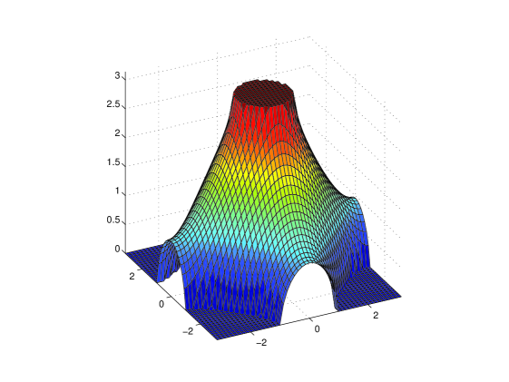
Figure 1: Level set of $e(p)=\alpha$ for $2<\alpha<4$

Let us briefly discuss the relation between the continuous and the lattice case in the random Schrödinger problem. The Four Denominator Estimate is used to control the recollision Feynman diagrams, as discussed in Section 1.2, for the discrete random Schrödinger evolution [7]. The same diagrams were estimated in the proof of the continuum model as well, [5]–[6]. The fundamental difference is that the level sets of the continuum dispersion relation, $e_{c}(p)=\frac{1}{2}p^{2}$, $p\in{\mathbb{R}}^{3}$, are uniformly convex surfaces (spheres). The level sets $\Sigma_{\alpha}=\{p\;:\;\alpha=e(p)\}\subset{\bf T}^{3}$ of the discrete dispersion relation (2.22) are uniformly convex only for $\alpha\in(0,2)\cup(4,6)$. For $\alpha\in(2,4)$, the level surfaces $\Sigma_{\alpha}$ are not convex, their Gauss curvature vanishes along a one-dimensional submanifold and they even contain straight lines (see Figure 1).

In the continuum model, the uniform convexity implies that a level set $\{p\;:\;\alpha=e_{c}(p)\}$ and its shifted copy $\{p\;:\;\alpha=e_{c}(p+q)\}$ have transversal intersection or they touch each other only at a point. This geometric fact is the key behind the Two Denominator Estimate for the continuous dispersion relation $e_{c}(p)=\frac{1}{2}p^{2}$ (see Lemma A.1 in [5]):

$$\sup_{\alpha}\int_{{\mathbb{R}}^{3}}\frac{{\rm d}\mu(p)}{|\alpha-e_{c}(p)+i\eta|\,|\alpha-e_{c}(p+q)+i\eta|}\leq\frac{C|\log\eta|^{2}}{|\!|\!|q|\!|\!|_{\eta}}$$ (2.27)

with $|\!|\!|q|\!|\!|_{\eta}=\eta+\min\{|q|,1\}$ and ${\rm d}\mu$ compactly supported. In particular, this estimate gives a short proof of the continuous version of the four-denominator estimate with a bound $C|\log\eta|^{4}$, since it allows one to eliminate two denominators by integrating out one free variable. The other two denominators can then be easily integrated out using (2.26).

A similar short proof of the four-denominator bound in the lattice case is not possible since the analogue of (2.27) does not hold for $\alpha\in(2,4)$. It is easy to see that the two-denominator integral ( (2.27) with $e(p)$ instead of $e_{c}(p)$) may be of order $\eta^{-1/2}$ if $q$ shifts along one of the straight line segments contained in $\Sigma_{\alpha}$. Actually, only a weaker upper bound of order $\eta^{-3/4}$ was proven in [7]. (T. Chen also proved in [3] a somewhat weaker three-denominator bound of order $\eta^{-4/5}$.) This bound is not sufficient to conclude the estimate of the recollision term for the lattice model in the same way as it was done for the continuous case in [5]–[6].

3 Proof of Theorem 2.1

In this section we fix $a\in{\cal I}$ and we will work on the surface $\Sigma_{a}$. We will define various quantities that depend on $a$. We will usually omit the dependence on $a$ in the notation, i.e. we write $\Sigma$, $\Gamma$, $p^{(j)}$, $N$, $d(p)$, $D(\zeta)$ etc. instead of $\Sigma_{a}$, $\Gamma_{a}$, $p^{(j)}_{a}$, $N_{a}$, $d_{a}(p)$, $D_{a}(\zeta)$, but all estimates and constants will be uniform in $a\in{\cal I}$. Let $\Omega=\{C_{0},C_{1},\ldots,C_{6}\}$ be the set of constants from (2.2) and Assumptions 1–4. Large or small positive constants depending on $\Omega$ will be denoted by $C_{\Omega}\gg 1$ or $0<c_{\Omega}\ll 1$ whose values may change from line to line. The notation $A\sim_{\Omega}B$ will refer to comparability up to $\Omega$-dependent positive constants, $c_{\Omega}\leq A/B\leq C_{\Omega}$. The notation $\sim$ will be used for comparability up to a universal constant.

3.1 Geometry at small Gauss curvature

We recall that the zero set $\Gamma={\cal G}\cap\Sigma$ is a finite union of disjoint regular curves. By (2.4) there exists a small constant $c_{0}$, depending on $C_{1},C_{2},C_{3}$, such that for each $a\in{\cal I}$ and all $|\varrho|\leq c_{0}$ the sets

$$\Gamma(\varrho)=\Sigma\cap{\cal G}(\varrho),\qquad{\cal G}(\varrho)=\{p\in{\cal D}:K(p)=\rho\}$$

are regular curves and they form a foliation in the tubular neighborhood

$${\cal N}=\{p\in\Sigma\;:\;|K(p)|<c_{0}\}$$ (3.1)

of the curves $\Gamma$ on the surface $\Sigma$. Moreover, by (2.5) we can choose $c_{0}$ so small that on each connected component of ${\cal N}$ one of the curvatures is much smaller than the other one. Then the principal curvatures and the principal curvature directions depend smoothly on $p\in{\cal N}$ with uniform bounds on the derivatives. We will work on one of these components that we continue to denote by ${\cal N}$, and for definiteness we assume $\kappa_{1}\ll\kappa_{2}$.

The principal curvature direction of $\kappa_{1}$ defines a smooth unit vectorfield in ${\cal N}$ that coincides with the vectorfield $Z$ on $\Gamma$ and hence it will also be denoted by $Z$.

Recall that by Assumption 4, there is a tangency of the integral curves of $Z$ and $W$ only at finitely many points, at most $N$ of them. We will present the proofs for the case $N\geq 1$. The case $N=0$ is much easier since these two foliations are uniformly transversal. We will not discuss this case in detail, but the statements made below remain valid.

Since $Z$ changes linearly in the neighborhood of the tangential points (Assumption 4) and $Z$ is regular, the points $\{p^{(j)}_{a}\;:j=1,\ldots,N_{a}\}$ are separated from each other, i.e.

$$c_{1}=\min_{a\in{\cal I}}\min_{j\neq k}|p^{(j)}_{a}-p^{(k)}_{a}|>0$$ (3.2)

and $c_{1}$ is bounded from below by a positive, $\Omega$-dependent constant. The uniformity in $a$ follows from the fact that the angle between $Z(p)$ and $w(p)$ is a regular function as $p$ moves on $\Gamma=\Gamma_{a}$, in particular its second derivative is bounded. Since near to a tangential point $p^{(j)}=p^{(j)}_{a}$ this angle increases linearly at a positive speed at least $C_{6}>0$ (uniformly in $a$), it cannot turn back to zero before $p$ moved at least a positive distance away from $p^{(j)}_{a}$. This shows the lower bound (3.2).

Figure 2: Foliations $\Gamma$ and $\gamma$ with their first order tangencies

The curves $\Gamma(\varrho)$, $|\varrho|\leq c_{0}$, form a regular foliation of ${\cal N}$ and $\Gamma$ is embedded in this foliation. The unit tangent vector to this foliation is $w(p)$ defined in (2.6). For any point $p\in{\cal N}$, let $\gamma_{p}\subset{\cal N}$ be the integral curve of $Z$ that goes through $p$. If $p^{(j)}$ is one of the points on $\Gamma$ from Assumption 4, then $\gamma_{j}=\gamma_{p^{(j)}}$ is tangent to $\Gamma$ at $p^{(j)}$, but their curvatures differ by the linear lower bound (2.9), i.e. the tangency of these two curves is precisely of first order (see Fig. 2).

The following lemma gives a lower bound on the transversality of the foliations $\gamma$ and $\Gamma$:

Lemma 3.1

For a sufficiently small $c_{0}$, depending only on $\Omega$, we have

$$p\in{\cal N}\;\;\Longrightarrow\;|Z(p)\times w(p)|\geq c_{\Omega}\cdot d(p)-C_{\Omega}|K(p)|\;.$$ (3.3)

Proof. If $N=0$, then (3.3) follows directly from (2.9) by regularity and $d(p)=1$ assuming $c_{0}$ is sufficiently small. Thus we can assume $N\geq 1$. Due to the regularity of the foliations $\gamma$ and $\Gamma=\{\Gamma(\varrho)\;:\;|\varrho|\leq c_{0}\}$ and due to their different curvatures at the tangential points, these two foliations can be mapped by a regular bijection $\Phi$ from the neighborhood of each tangential point in $\Sigma$ into the foliations $\{v=$ const $\}$ and $\{v=u^{2}\}$ in the $(u,v)\in{\mathbb{R}}^{2}$ plane near the origin.

Translating this picture into the $\gamma$ and $\Gamma$ foliations on $\Sigma$, this means that, for small enough $c_{0}$, there exist tangential points $p^{(j,\varrho)}\in\Gamma(\varrho)$, where the curves $\gamma_{j,\varrho}=\gamma_{p^{(j,\varrho)}}$ and $\Gamma(\varrho)$ have first order tangencies for any $|\varrho|\leq c_{0}$. For any $p\in{\cal N}$, we let

$$d^{(\varrho)}(p)=\min\{|p-p^{(j,\varrho)}|\;:\;1\leq j\leq N\},$$

where $\varrho$ is uniquely defined by $\varrho=K(p)$. Moreover, by the regularity of $\Phi$, the tangential points $p^{(j,\varrho)}$ are $C^{1}$ functions of $\varrho$ with bounded derivatives. In particular,

$$\big{|}d^{(\varrho)}(p)-d(p)\big{|}\leq C_{\Omega}|\varrho|,\quad\varrho=K(p),$$ (3.4)

uniformly in $p\in{\cal N}$, $a\in{\cal I}$, if $c_{0}$ is sufficiently small.

The regular bijection $\Phi$ also guarantees that the foliations $\gamma$ and $\Gamma$ have first order tangencies near the tangential points $p^{(j,\varrho)}$ on each $\Gamma(\varrho)$. For a sufficiently small $\Omega$-dependent positive constant $c_{2}\leq\frac{1}{2}c_{1}$ and by possibly reducing $c_{0}$ we thus have

$$|p-p^{(j,\varrho)}|\leq c_{2}\;\;\;\;\Longrightarrow\;\;\quad|Z(p)\times w(p)|\geq c_{\Omega}|p-p^{(j,\varrho)}|$$ (3.5)

for any $p\in{\cal N}$, $a\in{\cal I}$, $1\leq j\leq N$, where $\varrho=K(p)$.

Away from the tangential points, we first use

$$p\in\Gamma\;,\;d(p)\geq\frac{1}{2}\;c_{2}\;\;\Longrightarrow\;|Z(p)\times w(p)|\geq c_{\Omega}$$

by compactness and the continuity of the function $|Z(p)\times w(p)|$ on $\Gamma$ with zeros $p^{(j)}$. Then we extend this lower bound for $|\varrho|\leq c_{0}$ by continuity if $c_{0}$ is sufficiently small:

$$p\in\Gamma(\varrho)\;,\;d_{a,\varrho}(p)\geq c_{2}\;\;\Longrightarrow\;|Z(p)\times w(p)|\geq c_{\Omega}\;.$$ (3.6)

By combining this uniform bound with the estimate (3.5) near the tangential points and by using (3.4), we have

$$p\in\Gamma(\varrho),\;\;\Longrightarrow\;|Z(p)\times w(p)|\geq c_{\Omega}\cdot d^{(\varrho)}(p)\quad\mbox{with}\;\;\varrho=K(p)$$ (3.7)

By using (3.4), we obtain (3.3). $\;\;\Box$

In the stationary phase analysis we will have to estimate the volume of a regime $\{q\in\Sigma\;:\;K(q)\sim\varepsilon\}$ intersected with the preimage of a small spherical cap $C_{\delta}(\zeta)=\{{\omega}\in S^{2}\;:\;|{\omega}\times\zeta|\leq\delta\}$ around $\zeta\in S^{2}$ under the Gauss map $\nu:\Sigma\to S^{2}$. We thus define the set

$$C_{\varepsilon,\delta}(\zeta)=\Big{\{}q\in{\cal N}\;:\;\varepsilon\leq|K(q)|\leq 4\varepsilon\;,\;|\nu(q)\times\zeta|\leq\delta\Big{\}}\;.$$

for any $\zeta\in S^{2}$ (see Fig. 3).

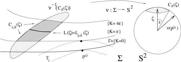
Figure 3: Intersection of $\varepsilon\leq K\leq 4\varepsilon$ and the preimage of the spherical cap $C_{\delta}(\zeta)$

Lemma 3.2

Let $c_{0}$ be sufficiently small, depending on $\Omega$, let $0<\varepsilon\leq c_{0}$ and $\delta>0$. Then for any $\zeta\in S^{2}$ at least one of the following holds:

$$\mbox{either}\quad\mbox{\rm vol}_{\Sigma}\;\big{[}C_{\varepsilon,\delta}(\zeta)\big{]}\leq\frac{C_{\Omega}\varepsilon\delta}{\big{[}D(\zeta)\big{]}^{1/2}}\;,\quad\mbox{or}\;\;D(\zeta)\leq C_{\Omega}(\varepsilon+\delta)\;.$$ (3.8)

Proof. We will work in one component of ${\cal N}$ and we recall that $\kappa_{1}\ll\kappa_{2}$ in this component, i.e. $\kappa_{2}\geq c_{\Omega}$ by (2.5) and $|\kappa_{1}|\sim_{\Omega}|K|$.

The principal curvature direction corresponding to $\kappa_{2}$ is orthogonal to the foliation $\gamma$, thus the normal vector $\nu(b)$ changes linearly with a coefficient proportional to $\kappa_{2}$ if the base point $b$ is moving transversally to $\gamma$. If $b$ moves along a curve $\gamma$, then the change is proportional to $\kappa_{1}$ (plus a quadratic correction):

$$|\nu(b)-\nu(b^{\prime})|\leq C_{\Omega}\Big{[}\;|b-b^{\prime}|^{2}+\big{(}\sup_{[b,b^{\prime}]}|\kappa_{1}|]\big{)}\;|b-b^{\prime}|\;\Big{]}$$ (3.9)

if $b^{\prime}\in\gamma_{b}$ and the supremum is taken on the curve segment between $b$ and $b^{\prime}$.

Let $q\in C_{\varepsilon,\delta}(\zeta)$ and let $d(q)=|q-p^{(j)}|$ for an appropriate $j$. Then the base point $q$ can first be moved transversally with a distance less than $C_{\Omega}|K(q)|$ to reach the curve $\gamma_{j}$, then it can be moved along this curve with a distance less than $C_{\Omega}d(q)$ to reach $p^{(j)}$. The motion stays in a neighborhood of $\Gamma$ of width comparable with $d(q)$ or smaller, so the Gauss curvature, and thus $\kappa_{1}$, is bounded by $C_{\Omega}d(q)$ along the whole motion.

From (3.9) we have

$$|\nu(q)\times\nu(p_{j})|\leq|\nu(q)-\nu(p_{j})|\leq C_{\Omega}(|K(q)|+d(q)^{2})$$ (3.10)

by using $|\nu\times\nu^{\prime}|\leq|\nu-\nu^{\prime}|$ for unit vectors. Furthermore, $q\in C_{\varepsilon,\delta}(\zeta)$ implies that $|\zeta\times\nu(q)|\leq\delta$, thus we obtain

$$D(\zeta)\leq C_{\Omega}(|K(q)|+d(q)^{2}+\delta)$$ (3.11)

since $|\nu\times\nu^{\prime\prime}|\leq(|\nu\times\nu^{\prime}|+|\nu^{\prime}-\nu^{\prime\prime}|)$ for unit vectors.

If there exists a point $q\in C_{\varepsilon,\delta}(\zeta)$ with $d(q)\leq C_{\Omega}|K(q)|^{1/2}$, then (3.11) implies the second statement of (3.8). For the rest of the proof we thus can assume that

$$\forall\;q\in C_{\varepsilon,\delta}(\zeta)\;\;\Longrightarrow\;\;C_{\Omega}|K(q)|^{1/2}\leq d(q)\;.$$ (3.12)

In particular, by (3.11),

$$D(\zeta)\leq C_{\Omega}(d(q)^{2}+\delta)\;,\qquad\forall\;q\in C_{\varepsilon,\delta}(\zeta)\;.$$ (3.13)

In this case we will show that $\mbox{vol}\big{[}C_{\varepsilon,\delta}(\zeta)\big{]}\leq C_{\Omega}\varepsilon\delta/[D(\zeta)]^{1/2}$. For $\varepsilon\leq|\varrho|\leq 4\varepsilon$, we define (see Fig. 3)

$$L(\zeta)=L_{\varrho,\delta}(\zeta)=\Gamma(\varrho)\cap C_{\varepsilon,\delta}(\zeta)=\Big{\{}q\in\Gamma(\varrho)\;:\;|\nu(q)\times\zeta|\leq\delta\Big{\}}\;.$$

Proposition 3.3

Suppose that (3.12) holds. Then the one-dimensional measure of $L(\zeta)$, as a subset of the curve $\Gamma(\varrho)$, satisfies

$$|L(\zeta)|\leq\frac{C_{\Omega}\delta}{\big{[}D(\zeta)\big{]}^{1/2}}$$ (3.14)

for any $\varepsilon\leq|\varrho|\leq 4\varepsilon$.

By this Proposition, the first statement in (3.8) follows by integration over $\varrho\in[\varepsilon,4\varepsilon]$ and by the regularity of the foliation $\Gamma$. This completes the proof of Lemma 3.2. $\;\;\Box$.

Proof of Proposition 3.3. We can assume that $\delta$ is small, otherwise (3.14) follows from the boundedness of $|\Gamma(\varrho)|$ and $D(\zeta)$. We now fix $\varrho\in\pm[\varepsilon,4\varepsilon]$ and define the set

$$W=W_{\varrho}=\Big{\{}q\in\Gamma(\varrho)\;:\;d(q)^{2}\geq c^{*}\Big{\}}\;,$$

where $c^{*}<1$ is a sufficiently small $\Omega$-dependent constant. By (3.2) and for a sufficiently small $c_{0}$ and $c^{*}$ it is clear that its complement $W^{c}=\Gamma(\varrho)\setminus W$ consists of at most $N$ connected pieces of $\Gamma(\varrho)$ and thus $W$ consists of at most $N+1$ pieces (in particular, if $N=0$, then $\Gamma(\varrho)=W$). Furthermore, we also define

$$U=U_{\varrho,\delta}=\Big{\{}q\in\Gamma(\varrho)\;:\;d(q)^{2}\leq\min\{\delta,c^{*}\}\Big{\}}\subset W^{c}\;,$$

that also consists of at most $N$ connected pieces. The complement

$$V=W^{c}\setminus U=\Big{\{}q\in\Gamma(\varrho)\;:\;\min\{\delta,c^{*}\}\leq d(q)^{2}\leq c^{*}\Big{\}}$$

thus consists of at most $2N$ connected pieces. The interesting case is when $\delta<c^{*}$, i.e. $V\neq\emptyset$ (see Fig. 4).

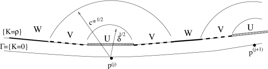
Figure 4: The subsets $U,V,W$ on the line $\Gamma_{\varrho}=\{K=\varrho\}$

We decompose

$$L(\zeta)=\big{(}L(\zeta)\cap U\big{)}\cup\big{(}L(\zeta)\cap V\big{)}\cup\big{(}L(\zeta)\cap W\big{)}$$

and estimate the length of each piece separately.

For the first piece, we use the trivial bound

$$|L(\zeta)\cap U|\leq|U|\leq C_{\Omega}N\delta^{1/2}\leq C_{\Omega}\delta^{1/2}\;,$$

as $U$ consists of at most $N$ pieces of length at most $\sim\delta^{1/2}$ and $N\leq C_{\Omega}$. The resulting $C_{\Omega}\delta^{1/2}$ can be bounded by $C_{\Omega}\delta/D(\zeta)^{1/2}$ since $D(\zeta)\leq C_{\Omega}\delta$ from (3.13) if $L(\zeta)\cap U\neq\emptyset$.

For the other two pieces, we recall the bound $|Z(q)\times w(q)|\geq c_{\Omega}\cdot d(q)-C_{\Omega}|K(q)|$ from (3.3). By the condition (3.12), $C_{\Omega}|K(q)|^{1/2}\leq d(q)$ holds on $L(\zeta)\subset C_{\varepsilon,\delta}(\zeta)$, so $|Z(q)\times w(q)|\geq c_{\Omega}\cdot d(q)$ if $c_{0}$ (hence $|K(q)|$) is sufficiently small. Thus the transversality angle between the two foliations is at least $c_{\Omega}d(q)$, i.e. $\nu(q)$ changes at least at a rate $\sim_{\Omega}d(q)$ as $q$ is moving along $L(\zeta)$

$$q\in L(\zeta)\;\;\;\Longrightarrow\;\;|\nabla_{w}\nu(q)|\geq c_{\Omega}d(q).$$ (3.15)

We need the following elementary lemma:

Lemma 3.4

i) Let $I$ be a compact interval and $g:I\to{\mathbb{R}}^{3}$ be a twice differentiable function with $\inf_{I}|g^{\prime}|\geq\lambda>0$. Then for any $\delta$ we have

$$\Big{|}\Big{\{}q\in I\;:\;|g(q)|\leq\delta\Big{\}}\Big{|}\leq 8\delta\lambda^{-1}+16|I|\delta\lambda^{-2}\max_{I}|g^{\prime\prime}|\;,$$ (3.16)

where $\big{|}\cdot\big{|}$ denotes the one-dimensional Lebesgue measure.

ii) Let $h:I\to{\mathbb{R}}$ with $\inf_{I}|h^{\prime}|\geq\lambda>0$ and assume that $h^{\prime}$ has a definite sign in $I$. Then

$$\Big{|}\Big{\{}q\in I\;:\;|h(q)|\leq\delta\Big{\}}\Big{|}\leq 4\delta\lambda^{-1}\;.$$ (3.17)

We will apply the first part of this lemma to the function $g(q)=\nu(q)\times\zeta$ along $\Gamma(\varrho)$ on each connected piece of $L(\zeta)\cap W$. Clearly $|g^{\prime\prime}|\leq C_{\Omega}$. Since $\nu$ is a normal vector, its variation along $\Gamma(\varrho)$, $\nabla_{w}\nu$, is orthogonal to $\nu$. Since $\nu$ and $\zeta$ are almost parallel on $L_{a,\varrho}(\zeta)$ (assuming $\delta\ll 1$), the variation of $g$ is comparable with the variation of $\nu$, i.e. $|\nabla_{w}g|\geq\frac{1}{2}|\nabla_{w}\nu|$. On $L(\zeta)\cap W$ we have $d(q)^{2}\geq c^{*}$, thus $|\nabla_{w}g|\geq c_{\Omega}$ from (3.15). By (3.16), we have

$$|L(\zeta)\cap W|\leq C_{\Omega}N\delta\leq C_{\Omega}\delta\;,$$

which is smaller than the bound (3.14) since $D(\zeta)\leq C_{\Omega}$.

Finally, we consider each connected piece of $L(\zeta)\cap V$. Let $S$ be one of them. Let $R(q)\in T_{p}\Sigma$ be the unit vectorfield orthogonal to $Z(q)$, i.e. it is the direction of principal curvature belonging to $\kappa_{2}$ (recall that $|\kappa_{2}|\geq c_{\Omega}$ on ${\cal N}$). We decompose the variation of $\nu$ along $\Gamma(\varrho)$ as

$$\nabla_{w}\nu=(\nabla_{w}\nu\cdot R)R+(\nabla_{w}\nu\cdot Z)Z=\kappa_{2}(R\cdot w)R+\kappa_{1}(Z\cdot w)Z\;,$$ (3.18)

by using $\nabla_{R}\nu\cdot R=\kappa_{2}$, $\nabla_{Z}\nu\cdot Z=\kappa_{1}$ and $\nabla_{R}\nu\cdot Z=\nabla_{Z}\nu\cdot R=0$.

Within $L(\zeta)$, the $R$-component of $\nabla_{w}\nu$ is bounded from below $|\nabla_{w}\nu(q)\cdot R(q)|\ =|\kappa_{2}||R(q)\cdot w(q)|\geq c_{\Omega}d(q)$ by (3.7). Moreover $\nabla_{w}\nu\cdot R=\kappa_{2}(R\cdot w)$ has a definite sign on $S$. The $Z$ component of $\nabla_{w}\nu$ is bounded by

$$|\nabla_{w}\nu(q)\cdot Z(q)|\leq C_{\Omega}|K(q)|\leq C_{\Omega}d(q)^{2}$$ (3.19)

by using $|\kappa_{1}|\leq C_{\Omega}|K|$ and (3.12).

Fix a point $q_{0}\in S$ and define $h(q)=R(q_{0})\cdot(\nu(q)-\zeta)$. Its derivative along $w$ is given by

$$h^{\prime}(q)=(\nabla_{w}\nu(q)\cdot R(q))(R(q)\cdot R(q_{0}))+(\nabla_{w}\nu(q)\cdot Z(q))(Z(q)\cdot R(q_{0}))$$ (3.20)

by using (3.18). For a sufficiently small $c^{*}$, the vectorfield $R$ does not change much on $S$, thus $R(q)\cdot R(q_{0})\geq\frac{1}{2}$ for all $q\in S$. Thus the first term in (3.20) has a definite sign and it is bigger than $c_{\Omega}d(q)$ in absolute value. The second term is smaller than $C_{\Omega}d(q)^{2}$. For a sufficiently small $c^{*}$ we thus have $|h^{\prime}(q)|\geq c_{\Omega}d(q)$ and $h^{\prime}$ has a definite sign. Moreover, on $V$, $d(q)^{2}\geq 2\delta$ implies $d(q)^{2}\geq c_{\Omega}D(\zeta)$, see (3.13). Thus for the function $h(q)$, defined on the connected piece $S$, it holds that $|h^{\prime}|\geq c_{\Omega}[D(\zeta)]^{1/2}$ and $h^{\prime}$ has definite sign.

Since $|\nu(q)\times\zeta|\geq c|\nu(q)-\zeta|\geq cR(q_{0})\cdot(\nu(q)-\zeta)=ch(q)$, we can directly apply (3.17) for each connected piece $S$ to obtain

$$|L(\zeta)\cap V|\leq\frac{C_{\Omega}N\delta}{\big{[}D(\zeta)\big{]}^{1/2}}\;,$$

and the proof of Proposition 3.3 is complete. $\;\;\Box$

Proof of Lemma 3.4. We denote $M=\max_{I}|g^{\prime\prime}|$. Let $q_{0}\in I$ be a point with $|g(q_{0})|\leq\delta$. By Taylor expansion,

$$|g(q)|\geq|g^{\prime}(q_{0})||q-q_{0}|-|g(q_{0})|-M|q-q_{0}|^{2}\;.$$

i.e. $|g(q)|>\delta$ if $\frac{4\delta}{\lambda}<|q-q_{0}|\leq\frac{\lambda}{2M}$. Thus within the interval $q\in[q_{0}-\frac{\lambda}{2M},q_{0}+\frac{\lambda}{2M}]\cap I$ only a subset of measure at most $\frac{8\delta}{\lambda}$ can satisfy $|g(q)|\leq\delta$, i.e. the density of the set $\{|g|\leq\delta\}$ is not bigger than $\max\{16\delta M\lambda^{-2},8\delta/(\lambda|I|)\}$. This proves (3.16). The proof of (3.17) is similar, by noticing that $|h(q)|>\delta$ if $2\delta/\lambda\leq|q-q_{0}|$. $\;\;\Box$

3.2 Dyadic decomposition

For any vector $\xi\in{\mathbb{R}}^{3}$, let $\xi=r{\omega}_{\xi}$ be its polar decomposition with $r=|\xi|$, ${\omega}_{\xi}\in S^{2}$. We will estimate $\widehat{\mu}_{a}(\xi)$ and we will omit $a$ from the notation as before.

We recall the definition of ${\cal N}$ from (3.1) and we assume that $c_{0}$ is so small as required in Lemma 3.1 and 3.2. Let $S_{0}=\Sigma\setminus{\cal N}$ be the complement of this neighborhood. Let $1\leq k\leq L$ be an integer and set

$$S_{k}=\{p\in\Sigma\;:\;2^{-k}c_{0}\leq|K(p)|\leq 2^{-k+2}c_{0}\}\;.$$ (3.21)

We also set

$$S_{\infty}=\{p\in\Sigma\;:\;|K(p)|\leq 2^{-L+1}c_{0}\}\;,$$

then $S_{0},S_{1},\ldots,S_{\infty}$ cover $\Sigma$ with overlaps. For the two-dimensional (surface) volume of these sets, we clearly have

$$\mbox{vol}(S_{k})\sim_{\Omega}2^{-k},\quad k\leq L,\quad\mbox{and}\quad\mbox{vol}(S_{\infty})\leq C_{\Omega}\cdot 2^{-L}\;.$$

We will say that two domains are regular bijective images of each other if there is a diffeomorphism $\Phi$ between them such that the derivatives of $\Phi$ and $\Phi^{-1}$ are both bounded with a $\Omega$-dependent uniform constant.

Since each $S_{k}$, $k\geq 1$, is the difference of level sets of the regularly foliating function $K(p)$, it is a regular bijective image of finitely many elongated rectangles with side-lengths $2^{-k}\times 1$. Similarly, $S_{0}$ can be written as a complement of regular images of finitely many rectangles. Therefore there exists a partition of unity, $\psi_{0},\psi_{1},\ldots,\psi_{L},\psi_{\infty}$, such that $\sum_{k=0}^{L}\psi_{k}+\psi_{\infty}\equiv 1$, $0\leq\psi_{k}\leq 1$, and

$$\mbox{supp}\;\psi_{\infty}\subset S_{\infty},\quad\mbox{supp}\;\psi_{k}\subset S_{k}\qquad|\partial^{\alpha}\psi_{k}|\leq C_{\Omega,\alpha}2^{|\alpha|k},\quad 0\leq k\leq L$$ (3.22)

for any multiindex $\alpha$ and $\psi_{\infty}$ satisfies the same bounds as $\psi_{L}$. The constants $C_{\Omega,\alpha}$ depend on the $\alpha$ and $\Omega$.

We split the integral defining $\widehat{\mu}$ as follows

$$\widehat{\mu}(\xi)=I_{\infty}(\xi)+I_{0}(\xi)+\sum_{k=1}^{L}I_{k}(\xi)$$ (3.23)

with

$$I_{k}(\xi)=\int_{\Sigma}e^{i\xi\cdot p}\;\psi_{k}(p)f(p){\rm d}m(p)\;.$$

By the estimate on $\mbox{vol}(S_{\infty})$, we obtain

$$\sup_{\xi\in{\mathbb{R}}^{3}}|I_{\infty}(\xi)|\leq C^{*}\cdot 2^{-L}\;$$ (3.24)

(recall that $C^{*}$ denotes a constant depending on $\Omega$ and $f$).

To estimate $\sum_{k=1}^{L}I_{k}(\xi)$, we define

$$R_{j}=\{{\omega}\in S^{2}\;:\;2^{-j}\leq|{\omega}\times{\omega}_{\xi}|\leq 2^{-j+2}\}$$ (3.25)

for $j=0,1,2,\ldots$. Notice that $R_{j}$ consists of two antipodal spherical annuli with inner radius and width comparable with $2^{-j}$ and $R_{j}$ lies in two antipodal spherical caps: $R_{j}\subset C_{j}^{+}\cup C_{j}^{-}$ with

$$C_{j}^{\pm}=\{{\omega}\in S^{2}\;:\;2^{-j-1}\leq|{\omega}\mp{\omega}_{\xi}|\leq 2^{-j+3}\}\;.$$

We define a partition of unity $0\leq\varphi_{j}\leq 1$ on $S^{2}\setminus\{\pm{\omega}_{\xi}\}$ such that

$$\sum_{j=0}^{\infty}\varphi_{j}\equiv 1,\qquad\mbox{supp}\;\varphi_{j}\subset R_{j},\qquad|\partial^{\alpha}\varphi_{j}|\leq C_{\alpha}\cdot 2^{|\alpha|j}$$ (3.26)

for any multiindex $\alpha$, and we write, for any $1\leq k\leq L$,

$$I_{k}(\xi)=\sum_{j=0}^{\infty}I_{k,j}(\xi),\qquad I_{k,j}(\xi)=\int_{\Sigma}e^{ip\cdot\xi}\;\psi_{k}(p)\varphi_{j}(\nu(p))f(p){\rm d}m(p)\;.$$ (3.27)

Let

$$U_{k,j}=S_{k}\cap\nu^{-1}(R_{j})\;,$$

where $\nu:\Sigma\to S^{2}$ is the normal map (2.7). Then the integration domain for $I_{k,j}$ is contained in $U_{k,j}$,

$$\mbox{supp}(\psi_{k})\cap\mbox{supp}(\varphi_{j}\circ\nu)\subset U_{k,j}\;.$$

By a trivial supremum bound we have

$$|I_{k,j}(\xi)|\leq C^{*}\cdot\mbox{vol}(U_{k,j})\;,$$ (3.28)

in particular

$$|I_{k,j}(\xi)|\leq C^{*}\;.$$ (3.29)

3.3 A stationary phase lemma

We need the following Lemma:

Lemma 3.5

Let $Q$ be a smooth function supported in a sufficiently small subset $U\subset\Sigma$ so that $|\partial e(p)/\partial p_{3}|\geq c_{\Omega}$ holds for $p\in U$. Suppose that on this neighborhood $|\nu(p)\times{\omega}_{\xi}|\geq\delta>0$. Then

$$\Bigg{|}\int_{\Sigma}e^{ip\cdot\xi}Q(p){\rm d}m(p)\Bigg{|}\leq\frac{C_{\Omega}}{|\xi|}\cdot\mbox{\rm vol}_{\Sigma}(U)\cdot\Big{(}\delta^{-2}\|Q\|_{\infty}+\delta^{-1}\|Q\|_{C^{1}}\Big{)}\;.$$ (3.30)

Proof of Lemma 3.5. On the subset $U$, the surface $\Sigma$ can be coordinatized by $p_{1},p_{2}$, i.e. $U$ embedded in ${\mathbb{R}}^{3}$ or ${\bf T}^{3}$ can be described as a regular function $p_{3}=p_{3}(p_{1},p_{2})$ with uniformly bounded derivatives. After a change of variables, we have (with ${\omega}_{\xi}=({\omega}_{\xi,1},{\omega}_{\xi,2},{\omega}_{\xi,3})$)

$$\int_{\Sigma}e^{ip\cdot\xi}Q(p){\rm d}m(p)=\int_{\pi(U)}e^{i|\xi|(p_{1}{\omega}_{\xi,1}+p_{2}{\omega}_{\xi,2}+p_{3}(p_{1},p_{2}){\omega}_{\xi,3})}\widetilde{Q}(p_{1},p_{2}){\rm d}p_{1}{\rm d}p_{2}$$ (3.31)

where $\widetilde{Q}(p_{1},p_{2})=Q(p)(1+|\nabla p_{3}|^{2})^{1/2}$ is evaluated at $p=(p_{1},p_{2},p_{3}(p_{1},p_{2}))$ and $\pi(U)$ is the projection of $U$ onto the $(p_{1},p_{2})$-plane. The Jacobian can be computed as

$$(1+|\nabla p_{3}|^{2})^{1/2}=|\nabla e|\,\Big{|}\frac{\partial e}{\partial p_{3}}\Big{|}^{-1}\;,$$

by differentiating the defining equation $e(p_{1},p_{2},p_{3}(p_{1},p_{2}))=a$,

$$\frac{\partial p_{3}}{\partial p_{1}}=-\frac{\nu_{1}(p)}{\nu_{3}(p)},\qquad\frac{\partial p_{3}}{\partial p_{2}}=-\frac{\nu_{2}(p)}{\nu_{3}(p)}\;,$$ (3.32)

and by using (2.7).

The gradient of the phase factor in (3.31), as a function of $(p_{1},p_{2})$, can be estimated from below by

$$\Big{|}\nabla_{(p_{1},p_{2})}(p_{1}{\omega}_{\xi,1}+p_{2}{\omega}_{\xi,2}+p_{3}(p_{1},p_{2}){\omega}_{\xi,3})\Big{|}\geq\frac{1}{\sqrt{2}}\Big{|}{\omega}_{\xi,1}+\frac{\partial p_{3}}{\partial p_{1}}{\omega}_{\xi,3}\Big{|}+\frac{1}{\sqrt{2}}\Big{|}{\omega}_{\xi,2}+\frac{\partial p_{3}}{\partial p_{2}}{\omega}_{\xi,3}\Big{|}\;.$$

For any two vectors, $\nu,{\omega}\in{\mathbb{R}}^{3}$, with $\nu_{3}\neq 0$ we have

$$|{\omega}\times\nu|\leq\Big{|}{\omega}_{1}-\frac{\nu_{1}}{\nu_{3}}{\omega}_{3}\Big{|}\,\big{(}|\nu_{2}|+|\nu_{3}|\big{)}+\Big{|}{\omega}_{2}-\frac{\nu_{2}}{\nu_{3}}{\omega}_{3}\Big{|}\,\big{(}|\nu_{1}|+|\nu_{3}|\big{)}\;,$$

i.e.

$$|{\omega}_{\xi}\times\nu(p)|\leq 2\Bigg{(}\Big{|}{\omega}_{\xi,1}-\frac{\nu_{1}(p)}{\nu_{3}(p)}{\omega}_{\xi,3}\Big{|}+\Big{|}{\omega}_{\xi,2}-\frac{\nu_{2}(p)}{\nu_{3}(p)}{\omega}_{\xi,3}\Big{|}\Bigg{)}\;,$$

since $\|\nu\|=1$. Therefore, by using (3.32), the gradient of the phase factor in (3.31) is bounded from below by $\frac{1}{\sqrt{8}}\,|{\omega}_{\xi}\times\nu(p)|\,|\xi|\geq\frac{1}{\sqrt{8}}\,\delta|\xi|$. The estimate (3.30) then follows by standard integration by parts by using (2.2), (2.3) and the lower bound on $|\partial e(p)/\partial p_{3}|$. $\;\;\Box$

3.4 The estimate of $I_{k,j}(\xi)$

Applying Lemma 3.5 to our integral $I_{k,j}(\xi)$, we obtain

$$|I_{k,j}(\xi)|\leq\frac{C_{\Omega}}{|\xi|}\cdot\mbox{vol}(U_{k,j})\Bigg{(}2^{2j}\cdot\|f\|_{\infty}+2^{j}\cdot\big{\|}\psi_{k}(p)\varphi_{j}(\nu(p))f(p)\big{\|}_{C^{1}}\Bigg{)}$$ (3.33)

by using that on the integration domain $|\nu(p)\times{\omega}_{\xi}|\geq 2^{-j}$ by (3.25).

From (2.2), (2.3) and from the bounds (3.22), (3.26) we have

$$\big{\|}\psi_{k}(p)\varphi_{j}(\nu(p))f(p)\big{\|}_{C^{1}}\leq C^{*}\max\{2^{k},2^{j}\}$$

i.e.

$$|I_{k,j}(\xi)|\leq\frac{C^{*}}{|\xi|}\cdot\mbox{vol}(U_{k,j})\cdot\max\{2^{k+j},2^{2j}\}\;.$$ (3.34)

Interpolating it with (3.28), we have

$$|I_{k,j}(\xi)|\leq\frac{C^{*}}{|\xi|^{3/4}}\cdot\Big{[}\max\{2^{k+j},2^{2j}\}\Big{]}^{3/4}\cdot\mbox{vol}(U_{k,j})\;.$$ (3.35)

The domain $U_{k,j}$ is contained in $\nu^{-1}(R_{j})$, so its volume is bounded by

$$\mbox{vol}(U_{k,j})\leq C_{\Omega}\cdot 2^{k}\cdot\mbox{vol}(R_{j})\leq C_{\Omega}\cdot 2^{k-2j},$$ (3.36)

using that the Jacobian of $\nu^{-1}$ is $|K|^{-1}\sim 2^{k}$ on the support of $\psi_{k}$ and the number of preimages is bounded by (2.8). We also have

$$\mbox{vol}(U_{k,j})\leq\mbox{vol}(S_{k})\leq C_{\Omega}\cdot 2^{-k}\;.$$ (3.37)

By (3.28) and (3.36), we have

$$\sum_{k=1}^{L}\sum_{j=L}^{\infty}|I_{k,j}(\xi)|\leq C^{*}\cdot 2^{-L}\;,$$ (3.38)

so these terms can be combined with the bound (3.24) and from now on we can assume that $j\leq L$.

To estimate $I_{k,j}(\xi)$ for $1\leq k\leq L$, $0\leq j\leq L$, we use Lemma 3.2 to estimate $\mbox{vol}(U_{k,j})$. Clearly $U_{k,j}\subset C_{\varepsilon,\delta}({\omega}_{\xi})$ with the choice $\varepsilon=2^{-k}c_{0}$, $\delta=2^{-j+2}$ and we obtain that either $\mbox{vol}(U_{k,j})\leq C_{\Omega}\cdot 2^{-k-j}D({\omega}_{\xi})^{-1/2}$ or $D({\omega}_{\xi})\leq C_{\Omega}(2^{-k}+2^{-j})$. In the first case, combining this estimate with (3.36) and (3.37), we obtain

$$\mbox{vol}(U_{k,j})\leq C_{\Omega}\cdot\min\Bigg{\{}2^{-k}\;,\;\frac{2^{-k-j}}{\big{[}D({\omega}_{\xi})\big{]}^{1/2}}\;,\;\frac{2^{-\frac{3}{2}j}}{\big{[}D({\omega}_{\xi})\big{]}^{1/4}}\Bigg{\}}\;,$$ (3.39)

so together with (3.35) and the boundedness of $D({\omega}_{\xi})$, we have

$$|I_{k,j}(\xi)|\leq\frac{C^{*}}{|\xi|^{3/4}\big{[}D({\omega}_{\xi})\big{]}^{1/2}}\;.$$ (3.40)

In the second case we use the trivial estimate (3.28)

$$|I_{k,j}(\xi)|\leq\mbox{vol}(U_{k,j}){\bf 1}\big{[}D({\omega}_{\xi})\leq C_{\Omega}(2^{-k}+2^{-j})\;\big{]}\;,$$

where ${\bf 1}[\ldots]$ is the characteristic function. We combine it with (3.34) and with the bound $\mbox{vol}(U_{k,j})\leq C_{\Omega}\cdot\min\{2^{-k},2^{k-2j}\}$ from (3.36), (3.37), to obtain

$$|I_{k,j}(\xi)|\leq\frac{C^{*}}{|\xi|^{3/4}}\cdot\Big{[}\max\{2^{k+j},2^{2j}\}\Big{]}^{3/4}\cdot\min\{2^{-k},2^{k-2j}\}\cdot{\bf 1}\big{[}D({\omega}_{\xi})\leq C_{\Omega}(2^{-k}+2^{-j})\;\big{]}\;.$$

It is easy to check by separating the $k\leq j$ and $k\geq j$ cases, that we obtain the same bound (3.40) as in the first case. Together with the trivial estimate (3.29), we thus have

$$|I_{k,j}(\xi)|\leq\frac{C^{*}}{\big{\langle}|\xi|^{3/4}\big{[}D({\omega}_{\xi})\big{]}^{1/2}\big{\rangle}}\;$$ (3.41)

in both cases.

Finally, we estimate $I_{0}(\xi)$. For sufficiently small $c_{0}$, the boundaries of $S_{0}$ and $S_{1}$ consist of regular curves. We can find finitely many open balls that cover $S_{0}$ and lie within $S_{1}\cup S_{0}$. The number of the balls is bounded by a $\Omega$-dependent number by compactness for $a\in{\cal I}$. With an appropriate partition of unity, the integral $I_{0}(\xi)$ is decomposed into a finite sum of integrals of the form

$$\int_{D}e^{ip\cdot\xi}\;\psi_{D}(p)f(p){\rm d}m(p)$$

where $D\subset S_{1}\cup S_{0}$ is a disk of radius at least $c_{\Omega}$ and the smooth cutoff function is supported on $D$. Since the Gauss curvature of $\Sigma$ is uniformly bounded from below on $D$, by standard stationary phase estimate we obtain

$$|I_{0}(\xi)|\leq\frac{C^{*}}{\langle\xi\rangle}\;.$$ (3.42)

Collecting the estimates (3.38), (3.41) and (3.42) for the decompositions (3.23), (3.27), we have proved (2.13) in Theorem 2.1.

The proof of (2.14) is similar, we just sketch the key steps. We define the sets $S_{k}$ (3.21) for all $k\geq 1$ and the set $S_{\infty}$ will be absent. The partition of unity, $\psi_{0},\psi_{1},\ldots$ consists of infinitely many functions and $\sum_{k=0}^{\infty}\psi_{k}\equiv 1$ on the set $\Sigma\setminus\Gamma$ of full measure. Similarly, we extend the definition of $I_{k,j}$ (3.27) for any $k\geq 1$ and we use the decomposition

$$\widehat{\mu}(\xi)=I_{0}(\xi)+\sum_{k=1}^{\infty}\sum_{j=0}^{\infty}I_{k,j}(\xi)\;.$$

We now follow the previous argument. The interpolation (3.35) is modified to

$$|I_{k,j}(\xi)|\leq\frac{C^{*}}{|\xi|^{\frac{3}{4}-\beta}}\cdot\Big{[}\max\{2^{k+j},2^{2j}\}\Big{]}^{\frac{3}{4}-\beta}\cdot\mbox{vol}(U_{k,j})\;.$$ (3.43)

First, we consider the case when $\mbox{vol}(U_{k,j})\leq C_{\Omega}\cdot 2^{-k-j}D({\omega}_{\xi})^{-1/2}$, i.e. let

$$\Xi=\Big{\{}(k,j)\;:\;\mbox{vol}(U_{k,j})\leq C_{\Omega}\cdot 2^{-k-j}D({\omega}_{\xi})^{-1/2}\Big{\}}\subset{\bf N}_{+}\times{\bf N}$$

be the set of the corresponding indices. For $k\leq j$, $(k,j)\in\Xi$, we use the bound $2^{-\frac{3}{2}j}[D({\omega}_{\xi})]^{-1/4}$ for $\mbox{vol}(U_{k,j})$ from (3.39). The double summation over $k,j$ can be performed as

$$\sum_{(k,j)\in\Xi\;:\;k\leq j}|I_{k,j}(\xi)|\leq\frac{C^{*}}{|\xi|^{\frac{3}{4}-\beta}\big{[}D({\omega}_{\xi})\big{]}^{1/4}}\sum_{k=1}^{\infty}\sum_{j=k}^{\infty}2^{-2j\beta}\leq\frac{C^{*}\beta^{-2}}{|\xi|^{\frac{3}{4}-\beta}\big{[}D({\omega}_{\xi})\big{]}^{1/4}}\;.$$

For $k>j$, we use the bound $2^{-k-\frac{3}{4}j}[D({\omega}_{\xi})]^{-\frac{3}{8}}$ for $\mbox{vol}(U_{k,j})$ from the first two terms in (3.39) and thus

$$\sum_{(k,j)\in\Xi\;:\;k>j}|I_{k,j}(\xi)|\leq\frac{C^{*}}{|\xi|^{\frac{3}{4}-\beta}\big{[}D({\omega}_{\xi})\big{]}^{3/8}}\sum_{j=0}^{\infty}\sum_{k=j+1}^{\infty}2^{-\frac{1}{4}k}\leq\frac{C^{*}}{|\xi|^{\frac{3}{4}-\beta}\big{[}D({\omega}_{\xi})\big{]}^{3/8}}\;.$$

On the complement of $\Xi$, when $D({\omega}_{\xi})\leq C_{\Omega}(2^{-k}+2^{-j})$, we again distinguish whether $k\leq j$ or $k>j$. If $k\leq j$, then we use $\mbox{vol}(U_{k,j})\leq C_{\Omega}\cdot 2^{k-2j}$ from (3.36) to obtain

$$\sum_{(k,j)\not\in\Xi\;:\;k\leq j}|I_{k,j}(\xi)| \leq\frac{C^{*}}{|\xi|^{\frac{3}{4}-\beta}}\sum_{k=1}^{\infty}\sum_{j=k}^{\infty}2^{(\frac{1}{2}-\beta)k}\cdot 2^{-j\beta}\cdot{\bf 1}\big{[}(k,j)\not\in\Xi\big{]}$$

$$\leq\frac{C^{*}\beta^{-2}}{|\xi|^{\frac{3}{4}-\beta}\big{[}D({\omega}_{\xi})\big{]}^{\frac{1}{2}-\beta}}\;,$$

after replacing $2^{k}\leq[D({\omega}_{\xi})]^{-1}$ in the first factor and using the second one, $2^{-j\beta}$, to perform the double summation.

Finally, if $j<k$, we use $\mbox{vol}(U_{k,j})\leq C_{\Omega}\cdot 2^{-k}$ from (3.37), to obtain

$$\sum_{(k,j)\not\in\Xi\;:\;j<k}|I_{k,j}(\xi)| \leq\frac{C^{*}}{|\xi|^{\frac{3}{4}-\beta}}\sum_{j=0}^{\infty}\sum_{k=j+1}^{\infty}2^{(\frac{1}{2}-\beta)j}\cdot 2^{-k\beta}\cdot{\bf 1}\big{[}(k,j)\not\in\Xi\big{]}$$

$$\leq\frac{C^{*}\beta^{-2}}{|\xi|^{\frac{3}{4}-\beta}\big{[}D({\omega}_{\xi})\big{]}^{\frac{1}{2}-\beta}}\;.$$

Collecting these estimates together with (3.42) and the boundedness of $D$ and $|\widehat{\mu}|$, we obtain (2.14). $\;\;\;\Box$

3.5 Proof of Corollary 2.2

For the proof of (2.15), choose $L=\log_{2}M$ in (2.13), then with $\xi=r{\omega}$, $r\geq 0$, ${\omega}\in S^{2}$,

$$\int_{|\xi|\leq M}|\widehat{\mu}(\xi)|^{4}{\rm d}\xi\leq C^{*}+C^{*}L^{8}\int_{1}^{2^{L}}r^{2}{\rm d}r\int_{S^{2}}\frac{{\rm d}m({\omega})}{\big{\langle}r^{3}D({\omega})^{2}\rangle}\;,$$ (3.44)

where ${\rm d}m$ denotes the surface measure on $S^{2}$. Using $r\leq 2^{L}$ we can estimate the second integral:

$$\int_{S^{2}}\frac{{\rm d}m({\omega})}{\big{\langle}r^{3}D({\omega})^{2}\rangle} \leq\frac{1}{r^{3}}\int_{S^{2}}\frac{{\bf 1}\big{[}D({\omega})\geq 2^{-\frac{3}{2}L}\big{]}}{D({\omega})^{2}}\;{\rm d}m({\omega})+\int_{S^{2}}{\bf 1}\big{[}D({\omega})\leq 2^{-\frac{3}{2}L}\big{]}\;{\rm d}m({\omega})$$

$$\leq\frac{1}{r^{3}}\sum_{\pm}\sum_{j=1}^{N}\int_{S^{2}}\frac{{\bf 1}\big{[}|{\omega}\pm\nu(p^{(j)})|\geq 2^{-\frac{3}{2}L}\big{]}}{|{\omega}\pm\nu(p^{(j)})|^{2}}\;{\rm d}m({\omega})+CN\cdot 2^{-3L}$$

$$\leq\frac{CNL}{r^{3}}+CN\cdot 2^{-3L}$$

by the definition (2.12) of $D({\omega})$. Inserting this bound into (3.44), we obtain (2.15).

For the proof of (2.16) we first notice that by interpolation and $\|\widehat{\mu}\|_{\infty}\leq C^{*}$, it is sufficient to prove this bound for all small positive $\beta$. For a given $0<\beta<2/5$ we use (2.14) with $5\beta/32$ instead of $\beta$ to obtain

$$\int_{{\mathbb{R}}^{3}}|\widehat{\mu}(\xi)|^{4+\beta}{\rm d}\xi \leq C^{*}+C^{*}\beta^{-2(4+\beta)}\int_{{\mathbb{R}}^{3}}\frac{{\bf 1}\{|\xi|\geq 1\}\;{\rm d}\xi}{\big{\langle}|\xi|^{\frac{3}{4}-\frac{5}{32}\beta}|D({\omega}_{\xi})|^{\frac{1}{2}-\frac{5}{32}\beta}\big{\rangle}^{4+\beta}}$$

$$\leq C^{*}+C^{*}\beta^{-2(4+\beta)}\int_{{\mathbb{R}}^{3}}\frac{{\bf 1}\{|\xi|\geq 1\}\;{\rm d}\xi}{|\xi|^{3+\frac{1}{16}\beta}|D({\omega}_{\xi})|^{2-\frac{1}{8}\beta}+1}$$

$$\leq C^{*}+C^{*}\beta^{-2(4+\beta)}\int_{S^{2}}\frac{{\rm d}m({\omega})}{|D({\omega})|^{\frac{96-3\beta}{48+\beta}}}\int_{1}^{\infty}\frac{{\rm d}u}{u^{3+\frac{1}{16}\beta}+1}$$

$$\leq C^{*}\beta^{-10-2\beta}\;.\qquad\Box$$

4 Proof of the Four Denominator Estimate

We fix $\alpha$, $\eta$, $\Lambda$ and $u$ throughout the proof. $C_{\Lambda}$ and $c_{\Lambda}$ will denote large and small universal positive constants depending only on $\Lambda$. We will mostly omit the $\alpha$ and $u$-dependence in the notation, all estimates are uniform for $u\in{\mathbb{R}}^{3}$ and $\alpha\in{\mathbb{R}}$ with $|\!|\!|\alpha|\!|\!|\geq\Lambda$.

We recall the definition of $e(p)$ from (2.22). The range of $e(p)$ is $[0,6]$. Let $0\leq\chi(t)\leq 1$ be a smooth cutoff function on $[0,6]$ such that $\chi(t)\equiv 1$ if $|\!|\!|t|\!|\!|\geq 2\Lambda/3$ and $\chi(t)\equiv 0$ if $|\!|\!|t|\!|\!|\leq\Lambda/3$, $|\partial^{\alpha}\chi|\leq C_{\alpha}\Lambda^{-\alpha}$, where $|\!|\!|\cdot|\!|\!|$ is defined in (2.24).

We insert $1\equiv\chi(e(p))+[1-\chi(e(p))]$ in the integral $I_{\alpha,\eta}(u)$ (2.23). On the set where $1-\chi(e(p))\neq 0$ we can estimate

$$\frac{1}{|\alpha-e(p)+i\eta|}\leq C\Lambda^{-1}\;,$$

and once one of the denominators is eliminated, the rest can be integrated out at the expense of $C|\log\eta|^{3}$, see (2.26).

So we can focus on the term with $\chi(e(p))$. Similarly we can insert $\chi(e(q))\chi(e(r))\chi(e(p+q+r-u))$ as well and we define

$$I=\int\frac{\chi(e(p))\chi(e(q))\chi(e(r))\chi(e(p+q+r-u))dpdqdr}{|\alpha-e(p)+i\eta||\alpha-e(q)+i\eta||\alpha-e(r)+i\eta||\alpha-e(p-q+r-u)+i\eta|}\;.$$

Then

$$I_{\alpha,\eta}(u)\leq C_{\Lambda}|\log\eta|^{3}+I\;.$$ (4.1)

We set

$$I(\xi)=\int_{{\bf T}^{3}}\frac{e^{ip\cdot\xi}\chi(e(p))}{|\alpha-e(p)+i\eta|}\;{\rm d}p$$ (4.2)

for $\xi\in{\mathbb{R}}^{3}$, then clearly $I(\xi)=I(-\xi)$ and it is real. Moreover

$$I=\frac{1}{2\pi}\int_{{\mathbb{R}}^{3}}{\rm d}\xi\;I(\xi)^{4}\;e^{-iu\cdot\xi}\leq\int_{{\mathbb{R}}^{3}}{\rm d}\xi|I(\xi)|^{4}\;.$$

The function $h(p)=\chi(e(p))|\alpha-e(p)+i\eta|^{-1}$ in the oscillatory integral (4.2) is regular on scale $\eta$,

$$|\partial^{\beta}h(p)|\leq\frac{C_{\Lambda,\beta}\cdot\eta^{-|\beta|}}{|\alpha-e(p)+i\eta|}$$

for any multiindex $\beta$. Thus, by a standard stationary phase estimate and (2.26), we easily see that

$$|I(\xi)|\leq\frac{C_{\Lambda}|\log\eta|}{\langle\eta|\xi|\rangle}\;,$$

therefore

$$I\leq C_{\Lambda}|\log\eta|^{4}+\int_{|\xi|\leq\eta^{-4}}|I(\xi)|^{4}{\rm d}\xi\;.$$ (4.3)

By the coarea formula

$$I(\xi)=\int_{0}^{6}\frac{\chi(a){\rm d}a}{|\alpha-a+i\eta|}\;\widehat{\mu}_{a}(\xi)$$

with

$$\widehat{\mu}_{a}(\xi)=\int_{\Sigma_{a}}\frac{e^{ip\cdot\xi}}{|\nabla e(p)|}\;{\rm d}m_{a}(p)\;,$$

where we recall that ${\rm d}m_{a}$ is the uniform surface measure on the set $\Sigma_{a}=\{p\;:\;e(p)=a\}\subset{\bf T}^{3}$. Clearly $\widehat{\mu}_{a}(\xi)$ is an integral of the form (2.1) with $f(p)=|\nabla e(p)|^{-1}$. Note that

$$|\!|\!|a|\!|\!|^{1/2}\leq C\Big{(}\sum_{j=1}^{3}\sin^{2}p_{j}\Big{)}^{1/2}=C|\nabla e(p)|\;.$$ (4.4)

Thus for $|\!|\!|a|\!|\!|\geq\Lambda/3$, the function $|\nabla e(p)|$ on the set $\Sigma_{a}$ is separated away from zero and is smooth with derivatives bounded uniformly in $a$ (depending only on $\Lambda$), so $|\nabla e(p)|^{-1}$ is smooth.

The main technical result is the following special case of Corollary 2.2 for the family of level sets $\{e(p)=a\}$ with values in the compact set ${\cal I}=\{a\in[0,6]\;:\;|\!|\!|a|\!|\!|\geq\Lambda/3\}$.

Proposition 4.1

Let $0<\Lambda<1/2$. For any $a$ with $|\!|\!|a|\!|\!|\geq\Lambda$, we have

$$\int_{|\xi|\leq\eta^{-4}}|\widehat{\mu}_{a}(\xi)|^{4}{\rm d}\xi\leq C_{\Lambda}|\log\eta|^{10}\;.$$

The proof amounts to checking the assumptions in Corollary 2.2. Assumption 1 (formula (2.3)) has been checked in (4.4). The other three assumptions will be proven starting from the next section.

From this Proposition and (4.1), (4.3), the Four Denominator Estimate (2.25) easily follows. By Jensen’s inequality,

$$\int_{|\xi|\leq\eta^{-4}}{\rm d}\xi|I(\xi)|^{4} =\int_{|\xi|\leq\eta^{-4}}{\rm d}\xi\Bigg{|}\int_{0}^{6}\frac{\chi(a){\rm d}a}{|\alpha-a+i\eta|}\;\widehat{\mu}_{a}(\xi)\Bigg{|}^{4}$$

$$\leq\Bigg{(}\int_{0}^{6}\frac{\chi(a){\rm d}a}{|\alpha-a+i\eta|}\Bigg{)}^{3}\int_{|\xi|\leq\eta^{-4}}{\rm d}\xi\int_{0}^{6}\frac{\chi(a){\rm d}a}{|\alpha-a+i\eta|}\;|\widehat{\mu}_{a}(\xi)|^{4}$$

$$\leq C_{\Lambda}|\log\eta|^{14}\;$$ (4.5)

by applying Proposition 4.1 with $\Lambda/3$ instead of $\Lambda$ and by recalling the support of $\chi$. $\;\;\Box$

4.1 The geometry of the isoenergy surface

We use the notation $p=(p_{1},p_{2},p_{3})\in{\bf T}^{3}$ and

$$s_{j}=\sin p_{j},\qquad c_{j}=\cos p_{j}\;.$$

We work on the surface $\Sigma_{a}$ given by

$$e(p)=3-(c_{1}+c_{2}+c_{3})=a\;,\qquad p\in{\bf T}^{3}$$ (4.6)

and we assume that $|\!|\!|a|\!|\!|\geq\Lambda$. Let $K(p)$ be the Gauss curvature and $H(p)$ be the mean curvature of the surface $\Sigma_{a}$ at the point $p\in\Sigma_{a}$. The following Lemma is proved in Section 4.2.

Lemma 4.2

The Gauss curvature $K$ of $\Sigma_{a}$ is given by

$$K=\frac{s_{1}^{2}c_{2}c_{3}+s_{2}^{2}c_{1}c_{3}+s_{3}^{2}c_{1}c_{2}}{(s_{1}^{2}+s_{2}^{2}+s_{3}^{2})^{2}}$$ (4.7)

and the mean curvature is

$$H=\frac{1}{\sqrt{s_{1}^{2}+s_{2}^{2}+s_{3}^{2}}}\Big{(}3-a-\frac{s_{1}^{2}c_{1}+s_{2}^{2}c_{2}+s_{3}^{2}c_{3}}{s_{1}^{2}+s_{2}^{2}+s_{3}^{2}}\Big{)}$$ (4.8)

For $a\in(0,2)\cup(4,6)$ the Gauss curvature satisfies

$$K\geq C|\!|\!|a|\!|\!|^{2}$$ (4.9)

with some universal constant, in particular $\Sigma_{a}$ is uniformly convex. The surface $\Sigma_{a}$ has a flat umbilic point if and only if $a=3$.

The following lemma lists some properties of the normal map, $\nu:\Sigma_{a}\to S^{2}$, given by

$$\nu(p)=\frac{\nabla e(p)}{|\nabla e(p)|}\;.$$

In particular it verifies Assumption 3 (formula (2.8)). The proof is given in Section 4.2.

Lemma 4.3

The map $\nu(p)$ is surjective. It is also bijective for $a\in(0,2)$ or $a\in(4,6)$. For $a\in(2,4)$, the set of preimages $\{p\;:\;\nu(p)=\nu\}$ have cardinality at most 64 for any $\nu\in S^{2}$. The derivative of the (local) inverse map, $p^{\prime}(\nu)$, is bounded from above

$$\|p^{\prime}(\nu)\|\leq\frac{C}{|K(p(\nu))|\cdot|\!|\!|a|\!|\!|}\;.$$ (4.10)

The following Proposition estimates the uniformly convex case.

Proposition 4.4

Let $a\in[\Lambda,2-\Lambda]\cup[4+\Lambda,6-\Lambda]$, then

$$|\widehat{\mu}_{a}(\xi)|\leq\frac{C_{\Lambda}}{\langle\xi\rangle}\;.$$ (4.11)

This proposition is standard in harmonic analysis, see e.g. Theorem 1. Section VIII.3.1 of [13]. The uniformity of the constant in $a$ follows from the uniform bound (4.9) on the curvature and from the uniform bounds on the derivatives of $|\nabla e(p)|^{-1}$.

From now on we work with the $a\in[2+\Lambda,3-\Lambda]\cup[3+\Lambda,4-\Lambda]$ case. The next lemma verifies Assumption 2 (formula (2.4)) and is proven in Section 4.2.

Lemma 4.5

There exists a positive constant $c^{*}_{\Lambda}\ll 1$ such that whenever $K(p)=0$, then

$$|\nabla e(p)\times\nabla K(p)|\geq c^{*}_{\Lambda}\;.$$ (4.12)

Recall that at every point $p\in\Sigma_{a}$ we defined the projection $P=P(p)=I-|\nu\rangle\langle\nu|$ from $T_{p}{\bf T}^{3}$ onto the subspace orthogonal to the normal vector $\nu=\nu(p)$ that can be identified with $T_{p}\Sigma_{a}$. Let $A=A(p)=e^{\prime\prime}(p)$ be the Hessian matrix, it is diagonal with entries $c_{1},c_{2},c_{3}$.

Introduce the notation

$$M=K|\nabla e|^{4}=s_{1}^{2}c_{2}c_{3}+s_{2}^{2}c_{1}c_{3}+s_{3}^{2}c_{1}c_{2}\;.$$ (4.13)

The unit tangent vector of $\Gamma$ is given by

$$w=w(p)=\frac{\nabla e(p)\times\nabla M(p)}{|\nabla e(p)\times\nabla M(p)|}\;.$$

Note that this definition slightly differs from (2.6), but it actually defines the same vectorfield on $\Gamma$ since $\nabla e\neq 0$. The following Lemma verifies Assumption 4*, or, equivalently, Assumption 4 (see formulae (2.11) and (2.9)).

Lemma 4.6

There exist positive constants $c_{\Lambda}$, $C_{\Lambda}$ such that for any $a\in[2,4]$, $|\!|\!|a|\!|\!|\geq\Lambda$, there exist $1\leq N_{a}\leq C_{\Lambda}$ tangential points, $p^{(1)},p^{(2)},\ldots,p^{(N_{a})}$ on the curve $\Gamma_{a}$ such that $PAPw(p^{(j)})=0$ and

$$\|PAPw(p)\|\geq c_{\Lambda}\cdot\min\{|p-p^{(j)}|\;:\;j=1,2,\ldots N_{a}\}\;,\qquad p\in\Gamma_{a}\;.$$ (4.14)

Proof of Lemma 4.6. Define the unit vector $\mu=(\mu_{1},\mu_{2},\mu_{3})$ by its components

$$\mu_{j}=\tau(p)\tan p_{j},\qquad\tau(p)=\frac{1}{\sqrt{\tan^{2}p_{1}+\tan^{2}p_{2}+\tan^{2}p_{3}}}$$

on $\Gamma$ away from the $p_{j}=\pm\frac{\pi}{2}$ hyperplanes. Since on $\Gamma$

$$0=s_{1}^{2}c_{2}c_{3}+s_{2}^{2}c_{1}c_{3}+s_{3}^{2}c_{1}c_{2},$$ (4.15)

if $p_{1}\to\pm\frac{\pi}{2}$, i.e. $c_{1}\to 0$, then either $c_{2}$ or $c_{3}$ must go to zero as well. Assume that $c_{2}\to 0$, i.e. $p_{2}\to\pm\frac{\pi}{2}$ as well. Since $c_{1}+c_{2}+c_{3}=3-a\neq 0$, $c_{3}$ remains separated away from zero in the neighborhood $c_{1},c_{2}\sim 0$. From (4.15)

$$0=(c_{1}+c_{2})c_{3}+s_{3}^{2}c_{1}c_{2}-c_{1}c_{2}c_{3}(c_{1}+c_{2})\;,$$ (4.16)

thus $(c_{1}+c_{2})/c_{2}\to 0$ as $c_{1},c_{2}\to 0$. Therefore

$$\frac{\mu_{2}}{\mu_{1}}=\frac{s_{2}}{s_{1}}\Big{(}\frac{c_{1}+c_{2}}{c_{2}}-1\Big{)}\to-1$$ (4.17)

in the neighborhood $p_{1},p_{2}\sim\frac{\pi}{2}$ and similar relations hold at the other three points where $c_{1},c_{2}\sim 0$. Since $\tau\to\infty$ and $\mu_{3}\to 0$, the relation (4.17) shows that $\mu$ extends continuously to the points where $c_{1}=0$. Similar relation holds for the other points where $\mu$ has a virtual singularity, thus $\mu$ is actually a continuous unit vectorfield on $\Gamma$.

Straightforward calculations give the following relations on the curve $\Gamma$

$$\mu\perp\nu,\qquad\nu\perp w,\qquad A\mu\;\|\;\nu\;.$$

In particular, $PAP\mu=0$ since $P\mu=\mu$ and $P\nu=0$, so $\mu$ is the kernel direction of the Gauss map. Let $\widetilde{\mu}$ be the unit vector orthogonal to both $\nu$ and $\mu$, i.e. $\widetilde{\mu}$ is the direction of the other principal curvature.

From (4.12) it follows that $K(p)$ has only a single zero on $\Gamma$, i.e. only one of the principal curvatures is zero. The other principal curvature therefore is bounded from below by $c_{\Lambda}$ using the compactness of the domain $D_{\Lambda}=\{p\in{\bf T}^{3}\;:\;|\!|\!|e(p)|\!|\!|\geq\Lambda\}$:

$$\|PAP\widetilde{\mu}\|\geq c_{\Lambda}\;.$$

Decomposing $w=(w\cdot\mu)\mu+(w\cdot\widetilde{\mu})\widetilde{\mu}$, we get

$$\|PAPw\|\geq c_{\Lambda}|w\cdot\widetilde{\mu}|=c_{\Lambda}|w\times\mu|\;.$$

By using the definition of $w$, the boundedness of $|\nabla e\times\nabla M|$ and $\nu\perp\mu$, we have

$$|w\times\mu|\geq c_{\Lambda}|(\nu\times\nabla M)\times\mu|=c_{\Lambda}|\mu\cdot\nabla M|\;.$$

Therefore we have to prove that $\mu$ can be orthogonal to $\nabla M$ only at finitely many points on $\Gamma_{a}$ and the angle between them changes at least linearly as we move away from these points.

Let $\delta\ll 1$ be a sufficiently small positive number depending only on $\Lambda$. If $|c_{1}c_{2}c_{3}|\leq\delta^{6}$, then at least one of the $c_{j}$’s is smaller than $\delta^{2}$, say $|c_{1}|\leq\delta^{2}$. In this case $|K|\geq c_{\Lambda}|c_{2}c_{3}|-C_{\Lambda}\delta^{2}$ by using (4.7). On the set $|K|\leq\delta^{2}$ it follows that either $|c_{2}|\leq C_{\Lambda}\delta$ or $|c_{3}|\leq C_{\Lambda}\delta$. Suppose $|c_{2}|\leq C_{\Lambda}\delta$, then $|c_{3}-(3-a)|=|c_{1}+c_{2}|\leq C_{\Lambda}\delta$. By permuting the indices we obtain that away from a $C_{\Lambda}\delta$ neighborhood of the set

$$E_{a}=\Big{\{}(0,0,3-a),(0,3-a,0),(3-a,0,0)\Big{\}}$$

we have $|c_{1}c_{2}c_{3}|\geq\delta^{6}$. Therefore we distinguish two cases:

Case 1: $(c_{1},c_{2},c_{3})$ is in a $C_{\Lambda}\delta$ neighborhood of $E_{a}$.

Case 2: $|c_{1}c_{2}c_{3}|\geq\delta^{6}$

Now we analyze these cases separately.

Case 1. The points in $E_{a}$ correspond to vectors $p^{*}=(p_{1}^{*},p_{2}^{*},p_{3}^{*})$ where two components are $\pm\pi/2$ and one component is $\pm\cos^{-1}(3-a)$. Let $p^{*}$ be one of these finitely many points, and we will study a small neighborhood of $p^{*}$. For definiteness, let $c_{1}=c_{2}=0$ at $p^{*}$.

We need to compute the variation of $|\mu\cdot\nabla M|$ along the curve $K=0$ near this point. At an arbitrary point $p\in\Gamma$ near $p^{*}$ we have

$$\mu\cdot\nabla M=\tau\Bigg{[}\frac{s_{1}^{2}}{c_{1}}(2c_{1}c_{2}c_{3}-s_{2}^{2}c_{3}-s_{3}^{2}c_{2})+\frac{s_{2}^{2}}{c_{2}}(2c_{1}c_{2}c_{3}-s_{1}^{2}c_{3}-s_{3}^{2}c_{1})+\frac{s_{3}^{2}}{c_{3}}(2c_{1}c_{2}c_{3}-s_{2}^{2}c_{1}-s_{1}^{2}c_{2})\Bigg{]}\;.$$ (4.18)

Set $\varepsilon=\sqrt{c_{1}^{2}+c_{2}^{2}}\ll 1$, it is clear that $|p-p^{*}|\sim\varepsilon$. An explicit calculation shows that

$$\tau=\frac{|c_{1}c_{2}|}{\sqrt{c_{1}^{2}+c_{2}^{2}}}(1+O(\varepsilon^{2}))$$

and

$$\big{|}\,(\mu\cdot\nabla M)(p)\,\big{|}=\frac{|c_{1}^{2}+c_{2}^{2}-c_{1}c_{2}|}{\sqrt{c_{1}^{2}+c_{2}^{2}}}|s_{3}|^{2}(1+O(\varepsilon^{2}))\;.$$

Thus $\mu\cdot\nabla M\to 0$ as $p\to p^{*}$, but $\mu$ and $\nabla M$ are regular, thus $\mu\cdot\nabla M$ vanishes at $p^{*}$, so $p^{*}$ is a tangential point. In its small neighborhood,

$$\big{|}\,(\mu\cdot\nabla M)(p)\,\big{|}\geq c_{\Lambda}\varepsilon\geq c_{\Lambda}|p-p^{*}|$$

by using $c_{1}^{2}+c_{2}^{2}-c_{1}c_{2}\geq\frac{1}{2}(c_{1}^{2}+c_{2}^{2})$ and that $s_{3}^{2}\geq 1-(3-a)^{2}\geq 1-\Lambda^{2}$. Therefore we can add these finitely many points $p^{*}$ to the collection tangential points, and (4.14) will hold in a small, $\Lambda$-dependent neighborhood of $p^{*}$.

Case 2. In this case $|c_{j}|\geq\delta^{2}$ for each $j$, so we have $\tau\geq c_{\Lambda}\delta^{2}$, so it is sufficient to give a lower bound on $\tau^{-1}|\mu\cdot\nabla M|$. We use the formula (4.18). On $\Gamma$ we have

$$\frac{s_{1}^{2}}{c_{1}}+\frac{s_{2}^{2}}{c_{2}}+\frac{s_{3}^{2}}{c_{3}}=0$$

from (4.7), so

$$\frac{1}{c_{1}}+\frac{1}{c_{2}}+\frac{1}{c_{3}}=c_{1}+c_{2}+c_{3}=3-a\;.$$ (4.19)

This is actually the equation of $\Gamma=\{K=0\}\cap\Sigma_{a}$. Thus we rewrite

$$2c_{1}c_{2}c_{3}-s_{2}^{2}c_{3}-s_{3}^{2}c_{2}=2((3-a)-c_{2}-c_{3})c_{2}c_{3}-(1-c_{2}^{2})c_{3}-(1-c_{3}^{2})c_{2}$$

$$=c_{2}c_{3}\Big{[}2(3-a)-c_{2}-c_{3}-\frac{1}{c_{2}}-\frac{1}{c_{3}}\Big{]}=c_{2}c_{3}\Big{(}\frac{1}{c_{1}}+c_{1}\Big{)}$$

by using (4.19), and similarly for the other two terms in (4.18). Therefore

$$\tau^{-1}\mu\cdot\nabla M=\frac{(1-c_{1}^{4})c_{2}c_{3}}{c_{1}^{2}}+\frac{(1-c_{2}^{4})c_{1}c_{3}}{c_{2}^{2}}+\frac{(1-c_{3}^{4})c_{2}c_{1}}{c_{3}^{2}}\;.$$ (4.20)

First we consider the possible solutions to the equations (4.19) and

$$0=\mu\cdot\nabla M=\frac{\tau}{(c_{1}c_{2}c_{3})^{2}}\Big{[}(1-c_{1}^{4})c_{2}^{3}c_{3}^{3}+(1-c_{2}^{4})c_{1}^{3}c_{3}^{3}+(1-c_{3}^{4})c_{2}^{3}c_{1}^{3}\Big{]}$$ (4.21)

Viewing $c_{1},c_{2},c_{3}$ as three independent variables, we compute the Jacobian of the map

$$\Phi(c_{1},c_{2},c_{3})=\begin{pmatrix}c_{1}+c_{2}+c_{3}\cr\cr c_{1}^{-1}+c_{2}^{-1}+c_{3}^{-1}\cr\cr(1-c_{1}^{4})c_{2}^{3}c_{3}^{3}+(1-c_{2}^{4})c_{1}^{3}c_{3}^{3}+(1-c_{3}^{4})c_{2}^{3}c_{1}^{3}\end{pmatrix}$$

defined away from $\{c_{1}=0\}\cup\{c_{2}=0\}\cup\{c_{3}=0\}$. We use that

$$\frac{\partial}{\partial c_{1}}\Big{[}(1-c_{1}^{4})c_{2}^{3}c_{3}^{3}+(1-c_{2}^{4})c_{1}^{3}c_{3}^{3}+(1-c_{3}^{4})c_{2}^{3}c_{1}^{3}\Big{]}=-4c_{1}^{3}c_{2}^{3}c_{3}^{3}+3c_{1}^{2}\Big{[}c_{3}^{2}(1-c_{2}^{4})+c_{2}^{2}(1-c_{3}^{4})\Big{]}$$

$$=-4c_{1}^{3}c_{2}^{3}c_{3}^{3}-\frac{(1-c_{1}^{4})c_{2}^{3}c_{3}^{3}}{c_{1}}$$

on the solution set $\mu\cdot\nabla M=0$. After a somewhat tedious calculation we obtain for the Jacobi determinant

$$\Big{|}\frac{\partial\Phi}{\partial c}\Big{|}=\Bigg{|}\mbox{det}\begin{pmatrix}1&1&1\cr\cr c_{1}^{-2}&c_{2}^{-2}&c_{3}^{-2}\cr\cr\frac{(1-c_{1}^{4})c_{2}^{3}c_{3}^{3}}{c_{1}}&\frac{(1-c_{2}^{4})c_{1}^{3}c_{3}^{3}}{c_{2}}&\frac{(1-c_{3}^{4})c_{2}^{3}c_{1}^{3}}{c_{3}}\end{pmatrix}\Bigg{|}=\frac{|c_{1}^{2}-c_{2}^{2}||c_{2}^{2}-c_{3}^{2}||c_{3}^{2}-c_{1}^{2}|}{|c_{1}c_{2}c_{3}|}\;$$

whenever $\mu\cdot\nabla M=0$.

Lemma 4.7

For $|\!|\!|a|\!|\!|\neq 0$, the Jacobian $|\partial\Phi/\partial c|$ does not vanish on the solution set $\Phi(c_{1},c_{2},c_{3})=(3-a,3-a,0)$.

Proof. Suppose, on the contrary, that the Jacobian is zero, say $c_{1}^{2}=c_{2}^{2}$. If $c_{1}=-c_{2}$, then $c_{3}=3-a=c_{3}^{-1}$ from (4.19) i.e. $c_{3}=\pm 1$, so $|\!|\!|a|\!|\!|=0$. If $c_{1}=c_{2}$, then from (4.19)

$$2c_{1}+c_{3}=2c_{1}^{-1}+c_{3}^{-1}=3-a,$$ (4.22)

moreover, from (4.20),

$$2(1-c_{1}^{4})c_{1}^{3}c_{3}^{3}+(1-c_{3}^{4})c_{1}^{6}=0\;.$$

From this and $2c_{1}+c_{3}=3-a$ we obtain

$$2c_{1}^{-3}+c_{3}^{-3}=3-a\;.$$

Combining this with (4.22) we get $(2c_{1}^{-1}+c_{3}^{-1})^{2}=(2c_{1}+c_{3})(2c_{1}^{-3}+c_{3}^{-3})$ thus $c_{1}^{2}=c_{3}^{2}$. If $c_{1}=c_{3}$, then $3c_{1}=3-a=3c_{1}^{-1}$, i.e. $c_{1}^{2}=c_{2}^{2}=c_{3}^{2}=1$ and $|\!|\!|a|\!|\!|=0$. If $c_{1}=-c_{3}$, then we have $c_{2}=3-a=c_{2}^{-1}$ and again $|\!|\!|a|\!|\!|=0$. This completes the proof of Lemma 4.7 $\;\;\Box$

Using this lemma and the compactness of $c_{j}\in[-1,-\delta^{2}]\cup[\delta^{2},1]$, $a\in[2+\Lambda,4-\Lambda]$, we obtain that the Jacobian $|\partial\Phi/\partial c|$ is always bounded from below by a positive $\Lambda$-dependent constant on the solution set $\Phi(c_{1},c_{2},c_{3})=(3-a,3-a,0)$, uniformly in $|\!|\!|a|\!|\!|\geq\Lambda$. Then by the inverse function theorem and compactness we obtain that the solution set consists of finitely many disjoint branches $\{p^{(1)}(a),p^{(2)}(a),\ldots p^{(N)}(a)\}$. Moreover, by using the relation between $\mu\cdot\nabla M$ and the third component of $\Phi$ (see (4.21)), and the fact that on $\Gamma$ the first two components are constant $3-a$, the bound (4.14) holds with a sufficiently small $c_{\Lambda}$. This completes the proof of Lemma 4.6 $\;\;\Box$

4.2 Proof of the technical lemmas

Proof of Lemma 2.5. By the coarea formula

$$\int_{{\bf T}^{3}}\frac{{\rm d}p}{|\alpha-e(p)+i\eta|}=\int_{0}^{6}\frac{\Phi(a){\rm d}a}{|\alpha-a+i\eta|}\;,\quad\mbox{with}\quad\Phi(a)=\int_{\Sigma_{a}}\frac{{\rm d}m_{a}}{|\nabla e|}\;.$$

The estimate (2.26) will follow from the boundedness of $\Phi(a)$. Away from the critical points of $e(p)$, $|\nabla e(p)|$ is separated away from zero, thus $\Phi$ is bounded. There are eight critical points, each $p_{j}$ can be either 0 or $\pi$ (recall that $\pi=-\pi$ on the torus). Two of them are elliptic, six are hyperbolic. With a regular bijection, a small neighborhood of the critical points on the surface $\Sigma_{a}$ can be brought into a normal form $f(x)=x_{1}^{2}+x_{2}^{2}+x_{3}^{2}=\varepsilon$ or $f(x)=x_{1}^{2}+x_{2}^{2}-x_{3}^{2}=\varepsilon$ with $|\varepsilon|\ll 1$, $|x|\ll 1$. Explicit calculation shows that in both cases

$$\int_{f=\varepsilon}\frac{{\bf 1}[|x|\leq\delta]\;{\rm d}m_{\varepsilon}(x)}{|\nabla f(x)|}$$

is uniformly bounded as $\varepsilon,\delta\to 0$. Here ${\rm d}m_{\varepsilon}$ denotes the surface measure on the level set $\{x\;:\;f(x)=\varepsilon\}$. $\;\;\Box$

Proof of Lemma 4.2. Since $|\nabla e(p)|\geq C|\!|\!|a|\!|\!|^{1/2}\geq C_{\Lambda}$, we can express one of the three variables in terms of the other two in a local chart. We work on a chart where $\Sigma_{a}$ is given as a function $p_{3}=p_{3}(p_{1},p_{2})$.

It is well known that the Gauss curvature of a surface given locally by a function $z=f(x,y)$ is

$$K=(1+|\nabla f|^{2})^{-2}\mbox{det}f^{\prime\prime}\;.$$ (4.23)

while the mean curvature is given by

$$H=\mbox{div}\Big{(}\frac{\nabla f}{\sqrt{1+|\nabla f|^{2}}}\Big{)}\;.$$ (4.24)

Differentiate (4.6) with respect to $p_{1}$:

$$s_{3}\frac{\partial p_{3}}{\partial p_{1}}+s_{1}=0\;.$$ (4.25)

The second $p_{1}$ derivative gives

$$s_{3}\frac{\partial^{2}p_{3}}{\partial p_{1}^{2}}+c_{3}\Big{(}\frac{\partial p_{3}}{\partial p_{1}}\Big{)}^{2}+c_{1}=0\;,$$

so

$$\frac{\partial^{2}p_{3}}{\partial p_{1}^{2}}=-\frac{s_{2}^{2}c_{3}+s_{3}^{2}c_{2}}{s_{3}^{3}}\;,$$

and similarly

$$\frac{\partial^{2}p_{3}}{\partial p_{2}^{2}}=-\frac{s_{1}^{2}c_{3}+s_{3}^{2}c_{1}}{s_{3}^{3}}\;.$$

For the mixed derivative, the $p_{2}$ derivative of (4.25) gives

$$s_{3}\frac{\partial^{2}p_{3}}{\partial p_{2}\partial p_{1}}+c_{3}\frac{\partial p_{3}}{\partial p_{1}}\cdot\frac{\partial p_{3}}{\partial p_{2}}=0\;,$$

therefore

$$\frac{\partial^{2}p_{3}}{\partial p_{2}\partial p_{1}}=-\frac{s_{1}s_{2}c_{3}}{s_{3}^{3}}\;.$$

Collecting all these information, one obtains (4.7) and (4.8) from (4.23) and (4.24).

For the convexity, can assume that $a\in(0,2)$, the other case follows by symmetry. Then

$$s_{1}^{2}c_{2}c_{3}+s_{2}^{2}c_{1}c_{3}+s_{3}^{2}c_{1}c_{2}=(1-c_{1})(1-c_{2})(1-c_{3})+(2-a)(1-c_{1}c_{2}c_{3})$$

Since $c_{1}+c_{2}+c_{3}=3-a\in(1+|\!|\!|a|\!|\!|,3-|\!|\!|a|\!|\!|)$, at least two of the $c_{j}$’s must be nonnegative. If all of them are nonnegative, then $c_{1}c_{2}c_{3}\leq[(c_{1}+c_{2}+c_{3})/3]^{3}\leq 1-C|\!|\!|a|\!|\!|$, otherwise $c_{1}c_{2}c_{3}\leq 0$. In both cases we obtain

$$s_{1}^{2}c_{2}c_{3}+s_{2}^{2}c_{1}c_{3}+s_{3}^{2}c_{1}c_{2}\geq C|\!|\!|a|\!|\!|^{2}$$

with some universal constant. The uniform convexity follows from the lower bound on $K$ and the uniform upper bound

$$|H|\leq C|\!|\!|a|\!|\!|^{-1/2}$$ (4.26)

on the mean curvature (see (4.4) and (4.8)), since, if $\kappa_{1},\kappa_{2}$ are the two curvatures, then

$$\kappa_{1}+\kappa_{2}\leq C|\!|\!|a|\!|\!|^{-1/2},\qquad\kappa_{1}\kappa_{2}\geq C|\!|\!|a|\!|\!|^{2}$$

imply $\kappa_{i}\geq C|\!|\!|a|\!|\!|^{-5/2}$.

Finally, for the statement on the flat umbilic points, we set $\lambda=3-a$ and it is sufficient to consider $|\lambda|<1$. $\Sigma_{a}$ has a flat umbilic point at $p$ if and only if $H=K=0$. Based upon (4.7) and (4.8), in terms of $c_{1},c_{2},c_{3}$ it means that

$$c_{1}+c_{2}+c_{3} =\lambda$$

$$c_{1}c_{2}+c_{2}c_{3}+c_{3}c_{1} =\frac{2\lambda^{2}}{\lambda^{2}-3}$$

$$c_{1}c_{2}c_{3} =\frac{2\lambda^{2}}{\lambda^{2}-3}\;.$$

In other words, $c_{1},c_{2},c_{3}$ are solutions of the cubic equation $f(c)=c^{3}-\lambda c^{2}+\frac{2\lambda^{2}}{\lambda^{2}-3}c-\frac{2\lambda^{2}}{\lambda^{2}-3}$. It is a straighforward algebraic exercise to check that the discriminant of this equation is positive unless $\lambda=0$, hence it cannot have three real roots. If $\lambda=0$, $a=3$, then $c_{1}=c_{2}=c_{3}=0$ and the eight points $(\pm\frac{\pi}{2},\pm\frac{\pi}{2}\pm\frac{\pi}{2})$ are indeed flat umbilic points. $\;\;\Box$

Proof of Lemma 4.3. When the level sets are convex ($a\in(0,2)$ or $a\in(4,6)$), the bijectivity follows directly from geometry (the proof below can be also modified to see this). Otherwise, for the bijectivity, we have to show that the equations

$$\nu_{j}=\frac{s_{j}}{\sqrt{s_{1}^{2}+s_{2}^{2}+s_{3}^{2}}},\qquad j=1,2,3\;,$$ (4.27)

$$c_{1}+c_{2}+c_{3}=3-a$$

have a solution for any given $\nu\in S^{2}$ and $a\in(2,4)$. Let $\lambda=1/\sqrt{s_{1}^{2}+s_{2}^{2}+s_{3}^{2}}$, then the constraint equation means that

$$f_{\pm\pm\pm}(\lambda)=\pm\sqrt{1-\Big{(}\frac{\nu_{1}}{\lambda}\Big{)}^{2}}\pm\sqrt{1-\Big{(}\frac{\nu_{2}}{\lambda}\Big{)}^{2}}\pm\sqrt{1-\Big{(}\frac{\nu_{3}}{\lambda}\Big{)}^{2}}=3-a\;.$$ (4.28)

The three signs can be chosen independently. By symmetries, we can assume that $\nu_{j}\geq 0$ and $\nu_{1}\geq\nu_{2}\geq\nu_{3}$. We can also assume that $3-a\in[0,1)$ (by symmetry), and we will choose the signs as follows:

$$f_{++-}(\lambda)=\sqrt{1-\Big{(}\frac{\nu_{1}}{\lambda}\Big{)}^{2}}+\sqrt{1-\Big{(}\frac{\nu_{2}}{\lambda}\Big{)}^{2}}-\sqrt{1-\Big{(}\frac{\nu_{3}}{\lambda}\Big{)}^{2}}=3-a$$

We first solve this equation for $\lambda$. If $\lambda=\nu_{1}$, then we have

$$f_{++-}(\nu_{1})=\sqrt{1-\Big{(}\frac{\nu_{2}}{\nu_{1}}\Big{)}^{2}}-\sqrt{1-\Big{(}\frac{\nu_{3}}{\nu_{1}}\Big{)}^{2}}\leq 0$$

As $\lambda\to\infty$, we have

$$\lim_{\lambda\to\infty}f_{++-}(\lambda)=1$$

therefore, by continuity, the equation $f_{++-}(\lambda)=3-a$ has a solution. With this $\lambda\in[\nu_{1},\infty)$, we can find $p_{j}\geq 0$ such that

$$\sin p_{j}=\frac{\nu_{j}}{\lambda}$$ (4.29)

and the sign of $\cos p_{j}$ is the one given by the sign choices in $f$, therefore $p\in\Sigma_{a}$. This shows the surjectivity of the normal map $\nu(p)$ for each choice of the signs.

Now we show that (4.28) has at most 8 solutions for $\lambda$. Bringing one of the square roots onto the right side and squaring this equation, we obtain a relation that contains two square roots. With two more squarings, we obtain a polynomial of degree eight in $\lambda^{-1}$, therefore the number of solutions is at most 8 for each sign combinations. For each each solution $\lambda$, the equations (4.29) have a unique solution, given the sign choice of $\cos p_{j}$. This gives at most 64 preimages of the normal map.

For the bound (4.10) we first notice from (4.7) and (4.8) that $|K|,|H|\leq C|\!|\!|a|\!|\!|^{-1}$, therefore $|\kappa_{1}|,|\kappa_{2}|\leq C|\!|\!|a|\!|\!|^{-1}$ holds as well for the two principal curvatures. Then

$$\|p^{\prime}(\nu)\|=\max|\kappa_{j}|^{-1}\leq\frac{|\kappa_{1}|+|\kappa_{2}|}{|\kappa_{1}||\kappa_{2}|}\leq\frac{C}{|K|\cdot|\!|\!|a|\!|\!|}\;.\qquad\Box$$

Proof of Lemma 4.5. Recalling the definition of $M$ (4.13), we have

$$\nabla K=|\nabla e|^{-4}\nabla M-4M|\nabla e|^{-5}\nabla|\nabla e|$$

and

$$|\nabla e(p)\times\nabla K(p)|\geq|\nabla e|^{-4}\Bigg{(}|\nabla e(p)\times\nabla M(p)|-C|K|\Bigg{)}$$ (4.30)

with a universal constant, using that $\nabla|\nabla e|$ and $|\nabla e|$ are uniformly bounded.

We compute

$$\nabla M(p)=\begin{pmatrix}s_{1}(2c_{1}c_{2}c_{3}-s_{2}^{2}c_{3}-s_{3}^{2}c_{2})\cr s_{2}(2c_{1}c_{2}c_{3}-s_{1}^{2}c_{3}-s_{3}^{2}c_{1})\cr s_{3}(2c_{1}c_{2}c_{3}-s_{2}^{2}c_{1}-s_{1}^{2}c_{2})\;.\end{pmatrix}$$

Simple calculation shows that on the surface $c_{1}+c_{2}+c_{3}=3-a$ we have

$$\nabla e(p)\times\nabla M(p)=\begin{pmatrix}s_{2}s_{3}(c_{2}-c_{3})(1-(3-a)c_{1})\cr s_{1}s_{3}(c_{3}-c_{1})(1-(3-a)c_{2})\cr s_{1}s_{2}(c_{1}-c_{2})(1-(3-a)c_{3})\end{pmatrix}\;,$$ (4.31)

therefore

$$|\nabla e(p)\times\nabla M(p)|\geq|\!|\!|a|\!|\!|\Big{[}|s_{2}s_{3}(c_{2}-c_{3})|+|s_{1}s_{3}(c_{3}-c_{1})|+|s_{1}s_{2}(c_{1}-c_{2})|\Big{]}$$ (4.32)

using $|1-(3-a)c_{j}|\geq 1-|3-a|\geq|\!|\!|a|\!|\!|$ for $a\in(2,4)$.

Lemma 4.8

There exists a positive universal constant $c_{\Lambda}$ such that

$$U=\Big{[}|s_{2}s_{3}(c_{2}-c_{3})|+|s_{1}s_{3}(c_{3}-c_{1})|+|s_{1}s_{2}(c_{1}-c_{2})|\Big{]}\geq c_{\Lambda}\;,$$

whenever $|M|\leq c_{\Lambda}$, $c_{1}+c_{2}+c_{3}=3-a$ and $|\!|\!|a|\!|\!|\geq\Lambda$.

From (4.30) and (4.32) we thus obtain

$$|\nabla e(p)\times\nabla K(p)|\geq|\!|\!|a|\!|\!|c_{\Lambda}=:c^{\prime}_{\Lambda}>0$$ (4.33)

on the zero curvature line $K(p)=0$. $\;\;\Box$.

Proof of Lemma 4.8. We will show that $U$ and $M$ never vanish at the same point. Since these functions are continuous on the compact domain $D_{\Lambda}=\{p\in{\bf T}^{3}\;:\;|\!|\!|e(p)|\!|\!|\geq\Lambda\}$, we obtain that $c_{\Lambda}=\frac{1}{2}\inf_{D_{\Lambda}}|M|+|U|>0$.

Suppose that $U=0$. If $c_{1}=c_{2}=c_{3}$, then from $M=0$ and $s_{1}^{2}+s_{2}^{2}+s_{3}^{2}>0$ it follows that $c_{1}=c_{2}=c_{3}=0$, but then $a=3$, $|\!|\!|a|\!|\!|=0$.

If two of the three $c_{1},c_{2},c_{3}$ coincide, then we can assume by symmetry that $c_{1}=c_{2}\neq c_{3}$ and then $s_{2}s_{3}=s_{1}s_{3}=0$ from $U=0$. Therefore either $s_{3}=0$ or $s_{1}=s_{2}=0$. In the first case it follows from $M=0$ and $s_{1}^{2}+s_{2}^{2}>0$ that $c_{1}=c_{2}=0$, but then $c_{1}+c_{2}+c_{3}=\pm 1$, so $|\!|\!|a|\!|\!|=0$. In the second case $M=s_{3}^{2}c_{1}c_{2}$ cannot be zero since $c_{1},c_{2}=\pm 1$ and $s_{3}^{2}>0$.

Finally, if all three $c_{1},c_{2},c_{3}$ are different, then from $U=0$ we have $s_{1}s_{2}=s_{1}s_{3}=s_{2}s_{3}=0$, so at least two $s_{j}^{\prime}s$ are zero. Suppose $s_{1}=s_{2}=0$, but again then $M=s_{3}^{2}c_{1}c_{2}$ cannot be zero. $\;\;\Box$

References

- [1] P. Anderson, Absences of diffusion in certain random lattices, Phys. Rev. 109, 1492–1505 (1958)
- [2] J. Bruna, A. Nagel, S. Wainger: Convex hypersurfaces and Fourier transform. Ann. Math. 127 (1988), 333–365.
- [3] T. Chen, Localization Lengths and Boltzmann Limit for the Anderson Model at Small Disorders in Dimension 3. (http://xxx.lanl.gov/abs/math-ph/0305051)
- [4] L. Erdős, M. Salmhofer and H.-T. Yau, Towards the quantum Brownian motion. To appear in the QMath-9 Conference Proceedings, Giens, 2004. (http://xxx.lanl.gov/abs/math-ph/0503001)
- [5] L. Erdős, M. Salmhofer and H.-T. Yau, Quantum diffusion of the random Schrödinger evolution in the scaling limit. Submitted to Acta Math. (2006) (http://xxx.lanl.gov/abs/math-ph/0512014)
- [6] L. Erdős, M. Salmhofer and H.-T. Yau, Quantum diffusion of the random Schrödinger evolution in the scaling limit II. The recollision diagrams. Submitted to Commun. Math. Phys. (2005) (http://xxx.lanl.gov/abs/math-ph/0512015)
- [7] L. Erdős, M. Salmhofer and H.-T. Yau, Quantum diffusion for the Anderson model in the scaling limit. Submitted to Annales Henri Poincaré (2006). (http://xxx.lanl.gov/abs/math-ph/0502025)
- [8] A. Greenleaf, Principal curvature in harmonic analysis. Indiana U. Math. J. 30, 519–537 (1981).
- [9] A. Iosevich: Fourier transform, restriction theorem and scaling. Boll. Unione. Mat. Ital. Sez. B Artic. Ric. Mat. (8) 2 (1999), no.2 383–387.
- [10] K. Morii: A Fourier restriction theorem for hypersurfaces which are graphs of certain real polynomials. Preprint. 2005 (http://xxx.lanl.gov/abs/math.AP/0504451)
- [11] D. Oberlin: A uniform Fourier restriction theorem for surfaces in . Proc. Amer. Math. Soc. 132 no. 4, 1195–1199 (2004)
- [12] C. Sogge, E. Stein: Averages of functions over hypersurfaces in . Invent. Math. 82 (1985), no. 3, 543–556.
- [13] E. Stein: Harmonic Analysis: Real-Variable Methods, Orthogonality and Oscillatory Integrals. Princeton University Press, 1993.