A 4D geometrical modeling of a material aging

Abstract.

4-dim intrinsic (material) Riemannian metric $G$ of the material 4-D space-time continuum $P$ is utilized as the characteristic of the aging processes developing in the material. Manifested through variation of basic material characteristics such as density, moduli of elasticity, yield stress, strength, and toughness., the aging process is modeled as the evolution of the metric $G$ (most importantly of its time component $G_{00}$) of the material space-time $P$ embedded into 4-D Newtonian space-time with Euclidean metric.

The evolutional equation for metric $G$ is derived by the classical variational approach. Construction of a Lagrangian for an aging elastic media and the derivation of a system of coupled elastostatic and aging equations constitute the central part of the work. The external and internal balance laws associated with symmetries of material and physical space-time geometries are briefly reviewed from a new viewpoint presented in the paper. Examples of the stress relaxation and creep of a homogeneous rod, cold drawing, and chemical degradation in a tubing are discussed.

1. Introduction

We seek to develop a model of inelastic processes in the aging materials by employing a 4-D inner material metric tensor $G$ as the aging (damage) parameter of a material continuum. Aging here implies any variation in the chemical make-up, i.e., chemical degradation, phase transformation, phase coarsening, nucleation, and growth of micro-defects such as dislocations and voids, shear bands, crazes, micro-cracks, etc. Material engineering and failure analysis indicate that, in addition to the stress and strain tensors, a parameter of state (the ”aging” parameter) is needed to represent on a continuum level the sub-micro and micro-structural changes of material. A kinetic equation for the evolution of the aging parameter will represent the aging process of a material. The equations of evolution for the material metric G are the Euler-Lagrange equations resulting from a Variational Principle. The conjugate force of the evolution of metric G (and of the related quantities characterizing the properties of the material) is the Energy-Momentum Tensor of Elasticity introduced by J. Eshelby (see Sec.7 below).

A 3-D material metric $g$ has long been employed as an internal variable in continuum mechanics. For example, it was used for studying the duality of material and physical relations of the Doyle-Erikson type in article [1], the thermodynamics of a continuum in [2], and in [3] where the curvature of material metric $g$ defined by a uniformity mapping of a uniform material was employed as the driving force of the material evolution. We use the 4-D material metric $G$ as an additional state parameter that reflects the aging process. G is introduce with the largest covariance group allowed by the condition that a small vicinity of each point of the material preserves its topology during the aging process (see Sec. 2 below). We consider the 3-D material metric $g$ on the slices $B_{t}$ of constant physical time as one of the main dynamical variables following the ADM (Arnovitt, Deser, Misner) presentation of $G$ (see [4, 5] or Sec.2.3 below). In that respect, we follow the tradition of the cited works. What is new in our work is that the smaller (in comparison to the General Relativity) covariance group of the Lagrangian allows us to use the lapse function $S$ and the shift vector $\vec{N}$ as independent dynamical variables reflecting the proper material time scale and the intrinsic material flows respectively.

This aging parameter is justified by the observation of shrinkage associated with aging and the subsequent material density variation as well as a change of the resonance atomic frequencies and characteristic relaxation times measured in macroscopical studies. In other words, the internal length and time scales change with aging when compared to the corresponding absolute (physical) scales. The most sensitive indicator of aging is a variation of an intrinsic material time scale. The measurement of time in the laboratory as well as in material (intrinsic time) can be accomplished by several methods, the most common of which is the use of oscillating processes such as those found in clocks with a pendulum or crystal-based timepieces. Another way of measuring time is the use of a unidirectional evolution of state. In medieval Europe, for example, time was measured by burning a candle which had numbered and colored beeswax strips. Still another method is associated with relaxation processes which require an excitation input to enable a fading response. Electronic relaxation generators employing the discharge of a capacitor and the fading luminescence of phosphorus are both examples of relaxation processes, which are well suited for measuring intrinsic time scale changes because they reflect atomic or interatomic events.

Consider an external excitation of a material which responds with a specific change in its state. The decay or fading of the response constitutes the relaxation process. The decay can be described by an exponential function (within certain limits) $e^{t/\tau_{0}}$ where $t$ is time and $\tau_{0}$ is the time constant characterizing the rate of relaxation. Usually $\tau_{0}$ becomes smaller with an increase in temperature or decrease in pressure. Phosphorous fades more slowly at colder temperatures, for example.

In section 2 we discuss the kinematics of a media with a variable Riemannian metric $G$ in a 4-D material space-time $P$, embedded into 4-D Absolute (Newton’s) space-time $M^{4}$ with the Euclidean metric $H$. Thus, the 3-D ”ground state” metric tensor is introduced together with the proper time lapse function and the material shift vector field. We consider mass conservation law in section 3. Elastic and inelastic strain tensors $E^{el};E^{in}$ are introduced in section 4 as a measure of deformation and the ”unstrained state” respectively. The Lagrangian describing inelastic and elastic processes in media is discussed in section 5. A variational formulation of aging theory and the Euler-Lagrange equations (equations of elasticity coupled with the aging equations) are considered in section 6. We present the combined system of elasticity and aging equations in section 7 and discuss special cases of the aging equations in section 8. Corresponding to the material and laboratory symmetries, we consider the space and material balance laws in section 9. In section 10 the Energy-Momentum balance Law and the decomposition of the Energy-Momentum tensor into components, including the Eshelby tensor and terms related to the aging processes are presented. In the final section we explore the application of this model to the basic inelastic processes- unconstrained aging, stress relaxation, and creep of a homogeneous rod.

2. 4D kinematics of media with a variable metric.

In this section we introduce the basic elements of the kinematics of a continuum with a variable metric, including material space-time $P$, 4D material metric $G$, 4D deformations $\phi$, slicing of the material space-time by the surfaces of constant physical time $B_{\phi,t}$, and total, elastic and irreversible strain tensors.

2.1. Physical and Material Space-Time

Let us consider the 4-D Euclidean vector space $M={\mathbb{R}}\times{\mathbb{R}}^{3}$ (physical space-time) with the standard Euclidean metric $H$. There exists the volume form $d^{4}v$ corresponding to this metric.

We select global coordinates $x^{i},i=1,2,3,$ in the physical space ${\mathbb{R}}^{3}$ and $x^{0}=t$ on the time axes ${\mathbb{R}}$. We have $H=dt^{2}+h=dt^{2}+\sum_{i}dx^{i\ 2}.$

Hyperplanes $t=c$ are endowed with the 3D Euclidean metric $h$ induced by $H$. We extend 3D tensor $h$ to the degenerate (0,2)-tensor $\hat{h}$ in $M$, taking ${\hat{h}}_{0i}={\hat{h}}_{i0}={\hat{h}}_{00}=0$.

A solid is considered here, in a conventional way as a 3D manifold $B$ with the boundary $\partial B$, i.e. a set of ”idealized” material points. We will use local coordinates $X^{I},I=1,2,3$ which, incidently, may be global coordinates induced by a reference configuration i.e., a diffeomorphic embedding $\phi_{0\ 3}:B\longmapsto{\mathbb{R}}^{3}$ ([6]).

Cylinder $P={\mathbb{R}}\times{\bar{B}}$ (with the coordinates $(X^{0}=T,X^{I},I=1,2,3)$) is equipped with the 4D Riemannian metric $G$ (material metric) with the components $G_{IJ}$ relative to the coordinates $X^{0}=T,\ X^{I},I=1,2,3$. Space $(P,G)$ is further referred to as the material ”space-time”.

Metric $G$ defines the 4D volume form $dV=\sqrt{|G|}d^{4}X$, where $|G|$ is the determinant of the matrix $(G_{IJ})$.

An example of such a material metric $G$ can be constructed as follows. Extend the reference configuration $\phi_{0\ 3}$ to the diffeomorphic embedding $\phi_{0}:P\longmapsto M,\ \phi_{0}(T,X^{I})=(T,x^{i}=\phi^{i}_{0\ 3}(X^{I}))$. Let $G_{0}$ be the metric $\phi^{*}_{0}(H)$ (here and below we denote by $\phi^{*}Q$ the pullback of a covariant tensor $Q$ by the differentiable mapping $\phi$). In the coordinates $(X,T)$ the matrix of the metric $G_{0}$ is $\left(\begin{array}[]{cc}1&0\\ 0&h_{IJ}\end{array}\right)$. Denote by $dV_{0}=\sqrt{|G_{0}|}d^{4}X=\phi_{0}^{*}(dv^{4})$ the 4D-volume element defined by the metric $G_{0}$.

Projection $\pi:P\longmapsto B$ along $T$-axes plays the same role in the construction below as in the relativistic elasticity theory ([7],[8]). In particular, we require invariance of Lagrangian theory with respect to the automorphisms of the bundle $(P,\pi,B)$ (diffeomorphisms of material space-time $P$ onto itself, projecting to $B$, so that material points retains their identity during the material evolution) preserving the direction of the flow of the ”intrinsic” time (see below), but not with regard to the whole group of diffeomorphisms of $P$ as in Gravity Theory.

2.2. Deformation History

The history of the deformation of the body $B$ is represented by a diffeomorphic embedding $\phi:P\longmapsto M$ of the material space-time $P$ into the physical (Newtonian) space-time $M$ (see Fig.1).

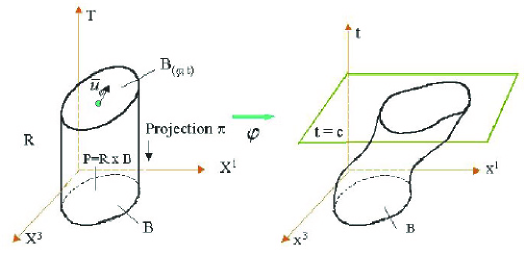
Figure 1. 4D Deformation History and the Field of Flow Vector

A deformation history $\phi$ for which $t=\phi^{0}(X)=T$ will be called ”synchronized”. The synchronization can practically performed for relatively slow deformation processes (in comparison to sound wave velocity).

Using the deformation $\phi$, we introduce the slicing of the material space-time $P$ by the level surfaces of the zeroth component of $\phi$

$$B_{\phi}=\{B_{\phi,t}=\phi^{0\ -1}(t)\}=\{(T,X)\in P|\phi^{0}(T,X)=t\}.$$ (2.1)

For a synchronized deformation $B_{\phi,t}=\{(T,X)\in P|T=t\}.$

There is a time flow vector field $u_{\phi}$ in $P$, associated with the slicing $B_{\phi,t}$ of the space-time $P$ ([4], [7]). This (future directed) vector field represent the flow of ”intrinsic” (proper in Relativity Theory) time in the material. Lifting the index in the 1-form $d\phi^{0}$ with the help of the metric $G$ and normalizing obtained vector field, we define the time flow vector field as

$$u^{.}_{\phi}=\frac{(d\phi^{0})^{\#}}{\|d\phi^{0}\|}_{G}.$$ (2.2)

The norm of the 1-form $d\phi^{0}$ is defined as $\|d\phi^{0}\|^{2}=(G^{AB}\phi^{0}_{,A}\phi^{0}_{,B})^{1/2}$ (summation agreement by repeating indices is used here). Thus, $u_{\phi}$ is the unit vector $G$-orthogonal to the slices $B_{\phi,t}$. In the local coordinates $X^{I}$,

$$u^{.}_{\phi}=\frac{G^{AB}\phi^{0}_{,B}}{\sqrt{G^{AB}\phi^{0}_{,A}\phi^{0}_{,B}}}\frac{\partial}{\partial X^{A}}.$$ (2.3)

For the synchronized deformations does not depend on $\phi$:

$$u^{.}_{\phi}=u^{.}_{G}=\frac{G^{I0}}{\sqrt{G^{00}}}\frac{\partial}{\partial X^{I}}.$$ (2.4)

Additionally, if the metric $G$ has the block-diagonal form in the coordinates $(X^{0}=T,X^{I})$ (shortly, BD - metric), we have $u^{.}_{G}=[G_{00}]^{-\frac{1}{2}}\frac{\partial}{\partial T}.$

Let $u_{0}=\frac{\partial}{\partial T}$ be the flow vector associated with the metric $G_{0}$ and the corresponding 3D slicing $B_{0}$.

We require fulfillment of the following condition ensuring the irreversibility of the flow of time:

$$<u_{\phi},u_{0}>_{G}\ >0.$$ (2.5)

Deformation history $\phi$ for which the condition (2.5) is satisfied is called admissible.

In coordinates $(X^{I})$ this condition reduces to the following simple inequality

$$\phi^{0}_{,0}>0$$ (2.6)

and, therefore is a restriction on the deformation history only.

For a synchronized deformation history $\phi$, this condition is trivially satisfied.

Time component $\phi^{0}$ of the deformation history may be excluded from the list of dynamical variables by an appropriate ”gauging”. Namely, we use the invariance of Lagrangian under the automorphisms of the bundle $(P,\pi,B)$ to make the deformation history synchronized.

An automorphism $F:P\longmapsto P,X^{I}=F^{I}(Y^{A})$ of the bundle $(P,\pi,B)$ determines the diffeomorphism of the base $B$ that can be considered as a change of variables $X^{I}=F^{I}(Y^{A})$.

In the new variables, the condition (2.6) takes the form $\frac{\partial\phi^{0}}{\partial Y^{0}}=\phi^{0}_{,I}F^{I}_{,0}=\phi^{0}_{,0}F^{0}_{,0}>0$ (since $F^{I},\ I=1,2,3$ do not depend on $Y^{0}$). Thus, the class of admissible deformation histories $\phi$ is stable under the action of the subgroup $Aut^{+}(P)$ of all automorphisms of $P$ with $F^{0}_{,0}>0$.

The group $Aut^{+}(P)$ of automorphisms of the bundle contains two subgroups. One is the subgroup $TC$ of the ”time change” proper gauge diffeomorphisms $(X^{0}=T;X^{I},I=1,2,3)\longmapsto(F(T,;X^{J},J=1,2,3),X^{I},I=1,2,3)$ for an arbitrary smooth function $F(X^{I})$ with $F_{,0}>0.$ The other one (denoted $D(B)$) consists of the lifts to the slices $B_{\phi,t}$ of the manifold $P$ of the orientation preserving diffeomorphisms of the base $B$ (group of such transformations of $B$ is denoted $Diff^{+}(B)$). To lift a diffeomorphism we use (diffeomorphic) projections $\pi_{\phi,t}=\pi|_{B_{\phi,t}}:B_{\phi,t}\longmapsto B$. If $\phi$ is synchronized, lifted diffeomorphisms do not depend on $T$.

Any automorphism of the bundle $\phi\in Aut^{+}(P)$ generates the time independent diffeomorphism $\phi_{B}$ of the base $B$, that is element of $Diff^{+}(B).$ Lifting this element to the element of $D(B)$ we represent the group $Aut^{+}(P)$ as the semi-direct product of the normal subgroup $TC(P)$ and the subgroup $D(B)$. Thus, we have proved the first of two following statements

1. Automorphisms group $Aut^{+}(P)$ is the semidirect product of the subgroup $D(B)\sim Diff^{+}(B)$ of orientation preserving diffeomorphisms of the base $B$ and the subgroup $TC$ of proper gauge transformations $\xi_{F}$ of the fibers

   $$\xi_{F}:((X^{0}=T;X^{I},I=1,2,3)\longmapsto(F(T,;X^{J},J=1,2,3),X^{I},I=1,2,3))$$

   with $F_{,0}>0.$

2. For any admissible history of deformations $\phi$ one can choose a transformation $\xi_{F}\in TC$ such that the history of deformation $\phi\circ\xi_{F}$ is synchronized.

To prove the second statement let $\phi$ be an admissible history of deformation. Define the element $F\in TC(P)$ as follows: $F:(T,X^{I},I=1,2,3)\longmapsto(\phi^{0}(T,X^{J},J=1,2,3),X^{I},I=1,2,3)$. Then, $\phi=\phi_{1}\circ F$ where $\phi_{1}$ is another admissible history of deformation with the same components $\phi^{i},i=1,2,3$ and the identity component $\phi_{1}^{0}(T,X^{I},I=1,2,3)=T$. Transformation $F$ is admissible since $F^{0}_{,0}=\phi^{0}_{,0}>0$, thus $F\in TC(P).$ Apparently, the deformation history $\phi_{1}$ is synchronized.

Therefore we may restrict our consideration to the synchronized histories of deformation keeping in mind that the covariance group of the theory reduces from the group $Aut^{+}(P)$ to the group $D(B)$ of time-independent orientation preserving diffeomorphisms of base $B$.

2.3. ADM-decomposition of Material Metric, Lapse and Shift.

Slicing $B_{\phi,t}$, generates the (3,1)-decomposition of the material metric $G$ employed (for a Lorentz type metric) in General Relativity ([4],[5]). Specifically, the sandwich structure of the part of the manifold $P$ bounded by the surfaces $B_{\phi,t}$ and $B_{\phi,t+\Delta t}$ allows one to introduce the time-dependent lapse function $N$ and the shift vector field $\vec{N}$ tangent to the slices $B_{\phi,t}$ such that the metric is block-diagonalized in the moving coframe $(dT,dX^{A}+N^{A}dT)$:

$$ds^{2}=G_{IJ}dX^{I}dX^{J}=g_{IJ}(dX^{I}+N^{I}dT)(dX^{J}+N^{J}dT)+S^{2}dT^{2}.$$ (2.7)

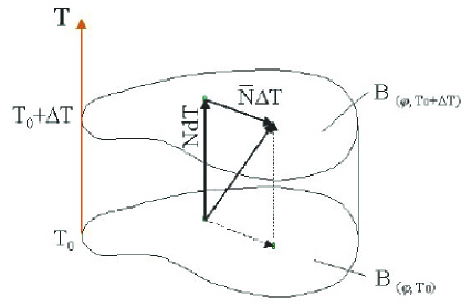
Figure 2. Lapse Function $S$ and Shift Vector $\vec{N}$.

Matrix representation of the material metric tensor $G$ and inverse tensor $G^{-1}$ have in these notations, the forms

$$\left(\begin{array}[]{cc}G_{00}&G_{0J}\\ G_{I0}&G_{IJ}\end{array}\right)=\left(\begin{array}[]{cc}N_{A}N^{A}+S^{2}&N_{J}\\ N_{I}&g_{IJ}\end{array}\right),\ \ \left(\begin{array}[]{cc}G^{00}&G^{0J}\\ G^{I0}&G^{IJ}\end{array}\right)=\left(\begin{array}[]{cc}\frac{1}{S^{2}}&-\frac{N^{J}}{S^{2}}\\ -\frac{N^{I}}{S^{2}}&g^{IJ}+\frac{N^{I}N^{J}}{S^{2}}\end{array}\right),$$ (2.8)

where $g$ is the 3D-metric induced by $G$ on the slices $B_{\phi,t}$ and $g^{-1}$ is the corresponding inverse tensor. In these notations $\sqrt{|G|}=S\sqrt{|g|}.$

In what follows we assume that the 4D-deformation history $\phi$ is synchronized. Thus slices $B_{\phi,t}$ has the form $T=t=const$.

In these notations, the flow vector $u_{G}$ and the corresponding 1-form have the form

$$u_{G}=\frac{1}{S}\partial_{T}-\frac{N^{A}}{S}\partial_{X^{A}},\ \ u_{G}^{\flat}=SdT.$$ (2.9)

The last formula gives the ”material time differential” $d\tau=SdT$ for the material metric $G$. In our context, the coordinate X dependence of lapse function S(T,X) accounts for heterogeneity of material aging in different points of the solid. On the Fig. 3 the local observer at different points of body at different moments of time $T$ sees the different rate of the local time in comparison with the laboratory clocks.

Moreover, the lapse function S can be considered as an intrinsic measure of material age, associated with its cohesiveness. It can be normalized to be equal 1 in the reference state of the solid. As a result of energy dissipation in various inelastic processes, material loses its cohesiveness with aging. In the formalism presented here it is manifested in slowing down of the material (intrinsic) time, i.e. increasing of $S(X,T)$.

Here we do not consider thermodynamics. However, monotonic increase of $S(X,T)$ resembles and can be linked to the principle of non-negative entropy production of the thermodynamics of irreversible processes: $\frac{dS_{in}}{dt}>0.$

The requirement $S>1$ leads to the strong constraints on the form of the ”ground state term” of the material Lagrangian $L_{m}$, (see Sec. 5).

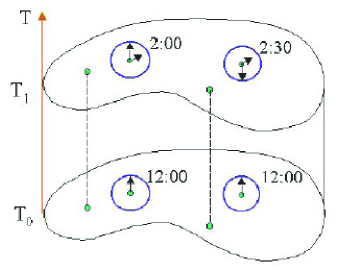
Figure 3. Illustration of Time Rate $S$ (Lapse Function) by Variation of Time Interval $(\tau-\tau_{0})=S(T_{1}-T_{0}).$

In this context, the shift vector field $\vec{N}$ in the metric $G$ reflects a propagation of the phase transition or chemical transformation boundary through the material as reflected, for instance in the mass conservation law (see below).

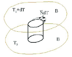
Figure 4. Propagation of Phase Boundary Represented by Shift Vector $\vec{N}$

The separation of the evolution of 3D material metric $g$, material transformation process in $B_{t}$, characterized by $\vec{N}$ and the inhomogeneity of the local time $d\tau=SdT$, are the main reason for introduction (3+1) ADT-representation of 4D-metric in Gravity Theory ([4]). In addition, an adoption of this view leads to a very clear separation of the ”physical” degrees of freedom in the canonical formalism and to the explicit hyperbolic formulations of Einstein Equations ([10, 11]).

3. Mass conservation law

The mass form $dM=\rho_{0}dV$ defined in P is introduced here, in addition to the volume form $dV_{G}$ of metric $G$. The reference mass density $\rho_{0}$, defined by this representation, satisfies the mass conservation law ([6],[7])

$${\mathcal{L}}_{u_{\phi}}dM=d(i_{u_{\phi}}dM)=0.$$ (3.1)

Here ${\mathcal{L}}_{u_{\phi}}$ is the Lie (substantial) derivative of the exterior 4-form $dM$ in the direction of the vector field $u_{\phi}$. Recall that the Lie derivative of a differential form $\omega$ along a vector filed $u$ is defined as ${\mathcal{L}}_{u}\omega=\frac{d}{dt}\phi^{*}_{t}\omega|_{t=0},$ where $\phi^{*}_{t}\omega$ is the pullback of the form $\omega$ by the flow $t\longrightarrow\phi_{t}=exp(tu)$ of the vector field $u$ ([6]).

Equation (3.1) is equivalent to the condition $div_{G}(\rho_{0}u_{\phi})=0$, where divergence is taken with respect to the volume form $dV$. In local coordinates the Mass Conservation Law has the form

$$\left(\frac{G^{IB}\phi^{0}_{,B}}{\|d\phi^{0}\|}\rho_{0}\sqrt{|G|}\right)_{,I}=0.$$ (3.2)

Due to the properties of the metric $G$ and the deformation $\phi$, the material space-time manifold $P$ is foliated by the phase curves of the flow vector field $u_{\phi}$ and thus the value of the reference mass density $\rho_{0}(0,X)$ at $T=0$ uniquely defines its values for all $T>0$.

In the synchronized case $\phi^{0}=T,\|d\phi^{0}\|=\sqrt{G^{00}}=S^{-1},\ G^{M0}=-\frac{N^{M}}{S^{2}},\ G^{00}=S^{-2}$ and (3.2) take the form of the following balance law

$$(\rho_{0}\sqrt{|g|})_{,0}=\sum_{A=1}^{3}\left(N^{A}\rho_{0}\sqrt{|g|}\right)_{,A}.$$ (3.3)

From (3.3) we note that the shift vector field $\vec{N}$ can describe the matter (density) flow due to the some internal processes such as the phase or chemical transformations.

If, in addition to being synchronized, the material metric $G$ is also in the BD-form ($\vec{N}=0$), the flow term in (3.3) disappears and the mass conservation law is equivalent to the following representation of the reference mass density in terms of its initial value $\rho_{0}(0,X)=\rho_{0}$:

$$\rho_{0}(T,X^{I})=\rho_{0}(0,X)\sqrt{\frac{G_{00}}{|G|}}=\frac{\rho_{0}(0,X)}{\sqrt{|g(T,X)|}},$$ (3.4)

where $G(0,X)$ is assumed to be Euclidean metric. If metric $G$ does not changes with time $T$, we get the classical local mass conservation law $\frac{\partial\rho_{0}}{\partial T}=0.$

4. Elastic, Inelastic and Total Strain Tensors

In this section we introduce the principal quantities characterizing both elastic and inelastic deformation processes. Total deformation is presented as a composition of elastic and inelastic ones and is integrable. Its elastic and inelastic ”components” are non-integrable, in general, but might be such in special situations (see Sec.11). We recall that the presentation of total deformation as a composition of this type was studied in different forms in many works ([9, 12, 14], to name a few). What is new here is the 4D-approach to this decomposition and direct definition of elastic, inelastic and total strain tensors in terms of material metric $g_{t}$ as an independent dynamical variable, reference (undeformed) Cauchy metric $g_{0}$ and the current Cauchy metric $C_{3}(\phi)$ rather then using the ”deformation gradients” (integrable or not) of elastic and inelastic (plastic) deformations.

Slicing $B_{\phi\ ,t}$ of $P$ defines the covariant tensor $\gamma=G-u_{\phi}\otimes u_{\phi}=^{s}\left(\begin{array}[]{cc}N_{A}N^{A}&N_{J}\\ N_{I}&g_{IJ}\end{array}\right)$ ([7],[4]). Here and later the sign $s$ over $=$ means that this equality is true in synchronized case. Tensor $\gamma$ induces the time dependent 3D-metric $g_{t}$ on the slices $B_{\phi\ ,t}$ (see, for example, [11]).

To obtain the expression for $g_{t}$ in material coordinates $X^{I}$, we notice that the tangent vectors

$$\xi_{I}=-\frac{\phi^{0}_{,I}}{\phi^{0}_{,0}}\partial_{X^{0}}+\partial_{X^{I}},\ I=1,2,3$$ (4.1)

form the basis of the tangent spaces to the slices $B_{\phi,t}.$ In this basis, $g_{t}$ is given by

$$g_{AB}=g(\xi_{A},\xi_{B})=G_{AB}-G_{0B}\frac{\phi^{0}_{,A}}{\phi^{0}_{,0}}-G_{A0}\frac{\phi^{0}_{,B}}{\phi^{0}_{,0}}+G_{00}\frac{\phi^{0}_{,A}\phi^{0}_{,B}}{\phi^{0\ 2}_{,0}},\ A,B=1,2,3.$$ (4.2)

For a synchronized deformation $\gamma=G-(G^{00})^{-1}dT\otimes dT$ and $g_{t}$ is simply the restriction of 4D-metric $G$ to the slices $B_{T=c}$, i.e. $g_{t\ IJ}=G_{IJ}|_{T=t}$, see (2.8).

Denote by $h_{t}$ the 3D metric on the leaves $B_{\phi,t}$ induced by the metric $G_{0}$ (that is by the tensor $\gamma_{0}=G_{0}-u_{0}\otimes u_{0}$).

Associated with the tensor $\gamma$ there is the projector ((1,1)-tensor)

$$\Pi=G^{-1}\gamma=I-u^{*}_{\phi}\otimes u_{\phi}=^{s}\ I-\frac{G^{I0}}{G^{00}}\partial_{X^{I}}\otimes dT=\left(\begin{array}[]{cc}0&0\\ N^{I}&I_{3}\end{array}\right).$$ (4.3)

on the tangent spaces to the slices $B_{\phi,t}$, last equality being true for synchronized deformations $\phi$.

Let us consider the pullback $\ C_{4}(\phi)=\phi^{*}\hat{h}$ of the degenerate tensor $\hat{h}$ by the 4D-deformation mapping $\phi$. Tensor $C_{4}(\phi)$ is degenerate in $P$, its kernel is generated by the vector $\phi^{-1}_{*}(\frac{\partial}{\partial t})$. In coordinates $(X^{I})$ we have

$$C_{4}(\phi)_{IJ}=\left(\begin{array}[]{cc}h_{ij}\phi^{i}_{,0}\phi^{j}_{,0}=\|\mathbf{V}\|^{2}_{h}&h_{ij}\phi^{i}_{,0}\phi^{j}_{,J}\\ h_{ij}\phi^{i}_{,I}\phi^{j}_{,0}&\sum^{3}_{i,j=1}h_{ij}\phi^{i}_{,I}\phi^{j}_{J}\end{array}\right).$$ (4.4)

The spatial part of this tensor is the conventional Cauchy-Green strain tensor $C_{3}(\phi)$ of the Elasticity Theory. Components of this tensor with indices (0J) and (I0), $I,J=1,2,3$ have the form velocity $\times$  deformation covector (see [15]). (00)-component of $C_{4}(\phi)$ is the square of the material velocity $\mathbf{V}=\phi_{3*}(\frac{\partial}{\partial T})=^{s}\frac{\partial\phi^{i}}{\partial t}\frac{\partial}{\partial x^{i}}$.

4.1. Elastic Strain Tensor

Here we define the 4D (1,1)-elastic strain tensor in $P$. We will do it first in linear approximation and then, using logarithm of a (1,1)-tensor function, in another way, more suitable for large deformations.

We start with the following, conventional definition:

$${\hat{E}}^{el\ \cdot}_{\cdot}=\frac{1}{2}G^{-1}(C_{4}(\phi)-\gamma)=^{s}\\ =\frac{1}{2}\begin{pmatrix}S^{-2}\|\mathbf{V}\|^{2}_{h}-S^{-2}N^{I}\langle\mathbf{V},\phi^{.}_{,I}\rangle_{h}&S^{-2}\langle\mathbf{V},\phi^{.}_{,J}\rangle_{h}-S^{-2}N^{K}\langle\phi^{.}_{,K}\phi^{.}_{,J}\rangle_{h}\\ -S^{-2}N^{I}\|\mathbf{V}\|^{2}_{h}-N^{I}+&-S^{-2}N^{I}\langle\mathbf{V},\phi^{.}_{,J}\rangle_{h}+g^{IK}C_{3}(\phi)_{KJ}-\\ +(S^{-2}N^{I}N^{K}+g^{IK})\langle\phi^{.}_{,K},\mathbf{V}\rangle_{h}&-\delta^{I}_{J}-S^{-2}N^{I}N^{K}\langle\phi^{.}_{,K}\phi^{.}_{,J}\rangle_{h}\end{pmatrix}.$$ (4.5)

This tensor contains the square of material velocity and the shift vector field. Having in mind the general, dynamical situation it is more appropriate to use the following tensor as the proper Elastic Strain Tensor

$$E^{el\ .}_{.}(\phi)=\Pi{\hat{E}}^{el}\Pi=\frac{1}{2}\Pi G^{-1}(C_{4}(\phi)-\gamma))\Pi=^{s}\frac{1}{2}\left(\begin{array}[]{cc}0&0\\ g^{IK}\langle\phi^{.}_{,K},\phi^{.}_{,0}\rangle_{h}-N^{I}&g^{IK}C_{3}(\phi)_{KJ}-\delta^{I}_{J}\end{array}\right),$$ (4.6)

Here $\Pi$ is the projector on the slices $B_{\phi,t}$ defined in (4.3). The last equality is valid in the synchronized case. Notice that the basic invariants $Tr(A^{k})$ for the tensor (4.6) are the same as for the tensor $C_{3}(\phi)-g$.

For the simplicity we use the same symbol $E^{el}$ for the restriction of this tensor to the slices $B_{\phi,t}$.

Tensor $E(\phi)^{el}$ is a measure of the deviation of the Cauchy metric $C_{3}(\phi)$ of the actual state from the ”ground state” $G$. For a synchronized deformation $\phi$ and a material metric $G$ with the zero shift vector, $E^{el}=\frac{1}{2}(C(\phi)-g_{t})$ has the form of the conventional elastic strain tensor.

Remark 1.

The deformation $\phi$ is essentially 3-dimensional in the sense that only the spatial Euclidean metric $g_{0}=h$ in $B$ is deformed. The 4D-tensor $C_{4}(\phi)=\phi^{*}h$ defines the degenerate metric in the material space-time $P$. It is instructive to compare $C_{4}(\phi)$ with the (degenerate) tensor $\gamma=G-u_{\phi}\otimes u_{\phi}$. The elastic strain tensor $E^{el}$ measures the deviation of $C_{4}(\phi)$ from $\gamma$ on the slices $B_{\phi,t}$. Thus, the scheme presented here is essentially different from relativistic elasticity theory ([7],[8]) as well as from 4D version of conventional elasticity theory.

We see from (4.6) that $E^{el}=0$ if and only if the following two conditions are fulfilled:

$$\begin{cases}1)\ g_{ij}=C_{3}(\phi)_{IJ}=\phi_{3}^{*}(h)_{IJ},\\ 2)\ N^{I}=g^{IK}\langle\phi^{.}_{,0},\phi^{.}_{,K}\rangle.\end{cases}$$ (4.7)

In particular, metric $g$ coincide with the Cauchy metric induced by deformation $\phi$ and is flat.

If $E^{el}=$ then ${\hat{E}}^{el}=0$ if and only if in addition to the conditions (4.9) the following conditio is fulfilled

$$3)\ \|V\|^{2}_{h}=g^{IJ}\langle\phi^{.}_{,0},\phi^{.}_{,I}\rangle\langle\phi^{.}_{,0},\phi^{.}_{,J}\rangle.$$ (4.8)

4.2. Inelastic Strain Tensor

Now we introduce the inelastic strain tensor in linear approximation

$${\hat{E}}^{in}=\frac{1}{2}G^{-1}(\gamma-\gamma_{0})=^{s}\frac{1}{2}\left(\begin{array}[]{cc}0&S^{-2}N^{K}h_{KJ}\\ N^{I}&\delta^{I}_{J}-g^{IK}h_{KJ}-S^{-2}N^{I}N^{K}h_{KJ}\end{array}\right),$$ (4.9)

(last equality being true in synchronized case) and the total strain tensor ${\hat{E}}^{tot}$ of the body at each given moment $T$ to characterize the deviation of the deformed Euclidean metric $\phi^{*}h|_{B_{\phi,t}}$ from the initial (Euclidean) 3D-metric $h$ ($h$ being the restriction of $G_{0}$ to the slices $B_{\phi,t}$)

$${\hat{E}}^{tot}=\frac{1}{2}G^{-1}(C_{4}(\phi)-\gamma_{0}).$$ (4.10)

Tensor ${\hat{E}}^{tot}$ can be represented as the sum of the elastic strain tensor ${\hat{E}}^{el}$ and of inelastic strain tensor ${\hat{E}}^{in}$:

$${\hat{E}}^{tot}={\hat{E}}^{el}+{\hat{E}}^{in}.$$ (4.11)

To obtain the corresponding decomposition for the 3D strain tensors we apply projector $\Pi$ to the total and inelastic strain tensors. In particular we introduce

$$E^{in}=\Pi{\hat{E}}^{in}\Pi=^{s}\frac{1}{2}\left(\begin{array}[]{cc}0&0\\ N^{I}-g^{IK}h_{KB}N^{B}&\delta^{I}_{J}-g^{IK}h_{KJ}\end{array}\right),$$ (4.12)

As a result, we get from (4.11) the corresponding decomposition of ”3D total strain tensor”

$$\Pi E^{tot}\Pi=E^{el}+E^{in}.$$ (4.13)

Restriction of these tensors on the 3D slices $B_{\phi,t}$ leads to the more conventional ($t$-dependent) version of this decomposition.

For a synchronized deformation history, restriction of $E^{in}$ to the slices $B_{t}$ takes the form

$$E^{in}|_{B_{t}}=\frac{1}{2}g^{-1}(g-g_{0})=\frac{1}{2}(I-g^{-1}g_{0}),$$ (4.14)

that describes the decline of 3D material metric $g$ from its initial (reference) value $g_{0}=\phi^{*}_{0}h$.

Another way to define strain tensors, more suitable for description of large deformation is to take

$${\hat{E}}^{el}=\frac{1}{2}ln(G^{-1}C_{4}(\phi))),{\hat{E}}^{in}=\frac{1}{2}ln(G^{-1}_{0}G)),{\hat{E}}^{tot}=\frac{1}{2}ln(G^{-1}_{0}C_{4}(\phi))).$$ (4.15)

We can define $E^{el},\ E^{in},\ E^{tot}$ correspondingly, using projector $\Pi$. Strain tensors, defined in such a way will, in some simple cases, enjoy the same additive relations as (4.11),(4.13). On the other case, if elastic deformation happens in the directions different from the principal axes of inelastic deformation, relation between these deformations becomes more complex.

The relationship between these definitions and those of the linear approximation above is established by using the fact that for a couple $A,B$ of (0,2)-tensors such that $A$ is invertible, $ln(A^{-1}B)\approx A^{-1}(A-B)$ provided $A-B$ is small enough. Thus, when linear approximation is allowable, first definition is the good approximation of the second. For instance

$$ln(g^{-1}C_{3}(\phi))=ln(I+g^{-1}(C_{3}(\phi)-g))\approx g^{-1}(C_{3}(\phi)-g),$$ (4.16)

provided $C_{3}(\phi)-g$ is small.

4.3. Strain Rate Tensor

One can also define the material elastic strain rate tensor as follows

$${\dot{\hat{E}}}^{el}={\mathcal{L}}_{u_{\phi}}{\hat{E}}^{el},$$ (4.17)

as well as inelastic strain rate tensor

$${\dot{\hat{E}}}^{in}={\mathcal{L}}_{u_{\phi}}{\hat{E}}^{in}.$$ (4.18)

In the case where $G=G_{0}$ and $\phi^{0}=T$, elastic strain rate tensor defined in (4.17) has, the same spatial components as the conventional strain rate tensor ([6]).

Denote by $\dot{G}$ the the Lie derivative ${\dot{G}}={\mathcal{L}}_{u_{\phi}}G$ of the metric tensor $G$ with respect to the flow vector $\vec{u}_{\phi}$. Then the calculation of the Lie derivative in (4.17) results in the following relation

$${\dot{\hat{E}}}^{el}={\mathcal{L}}_{u_{\phi}}{\hat{E}}^{el}=-G^{-1}{\dot{G}}{\hat{E}}^{el}+\frac{1}{2}G^{-1}({\dot{C_{4}(\phi)}}-{K}),$$ (4.19)

where $K={\mathcal{L}}_{u_{\phi}}\gamma$ is the extrinsic curvature tensor of the slices $B_{\phi,t}$.

Remark 2.

Here we are using material coordinates and tensors only. In order to obtain the corresponding ”laboratory” quantities (seen by an external observer), one defines the laboratory (Euler) Elastic Strain Tensor

$$\epsilon^{el\ i}_{j}=\phi^{i}_{,A}\phi^{-1\ B}_{j}E^{el\ A}_{B}$$ (4.20)

and recalculate all the other quantities accordingly.

Figure 5 presents the above decomposition of total deformation into the inelastic and elastic deformations.

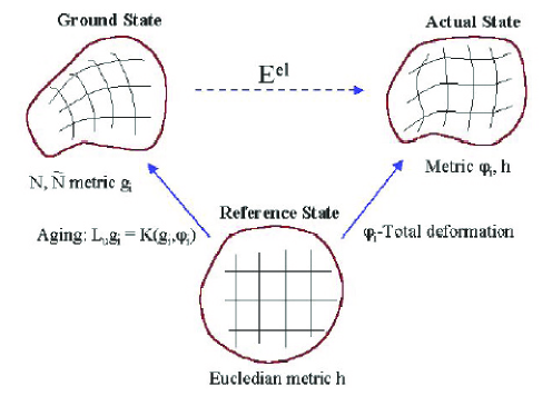
Figure 5. Decomposition of Deformation History.

The actual state under the load at any given moment $T$ results from both elastic (with the variable elastic moduli) and inelastic (irreversible) deformations. The ”ground state” of the body is characterized by the 3D-metric $g_{t}$. This state is the background to which the elastic deformation is added to reach the actual state ([14]).

Transition from the reference state to the ”ground state” that manifests in the evolution of the (initial) Euclidean metric $h$ to the metric $g_{t}$ cannot be described, in general, by any point transformation. Transition from the ”ground state” to the actual state at the moment $t$ also is not compatible in general. Yet the transition from the reference state to the actual state is represented by a diffeomorphism $\phi_{t}$.

Here we are considering the material 4D-metric $G$ and the deformation $\phi$ (or elastic strain tensor $E^{el}(\phi)$) to be the dynamical variables of the field theory. The reference mass density $\rho_{0}$ is found (for the synchronized deformation $\phi$ and the BD-metric $G$) by the formula (3.4) if its initial value $\rho_{0}(T=0)$ is known. In this study we consider mainly the quasi-static version of the theory, i.e. inertia forces and kinetic energy are assumed to be negligible.

5. Parameters of Material Evolution, metric Lagrangian

In examining the processes of deformation and aging of a solid with a synchronized deformation history $\phi$ we use both general $(G_{IJ})$ and ADM ($S,\vec{N},g$) notations for the 4D material metric $G$.

Following the framework of Classical Field Theory ([16]) we take a Lagrangian density ${\mathcal{L}}(G,\phi)$ referred to the volume form $dV$ as a function of 4D-material metric $G$, its invariants (with respect to the group of $Diff^{+}(B)$ of the orientation preserving diffeomorphisms of the base $B$, see above) and the elastic strain tensor: $L(G,E^{el})$.

The Lagrangian $L(G,E^{el})dV$ is represented as a sum of the two parts: the metric part $L_{m}(G)$ and, as a perturbation of the ground state, the elastic part $L_{e}(G,E^{el})$ associated with elastic deformation

$$L=L_{m}(G)+L_{e}(E^{el},G).$$ (5.1)

Metric Lagrangian $L_{m}(G)$ in (5.1) is introduced to account for the ”cohesive energy” or strength of the solid state, the strain energy of ”residual strain” and the energy of the change associated with a evolution of material properties in time, for instance material aging processes of phase transitions.

Metric Lagrangian $L_{m}$ is the sum of several terms with the coefficients that may depend on the 3D volume factor $|g_{t}|$ (actually $|g_{t}|/|g_{0}|$) and the lapse function $S$. These volume factors are associated with the solid state ability to retain its intrinsic topology in contrast to the fluid and gaseous states.

First term of $L_{m}$ is the ”ground state energy” $F(E^{in},S,\|\vec{N}\|^{2}_{g})$ (shortly GS) - initial (”cohesive”) energy (per unit volume).

The second (kinetic) term in $L_{m}$ (see (5.4) below) is the function of invariants of the tensor $K={\mathcal{L}}_{u_{G}}\gamma$ of extrinsic curvature of the slices $B_{T}$ in the material space-time $P$ ( [4, 11]).

In the ADM notations, the (1,1)-tensor $K$ has the following form

$$(K^{I}_{J})=\left(\begin{array}[]{cc}0&0\\ (*)&S^{-1}g^{IS}(\xi\cdot g)_{SJ}\end{array}\right),$$ (5.2)

where $(*)$ represents the terms which do not enter the invariants of $K$ and $\xi\cdot g=\frac{\partial}{\partial T}g-{\mathcal{L}}_{\vec{N}}g$. Lie derivative ${\mathcal{L}}_{\vec{N}}g$ of the tensor $g$ with respect to the vector field $\vec{N}$ is calculated on each 3D slice $B_{T}$ for a fixed $T$.

In the case of a block-diagonal metric $G$ (no shift: ${\bar{N}}=0$), $\gamma=\left(\begin{array}[]{cc}0&0\\ 0&g_{t}\end{array}\right)$; therefore, $K$ is, essentially, the time derivative of the metric $g_{t}$:

$$K^{I}_{J}=\left(\begin{array}[]{cc}0&0\\ 0&S^{-1}g^{IA}\frac{\partial}{\partial T}g_{AJ}\end{array}\right).$$ (5.3)

Therefore, tensor $K$ represents the rate of change of intrinsic length scales that reflects the aging processes. It shall be noted that $K$ is also related to the elastic strain rate (see (4.19)).

$L_{m}(G)$ also may depend on the shift vector field $\vec{N}$ through its norm $\|\vec{N}\|_{g}^{2}=N_{A}N^{A}$ (entering the ”ground state energy” $F$) and, possibly, divergence $div_{g}({\vec{N}})$ and the ”proper time derivative” ${\mathcal{L}}_{u}{\vec{N}}$.

We also include the term reflecting the residual strain energy (incompatibility) of $E^{tot}$ which is accounted for by the scalar curvature $R(g)$ of 3D material metric $g$.

Summarizing the above assumptions we construct the metric Lagrangian $L_{m}$ as the scalar function of the parameters listed above:

$$L_{m}=F(S,\|\vec{N}\|^{2}_{g},E^{in})+\chi(K)+\alpha div_{g}(\vec{N})^{2}+\beta R(g_{t}).$$ (5.4)

Function $\chi$ of invariants of tensor $K^{I}_{J}$ (”dissipative potential”, comp.[13]) corresponds to the energy of inelastic processes in the material .

Coefficients $\alpha,\beta$ may depend on $S$ and $|g|$.

In the case of a homogeneous media or in 1D case, the scalar curvature $R(g_{t})$ of the metric $g_{t}$ is zero and the corresponding term in (5.4) vanishes.

Given the diversity of the material properties and the different conditions (of loading, boundary, forces, heat,etc.) of inelastic processes affecting the material it is especially important to choose the material Lagrangian of different materials appropriately. It appears as if the different conditions activate different ”layers” of structural changes for a given material and, correspondingly, turn on terms in the ”ground energy” and in the ”dissipative potential” that are responsible for the given type of aging. For example, the slow process of unconstrained aging in a homogeneous rod (see sec.11. or [19]) is overcome by the scale processes of a stress relaxation or creep each of which begins in a different loading situation after the strain energy (density) reaches a (different) activation level. For these two processes both ground energy $F$ and the dissipative potential $\chi(K)$ have the same form different from those for unconstrained aging.

Remark 3.

The scalar curvature $R(G)$ of the 4D metric $G$ can be expressed, by the Gauss equation, as the combination of scalar curvature of 3D metric $g$ and of invariants of its extrinsic curvature: $R(G)=-(tr({K}^{2})-(trK)^{2})+R(g_{t})$, up to a divergence term ([11]). As a result, the above form of Lagrangian for an aging media (5.4) is a generalization of the Hilbert-Einstein Lagrangian $R(G)\sqrt{|G|}$ of the General Relativity ([4]). By breaking of the invariance group of general relativity to the smaller group of automorphisms of the bundle $P\rightarrow B$ we can use more general form of metric Lagrangian.

The perturbation of Lagrangian due to elastic deformation is taken in the form of the Lagrangian of Classical elasticity ([6], Sec.5.4)

$$L_{e}(E^{el},G)=\frac{\rho_{0}}{2}\|V\|^{2}_{h}-\rho_{0}f(E^{el},G)-\rho_{0}U\circ\phi,$$ (5.5)

where $\rho_{0}\|V\|^{2}_{h}=\rho_{0}\sum_{ij}h_{ij}\phi^{i}_{,0}\phi^{j}_{,0}$ is the density of kinetic energy, $f$ is the strain energy per unit of mass, $U$ is the potential of the body forces. Strain energy $f$ is assumed to be a function of two first invariants of the (1,1)-strain tensor $E^{el}$. Strain energy may depend on the metric $G$ through the invariants of $g_{0}^{-1}g_{t},\ S$, vector field $\vec{N}$, scalar curvature $R(g)$ etc.

Because we are considering a quasistatic synchronized theory here we ignore the inertia effects and, therefore, omit the kinetic energy term in (5.5).

The strain energy density in linear elasticity is conventionally presented as follows

$$f(E^{el})=\frac{\mu}{2}Tr(E^{el\ 2})+\frac{\lambda}{2}(Tr(E^{el}))^{2},$$

where $\mu,\lambda$ are the initial values of the Lame constants ([18]).

We assume that Strain Energy $f$ and the ”ground state” term $F$ are independent of each other. Yet, in Appendix A we introduce a scheme where elastic deformation (elastic strain tensor $E^{el}$) is considered as (small) perturbation of (large) inelastic deformation (presented by inelastic strain tensor $E^{in}$). Therefore, strain energy $f(E^{el})$ is obtained by decomposition of the function $F(S,E^{tot})$ into the ”Taylor series” by the parameter $E^{el}$. This leads to the expression of elastic moduli of a media through the invariants of material metric $g$ and the lapse function $S$.

6. Action, boundary term, Hooke’s law.

The Action functional is the integral of the Lagrangian density $\mathcal{L}(G,\phi)$ over a 4D domain $U=[0,T_{0}]\times V$. Here $(V,\partial V)$ is an arbitrary subdomain of $B$ with the boundary $\partial V$, combined with the 3D boundary integral that accounts for the work $W$ of surface traction ([6]).

$$A_{U}(G,\phi)=\int_{U}(L_{m}(G)+L_{e}(E^{el},G))dV+\int_{[0,T_{0}]\times\partial V_{1}}V_{\tau}(\phi,G)d^{3}\Sigma.$$ (6.1)

Here $d^{3}\Sigma$ is the area element on the 3D boundary $\partial U$ of the cylinder $U$ ([6]).

The second term on the right represents a boundary conditions put on the deformation history $\phi$. Typically the boundary $\partial V$ of the domain $V\subset B$ is divided into two parts $V=\partial V_{1}\cup\partial V_{2}$. The deformation is prescribed on the part $\partial V_{2}$: $\phi_{\partial V_{2}}=\psi(t,X),$ while along the part ${\partial U_{1}}$ of the boundary the traction $\tau$ is prescribed. Function $V_{\tau}$ depends (conventionally) on the velocity $\vec{V}$ of deformation $\phi$ and on the traction 1-form $\tau$, which is chosen in such a way as to have $-\nabla_{\phi}V_{\tau}=\tau$ - traction ([6]). In Euclidean space with the dead load one takes $V_{\tau}=-\tau\cdot\phi$.

Deformation $\phi(0,X)$ and the velocity $\vec{V}=\phi_{*}(\frac{\partial}{\partial t}$ of material points is assumed to be given at the moment $t=0$. This determines initial conditions for the deformation history.

The boundary conditions for the metric $G$ (including initial conditions for 3D material metric $g$) require some special attention. Initial values of $S,g,\vec{N}$ are known - prescribed by the material manufacturing process and by the previous history of the material deformation. On the part $\partial V_{1}$ of lateral surface $\partial V$ where deformation $\phi|_{\partial V_{1}}$ is prescribed (for instance when this part of surface is not moving at all, see [19] for examples) we can find $\phi_{*}(g|_{\partial V_{1}})$ by measuring distances between the material points on the boundary of the body in the physical space at moment $t$ and recalculating them back to $B$ by the tangent to the (prescribed) mapping $\phi_{t}$. If a part of surface is free from load, one can use the natural (Neumann type) condition that the mean curvature (with respect to the metric induced by $g_{t}$) of this part of surface is zero. Along the part $V_{2}$ of the surface where the load $\tau$ is applied one may use for $g$ analog of Laplace-Young condition for liquid surfaces relating difference of pressure with the surface tension and the mean curvature. The formulation of corresponding boundary conditions are the subject of another work.

From the requirement that the variation of the action near the lateral sides of cylinder $U$ are zero we get to the natural boundary condition

$$P\cdot N=\tau,\ or\ \sum_{IJ}g_{IJ}P^{I}_{j}N^{J}=\tau_{j}$$

in terms of the first Piola-Kirchoff stress tensor $P^{I}_{j}$ defined by the equation (material form of the Hooke’s law, see [6]):

$$P^{I}_{j}=-\frac{\partial L_{e}}{\partial\phi^{j}_{,I}}=\frac{\partial f}{\partial\phi^{j}_{,I}}.$$ (6.2)

Notice that if the kinetic energy is included into $L_{e}$, Piola-Kirchoff Tensor has the density of linear momentum vector as its $P^{0}_{i}$ components ([20, 21]).

We will be using the second (material) Piola-Kirchoff tensor $S^{I}_{J}=P^{I}_{i}\phi^{i}_{,J}$.

It is useful to recall that the (laboratory) Cauchy stress tensor $\sigma_{ij}$ is related to the first Piola-Kirchoff tensor by the following formula $\sigma_{ij}=J^{-1}(\phi)h_{ik}\phi_{,I}^{k}P^{I}_{j},$ $J(\phi)$ being the Jacobian of the deformation $\phi$.

The zero condition for the variation at the top ($T=T_{0}$) and the bottom ($T=0$) of the cylinder lead to the relation between the linear momentum and the kinetic energy in the classical case (Legendre transformation). In the scheme presented here these variations also includes terms related to the aging processes.

7. Euler-Lagrange Equations.

The variation principle of the extreme action $\delta A=0$ taken with respect to the dynamic variables $\phi$ and $G$ results in a system of Euler-Lagrange equations that represent the coupled Elasticity and ”Aging” equations

$$\frac{\partial}{\partial T}(\rho_{0}\phi^{m}_{,0})+\frac{\partial{\mathcal{L}}_{e}}{\partial\phi^{m}}-\sum_{I=1}^{I=3}\frac{\partial}{\partial X^{I}}\left(\frac{\partial{\mathcal{L}}_{e}}{\partial\phi^{m}_{,I}}\right)-\rho_{0}\sqrt{|G|}(\nabla B)_{m}=0,\ m=1,2,3.$$ (7.1)

$$\frac{\delta{\mathcal{L}}_{m}}{\delta G_{IJ}}=-\frac{\delta{\mathcal{L}}_{e}}{\delta G_{IJ}}=\sqrt{|G|}T^{IJ},\ I,J=0,1,2,3.$$ (7.2)

The Elasticity Equations (7.1) are obtained by taking the variation $\delta A$ with respect to the components $\phi^{i}$ within the domain $U$. In the case of a BD metric $G$ and the synchronized deformation $\phi$, these equations coincide with the conventional dynamical equations of Elasticity Theory. However their special features are associated with the different form of the elastic strain tensor $E^{el}$ and with the dependence of the elastic parameters on time through the invariants of the metric $G$. The evolution of these parameters is defined by the equations (7.2) (referred to as Aging equations).

The Aging Equations (7.2) resulting from the variation of action with respect to the metric tensor $G$ describe the evolution of the material metric $G$ for a given initial and boundary conditions.

The right side of the equations (7.2) represents the (symmetrical) ”Canonical Energy-Momentum Tensor” $\sqrt{|G|}{T}^{IJ}=-\frac{\delta{\mathcal{L}}_{e}}{\delta G_{IJ}}$ ([5]). In our situation this tensor is closely related to the Eshelby EM Tensor $b_{IJ}$.

In his celebrated works J.Eshelby ([23, 15]), introduced the 3D and then 4D dynamical energy-momentum tensor (Eshelby EM Tensor) $b$ (denoted $P^{*}_{lj}$ in [15]).

$$b^{I}_{J}=f\delta^{I}_{J}-\sum_{i=1}^{i=3}\frac{\partial f}{\partial\phi^{i}_{,I}}\phi^{i}_{,J}=f\delta^{I}_{J}-S^{I}_{J},$$ (7.3)

$f$ being the elastic energy per unit volume.

The tensor $b$ includes the 3D-Eshelby stress tensor ([15, 21]) , the 1-form of quasi-momentum (pseudomomentum) ${\mathcal{P}}=b^{0}_{J},\ J=1,2,3$, (see [15, 20]), strain energy density $b^{0}_{0}=-{L}_{e}=f$ (plus kinetic energy, if the last one is present) and the energy flow vector $s=b^{I}_{0}=-P^{I}_{i}\phi^{i}_{,0},\ I=1,2,3$. In the quasi-static case $b^{0}_{J}=0$ for $J=1,2,3.$ In the case of a BD metric (${\vec{N}}=0$) $G$ we have ${\mathcal{P}}_{B}=b_{0B}=0,\ B=1,2,3$.

Tensor $b_{IJ}$ is, in general, not symmetric (although its 3x3 space part is symmetric with respect to the Cauchy metric $C_{3}(\phi)$, see [20].

It was proved in [22] that if metric $G$ is block diagonal (i.e. if $\vec{N}=0$) and the body forces are zero, then

$$T^{IJ}=\frac{1}{2}b^{(IJ)}+\left(\frac{\delta f(S,g,E^{el})}{\delta g_{IJ}}\right)_{exp},\ I,J=1,2,3,$$ (7.4)

where $b^{(IJ)}$ is the symmetrical part of the 4D Eshelby tensor and the symbol _exp refers to the derivative of $L_{e}$ by the explicit dependence of $G$ (not through $E^{el}$).

For the Lagrangian $L=L_{m}+L_{e}$ defined by (5.4-5) the Aging Equations (7.2) can be rewritten in the more convenient ADM notations.

The aging equations (7.2) take the form of the system of PDE for the lapse function $S$, shift vector field $\vec{N}$ and the 3D material metric $g$. The explicit form of the above equations can be readily obtained for the Lagrangian in a form (5.4-5). In order to achieve this the variational derivatives of components of Lagrangian with respect to the variables $S,\vec{N},g_{IJ}$ need to be calculated. In Appendix B we calculate the variations of some of these terms and present them in tabular form.

Variation by $S$ (assuming that $f$ does not depend on $S$):

$$\frac{\delta{\mathcal{L}}}{\delta S}=0\Leftrightarrow(F+S\frac{\partial F}{\partial S})+(\chi(K)-\frac{\partial\chi}{\partial K}:K)+\alpha div_{g}({\vec{N}})^{2}+\beta R(g)=f+S\frac{\partial f}{\partial S}.$$ (7.5)

Variation by $N^{I}$:

$$\frac{\delta{\mathcal{L}}_{g}}{\delta N^{I}}=2\frac{\partial F}{\partial(\|{\vec{N}}\|^{2})}N_{I}-\frac{\partial}{\partial X^{I}}(2\alpha\cdot ln(\rho_{0}S)\cdot div_{g}({\vec{N}}))+[-S^{-1}\frac{\partial\chi}{\partial K^{A}_{J}}g^{AS}\partial_{X^{I}}g_{SJ}+\\ +\frac{1}{\rho_{0}S\sqrt{|g|}}\partial_{X^{S}}(\rho_{0}\sqrt{|g|}\frac{\partial\chi}{\partial K^{A}_{J}}g^{AS}g_{IJ})+\frac{1}{\rho_{0}S\sqrt{|g|}}\partial_{X^{J}}(\rho_{0}\sqrt{|g|}\frac{\partial\chi}{\partial K^{I}_{J}})]=0.$$ (7.6)

Variation by $g_{IJ}$ (for simplicity, we omit in this equation the terms coming from $div_{g}({\vec{N}})^{2}$ in Lagrangian (5.4-5), for the corresponding term in the equation see Appendix B):

$$[-\beta{\mathcal{E}}^{AB}+\frac{1}{\rho_{0}S}(\Delta_{g}(\rho_{0}\beta S)g^{AB}+Hess^{AB}(\rho_{0}\beta S))]+\\ +[-\frac{\partial\chi}{\partial K^{I}_{J}}S^{-1}g^{IA}\frac{\partial N^{B}}{\partial X^{J}}-\frac{\partial\chi}{\partial K^{I}_{B}}S^{-1}g^{IS}\frac{\partial N^{A}}{\partial X^{S}}-\frac{\partial\chi}{\partial K^{I}_{J}}g^{IA}K^{B}_{J}-\frac{1}{\rho_{0}S\sqrt{|g|}}\partial_{t}\left(\rho_{0}\sqrt{|g|}\frac{\partial\chi}{\partial K^{I}_{B}}g^{IA}\right)+\\ +\frac{1}{\rho_{0}S\sqrt{|g|}}\partial_{X^{K}}\left(\rho_{0}\sqrt{|g|}\frac{\partial\chi}{\partial K^{I}_{B}}g^{IA}N^{K}\right)]+\frac{1}{2}L_{m}g^{AB}+\frac{\partial F}{\partial g_{AB}}+\\ +\frac{\partial F}{\partial\|{\vec{N}}\|^{2}_{g}}\cdot[N^{A}N^{B}+\frac{1}{2}\|{\vec{N}}\|^{2}_{g}g^{AB}]=\frac{1}{2}(f+U)g^{AB}-\frac{1}{2}S^{(AB)}+\frac{\partial f}{\partial g_{AB}}\text{\footnotesize exp}=\frac{1}{2}b^{(AB)}+\frac{\partial f}{\partial g_{AB}}\text{\footnotesize exp}+\frac{1}{2}Ug^{AB}.$$ (7.7)

Here ${\mathcal{E}}^{AB}=Ric(g)^{AB}-\frac{R(g)}{2}g^{AB}$ is the Einstein tensor of metric $g$. In the first line of equations (7.6) (left side) $\Delta_{g}$ is the 3D Laplace operator is defined by the metric $g$, $Hess(f)=f_{;M;N}$ stands for the Hessian of the function $f$ (double covariant derivative tensor of $f$).

On the right side of (7.7) remains the symmetrized Second Piola-Kirchoff Stress Tensor $S$ (Here and thereof $S_{(AB)}=\frac{1}{2}(S_{AB}+S_{BA})$) or the Eshelby stress tensor since $S^{(AB)}=-b^{(AB)}+{\mathcal{L}}_{e}g^{AB}$. The Eshelby EM Tensor $b$ is thus the driving force of the evolution of material metric $g$ (comp. [24]).

Equations (7.1-2) together with the equation (3.4) for the reference density form a closed system of equations for dynamic variables $(G_{IJ},\phi^{i},\rho_{0}).$ Complemented with the initial and boundary conditions, these equations provide a closed non-linear boundary value problem for the deformation of solid and evolution of the material properties.

In general, the system (7.1-2) seems rather complex, especially if $L_{e}$ depends on the metric $G$ an its (differential) invariants explicitly. Nevertheless, leaving a detailed analysis of this system for future studies, we make some brief remarks about special cases where system (7.2) is effectively simplified.

8. Special cases and examples.

8.1. Block-diagonal metric $G$

In a case of a BD-metric, ${\vec{N}}=0$ (no shift). Therefore, the metric Lagrangian has the form $L_{m}=F(S,E^{in})+\chi(K)+\beta R(g)$ that includes time derivatives of 3D metric $g$ (in $\chi(K)$) and the space derivatives of $g$ in the curvature term $R(g_{t}).$

No derivatives of the lapse function $S$ appear anywhere in Lagrangian. In particular, equation obtained by variation of $S$ is not a dynamical equation but rather a constraint, similar to the ”energy constraint” in the Einstein equations ([11]).

In the case, when the elastic coefficients do not depend on $S$, equation (7.5) takes the form

$$(F+S\frac{\partial F}{\partial S})+(\chi(K)-\frac{\partial\chi}{\partial K}:K)+\beta R(g)=f,$$ (8.1)

where $\rho_{0}f\sqrt{|g|}S$ is the density of strain energy (per unit of unperturbed volume).

This relation represents an equilibrium between the strain energy in the material (residual stresses presented by the scalar curvature of $g$) and the internal material constituents (the ”ground state term” and the terms defined by the kinetic of material processes). In the case of a homogeneous tensile rod ([19]) this relation determines the domain of admissible evolution in the phase space and the ”stopping surface” where evolution of the material under the fixed conditions stops (see Sec.11 below).

As $f\rightarrow 0$ and the kinetic processes are stopped, the system tends to the ”natural” limit state which determines the relation between the ”ground state energy” $F(S,E^{in})$ and the residual stresses (see Sec.8.3 below).

8.2. Spacial subsystem.

The spatial part (7.7) of aging equations represents the system of PDE for the metric $g_{IJ}$ having the form

$$-\beta{\mathcal{E}}^{AB}(g)-S^{-1}S^{IA}Q^{BN}_{IM}(\xi_{p}^{2}g)^{M}_{N}+W=S^{(AB)}.$$ (8.2)

Here $Q^{BN}_{IM}=\frac{\partial^{2}\chi}{\partial K^{I}_{B}\partial K^{M}_{N}}$ and $\xi_{p}=\partial_{t}-{\vec{N}}$ is the principal part of the 1st order linear operator $\xi=\partial_{t}-{\mathcal{L}}_{\vec{N}}$. The term $W$ in the left side depends on the metric coefficients, function $S$ and their first derivatives. Einstein tensor ${\mathcal{E}}(g)$ is linear by the second-order space derivatives of $g$. Thus, this system is quasilinear evolutional second order system for metric $g$. It can be easily transformed to the normal form under simple conditions on the dissipative potential $\chi$.

8.3. Statical case.

Consider the case where ${\vec{N}}=0,U=0$, $f$ does not depend on $G,S$ explicitly, $S,g$ are time-independent, $\beta=const$. Then the system of aging equations is reduced to the following form (here and below $\tilde{F}=SF$)

$$\begin{cases}\frac{\partial\tilde{F}}{\partial S}+\beta R(g)=f(E^{el}),\\ (S)^{-1}\frac{\partial\tilde{F}}{\partial g_{AB}}-\beta{\mathcal{E}}^{AB}+(\rho_{0}S)^{-1}[\Delta_{g}(\rho_{0}S)g^{AB}+Hess_{g}^{AB}(\rho_{0}S)]+\frac{1}{2}(F+\beta R(g))g^{AB}=\frac{1}{2}(fg^{AB}-S^{(AB)}).\end{cases}$$ (8.3)

In the absence of the strain energy, i.e. when $f(E^{el})=0,\ b^{(AB)}=0$ system (8.3) has the trivial solution $S=const,g=g_{0}$.

Calculate $S^{AB}$ through the Cauchy stress tensor using (6.3) as follows: $S^{AB}=P^{A}_{j}\phi^{j}_{C}g^{CB}=(J(\phi)\phi^{-1\ A}_{s}h^{is}\sigma_{ij})\phi^{j}_{C}g^{CB}=J(\phi)g^{BC}\phi^{j}_{C}\phi^{-1\ A}_{s}h^{is}\sigma_{ij}=\frac{\sqrt{|h|}}{\sqrt{|g|}}g^{BC}\sigma^{A}_{C}.$

Multiplying the first equation in (8.3) by $\frac{1}{2}g^{AB}$ and subtracting from the second we get

$$[\frac{\partial F}{\partial g_{AB}}-\frac{1}{2}\frac{\partial\tilde{F}}{\partial S}g^{AB}]\sqrt{|g|}+(\rho_{0}S)^{-1}\sqrt{|g|}[\Delta_{g}(\rho_{0}S)g^{AB}+Hess_{g}^{AB}(\rho_{0}S)]-\beta{\mathcal{E}}^{AB}\sqrt{|g|}=-\frac{1}{2}\sqrt{|h|}g^{(B|C}\sigma^{A)}_{C}.$$ (8.4)

This is the balance equation between the metric characteristics (Einstein tensor, ”ground state energy”, lapse function $S$) and the stresses in the body. It is especially simple in the case where $S\equiv 1$ is absent from $F$:

$$\frac{\partial F}{\partial g_{AB}}\sqrt{|g|}-\beta{\mathcal{E}}^{AB}\sqrt{|g|}+\rho_{0}^{-1}\sqrt{|g|}[(\Delta_{g}\rho_{0})g^{AB}+Hess_{g}^{AB}\rho_{0}]=-\frac{1}{2}\sqrt{|h|}g^{(B|C}\sigma^{A)}_{C}.$$ (8.5)

Here we can see how the curvature of material metric and the density of non-homogeneities may be a source of the stresses in the body in the absence of elastic deformation, i.e. when the conventional strain tensor $E^{el\ con}=\frac{1}{2}ln(g_{0}^{-1}C_{3}(\phi))$ is zero. Namely, in such a case though the conventional strain tensor is zero, decline of the Cauchy metric $C_{3}(\phi)$ from the material metric $g$ is not zero. Subsequently stress tensor $S$ is not zero. Equation (8.5) thus describes the self-equilibrated stress resulting from the curvature of the metric $g$ and is related to the incompatibility of embedding of the solid into the physical space. The first term on the left in (8.5) is related to the deviation of the total energy from its stationary value.

One example of this situation a nonhomogeneous chemical transformation (oxidation) of material, which results in the variation of material density and an incompatibility with the reference configuration. A more specific example of stress induced chemical transformation is discussed below in section 8.6.

8.4. Almost flat case.

Here we use essentially that the dimension of $B$ is 3. In the case, where $Ric(g_{t})\approx 0$, a good approximation of the general system (7.1-2) can be proposed. If the total deformation $\phi$ is approximated by the ”ground deformation” $\bar{\phi}$ (i.e. deformation ${\bar{\phi}}(X,T)$ such that ${\bar{\phi}}^{*}h=g_{T}$, recall that this is the synchronous case!) in the evaluation of the EMT $T^{IJ}$ on the right side of aging equations (7.2), the latter becomes decoupled from the equilibrium equations (7.1). This allows us to study the aging equations separately from the elasticity equations and, after obtaining solution for $G$, substitute them into the elastic equilibrium equation (7.1) and solve it as the conventional elasticity equation with variable elastic moduli.

8.5. Homogeneous media

In the case of a homogeneous material ([20]) metric $G$ depends on $T$ only, and Einstein tensor ${\tilde{\mathcal{E}}}_{IJ}(g)$ is identically zero. As a result, (7.2) becomes a system of quasi-linear ordinary differential equations of the second order for the lapse function $N$ and the material 3D metric $g_{IJ}$. The Cauchy problem for this system is correct under some mild conditions to the dissipative potential $\chi$.

The linearized version of aging equations of 1D homogeneous rod was discussed in ([25]). In Sec.11 we shall briefly describe the study of some aging problems for a homogeneous rod (more detailed presentation will be published elsewhere, see [19]).

We conclude this section with two model examples that show the type of material behavior that can be studied using presented approach.

Example 1.

Modeling of Necking Phenomena in Polymers.

Delayed Necking, observed in various engineering thermoplastics, is a pictorial illustration of traveling wave solution. Necking in general is a localized large deformation (drawing) of a polymer with a distinct boundary between the drawn and undrawn material domains ( [26, 27, 28]). Delayed necking takes place in a rod in uniaxial tension, i.e., under constant applied load when the initial Piola-Kirchoff stress $S_{11}(0)$ is less then the yield stress. At first a uniform creep takes place, i.e., a uniform stretching with a draw ratio $\lambda=l/l_{0}$, where $l$ stands for an actual (current) length scale. After certain time interval when the increasing stress $S_{11}$ reaches the yield stress value, necking, also called ”cold drawing” with a natural draw ratio $\lambda=l_{1}/l_{0}$ starts, i.e., strain localization is formed and propagates along the rod with a constant speed $N^{1}$. The observed elongation results exclusively from a transformation of the original material adjacent to the neck boundary into the drawn (oriented) state and propagation of the boundary along the rod, as depicted in Fig. 6.

We consider here a 1D model of a rod, with the lapse function $S=1$ and the shift vector field $\vec{N}=N^{1}\frac{\partial}{\partial X}$ being constant (see [17] for a 3D model of the necking process). Denote by $g=g_{11}(t,X)=\lambda^{2}g_{0}$ the only component of material metric. Take the ”ground state” energy as

$$F(\lambda)=(\lambda-\lambda_{0})^{2}(a+b(\lambda-\lambda_{1})^{2})$$

where the elongation of the rod $\lambda(t,X)=\frac{1}{2}\frac{g}{g_{0}}$ is the drawing variable, $\lambda_{0}=1,\lambda_{1}$ are two states (to compare with example of the creep in Sec.11 put $\lambda=e^{\eta}\approx 1+\eta$). This is the simplest function that admits two different stable states (metrics) with equal chances when true stress reaches a critical value.

The metric Lagrangian is reduced to $L_{m}=F(\lambda)+\chi(K),$ where $K=(g^{-1}u_{G}\cdot g)=2\partial_{\tau}\eta,\ \eta=ln(\lambda)$ where $\partial_{\tau}=u_{G}=\partial_{t}-N^{1}\partial_{X}$.

Experimental data suggest that in the necking the material density variation is negligible, thus we take $\rho_{0}(t,X)\lambda(t,X)=\rho_{0}(0,X)$. As a result, the action takes the form

$$A(\lambda(t,X))=\int_{[0,t_{1}]\times[0,L]}[F(\lambda)+\chi(2\partial_{\tau}ln(\lambda))]dt\wedge dX=\\ \int_{[0,t_{1}]\times[0,L]}[(\lambda-\lambda_{0})^{2}(a+b(\lambda-\lambda_{1})^{2})-\frac{\mathcal{F}}{A_{0}}(\lambda-\lambda_{0})^{2}+\chi(2\partial_{\tau}ln(\lambda))]dt\wedge dX,$$ (8.6)

where $A_{0}$ is the initial cross section of the rod and $\mathcal{F}$ is the force acting on the right end pulling in $X$-direction. The second term here represents the work of the load on non-elastic deformation. Consider the case where $\mathcal{F}$ is large enough to change sign of the quadratic part of the”ground energy” $F$. For simplicity we take $\frac{\mathcal{F}}{A_{0}}=a$.

Variation by $\lambda$ leads to the aging equation in the form

$$\chi^{\prime\prime}\lambda_{\tau\tau}-\frac{\lambda_{\tau}}{2}[\chi^{\prime}+(2\lambda^{-1}\lambda_{\tau})\chi^{\prime\prime}]-\frac{\lambda^{2}}{4}{\bar{F}}^{\prime}(\lambda)=0,$$

where ${\bar{F}}(\lambda)=b(\lambda-\lambda_{0})^{2}(\lambda-\lambda_{1})^{2}.$

The 2D dynamical system corresponding to this equation has equilibria points $(\lambda_{i},0),\ i=0,1,2$ at the roots $\lambda_{0},\lambda_{2}=\frac{1}{2}(\lambda_{0}+\lambda_{1}),\lambda_{1})$ of the polynomial $F^{\prime}(\lambda).$ If the dissipative potential $\chi(u)$ satisfies to the conditions $\chi^{\prime}(0)=0,\chi^{\prime\prime}(0)>0$, root $\lambda_{2}$ is the center while other two are saddles whose separatrix loop enclose the elliptic region.

For a given $F(g)$, when the stress reaches the initiation level and from the trivial solution for $g$ there bifurcates the separatrix solution, then, we get the ”traveling wave solutions” in the form of ”kink” ([17]), propagating with the the speed $N^{1}$ along the rod, for the metric $g(X,t)$ (and, by the mass conservation law, for the density $\rho_{0}(X,t)$).

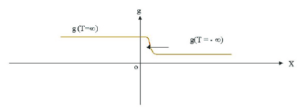
Figure 6. Necking of a 1D Rod

8.6. Example: Variation of Material Metric $g$ due to the Chemical Degradation

Here the evolution of the uniform material metric to the piecewise constant metric with the jump along the interface between a layer of chemically degraded material and the original material follows the kinetics of chemical degradation (see [29]).

Consider a thin-walled thermoplastic tubing employed for transport of chemically aggressive fluid. In time, the inner surface layer of material undergoes chemical degradation due to interaction with aggressive fluid flow.

Chemical degradation is manifested in an increase of the material density $\rho_{0}$, significant reduction in toughness (resistance to cracking) and a subtle change in yield strength, Young’s modulus and other thermo-mechanical properties.

Assuming the homogeneity of degraded layer we see that the original euclidian material reference metric in degraded ring evolves (see the mass conservation law (3.4)) which generates a jump on the interface with the outer layer of unchanged material. Continuity of normal stresses on the interface allows us to describe the final state of the system by elementary methods presented below.

Consider a thin ring (see Figure 7) which represent the 2D cross-section of the tubing. The wall thickness $t=R_{o}-R_{i}$ is small in comparison to the outer radius $R_{o}$: $t/R_{o}\ll 1$. $R_{d}$ in Fig ** stands for the radius of interface between the layer of degraded material and unchanged layer. The depth of degradation $t_{d}=R_{d}-R_{i}$ is relatively small: $t_{d}/t\ll 1$.

Select the polar coordinate system $(r,\theta)$. 2D material metrics of the initial ($g^{0}$) and degraded ($g^{\prime}$) states are

$$g^{0}=\left(\begin{smallmatrix}1&0\\ 0&r(0)^{2}\end{smallmatrix}\right),\ |g^{0}|=r^{2}(0);\ g^{\prime}=\left(\begin{smallmatrix}1+\epsilon&0\\ 0&r^{{}^{\prime}2}\end{smallmatrix}\right),\ |g^{\prime}|=(1+\epsilon)r^{{}^{\prime}2},$$

where $r^{\prime}=(1+\epsilon)r$ and $\epsilon$ is a small variation of scale in the radial direction.

Mass conservation law $\rho_{0}\sqrt{|g^{0}|}=\rho_{0}^{\prime}\sqrt{|g^{\prime}|}$ relates density variation $\rho^{\prime}_{0}=\rho_{0}+\Delta\rho_{0},\ \frac{\Delta\rho_{0}}{\rho_{0}}\sim 10^{-3}$ with the change in material metric

$$\frac{\rho_{0}}{\rho_{0}+\Delta\rho_{0}}=\sqrt{\frac{(1+\epsilon)r^{{}^{\prime}2}}{r(0)^{2}}}=(1+\epsilon)^{3/2}\Longrightarrow 1-\frac{\Delta\rho_{0}}{\rho_{0}}\approx 1+\frac{3}{2}\epsilon+O(\epsilon^{2}).$$ (8.7)

Therefore $\epsilon\approx-\frac{2}{3}\frac{\Delta\rho_{0}}{\rho_{0}}+O(\epsilon^{2}).$

Thus, the densification (i.e. $\Delta\rho_{0}>0$) leads to the shrinkage of the thin ring of degraded material. If we remove the constrains on shrinkage applied by the outer ring of original material the gap

$$w=R_{d}^{0}-(1-\frac{2}{3}\frac{\Delta\rho_{0}}{\rho_{0}})R^{0}_{d}=\frac{2}{3}\frac{\Delta\rho_{0}}{\rho_{0}}R^{0}_{d}$$ (8.8)

appears.

As a result of such constrains, the degraded material should be elastically stretched to close the gap $w$. This elastic deformation has the form

$$\phi(r,\theta)=\begin{cases}r^{\prime\prime}(r)=(1+\frac{2}{3}\frac{\Delta\rho_{0}}{\rho_{0}})r^{\prime},\\ \theta^{\prime\prime}=\theta^{\prime}=\theta.\end{cases}$$

Under such a deformation elastic strain tensor $E^{el}=\frac{1}{2}g^{-1}(C_{3}(\phi)-g),C_{3}(\phi)=h_{ij}\phi^{i}_{,I}\phi^{j}_{,J}$ has the form

$$E^{el}\approx\frac{2}{3}\frac{\Delta\rho_{0}}{\rho_{0}}\begin{pmatrix}1&0\\ 0&1\end{pmatrix}.$$ (8.9)

The tensile strain (8.9) is directly translated into the tensile radial stress via Hooke’s law

$$\sigma_{rr}=\frac{Y}{1-\nu}\frac{2}{3}\frac{\Delta\rho_{0}}{\rho_{0}}.$$

Although hoop stresses $\sigma_{r\theta}$ may be discontinuous, the equilibrium conditions requires continuity of radial stress across the interface, ,

$$\sigma_{rr}n_{r}|_{r=R_{d}-0}=\sigma_{rr}n_{r}|_{r=R_{d}+0}.$$

This implies that the outer ring of original material experiences compressive stresses while the inner degraded layer is under tension. The elastic strains $E^{el}$ jointly close the gap $w$ and restore the compatibility of the Cauchy metric $g_{final}$ in the whole domain:

$$g_{final}=g^{\prime}+E^{el}.$$

Therefore while the material metric $g^{\prime}$ has the jump leading to the nonzero singular curvature along the interface, the final metric is continuous and flat.

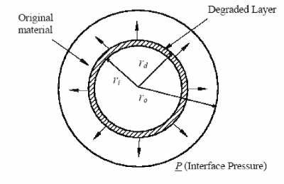
Figure 7. A sketch of polymer tubing cross section with inner degraded layer

9. Physical and Material Balance Laws

As it is typical for a Lagrangian Field Theory, action of any one-parameter group of transformations of the space $P\times M$, commuting with the projection to $P$, leads to the corresponding balance law (See [6]). In particular, translations in the ”physical” space-time $M$ lead to the dynamical equations (7.1-2), rotations in $M$ lead to the angular momentum balance law (conservation law in the absence of applied torque). Respectively, translations in the ”material space-time” $P$ lead to the energy balance law (translations along the time $T$ axis) and to the material momentum balance law (”pseudomomentum” balance, ([20], [30], [31]), rotations in the material space $B$ lead to the ”material angular momentum” balance law ([20]).

In the table below we present basic balance laws together with the transformations generating them. It is instructive to compare the space and material balance laws as it has been considered previously by several authors ([30], [31]).

Table 1. Space and Material Balance Laws

Symmetry	Physical space-time (Material independent)	Material space-time (Space independent)
Homogeneity of 3D-space	Linear momentum balance law (Equilibrium equations) $div(\sigma)=f$	Material momentum (pseudo- (-momentum) balance law div(b)=fmat
Time homogeneity	Energy balance law: $\partial_{t}{\mathcal{E}}^{tot}=div({\mathcal{P}}^{tot}$ )	Energy balance law
Isotropy of 3D-space	Angular momentum balance law $\equiv$ h-symmetry of Cauchy stress tensor $\sigma$: $\ \ \ \mathbf{I:\sigma=\sigma:I}$	Material angular momentum balance law $\equiv$ $C$-symmetry of Eshelby stress tensor b $\mathbf{b:C=C:b}$

Space and Material balance (conservation) laws are related via the deformation gradient $d\phi$. Restricting ourselves to the synchronized case and writing the material balance laws in the form $\eta_{I}=0$ and their ”physical” counterparts in the form $\nu_{i}=0$ we get the relationsship between these families of balance laws

$$\left(\begin{array}[]{c}\eta_{0}\\ \ldots\\ \ \eta_{4}\end{array}\right)=\left(\begin{array}[]{cccc}1&\phi^{1}_{,0}&\ldots&\phi^{3}_{,0}\\ 1&\phi^{1}_{,1}&\ldots&\phi^{3}_{,1}\\ \ldots&\ldots&\ldots&\ldots\\ 0&\ldots&\ldots&\phi^{3}_{,3}\end{array}\right)\cdot\left(\begin{array}[]{c}\nu_{0}\\ \ldots\\ \nu_{4}\end{array}\right)$$ (9.1)

Similar to the case of relativistic elasticity ([8]), the system of material balance laws $\eta_{I}=0,\ I=1,2,3$ is equivalent to the elasticity equations $\nu_{i}=0,\ i=1,2,3$, while the energy balance law $\eta_{0}=0$ (which here is the material conservation law as well as the physical one: in the case of synchronized history of deformation $\phi$ material time $T$ and physical time $t$ coincide). As a result, the energy conservation law is the consequence of the time translation invariance in both senses and follows from any of these two systems: $\eta_{0}=\sum_{i=1}^{i=3}\phi^{i}_{,0}\nu_{i}.$ This reflects the fact that the deformation we consider here are not truly 4-dimensional.

Balance laws (with the source terms) can be transformed into conservation laws by adding new dynamical variables. In the theory of uniform materials ([20, 24, 32]) it is zero curvature connection in the frame bundle over $M$ that is added to the list of conventional dynamical variables, in our scheme - it is the 4D material metric $G$.

10. Energy-Momentum Balance Law and the Eshelby Tensor.

In this section we consider the Energy-Momentum balance law resulting from the Least Action Principle and the space-time symmetries.

Consider local rigid translations in the material space-time $X^{J}\longmapsto X^{J}+\delta X^{J}.$ They generate a variation of components $\phi^{i}$ of the deformations, components $G_{IJ}$ of material metric and their derivatives (we follow the arguments of J.Eshelby ([21]).

Taking the variation of the Lagrangian density ${\mathcal{L}}=\sqrt{|G|}L=\sqrt{|G|}(L_{g}(G)+L_{e}(G,E^{el}))$ with respect to the material coordinates $X^{J}$, one obtains

$$\frac{\delta{\mathcal{L}}}{\delta X^{J}} = \sum_{i=0}^{i=3}\frac{\delta{\mathcal{L}}}{\delta\phi^{i}}\phi^{i}_{,J}+\frac{\partial}{\partial X^{I}}(\sum_{i=1}^{i=3}\frac{\partial{\mathcal{L}}}{\partial\phi^{i}_{,I}}\phi^{i}_{,J})+\frac{\delta{\mathcal{L}}}{\delta G^{AB}}G^{AB}_{,J}+$$ (10.1)

$$\frac{\partial}{\partial X^{I}}\left({\mathcal{E}}(G)^{I}_{J}=\frac{\partial{\mathcal{L}}}{\partial G^{AB}_{,I}}G^{AB}_{,J}+\frac{\partial{\mathcal{L}}}{\partial G^{AB}_{,IK}}G^{AB}_{,KJ}-\frac{\partial}{\partial X^{K}}\left(\frac{\partial{\mathcal{L}}}{\partial G^{AB}_{,IK}}\right)G^{AB}_{,J}\right).\hskip 22.76228pt$$

The last term in the right side of (10.1) includes a definition of the (1,1)-tensor density ${\mathcal{E}}(G)$. Employing the Euler-Lagrange equations (7.1-2), we obtain for the Total Energy-Momentum Tensor (density)

$${\mathcal{E}}^{tot}=-{\mathcal{L}}\delta^{I}_{J}-S^{I}_{J}+{\mathcal{E}}(G)^{I}_{J},$$ (10.2)

the conservation law

$$div_{G_{0}}({\mathcal{E}}^{tot})=\frac{\partial}{\partial X^{I}}{\mathcal{E}}^{tot\ I}_{J}=0,\ J=0,1,2,3.$$ (10.3)

Divergence here is taken with respect to the 4D ”reference” metric $G_{0}$. Since $L_{m}$ does not depend on deformation $\phi$ and the body forces potential $U$ does not depend on its derivatives while $L_{e}=-\rho_{0}f-\rho_{0}U$,

$${\mathcal{S}}^{I}_{J}=-\sum_{i=1}^{i=3}\frac{\partial{\mathcal{L}}}{\partial\phi^{i}_{,I}}\phi^{i}_{,J}=\sum_{i=1}^{i=3}P^{I}_{i}\phi^{i}_{J}S\sqrt{|g|},$$ (10.4)

which is the 4D-version of the (density of) Second Piola-Kirchoff Stress Tensor.

Rewrite ${\mathcal{E}}^{tot}$ in the form: ${\mathcal{E}}^{tot}={\mathcal{B}}+U\delta^{I}_{J}\sqrt{\|G\|}+{\mathcal{L}}_{m}\delta^{I}_{J}+{\mathcal{E}}(G)$ where we denoted by $\mathcal{B}$ the tensor density ${\mathcal{B}}=b\sqrt{|G|}$ of the Eshelby EM Tensor. Then the equation (10.3) takes the form

$$div_{G_{0}}{\mathcal{B}}={\mathcal{B}}^{I}_{J,I}=-div_{G_{0}}(U\delta^{I}_{J}\sqrt{\|G\|}+{\mathcal{L}}_{m}\delta^{I}_{J}+{\mathcal{E}}(G)),$$ (10.5)

where in the right side only metrical quantities and the potential $U$ of the body forces are left.

The second term and the metrical part of the third term in the right side of (10.5) are related to the ground state of the Lagrangian density i.e. to the inhomogeneity of ”cohesive energy” and the ”material flows”. The elastic part of the third term on the right is related to a variation of elastic moduli if these moduli depend on the derivatives of the metric $G$. Equality (10.5) can be easily rewritten in terms of covariant derivatives with respect to the metric $G$.

Taking $J=0$ in (10.6) we arrive at the energy conservation law in ADM notations (using $t$ instead of $X^{0}$)

$$\frac{\partial}{\partial t}((f+U+L_{m})S\sqrt{|g|}+{\mathcal{E}}^{0}_{0})=\sum_{I=1}^{I=3}\frac{\partial}{\partial X^{I}}\left(\sum_{i=1}^{i=3}P^{I}_{i}\phi^{i}_{,0}S\sqrt{|g|}-{\mathcal{E}}(G)^{I}_{0}.\right)$$ (10.6)

Equation (10.6) has the form $\frac{\partial({\mbox{T}otalEnergyDensity})}{\partial T}={\mbox{T}otalFlowDensity},$ with the total (inner) energy density given by

$${\mathcal{E}}^{tot\ 0}_{0}=(f+U+L_{m})S\sqrt{|g|}+{\mathcal{E}}(G)^{0}_{0}.$$ (10.7)

The total energy is the sum of the following parts: elastic energy $f$, potential energy of the volume forces $U$ , cohesive ”ground state” energy - the term $F(E^{in},S)$ in $L_{m}$, inhomogeneities energy from the curvature density $\beta R(g)S\sqrt{|g|}$ and corresponding terms of ${\mathcal{E}}^{0}_{0}$, ”kinetic metric energy” that is defined by the term s produced by $\chi(K)$ in $L_{m}$ and ${\mathcal{E}}^{0}_{0}$ and reflects the intensity of irreversible deformation and ”metrical volume change energy” coming from the $div_{g}({\vec{N}})$-terms.

The sum on the right side of (10.5) consists of the flow of the Piola-Kirchoff stress tensor density $\sum_{I=1}^{I=3}[P^{I}_{i}\phi^{i}_{,0}S\sqrt{|g|}]_{,I}$ and the flows related to the change of the material metric - internal material flows, flows of inhomogeneities (coming from the curvature $R(g)$ etc.

If the metric $G$ does not depend on time (i.e. ${\bar{N}}=0,K=0,\ G=G_{0}$) and if $Ric(g_{t})=0$, one obtains the conventional energy conservation law of Elasticity Theory ([6], Chapter 5, Sec.5): $\frac{\partial(f+U)}{\partial T}=-\sum_{I=1}^{I=3}\frac{\partial}{\partial X^{I}}(P^{I}_{i}\phi^{i}_{,0}),$.

Example 2 (Block diagonal metric $G$, synchronous deformation and homogeneous media).

In this case we have $Ric(g_{t})=0,\ {\tilde{N}}=0,g=g(t),S=S(t)$, the extrinsic curvature has the form $K^{I}_{J}=\left(\begin{array}[]{cc}0&0\\ 0&S^{-1}g^{IK}g_{KJ,0}\end{array}\right)$ and $\chi(K)$ is the only term in the Lagrangian containing time derivatives.

In addition to this, no flow terms except the usual Piola-Kirchoff flow appear on the right side in the energy balance law which takes the form

$$\frac{\partial}{\partial t}\left((f+U+L_{m})S\sqrt{|g|}+S^{-1}g_{AB,0}\left[\frac{\partial\chi}{K^{M}_{B}}g^{MA}+\frac{\partial\chi}{K^{M}_{A}}g^{MB}\right]S\sqrt{|g|}\right)=+\sum_{I=1}^{I=3}(P^{I}_{i}\phi^{i}_{,0}S\sqrt{|g|})_{,I}.$$ (10.8)

This equation describes how the energy supplied by the boundary load spreads not just to the increase of the strain energy, but also to the change of its ”cohesive energy” of the material ($F(S,|g|)$) and to the acceleration of the aging processes.

11. Aging of a homogeneous rod

In considering three types of inelastic processes in a tensile homogeneous rod: unconstrained aging, stress relaxation and creep (see [19] for more detailed exposition) we assume that ${\vec{N}}=0,R(g)=0$, $S(t=0)=1$ and that $S(t)$ is increasing to a certain level depending on the initial state of the body and the process.

11.1. Deformation, strain tensors and tensor $K$

Introduce material cylindrical coordinates $(R,\Theta,Z)$ in the reference state of a rod $B$. Spacial cylindrical coordinates $(r,\theta,z)$ are introduced in the physical space $R^{3}$. In addition we normalize the initial state $g(0)$ of material metric taking $g(0)=g_{0}$.

We consider the class of time dependent (total) deformations $\phi$ of the from

$$\phi_{t}:(R,\Theta,Z)\rightarrow(r=\mu(t,Z)R,\theta=\Theta,Z=k(Z,t)),$$ (11.1)

with $\mu,k$ representing amount of ”stretch” in radial and axial directions respectively.

Material metric $g_{t}$ is flat (homogeneous case!) and is generated by a global deformation $\phi_{m}$ of the same type as (11.1), with $\mu_{m},k_{m}$ the same as above: $g_{t}=\phi_{m}(t,\cdot)^{*}h$. As a result

$$g=\phi_{m}^{*}h=\left(\begin{smallmatrix}\mu_{m}^{2}&0&R\mu_{m}\mu_{m,Z}\\ 0&R^{2}\mu^{2}_{m}&0\\ R\mu_{m}\mu_{m,Z}&0&\lambda^{2}+R^{2}\mu^{2}_{m,Z}\end{smallmatrix}\right),\ C(\phi)=\left(\begin{smallmatrix}{\mu}^{2}&0&R{\mu}{\mu}_{,Z}\\ 0&R^{2}{\mu}^{2}&0\\ R{\mu}{\mu}_{,Z}&0&\lambda^{2}+R^{2}{\mu}^{2}_{,Z}\end{smallmatrix}\right),$$ (11.2)

where $\lambda=k_{,Z},\lambda_{m}=k_{m,Z}$. For a homogeneous rod $k(Z,t)=\lambda(t)Z,\ k_{m}(Z,t)=\lambda_{m}(t)Z$.

In the elasticity theory (see [33]) it is customary to present deformation (total and inelastic as well) as the composition of a uniform dilatation with the axial expansion factor $\lambda_{v}(t)$ and of the volume preserving normal expansion with the factor $\lambda_{d}$: $\lambda=\lambda_{v}\lambda_{d}$. We will obtain $\mu=\lambda_{v}\lambda_{d}^{-1/2}$ and $\sqrt{|g|}=\lambda_{v}^{3}R$ (and the same for $\lambda_{mv},\lambda_{md}$).

As a result, the inelastic strain tensor can be written in the following form

$$E^{in}=\frac{1}{2}(g_{0}^{-1}g)=\left(\begin{smallmatrix}ln(\mu)&0&0\\ 0&ln(\mu)&0\\ 0&0&ln(\lambda)\end{smallmatrix}\right)=\left(\begin{smallmatrix}\xi-\frac{1}{2}\eta&0&0\\ 0&\xi-\frac{1}{2}\eta&0\\ 0&0&\xi+\eta\end{smallmatrix}\right)$$ (11.3)

Here we introduced the variables $\xi=ln(\lambda_{m\ v}),\eta=ln(\lambda_{m\ d})$. As a result, calculating basic invariants of these tensors we see that the ”ground state” energy $F$ is the function of $S,\xi,\eta^{2}.$

Decomposing the total deformation as the composition of inelastic and elastic one and assuming that elastic deformation is small compared to $1$ we write:

$$\lambda_{v}=\lambda_{v\ m}(1+\epsilon_{v}),\ \lambda_{d}=\lambda_{d\ m}(1+\epsilon_{d}).$$

In these notations elastic strain tensor takes the conventional diagonal form

$$E^{el}=\frac{1}{2}ln(g^{-1}C({\phi^{tot}}))\approx diag(\ \epsilon_{v}-\frac{1}{2}\epsilon_{d},\epsilon_{v}-\frac{1}{2}\epsilon_{d},\epsilon_{v}+\epsilon_{d}).$$

Strain energy for our (homogeneous) rod will now take the form

$$f=\frac{K}{2}\epsilon_{v}^{2}+\frac{3\mu}{2}\epsilon_{d}^{2}$$ (11.4)

with the bulk coefficient $K$ and the Lame coefficient $\mu$.

Mass conservation law (3.4) takes the form $\rho_{0}(t)=\lambda_{v}^{3}\rho_{0}(0).$

The spacial part of the tensor $K$ for a homogeneous rod takes the diagonal form

$$K=S^{-1}diag(2\xi_{t}-\eta_{t},2\xi_{t}+2\eta_{t},2\xi_{t}-\eta_{t}).$$ (11.5)

Thus, $Tr(K)=6S^{-1}\xi_{t},\ Tr(K-\frac{1}{3}Tr(K)I)^{2}=6S^{-2}\eta_{t}^{2}$ and dissipative potential $\chi(K)$ is the function of arguments $S^{-1}\xi_{t},S^{-1}\eta_{t}$.

Remark 4.

In general, aging equation for the described situation have the form of a 3D degenerate Lagrangian system (we refer to [19], or [34] for more details). In the cases of the processes studied below this system reduces to the 2D degenerate dynamical system. In all three cases one can trivially solve elasticity equations, exclude elastic variables $\epsilon_{v},\epsilon_{d}$ from aging equations and, therefore, to close the system of aging equations.

11.2. Unconstrained aging.

Unconstrained aging (shortly UA) is the simplest example of a material evolution. A sample of material (rod) is prepared and then is left without any constraints or load applied to it. Usually the process of aging is manifested in a variation of material density, or a specific volume change up to a saturation point, when the observable evolution stops. In many polymers the aging is accompanied by shrinkage up to a few percent of initial volume. This diminishing in volume (2-5%) is called unconstrained aging. We discuss here a model for UA in terms of variables $(S,\xi)$ (dilatational deformation plays negligible role in UA). No strain energy is present, stress is zero.

We take the ”ground state energy” to be

$$F_{UA}(S,\xi)=(c_{1}+c_{2}S+(p\xi S^{-1}+k\xi^{2})$$

with $k>0,p<0,c_{1}<0,c_{2}>0$ and the dissipative potential

$$\chi_{UA}(K)=\alpha(S^{-1}\xi_{t})^{2}.$$

Integrating over the volume of the rod we get the action in the form

$$A(\xi,S)=V\int_{0}^{T}((c_{1}S+c_{2}S^{2}+(p\xi+k\xi^{2}S)+\alpha S(S^{-1}\xi_{t})^{2})dt.$$ (11.6)

Euler-Lagrange Equations of UA can be reduced to the following dynamical system

$$\begin{cases}\xi_{t}&=-S\left(\frac{c_{1}+2c_{2}S+k\xi^{2}}{\alpha}\right)^{\frac{1}{2}},\\ S_{t}&=-\frac{p}{2c_{2}}\left(\frac{c_{1}+2c_{2}S+k\xi^{2}}{\alpha}\right)^{\frac{1}{2}}.\end{cases}$$ (11.7)

We have here $\xi_{t}\leqq 0,S_{t}\geqq 0$.

Equation (7.5) takes here the form $\alpha\xi_{t}^{2}=S^{2}\frac{\partial(\tilde{F})}{\partial S},$ where $\tilde{F}=SF$.

Take $\alpha=-1$. Then, the domain of admissible dynamics defined by the positivity of expression under the square root is

$$S\leqq-\frac{1}{2c_{2}}(c_{1}+k\xi^{2}),$$ (11.8)

and the curve where evolution stops when the phase trajectory reaches the final state is $S=-\frac{1}{2c_{2}}(c_{1}+k\xi^{2}).$

The ”ground state energy” $F$ is negative at initial moment and that it increases during the evolution.

System (11.7) has the first integral $J=c_{2}S^{2}-p\xi.$ Choosing an initial point $(S(0),\xi(0)=0)$ of a trajectory $\Gamma$ in the domain of admissible dynamics. Along $\Gamma$ we have $J(\xi,S)=J(S(0),0)$ If we calculate $S(t)$ as the function of $\xi(t)$ along $\Gamma$, substitute into the first equation (11.7) and separate variables in this equation we get the $\xi(t)$ as the explicit function of parameters of the problem and initial value $S(0)$ in terms of elliptic functions (see [19]).

Figure 8 shows a family of shrinkage curves corresponding to the various values of $S(0)=1,1.3,1.6,1.9$ (which represent the initial aging of the material). Apparently, the higher is the initial age, the less shrinkage is observed.

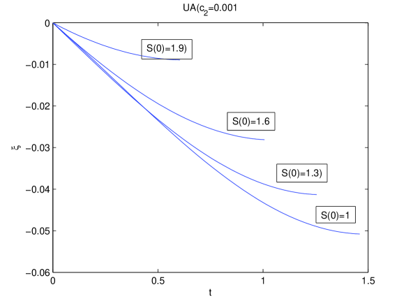
Figure 8. Aging curves

When a load applied to the rod reaches certain level, new processes may start. These new processes (going on the background of the UA) initiate action of a new part of the ”ground state” $F(S,\xi,\eta)$ and activates the new kinetic potential $\chi_{2}(K)$. For the description of stress relaxation and creep we choose the dissipative potential $\chi_{2}(K)=\frac{K}{\beta D}ln(\frac{K}{D})-\frac{1}{\beta}(1+\frac{K}{D})ln(1+\frac{K}{D})$ corresponding to the phenomenological Dorn relation between the stress and the strain rate $\dot{\eta}$ (see [36], Sec.2.3 and the footnote in Sec.5 above). Unconstrained aging is much slower and leads to smaller changes then both stress relaxation and the creep. That is why we may with good accuracy disregard the UA while describing two other processes.

11.3. Stress relaxation

In the case of a stress relaxation (SR) we fix the rod of initial length $L$ at the left end and then quickly pull (or compress) it uniaxially and fast (elastically) until it reach certain length $L^{*}.$ Then we fix right end as well, leaving side surface of the rod free. In this configuration the only component of Cauchy stress that is nonzero is $\sigma_{zz}$. For the SR the volume change is negligible and we have $\lambda_{m\ v}=1,\lambda_{m}=\lambda_{m\ d}$

Initially all the stretching is due to elastic process and $\lambda^{*}_{d}=L^{*}/L=(1+\epsilon_{z}(0)).$ Then the inelastic deformation starts to increase in expense of elastic one maintaining the total strain constant. The reduction of elastic strain is directly translated into the reduction of stresses via Hooke’s law. The total elongation at moment $t$ can be decomposed as follows

$$\lambda^{*}_{d}=(1+\epsilon_{z}(t))\lambda_{m,d}(t)=(1+\epsilon_{z}(t))e^{\eta(t)}$$ (11.9)

and therefore $\epsilon_{z}(t)=\eta^{*}-\eta(t),$ where $\eta^{*}=ln(\lambda^{*}).$

From Hooke’s law $\sigma_{zz}=Y\epsilon_{z},$ where $Y$ is the Young module. Thus for the strain energy expression we obtain

$$f(\eta)=\frac{1}{2}\sigma_{zz}\epsilon_{z}=\frac{1}{2}Y\epsilon_{z}^{2}=\frac{Y}{2}(\eta^{*}-\eta(t))^{2}.$$ (11.10)

For pure stress relaxation (without background UA)

$$F=F_{SR}(S,\eta)=(q_{1}+q_{2}S)+\eta(b_{0}S^{-1}+b_{1}+a_{1}\eta),\ q_{1}<0,q_{2}<0,b_{0}<0,a_{1}<0,$$

with the coefficients different from those of the slow UA.

Action $A(S(t),\eta(t))$ now takes the form

$$A(S,\eta)=\int_{0}^{T}\left[(q_{1}+q_{2}S)+\eta(b_{0}S^{-1}+b_{1}+a_{1}\eta)+\frac{Y}{2}(\eta^{*}-\eta(t))^{2}+S\chi(S^{-1}\eta_{t})\right]Sdt=\\ =\int_{0}^{T}\left[{\tilde{F}}_{SR}(S,\eta)+S\chi(S^{-1}\eta_{t})\right]dt,$$ (11.11)

where

$${\tilde{F}}_{SR}(S,\eta)=SF_{SR}=(q_{1}S+q_{2}S^{2})+\eta(b_{0}+b_{1}S+a_{1}\eta S)+S\frac{Y}{2}(\eta^{*}-\eta(t))^{2}=\\ q_{2}S^{2}+p_{2}(\eta)S,$$ (11.12)

where $p_{2}(\eta)=(q_{1}+\frac{Y}{2}\eta^{*\ 2})+(b_{1}-Y\eta^{*})\eta+(a_{1}+\frac{Y}{2})\eta^{2}.$

We have ${\tilde{F}}_{S}=2q_{2}S+p_{2}(\eta)$ and the domain of admissible motion is defined by

$$D_{ad}=\{(\eta,S)|\eta>0,S\geqq 1,\ S<-\frac{p_{2}(\eta)}{2q_{2}}\},$$

while the stoping curve has the form $S=-\frac{p_{2}(\eta)}{2q_{2}}.$

Aging equations (7.5-7.7) will now take the form

$$\begin{cases}\eta_{t}&=S\psi^{-1}(2q_{2}S+p_{2}(\eta))=S\psi^{-1}(2q_{2}S+[(q_{1}+\frac{Y}{2}\eta^{*\ 2})+(b_{1}-Y\eta^{*})\eta+(a_{1}+\frac{Y}{2})\eta^{2}]),\\ S_{t}&=\frac{b_{0}}{2q_{2}}\psi^{-1}(2q_{2}S+p_{2}(\eta))=S\psi^{-1}(2q_{2}S+[(q_{1}+\frac{Y}{2}\eta^{*\ 2})+(b_{1}-Y\eta^{*})\eta+(a_{1}+\frac{Y}{2})\eta^{2}]).\end{cases}$$ (11.13)

This system has the first integral $J=b_{0}\eta-q_{2}S^{2},$ and the phase trajectory corresponding to the initial value $S=S(0),\eta(0)=0$ has the form $S=\sqrt{S(0)^{2}+\frac{b_{0}}{q_{2}}\eta}.$ Using this one can find analytic solutions $\eta(t)$ in terms of elliptic functions ([19]).

On the Figure 9 we present results of calculations of the stress relaxation $\sigma_{zz}(t)$ for several values of initial stretching $L=0.1,0.15,0.2,0.5$ and for realistic values of parameters of the problem. Values of $\sigma_{zz}(t)$ are found by solving numerically system (11.13) for $\eta(t)$, calculating elastic strain $\epsilon_{z}(t)$ and using the Hooke’s law. Apparently, the higher is the value of initial stretching, the sharper is the stress relaxation curve and the higher is the asymptotic value of stress.

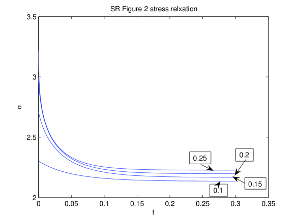
Figure 9. Stress Relaxation: Stress $\sigma_{zz}(t).$ for $\eta^{*}=0.1,0.15,0.2,0.25$.

11.4. Creep

In the case of the creep we fix the left end of the rod and apply force $\mathcal{F}$ in $Z$-direction to its right end. If this force is large enough (i.e. if the concentration of elastic energy $f$ in the rod is larger then an activation threshold), the creep starts - inelastic deformation that goes on for some time until the rod brakes. Thus, at the moment when the inelastic strain $\eta(t)$ starts growing from zero, there should be a supply of strain energy obtained from the work of the stress $\sigma_{zz}=\frac{\mathcal{F}}{A(t)}$ on elastic deformation. Denote by $f_{in}$ this strain energy (of initiation).

During the creep the homogeneous component $\sigma_{zz}$ of stress is equal

$$\sigma_{zz}(t)=\frac{{\mathcal{F}}}{A(t)}=\frac{{\mathcal{F}}}{\lambda_{v}(t)^{2}\lambda_{d}^{-1}(t)A_{0}}=\frac{\lambda_{d}(t){\mathcal{F}}}{A_{0}}=\frac{e^{\eta}{\mathcal{F}}}{A_{0}}.$$ (11.14)

The last equality is true given the assumption (natural for a conventional creep) that inelastic volume change is negligible, i.e. $\lambda_{v}=1,\ \xi=0$., for a constant force $\mathcal{F}$ and variable cross-section area $A(t)$.

Using the Hooke’s law one can show that $\epsilon_{z}=\frac{\sigma_{zz}}{Y}$ and that the strain energy is equal to $f=\frac{{\mathcal{F}}^{2}e^{2\eta}}{2YA(0)^{2}}$.

Calculating the work of the load $\mathcal{F}$ on the total way $L(e^{\eta(t)}-1)$ of the right end of the rod we get the additional term in the Lagrangian (work of load on the inelastic deformation) equal $\frac{\mathcal{F}}{A_{0}}(e^{\eta}-1)$.

Overall action takes the form ($\xi(t)=0$)

$${\mathcal{L}}(S(t),\eta(t))=[F_{CR}(S,\eta)+\frac{\mathcal{F}}{A_{0}}(e^{\eta}-1)+\phi(S^{-1}\eta_{t})+\Lambda{\mathcal{F}}^{2}e^{2\eta}]Sdt,$$ (11.15)

where $F(S,\eta)$ is the same as for stress relaxation.

Acting as before we get the following dynamical system for parameters $\eta,S$:

$$\begin{cases}\eta_{t}&=S\psi^{-1}(\frac{\mathcal{F}}{A_{0}}(e^{\eta}-1)+\Lambda{\mathcal{F}}^{2}e^{2\eta}+(q_{1}+2q_{2}S+b_{1}\eta+a_{1}\eta^{2})),\\ S_{t}&=\frac{b_{0}}{2q_{2}}\psi^{-1}(\frac{\mathcal{F}}{A_{0}}(e^{\eta}-1)+\Lambda{\mathcal{F}}^{2}e^{2\eta}+(q_{1}+2q_{2}S+b_{1}\eta+a_{1}\eta^{2})).\end{cases}$$ (11.16)

where $\psi(x)=(e^{Dx}-1)_{+}$ function as in the case of stress relaxation. We have in this system $\eta_{t}\geqq 0,S_{t}\geqq 0$ for the admissible initial values $S(0),\eta(0)$.

For the creep to start, the argument of the function $\psi(x)$ in the system should be positive at initial moment. Since $\sigma_{zz}=\frac{{\mathcal{F}}e^{\eta}}{A_{0}}$, this condition takes the form

$$\frac{\sigma(0)^{2}}{2Y}+q_{1}+2q_{2}S(0)+a_{1}\eta(0)^{2}>0.$$ (11.17)

Since $q_{1},q_{2},a_{1}$ are negative parameters, the inequality (11.17) defines the stress (or strain energy - $f_{in}$) threshold for the initiation of the creep processes (see [35], p.7).

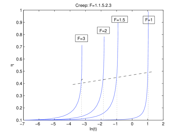
Figure 10. Creep: inelastic strain $\eta(t)$ for $F=1,1.5,2$ and 3.

On the Figure 11 the graphs of $\eta(t)$ for the creep are presented for different values of the force $\frac{F}{A_{0}}=1,1.5,2$ ($A_{0}=1$). There is a point on each trajectory, corresponding to the instability of creep deformation where the cross-section of the rod diminishes to zero and the rod fails in so called ductile manner. As it can be seen from the results of calculations, the higher is the force, the faster creep deformation develops and the time to the ductile failure becomes significantly shorter, for example, three times increase in force results in more then 3 order of magnitude in time to failure.

Comparing these graphs with the experimental data ([35, 36]) we see the good qualitative (and, for some materials, quantitative) agreement.

12. Appendix A. Strain energy as a perturbation of the ”ground state energy”.

In this section we discuss perturbation scheme of a ground state Lagrangian $F(E^{in},S,{\bar{N}}),\ E^{in}=\frac{1}{2}\ln(g_{0}^{-1}g)$ by elastic deformation, assuming that elastic strain tensor is small in compare to the inelastic one.

In the pure inelastic mode of behavior (free aging, special load that produces $C(\phi)=g$) only metric quantities $g,S,{\bar{N}}$ enter the total Lagrangian $L$. Under the general load the material metric $g$ is deformed into $C(\phi)$ and total deformation $E^{tot}=\frac{1}{2}\ln(g_{0}^{-1}C(\phi))$ takes the place of $E^{in}$.

Assuming that $g^{-1}C(\phi)\approx I+small$, so that $E^{el}\ll E^{in}$ we decompose $g^{-1}_{0}C(\phi)=(g^{-1}_{0}g)\cdot(g^{-1}C(\phi)).$ Taking logarithm, we obtain

$$E^{tot}=\frac{1}{2}\ln(exp(2E^{in})\cdot exp(2E^{el}))\simeq\frac{1}{2}\ln(exp(2E^{in})\cdot(I+2E^{el}))$$

Here we’ve used the linear approximation $exp(2E^{el})\simeq I+2E^{el}$. Using the Campbell- Hausdorff-Dynkin formula we get

$$E^{tot}\simeq\frac{1}{2}[\ln(exp(2E^{in}))+Ad(exp(2E^{in}))2E^{el}]=E^{in}+Ad(exp(2E^{in}))E^{el}.$$ (12.1)

We consider the ”total ground state” Lagrangian $F$ depending on $E^{tot}$ through its invariants $I_{k}(E^{tot}),\ k=1,2,3$. Then we decompose it into Taylor series by considering $E^{el}$ small in compare to $E^{in}$. The approximate expression for $E^{tot}$ above gives us up to the second order terms

$$I_{k}(E^{tot})\simeq I_{k}(E^{in})+dI_{k}(E^{in})(E^{el\ g_{0}^{-1}g})+d^{2}I_{k}(E^{in})(E^{el\ g_{0}^{-1}g},E^{el\ g_{0}^{-1}g})+h.o.t..$$ (12.2)

Substituting this into the metric term $F(I_{k}(E^{tot})$ (for this discussion we suppress in $F$ all other arguments it depends on) we get, after recombining its terms, its decomposition up to the second order

$$F(E^{tot})\simeq F(E^{in})+\sum_{k}F_{,I_{k}}(E^{in})<dI_{k}(E^{in}),E^{el\ g_{0}^{-1}g}>+\\ +\{\sum_{k}F_{,I_{k}}(E^{in})<d^{2}I_{k}(E^{in})(E^{el\ g_{0}^{-1}g},E^{el\ g_{0}^{-1}g})+\\ +\sum_{ij}F_{I_{i}I_{j}}(E^{in})<dI_{i}(E^{in}),E^{el\ g_{0}^{-1}g}><dI_{j}(E^{in}),E^{el\ g_{0}^{-1}g}>\}$$ (12.3)

In this formula first term on the right is the basic metric (”ground state”) energy describing, in particular, equilibrium values for the metric $g$ (see example below).

The second term, linear by $E^{el}$ describes the interaction of elastic and inelastic processes. In the absence of such interactions or other material processes $g$ takes the value delivering minimum to the basic energy $F(E^{in})$. Therefore, its differential takes a zero value for corresponding value of the argument $E^{in}$ and linear term vanishes.

Finally, the quadratic form in formula (12.3) is the conventional elastic (strain) energy with variable and possible inhomogeneous elasticity tensor.

During the active processes of configurational changes in the material (aging, in the zone of phase transition) this elasticity tensor as well as the basic energy plays an active role in the evolution. But when such processes stops (no aging happens or wave of phase transition passed) and the material metric $g$ is locked in some stable state (local minimum of $F$?), the value of this tensor is also locked at the corresponding value (see below).

In order to calculate the elasticity tensor $e$ we have to calculate differentials of invariants $I_{k}$ of the inelastic strain tensor $E^{in}$. We choose momenta $Tr(E^{k})$ as the basic invariants of a (1,1)-tensors ([32]). In our, 3D case we have $I_{1}(E)=Tr(E),I_{2}(E)=Tr(E^{2}),I_{3}(E)=det(E).$ Thus, we have for its first differentials ([32])

$$\frac{\partial I_{1}(E)}{E^{I}_{J}}=\delta^{J}_{I};\ \frac{\partial I_{2}(E)}{E^{I}_{J}}=2E^{J}_{I};\ \frac{\partial I_{3}(E)}{E^{I}_{J}}=3E^{J}_{K}E^{K}_{I}=3E^{2\ J}_{I}.$$

and $<dI_{1}(E),P>=Tr(P);\ <dI_{2}(E),P>=2Tr(EP);\ <dI_{3}(E),P>=3Tr(E^{2}P).$ Here we are using multiplication of (1,1)-tensors. The second differentials of momenta have the form $d^{2}I_{1}(E)=0;\ d^{2}I_{2}(E)(B,B)=2Tr(B^{2});\ d^{2}I_{3}(E)(B,B)=6Tr(EB^{2}).$

Before using these expressions for differentials we notice that since $g_{0}^{-1}g=exp(2E^{in})$, $(E^{in})^{g_{0}^{-1}g}=E^{in}$ and due to the properties of $Tr$ for all natural powers $a,b$ one has $Tr(E^{in\ a}((E^{el})^{g_{0}^{-1}g\ })^{b})=Tr(E^{in\ a}E^{el\ b}).$ Thus, conjugation by $g_{0}^{-1}g$ disappear from the formulas for Elastic energy.

Substituting expression for differentials in (12.3) we get expression for $F(E^{tot})$ as the sum of ”constant”, linear by $E^{el}$ and quadratic by $E^{el}$ terms

$$F(E^{tot})\simeq F(E^{in})+Tr(CE^{el})+Tr({\mathbf{e}}:E^{el}:E^{el})$$ (12.4)

Here $C$ is the (1,1)-tensor

$$C=F_{,I_{1}}(E^{in})I+2F_{,I_{2}}(E^{in})E^{in}+3F_{,I_{3}}(E^{in})(E^{in})^{2},$$ (12.5)

and $\mathbf{e}$ the elasticity tensor

$${\mathbf{e}}^{BD}_{AC}=2F_{,I_{2}}(E^{in})\delta^{B}_{C}\delta^{D}_{A}+6F_{,I_{3}}(E^{in})^{B}_{C}\delta^{D}_{A}+2F_{,I_{1}I_{1}}(E^{in})\delta^{B}_{A}\delta^{D}_{C}+4F_{,I_{2}I_{2}}(E^{in})^{B}_{A}(E^{in})^{D}_{C}+\\ 9F_{,I_{3}I_{3}}(E^{in})^{2\ B}_{A}(E^{in})^{2\ D}_{C}+4F_{,I_{1}I_{2}}\delta^{B}_{A}(E^{in})^{D}_{C}+6F_{,I_{1}I_{3}}\delta^{B}_{A}(E^{in})^{2\ D}_{C}+12F_{,I_{2}I_{3}}(E^{in})^{B}_{A}(E^{in})^{2\ D}_{C}.$$ (12.6)

If the ground state function $F$ is given as the function of variables $g,S,{\bar{N}}$, these formulas determine values of elastic moduli in a material which depend on the point $X$ and on time $t$ through the metric variables $g,S,{\bar{N}}$. If these variables take stationary values,we get isotropic but nonhomogeneous material. If they are constant - we return to the conventional linear elasticity.

Example 3.

Isotropic material For isotropic material of linear elasticity, elastic tensor (in its (1,1)-version) has the form ([6])

$$e^{jl}_{ik}=2\mu\delta^{l}_{i}\delta^{j}_{k}+\lambda\delta^{j}_{i}\delta^{l}_{k}.$$ (12.7)

Comparing with (15.7) we see immediately that there are two simple cases when (15.3) determines an isotropic material.

Case 1 - generic. Take $E^{in\ A}_{B}=h\delta^{A}_{B}$ where $h$ is a scalar function of $g,S,{\bar{N}}$. In this case

$$e^{BD}_{AC}=[2F_{,I_{2}}+6F_{,I_{3}}h]\delta^{B}_{C}\delta^{D}_{A}+\\ +[2F_{,I_{1}I_{1}}+4F_{,I_{1}I_{2}}h^{2}+9F_{,I_{3}I_{3}}h^{4}+4F_{,I_{1}I_{2}}h+6F_{,I_{1}I_{3}}h^{2}+12F_{,I_{2}I_{3}}h^{3}]\delta_{A}^{B}\delta^{D}_{C}.$$ (12.8)

The first bracket gives expression for $2\mu$ while the second one - for $\lambda$.

Case 2 - simple elasticity. In this case we have no aging, $E^{in}=0$. Then we get material with

$$e^{BD}_{AC}=2F_{,I_{2}}(0)\delta^{B}_{C}\delta^{D}_{A}+2F_{I_{1}I_{2}}(0)\delta^{B}_{A}\delta^{D}_{C}.$$ (12.9)

Thus, in this, restricted case $2\mu=2F_{,I_{2}}(0)$,$\lambda=2F_{I_{1}I_{2}}(0).$

Example 4.

Consider the model 1D case with one component of strain tensors $E^{el},E^{in}$, trivial decomposition $E^{tot}=E^{el}+E^{in}$ and simple Taylor decomposition of the basic energy function $F(E^{tot})$:

$$F(E^{tot}=F(E^{in})+F^{\prime}(E^{in})E^{el}+\frac{1}{2}F^{\prime\prime}(E^{in})(E^{el})^{2}+h.o.t.$$ (12.10)

As a result, strain energy here has the form

$$U(E^{el})=\frac{1}{2}F^{\prime\prime}(E^{in})(E^{el})^{2},$$ (12.11)

and the Young’s module (or compressional stiffness, in a case of an elastic bar) is

$$Y=\frac{1}{2}F^{\prime\prime}(E^{in}).$$

Consider two special cases.

1. Classical elasticity. In this case we take $F(E)=F_{0}+cE^{2}.$ In this case there is one equilibrium - minimum $E=0$ that corresponds, for $E=E^{in}=\frac{1}{2}ln(g_{0}^{-1}g)$ to the value $g(X,T)=g_{0}$ -constant. We have $Y=c.$

2. Two-phase material (material that can exist in two stable phases). In this example function $F(E)$ has two (locally) stable states $g=g_{0},g_{1}$, or $E=0,\ E=Q=\frac{1}{2}\ln(g_{0}^{-1}g_{1})$

$$F(E)=F_{0}+\frac{1}{4}c_{4}E^{2}(E+Q^{-1})^{2}+\frac{1}{2}c_{2}E^{2}.$$ (12.12)

Then, for $E=E^{in}$,

$$F(E)=F_{0}+\frac{1}{4}c_{4}(\frac{1}{2}\ln(g_{0}^{-1}g))^{2}(\frac{1}{2}\ln(g_{1}^{-1}g))^{2}+\frac{1}{2}c_{2}(\frac{1}{2}\ln(g_{0}^{-1}g))^{2}.$$ (12.13)

We have

$$F^{\prime\prime}(E)=c_{2}+\frac{1}{2}c_{4}((E+Q^{-1})^{2}+4E(E+Q^{-1})+E^{2}).$$

Young module in the state $g=g_{0}$ is equal to

$$Y_{0}=c_{2}+\frac{1}{2}c_{4}Q^{-2},$$

while in the second stable state $g=g_{1}$,

$$Y_{1}=c_{2}+\frac{1}{2}c_{4}((Q+Q^{-1})^{2}+4Q(Q+Q^{-1})+Q^{2})=Y_{0}+3c_{4}(1+Q^{2})$$

Thus, in a case of a wave of phase transition going along the bar, Young module changes by the amount $Y_{1}-Y_{0}=3c_{4}(1+Q^{2}).$

13. Appendix II. Variations

Variations of some expressions for the Lagrangian (5.4-5.5) are calculated here and presented in a table. All terms in Lagrangian density $L(G,\phi)$ will be refereed to the mass form $dM=\rho_{0}d_{G}V=\rho_{0}S\sqrt{|g|}d^{4}X$. In other terms we calculate variation $\int f(A)dM$ by $A$. Result of variation has the form ${\mathcal{V}}dM$ : $\delta f(A)dM={\mathcal{V}}dM.$ In the calculations we repeatedly using the following standard relation $\delta\sqrt{|g|}=\frac{\sqrt{|g|}}{2}g^{IJ}\delta g_{IJ}$ (see, for instance, [5]). In the table below we present tensors $\mathcal{V}$ for different $f$.

As an example of such a calculation we provide calculation of $\delta\ [div_{g}({\vec{N}})dM]$ where $div_{g}(N)=\frac{1}{\sqrt{|g|}}\frac{\partial}{\partial X^{I}}(\sqrt{|g|}N^{I})$:

$$\delta div_{g}({\vec{N}})dM=div_{g}({\vec{N}})\rho_{0}(\sqrt{|g|}\delta S+S\frac{\sqrt{|g|}}{2}g^{IJ}\delta g_{IJ})+\delta(\frac{1}{\sqrt{|g|}}\frac{\partial}{\partial X^{I}}(\sqrt{|g|}N^{I}))dM=\\ =(div_{g}({\vec{N}})S^{-1}\delta S-\frac{\partial}{\partial X^{I}}ln(\rho_{0}S)\delta N^{I}+\left[div_{g}({\vec{N}})\frac{1}{2}-\frac{1}{2}(div_{g}({\vec{N}})-\frac{1}{2}N^{I}\frac{\partial}{\partial X^{I}}ln(\rho_{0}S))\right]g^{AB}\delta g_{AB})dM=\\ (div_{g}({\vec{N}})S^{-1}\delta S-\frac{\partial}{\partial X^{I}}ln(\rho_{0}S)\delta N^{I}+\left[-\frac{1}{2}N^{I}\frac{\partial}{\partial X^{I}}ln(\rho_{0}S))\right]g^{AB}\delta g_{AB})dM$$ (13.1)

since

$$\delta(\frac{1}{\sqrt{|g|}}\frac{\partial}{\partial X^{I}}(\sqrt{|g|}N^{I}))dM=-(\frac{1}{\sqrt{|g|}^{2}}\delta\sqrt{|g|}\frac{\partial}{\partial X^{I}}(\sqrt{|g|}N^{I}))dM-\frac{\partial}{\partial X^{I}}(\rho_{0}S)\delta(\sqrt{|g|}N^{I})d^{4}X=\\ =[-\frac{1}{2}(div_{g}({\vec{N}})-\frac{1}{2}N^{I}\frac{\partial}{\partial X^{I}}ln(\rho_{0}S))g^{AB}\delta g_{AB}-\frac{\partial}{\partial X^{I}}ln(\rho_{0}S)\delta N^{I}]dM$$ (13.2)

Formula of variation of $hR(g)\sqrt{|g|}$ in the 5th row of the table is taken from [11], Prop.3.2.

To find variation of the strain energy density $f(G,E^{in})\rho_{0}S\sqrt{|g|}d^{4}X$ we first take variation of $dM=\rho_{0}S\sqrt{|g|}d^{4}X$ to get the first two terms in the last row of the Table, then - explicit variation by $g$ if the strain energy function $f$ depends on $g$ not just through $E^{el}$. Finally for variation by $g$ through the strain tensor ${E^{el}}^{I}_{J}=\frac{1}{2}g^{IK}(C(\phi)_{KJ}-g_{KJ})$ we have

$$\delta f(E^{el})=\frac{\partial f}{\partial{E^{el}}^{I}_{J}}\delta{E^{el}}^{I}_{J}=\frac{1}{2}\frac{\partial f}{\partial{E^{el}}^{I}_{J}}\delta g^{IK}C(\phi)_{KJ}=\frac{1}{2}\frac{\partial f}{\partial{E^{el}}^{I}_{J}}[-g^{IA}g^{KB}\delta g_{AB}]C(\phi)_{KJ}=\\ -\frac{1}{4}\frac{\partial f}{\partial{E^{el}}^{I}_{J}}[(g^{IA}g^{KB}+g^{IB}g^{KA})\delta g_{AB}]C(\phi)_{KJ}\delta g_{AB}=-\frac{1}{4}\frac{\partial f}{\partial{E^{el}}_{MN}}[\left(\delta^{J}_{M}g_{IN}+\delta^{J}_{N}g_{IM}\right)\times\\ \times\left((g^{IA}g^{KB}+g^{IB}g^{KA})\delta g_{AB}\right)]C(\phi)_{KJ}\delta g_{AB}=-\frac{1}{4}(\frac{\partial f}{\partial{E^{el}}_{JA}}g^{KB}+\frac{\partial f}{\partial{E^{el}}_{JB}}g^{KA}+\\ +\frac{\partial f}{\partial{E^{el}}_{AJ}}g^{KB}+\frac{\partial f}{\partial{E^{el}}_{BJ}}g^{KA})C(\phi)_{KJ}\delta g_{AB}=-\frac{1}{2}S^{(AB)}\delta g_{AB},$$ (13.3)

where $S^{(AB)}$ is the symmetrization of the second Piola-Kirchoff Tensor $S$ (see [6]), the last equality is proved in [22].

Term	Variation by $S,\ N^{I},\ g_{IJ}$
$f(|g|)$	$S^{-1}f(|g|)\delta S+[\frac{1}{2}f(|g|)g^{IJ}+f^{\prime}(|g|){|g|}g^{IJ}]\delta g_{IJ}$
$f(S)$	$[f^{\prime}(S)+S^{-1}f(S)]\delta S+\frac{1}{2}f(S)g^{IJ}\delta g_{IJ}$
$\|{\vec{N}}\|^{2}_{g}$	$\|{\vec{N}}\|^{2}_{g}S^{-1}\delta S+2N_{I}\delta N^{I}+[N^{I}N^{J}+\frac{1}{2}\|{\vec{N}}\|^{2}_{g}g^{IJ}]\delta g_{IJ}$
$\chi(K^{I}_{J})$	$S^{-1}K^{I}_{J}\frac{\partial\chi(K)}{\partial K^{I}_{J}}\delta S+[-S^{-1}\frac{\partial\chi}{\partial K^{A}_{J}}g^{AS}\partial_{X^{I}}g_{SJ}+\frac{1}{\rho_{0}S\sqrt{|g|}}\partial_{X^{S}}(\rho_{0}\sqrt{|g|}\frac{\partial\chi}{\partial K^{A}_{J}}g^{AS}g_{IJ})+$ $+\frac{1}{\rho_{0}S\sqrt{|g|}}\partial_{X^{J}}(\rho_{0}\sqrt{|g|}\frac{\partial\chi}{\partial K^{I}_{J}})]\delta N^{I}+[-\frac{\partial\chi}{\partial K^{I}_{J}}S^{-1}g^{IA}\frac{\partial N^{B}}{\partial X^{J}}-\frac{\partial\chi}{\partial K^{I}_{B}}S^{-1}g^{IS}\frac{\partial N^{A}}{\partial X^{S}}-\frac{\partial\chi}{\partial K^{I}_{J}}g^{IA}K^{B}_{J}-\frac{1}{\rho_{0}S\sqrt{|g|}}\partial_{t}\left(\rho_{0}|g|\frac{\partial\chi}{\partial K^{I}_{B}}g^{IA}\right)+\frac{1}{\rho_{0}S\sqrt{|g|}}\partial_{X^{K}}\partial_{t}\left(\rho_{0}|g|\frac{\partial\chi}{\partial K^{I}_{B}}g^{IA}N^{K}\right)]\delta g_{AB}$
$hR(g)$	$S^{-1}hR(g)\delta S+[-h(Ric(g)-\frac{1}{2}R(g)g)+\frac{1}{\rho_{0}S}[\Delta_{g}(\rho_{0}hS)g^{AB}+Hess(\rho_{0}hS)]]\delta g_{AB}$
$div_{g}(\vec{N})$	$div_{g}({\vec{N}})S^{-1}\delta S-\frac{\partial}{\partial X^{K}}ln(\rho_{0}S)\delta N^{K}+\left[-\frac{1}{2}N^{K}\frac{\partial}{\partial X^{K}}ln(\rho_{0}S))\right]g^{IJ}\delta g_{IJ}$
$f(G,E^{el})$	$S^{-1}f\delta S+[\frac{1}{2}fg^{AB}+\frac{\partial f}{\partial g_{AB}}\text{\footnotesize exp}-\frac{1}{2}S^{(AB)}]\delta g_{AB}$

Table 2. Table of Variations.

14. Conclusion

In this work, we consider the intrinsic material metric tensor to be an additional parameter of state, i.e., an internal variable that characterizes material degradation and aging. The material metric tensor $G$ is a conjugate (with respect to a particular Lagrangian) to the canonical Energy-Momentum Tensor (or to the Eshelby energy-stress tensor to some degree).

Equations of metric evolution, (i.e., the aging equations), are derived as the Euler-Lagrange equation of a corresponding variational problem. Canonical energy-momentum tensor (or Eshelby Tensor) play a role of the source of metric evolution. This represents an alternative approach to numerous phenomenological damage models, which usually have more adjustable parameters than practical testing is able to determine. Thus it is difficult to validate the models since they can almost always be adjusted to reach an agreement with the experiment. In contrast, a variational approach prescribes a functional form of the aging equations, limits the number of constants (adjustable parameters) employed in the Lagrangian, provides a simple physical interpretation of the constants, and admits an essential experimental examination of the validity of the basic assumptions of the model. Particular examples (aging homogeneous rod, see Sec. 11 or [20], cold drawing (necking) [18], residual stress and others) can be analyzed theoretically and unambiguously tested in the experiments as a natural continuation of the present work.

A natural development of this scheme requires the following: thermodynamical interpretation of the balance equation considered in section 10, especially the structural entropy evolution manifested by the increase of the lapse function $S(t)$ during aging; introduction of a temperature dependence of the material metric (based on an unpublished work by A.Chudnovsky and B.Kunin); development of models (”ground energy” $F$ + kinetic potential $\hat{A}$ + possibly other metrical terms) characterizing a hierarchy of aging phenomena for specific materials; and especially, the development of models of phase transition (front propagation, fractal restructuring of materials, etc.).

We would like to express our gratitude to Professor M. Francaviglia for his attention to this work. We would also like to thank Professor R.Tucker and the participants of his seminar in the Physics Department of Lancaster University,UK for the useful discussion.

References

- [1] Simo, J. and Marsden, J., On the Rotated Stress Tensor and the Material version of the Doyle-Ericksen Formula, Arch. Rational Mech. Analysis 86, 1984, pp. 213-231.
- [2] V.Ciancio, M.Francaviglia, Non-Euclidian Structures as Internal Variables in Non-Equilibrium thermodynamics, Balcan J. of Geometry ans its Applications, v.8,No.1,2003, pp.33-43.
- [3] M. Epstein, Self-driven continuous dislocations and growth, Private comm., 2004.
- [4] Misner, C. and Thorne, K. and Wheeler, J., Gravitation, Freeman, N.Y.,1973.
- [5] Arnovitt,R and Deser,S and Misner, C.W., in Gravitation: An Introduction to Current Research, ed. L.Witten, Wiley, N.Y.,1962.
- [6] J. Marsden, T. Hughes,Mathematical foundations of Elasticity, Dover, 1994.
- [7] Carter, B. and Quintana, Foundations of general relativistic high-pressure elasticity theory, Proceedings of Royal Society London,1972,Ser.A 331, pp. 57-83.
- [8] Kijowski, J. and Magli, G., Relativistic elastomechanics as a lagrangian field theory, Journal of Geometry and Physics, vol. 9,no.3,1992, pp. 207-233.
- [9] E. Kroner, Kontinuumstheorie der Versetzungen und Eigenspannungen, Springer Verlag, Berlin, 1958.
- [10] Anderson, A. and Choquet-Bruhat, Y and York, J., Einstein Equations and Equivalent Hyperbolic Dynamical Systems, preprint arXiv, gr-qc/990/099 V2., 1999.
- [11] Fisher, A. and Marsden, J., The Einstein Equations of Evolution - a Geometrical Approach, Journal of Mathematical Physics, vol.13, No.4,1972, pp. 546-568.
- [12] Lee, E.H., Elastic plastic deformation of finite strain, ASME, Trans. J. Appl. Mech., 54,1-6, 1969.
- [13] G.Maugin, Thermomechanics of Plasticity and Fracture, CUP, 1992.
- [14] Simo, J. and Ortiz, S.0, A unified approach to finite deformation elastoplastic analysis based on the use of hyperelastic constitutive equations, Comp. Methods in Applied Math. and Engineering, v.49, 1985, pp.221-245.
- [15] J. D. Eshelby, The elastic energy-momentum tensor, Journal of Elasticity, vol. 5, Nos. 3-4, 1975, pp. 321-335.
- [16] E.Binz, J.S’niatycki, H.Fischer, Geometry of classical fields Amsterdam North-Holland, 1988.
- [17] A. Chudnovsky, S. Preston, Configurational mechanics of necking phenomena in enigneering thermoplastics, Mechanics Research Communications, 29, 2002, 467-475.
- [18] Landau, L. and Lifshitz, E., Elasticity Theory, 2nd ed., Pergamon Press, Elmsford, N.Y.,1970.
- [19] A. Chudnovsky, S. Preston, Aging Rod,I. Homogeneous case, manuscript, 2005.
- [20] Maugin, G., Material Inhomogeneities in Elasticity, Chapman Hall, London, 1993.
- [21] J. D. Eshelby, Energy relations and the energy-momentum tensor in continuum mechanics, in Inelastic behaviour of solids. ed. M.Kannien, W.Adler, A.Rosenfeld, R.Jaffe, McGraw-Hill, N.Y.,1970, pp.77-113.
- [22] A. Chudnovsky, S. Preston, Variational Formulation of a Material Ageing Model, in ”Configurational Mechanics of Materials”, ed. R. Kienzler, G. Maugin, Springer, Wien, 2001, pp. 273-307.
- [23] J. D. Eshelby, The force of an elastic singularity, Phil. Trans. Roy. Soc. London, A244, 1951, pp. 87-.
- [24] Epstein, M. and Maugin, G., The Energy-Momentum tensor and material uniformity in finite elasticity, Acta Mechanica, vol.83,1990, pp.127-133.
- [25] A. Chudnovsky, and S. Preston, Geometrical modeling of material aging, Congreso de Segovia, Extracta Matematicae, 1995, pp.1-15.
- [26] Liu, J. et al.,True Stress-Strain-Temperature Diagrams for Polypropilenes, in ”Proceedings SPE/ANTEC’99,III,N.Y, May 2-6”, Plenum Press, N.Y.,1999, pp. 3338-3442.
- [27] Zhou W. e.a., Cold-Drawing (Necking) Behaviour of Polycarbonate as a Double Glass Transition, Polymer Engineering Science, v.35, pp. 304-309,1994
- [28] Zhou W. e.a., The Time Dependency of the Necking Process in Polyethilene, in ”Proceedings SPE/ANTEC’99,III,N.Y, May 2-6”, Plenum Press, N.Y., pp. 3399-3406,1999.
- [29] B-Ho Choi, Z.Zhou, A. Chudnovsky, S.Stivala, K. Sehanobish, C.Bosnyak, Fracture Initiation associated with chemical degradation: observation and modeling, manuscript, 2004.
- [30] A. Golebiewska-Hermann, On conservation laws of continuum mechanics, Int. J. Solids and Structures, 17, 1981, pp. 1-9.
- [31] Herrmann, A. G.,On physical and material conservation laws , Proc.IUTAM Symp. on Finite Elasticity, 1981, Martinus Nijhof, Boston, pp.201-209.
- [32] C. Truesdell, W. Noll, The non-linear Field Theories of Mechanics, 2nd ed. , Springer, Berlin, 1992.
- [33] A.Green,W. Zerna, Theoretical Elasticity, ed.2, Clarendon Press, Oxford, 1968.
- [34] S. Preston, A Degenerate Lagrangian Problem of Material Aging, manuscript, 2005.
- [35] H. Kraus, Creep Analysis, John Wiley and Sons, New York,1980.
- [36] J.T.Boyle, J.Spence, Stress Analysis for Creep, Butterworths, London, 1983.