On Budaev and Bogy’s approach to diffraction by the 2D traction free elastic wedge

Abstract

Several semianalytical approaches are now available for describing diffraction of a plane wave by the 2D (two dimensional) traction free isotropic elastic wedge. In this paper we follow Budaev and Bogy who reformulated the original diffraction problem as a singular integral one. This comprises two algebraic and two singular integral equations. Each integral equation involves two unknowns, a function and a constant. We discuss the underlying integral operators and develop a new semianalytical scheme for solving the integral equations. We investigate the properties of the obtained solution and argue that it is the solution of the original diffraction problem. We describe a comprehensive code verification and validation programme.

1 Introduction

Sommerfeld (1896) was the first to solve a wedge diffraction problem – that of diffraction of an electro-magnetic wave by the perfectly conducting semi-infinite screen. In this famous paper, he obtained an exact solution in the form of a superposition of plane waves propagating in complex directions. Nowadays this representation is called the Sommerfeld integral. Sommerfeld (1901) also solved the problem of diffraction of an electro-magnetic wave by the wedge whose angle is a rational multiple of $180^{\rm o}$. He suggested that since any irrational number can be represented as the limit of a rational sequence the result could be extended to any wedge angle. The procedure was implemented by Carslaw (1920).

Another analytical method for solving two-dimensional diffraction problems was developed by Smirnoff and Sobolev (1932). They tackled the impulse diffraction by an acoustic wedge under Dirichlet or Neumann boundary conditions, without recourse to the frequency domain. Chapter 12 in Frank and von Mises (1937) which has been written by Sobolev, contains a detailed exposition of the method and describes its application to the acoustic wedge. Friedman (1949$a$, 1949$b$) and Filippov (1959) both applied this approach to modelling diffraction of an elastic wave by the linear semi-infinite crack in an elastic plane. The time-harmonic version of the problem was treated by Maue (1953) with the Wiener-Hopf technique.

In the 1950’s Malyuzhinets (1955-1959) solved the problem of acoustic plane wave diffraction by the wedge with impedance boundary conditions. He sought a solution in the form of the Sommerfeld integral – whatever the wedge angle. Then the boundary conditions have been reformulated in the form of functional, difference, equations $F(\omega\pm\alpha)={\rm R}^{\pm}(\omega)F(-\omega\pm\alpha),$ where $F$ is an unknown meromorphic function and ${\rm R}^{\pm}=(-{\rm sin\leavevmode\nobreak\ }\omega-a^{\pm})/({\rm sin\leavevmode\nobreak\ }\omega-b^{\pm}),$ with $a^{\pm}$ and $b^{\pm}$ known constants. Malyuzhinets has shown that these equations have an analytical solution. Williams (1959) solved the same problem independently: he took advantage of the structure of ${\rm R}^{\pm}$ to simplify the Wiener-Hopf factorisation.

A good exposition of Malyuzhinets’ theory as applied to the acoustic and electro-magnetic wedges was made by Osipov and Norris (1999). The authors have emphasised the features of the theory which pertain to impedance, the higher order, boundary conditions. These lead to a more involved form of ${\rm R}^{\pm}$ which nevertheless remain rational functions of ${\rm sin\leavevmode\nobreak\ }\omega$ and ${\rm cos\leavevmode\nobreak\ }\omega$, allowing for an analytical solution (see also Tuzhilin 1973.)

Several mathematicians worked on elastic wedge problems throughout the 1960’s and 70’s. An analytical solution was found for the slippery rigid elastic wedge – the wedge with the zero tangential traction and zero normal displacement on the boundary (e.g. Kostrov 1966). The three-dimensional smooth elastic wedge with mixed boundary conditions also was treated analytically (e.g. Poruchikov 1986). A comprehensive review of early papers dealing with diffraction by the elastic wedge was made by Knopoff (1969).

For the traction-free elastic wedge an analytical solution has been found only in the degenerate cases of wedge angles of $360^{\rm o}$ (a linear semi-infinite crack – see Friedman 1949$a$, 1949$b$; Filippov 1959 and Maue 1953) and $180^{\rm o}$ (an elastic half-plane). Plane shear wave incidence along the bisectrix of a quarter plane can also be treated analytically.

There have been many attempts to find an analytical description of diffraction by the elastic wedge in non-degenerate cases. The problem became a diffractionist’s analogue of the famous Fermat’s Last Theorem. ”Diffraction-fermatists” have not been able to obtain any promising results. It appears that there can be no analytical solution. The traction-free elastic wedge problem has to be tackled numerically.

Since the mid 1980’s many researchers followed this route. Several relied on potential theory to reduce the problem to integral equations. In particular, the problem of Rayleigh wave diffraction by the traction-free elastic wedge was attacked this way by Gautesen (1985 – 2002$c$) and Fujii (1994 and references therein). Fujii (1994) studied the wedge angles between $36^{\rm o}$ and $180^{\rm o}.$ Gautesen started with the wedge angles of $90^{\rm o}$ (Gautesen 1985, 1986 and 2002$a$), $270^{\rm o}$ (Gautesen 2002$b$) and then considered the wedge angles restricted to the interval $189^{\rm o}$ to $327^{\rm o}$ (Gautesen 2001) and to the interval $63^{\rm o}$ to $180^{\rm o}$ (Gautesen 2002$c$). A detailed exposition of a version of the boundary integral equation approach called the spectral functions method has been given by Croisille and Lebeau (1999). The authors consider the challenging problem of diffraction of a plane acoustic wave by the elastic wedge immersed in liquid. The monograph contains both fundamental developments and numerical results. The ideas of Croisille and Lebeau have allowed Kamotski and Lebeau (2006) to reformulate radiation conditions that are consistent with physical considerations and also allow one to prove theorems of existence and uniqueness.

In another series of recent papers the problem of diffraction by the traction-free elastic wedge was reduced to the singular integral equations by representing the elastodynamic potentials in the form of the Sommerfeld integrals – in the spirit of Malyuzhinets’ approach. Larsen (1981) appears to have been the first to attempt to apply this approach to describe diffraction by the elastic wedge. He considered the zero displacement boundary condition and reduced the problem to a system of functional equations in analytic functions. He suggested that Chebyshev’s polynomials could be used to solve the problem numerically, but published no further results. Budaev (1995) and Budaev and Bogy (1995, 1996 and 2002) have taken the Sommerfeld-Malyuzhinets approach further and reduced the problem to a system of two functional equations in two analytic functions. These equations are similar to the ones obtained in the impedance acoustic wedge problem mentioned above (Malyuzhinets 1955-1959) but are matrix rather than scalar. Budaev and Bogy (1995-2002) presented numerical results on scatter of an incident Rayleigh wave, but explanation of their numerical scheme and some theoretical arguments are vague. Their computed reflection and transmission coefficients do not always agree with the corresponding numerical results obtained by other authors. Nevertheless, as we show in this paper, Budaev and Bogy’s approach is valid. Our immediate aim is to clarify certain aspects of their theoretical treatment, reduce the wedge problem to a singular integral one and analyze its properties, develop a stable numerical procedure for its solution and then, assuming the incident field Rayleigh, evaluate the corresponding diffraction, reflection and transmission coefficients. We argue that the obtained solution is that of the original problem.

In §§2 and 3 we outline our own semianalytical recipe for solution of the singular integral problem, and in §4 we verify and validate the resulting code. In Appendix I we describe the nomenclature and in other Appendices, offer the necessary theoretical considerations, formulas and numerical options.

Figure 1: Geometry of the traction free elastic wedge.

2 Statement of the problem and the Sommerfeld amplitudes

Let us briefly present the full statement of the original diffraction problem. We seek the elastodynamic potentials $\phi_{i}=\phi_{i}(kr,\theta)$ that satisfy the Helmholtz equations in the two-dimensional the wedge of angle $2\alpha$ with traction free faces, that is, we address the boundary value problem

$$\Delta\phi_{0}+\gamma^{2}k^{2}\phi_{0}=0,\quad\quad\quad\Delta\phi_{1}+k^{2}\phi_{1}=0,\quad |\theta|<\alpha,$$ (1)

$$\Bigg{[}\frac{2}{r}\frac{\partial^{2}\phi_{0}}{\partial\theta\partial r}+\frac{1}{r^{2}}\frac{\partial^{2}\phi_{1}}{\partial\theta^{2}}-\frac{\partial^{2}\phi_{1}}{\partial r^{2}}+\frac{1}{r}\frac{\partial\phi_{1}}{\partial r}-\frac{2}{r^{2}}\frac{\partial\phi_{0}}{\partial\theta}\Bigg{]}=0,\ \quad |\theta|=\alpha,$$ (2)

$$\frac{1}{\gamma^{2}}\Bigg{[}\frac{1}{r^{2}}\frac{\partial^{2}\phi_{0}}{\partial\theta^{2}}+\frac{\partial^{2}\phi_{0}}{\partial r^{2}}+\frac{1}{r}\frac{\partial\phi_{0}}{\partial r}\Bigg{]}-2\Bigg{[}\frac{\partial^{2}\phi_{0}}{\partial r^{2}}+\frac{1}{r}\frac{\partial^{2}\phi_{1}}{\partial\theta\partial r}-\frac{1}{r^{2}}\frac{\partial\phi_{1}}{\partial\theta}\Bigg{]}=0,\quad |\theta|=\alpha.$$ (3)

Above and everywhere below, the parameter $k$ is the shear wave number; $\gamma=c_{\rm S}/c_{\rm P}$ is the ratio of the shear and compressional speeds $c_{\rm S}$ and $c_{\rm P}$ and the subscript $i$ takes values $0$ or $1$. The geometry of the problem is shown in Fig. 1. Given an incident wave we seek the scattered potentials satisfying the radiation conditions at infinity (analogous to the ones in Kamotski and Lebeau 2006, Theorem 4.1) and bounded elastic energy condition at the wedge tip.

Note that the potentials are related to displacement ${\bf u}={\bf u}({\bf x})$ via ${\bf u}=\nabla\phi_{0}+\nabla^{\perp}\phi_{1},$ where the nabla operators are $\nabla=(\partial_{x},\partial_{y})$, $\nabla^{\perp}=(\partial_{y},-\partial_{x})$. Note too that in view of this representation the Helmholtz equations imply

$$\phi_{0}({\bf x})=-(\gamma k)^{-2}\nabla\cdot{\bf u}({\bf x}),\quad\phi_{1}({\bf x})=-k^{-2}\nabla^{\perp}\cdot{\bf u}({\bf x}).$$ (4)

It follows that $\phi_{i}(kr,\theta)$ are uniquely defined by ${\bf u}({\bf x})$ and since for the corresponding Lamé problem in ${\bf u}({\bf x})$, the existence and uniqueness results have been proven (Kamotski and Lebeau 2006 and Kamotski 2003, Theorem 3.1), the above diffraction problem as formulated in terms of the potentials has a unique solution too. Moreover, due to (4) all the analytical properties of ${\bf u}({\bf x})$ established in Kamotski and Lebeau (2006) imply the corresponding properties of $\phi_{i}(kr,\theta)$.

Figure 2: The Sommerfeld contours in the complex $\omega$-plane.

The solutions $\phi_{i}(kr,\theta)$ of the Helmholtz equations can be represented in the form of the Sommerfeld integrals

$$\phi_{i}(kr,\theta)=\int\limits_{C\bigcup{\widetilde{C}}}\Phi_{i}(\omega+\theta){\rm e}^{{\rm i}\gamma kr{\rm cos\leavevmode\nobreak\ }\omega}{\rm d}\omega,$$ (5)

which can be rewritten as

$$\phi_{i}(kr,\theta) = {\int\limits}_{\rm C}\Big{[}\Phi_{i}(\omega+\theta)-\Phi_{i}(-\omega+\theta)\Big{]}{\rm e}^{{\rm i}\gamma kr{\rm cos\leavevmode\nobreak\ }\omega}{\rm d}\omega.$$ (6)

Here the $\Pi$ shaped contour ${\rm C}$ runs from $-\pi/2+{\rm i}\infty$ to $3\pi/2+{\rm i}\infty$. The contour ${\widetilde{\rm C}}$ is the reflection of ${\rm C}$ with respect to the origin, and the full integration contour $C\bigcup{\widetilde{\rm C}}$ is shown in Fig. 2. One can justify (6) by applying the Laplace transform in $kr$ to $\phi_{i}(kr,\theta)$, changing the Laplace variable $s$ to $\omega$, such that $s={\rm i}\leavevmode\nobreak\ {\rm cos\leavevmode\nobreak\ }\omega$ and exploiting the behavior of $\phi_{i}(kr,\theta)$ both in the vicinity of the wedge tip and at infinity (for details see Appendix A). It follows that the analytic functions $\Phi_{i}(\omega)$ possess a finite number of singularities in any vertical strip and are regular at the imaginary infinity. Moreover, in Appendix B we show that the tip behavior of $\phi_{i}(kr,\theta)$ determines the asymptotic expansion of $\Phi_{i}(\omega)$ at the imaginary infinity and provides us with an asymptotic estimate

$$\Phi_{i}(\omega)=O({\rm e}^{-{\mathop{\rm Re\leavevmode\nobreak\ }\nolimits p}\leavevmode\nobreak\ |\mathop{\rm Im\leavevmode\nobreak\ }\nolimits\omega|}),\leavevmode\nobreak\ \leavevmode\nobreak\ \leavevmode\nobreak\ \mathop{\rm Re\leavevmode\nobreak\ }\nolimits p>-1,\leavevmode\nobreak\ \leavevmode\nobreak\ \leavevmode\nobreak\ |\mathop{\rm Im\leavevmode\nobreak\ }\nolimits\omega|\to\infty,$$ (7)

which assures the convergence of integrals (6). Note that these integrals are invariant under the transformation $\Phi_{i}(\omega)\rightarrow\Phi_{i}(\omega)+{\rm const}$. In Appendix B we also show that as $\mathop{\rm Im\leavevmode\nobreak\ }\nolimits\omega\rightarrow\infty$, the asymptotic expansion of the preexponential factor in (6) contains a constant term. Below, we choose so that the constant terms in their asymptotic expansions valid as $\mathop{\rm Im\leavevmode\nobreak\ }\nolimits\omega\rightarrow\infty$ and $\mathop{\rm Im\leavevmode\nobreak\ }\nolimits\omega\rightarrow-\infty$ differ only by sign. We call those $\Phi_{i}(\omega)$ the Sommerfeld amplitudes.

Introducing the closed contour ${C\bigcup({-\rm C}_{2})\bigcup{\widetilde{C}}}\bigcup(-{\rm C}_{1})$, the Sommerfeld integrals (5) can be evaluated as the contributions of the poles and branch points inside that contour plus the sum of integrals over the steepest descent contours ${\rm C}_{1}$ and ${\rm C}_{2}$. The former describe all bulk and surface waves arising in the problem as well as the head waves, and the latter can be evaluated using the steepest descent method to provide a description of the tip diffracted body waves. It follows that all physically meaningful poles and branch points of $\Phi_{i}(\omega+\theta)$ must be located between the contours ${\rm C}_{1}$ and ${\rm C}_{2}$ and in this region the Sommerfeld amplitudes $\Phi_{i}(\omega)$ should contain no physically meaningless singularities. Since inside the wedge we have $|\theta|\leq\alpha$, this means that all physically meaningful singularities —and only them—must lie at a finite distance from the horizontal axis between the contours ${\rm C}_{1}$ and ${\rm C}_{2}$ as shifted horizontally by $-\alpha$ and $\alpha$ respectively, that is within the Malyuzhinets region

$$\{\omega:\leavevmode\nobreak\ -\frac{\pi}{2}-\alpha-2\tan^{-1}({\rm e}^{-\mathop{\rm Im\leavevmode\nobreak\ }\nolimits\omega})\leq\mathop{\rm Re\leavevmode\nobreak\ }\nolimits\omega\leq\frac{3\pi}{2}+\alpha-2\tan^{-1}({\rm e}^{-\mathop{\rm Im\leavevmode\nobreak\ }\nolimits\omega})\}.$$ (8)

To summarize, the scattered field can be fully described once an efficient algorithm is produced for calculating the Sommerfeld amplitudes $\Phi_{i}(\omega)$ in the region (8). We proceed with this task.

3 Problem reformulation

In view of its symmetry with respect to the polar angle, the original problem naturally splits into “symmetric” and “antisymmetric”, corresponding respectively to the symmetric and antisymmetric parts of the incident wave. These involve functions $\Phi^{\pm}_{i}(\omega)$, such that we have

$$\Phi_{i}^{\pm}(\omega)=\frac{1}{2}[\Phi_{i}(\omega)+(-1)^{i+1}\Phi_{i}(-\omega)].$$ (9)

We follow the approach pioneered in elastodynamics by Budaev (1995) and first substitute (6) into the boundary conditions (2) and (3) to obtain the system of functional equations. We then employ the singular integral transforms to reformulate the problem as a system of algebraic and singular integral equations.

3.1 Functional equations

Let us start with the symmetric problem. The boundary conditions (2) and (3) imply

$${\int\limits}_{C}\gamma^{2}a_{1}(\omega)\Big{[}\Phi_{0}^{+}(\omega+\theta)-\Phi_{0}^{+}(\omega-\theta)\Big{]}{\rm e}^{{\rm i}\gamma kr\leavevmode\nobreak\ {\rm cos\leavevmode\nobreak\ }\omega}{\rm d}\omega$$

$$\qquad\qquad-{\int\limits}_{C}a_{2}(\omega)\Big{[}\Phi_{1}^{+}(\omega+\theta)-\Phi_{1}^{+}(\omega-\theta)\Big{]}{\rm e}^{{\rm i}kr{\rm cos\leavevmode\nobreak\ }\omega}{\rm d}\omega=0,$$ (10)

$${\int\limits}_{C}\gamma^{2}\Bigg{[}a_{3}(\omega)+\frac{1}{\gamma^{2}}\Bigg{]}\Big{[}\Phi_{0}^{+}(\omega+\theta)+\Phi_{0}^{+}(\omega-\theta)\Big{]}{\rm e}^{{\rm i}\gamma kr{\rm cos\leavevmode\nobreak\ }\omega}{\rm d}\omega$$

$$\qquad\qquad-{\int\limits}_{C}a_{1}(\omega)\Big{[}\Phi_{1}^{+}(\omega+\theta)+\Phi_{1}^{+}(\omega-\theta)\Big{]}{\rm e}^{{\rm i}kr{\rm cos\leavevmode\nobreak\ }\omega}{\rm d}\omega=0,$$ (11)

where $a_{1}(\omega)={\rm sin\leavevmode\nobreak\ }2\omega,\ \ a_{2}(\omega)=-{\rm cos\leavevmode\nobreak\ }2\omega$ and $a_{3}(\omega)=-2{\rm cos}^{2}\leavevmode\nobreak\ \omega.$ Introducing in the first terms of both (10) and (11) the new integration variable $\check{\omega}$, such that ${\rm cos\leavevmode\nobreak\ }\check{\omega}=\gamma\leavevmode\nobreak\ {\rm cos\leavevmode\nobreak\ }\omega$, dropping the check and transforming the contour of integration back to $C$ the equations acquire the form

$$\int_{C}f(\omega){\rm e}^{{\rm i}kr{\rm cos\leavevmode\nobreak\ }\omega}{\rm d}\omega=0,$$ (12)

where, due to (7), as $|\mathop{\rm Im\leavevmode\nobreak\ }\nolimits\omega|\rightarrow\infty$, $f(\omega)=O(\exp(\mathop{\rm Im\leavevmode\nobreak\ }\nolimits\omega\leavevmode\nobreak\ [2-\mathop{\rm Re\leavevmode\nobreak\ }\nolimits p]))$, with $\mathop{\rm Re\leavevmode\nobreak\ }\nolimits p>-1$. Using the Malyuzinets theorem (Malyuzhinets 1955) $f$ is an odd trigonometric polynomial of the second order. It follows that the pair $\Phi^{+}_{i}(\omega)$ satisfies (10) and (11) if and only if it satisfies the functional equations

$$t_{11}\Big{\{}\Phi_{0}^{+}[g(\omega)+\alpha]+\Phi_{0}^{+}[g(\omega)-\alpha]\Big{\}}+t_{12}\Big{\{}\Phi_{1}^{+}(\omega+\alpha)+\Phi_{1}^{+}(\omega-\alpha)\Big{\}}=Q_{1}^{+},$$

$$t_{21}\Big{\{}\Phi_{0}^{+}[g(\omega)+\alpha]-\Phi_{0}^{+}[g(\omega)-\alpha]\Big{\}}+t_{22}\Big{\{}\Phi_{1}^{+}(\omega+\alpha)-\Phi_{1}^{+}(\omega-\alpha)\Big{\}}=Q_{2}^{+},$$

(13)

where $t_{11}={{\rm cos\leavevmode\nobreak\ }2\omega\leavevmode\nobreak\ {\rm sin\leavevmode\nobreak\ }\omega}/{\sqrt{\gamma^{2}-{\rm cos}^{2}\leavevmode\nobreak\ \omega}},\,t_{12}=t_{21}={\rm sin\leavevmode\nobreak\ }2\omega,\,t_{22}=-{\rm cos\leavevmode\nobreak\ }2\omega;$ and we have

$$Q_{j}^{+}=c^{+}_{j1}{\rm sin\leavevmode\nobreak\ }\omega+c^{+}_{j2}{\rm sin\leavevmode\nobreak\ }2\omega,$$ (14)

with $c^{+}_{jk},\,j,k=1,2$—unknown constants. The function $g(\omega)={\rm cos\leavevmode\nobreak\ }^{-1}(\gamma^{-1}{\rm cos\leavevmode\nobreak\ }\omega)$ relates the incidence shear angles to compressional reflection angles and its branch cuts are chosen so that the deformed contour of integration $\check{C}=\{\check{\omega}=g(\omega):\omega\in C\}$ may be transformed back to $C$ without touching them. They are the segments

$$[-\theta_{h}+\pi n,\theta_{h}+\pi n],\leavevmode\nobreak\ \leavevmode\nobreak\ \theta_{h}={\rm cos}^{-1}\leavevmode\nobreak\ \gamma,\ \ n{\rm\leavevmode\nobreak\ -\leavevmode\nobreak\ integer}.$$ (15)

The branch of $g(\omega)$ is chosen so that it has the properties

$$g(\frac{\pi}{2})=\frac{\pi}{2},$$

$$g(-\omega)=-g(\omega),\leavevmode\nobreak\ \leavevmode\nobreak\ g(\omega+\pi n)=g(\omega)+\pi n$$

$$g(\omega)\simeq\omega-{\rm i}\log\gamma+O\Big{(}{\rm e}^{-2|{\rm Im}\omega|}\Big{)},\leavevmode\nobreak\ \leavevmode\nobreak\ {\rm as\leavevmode\nobreak\ Im}\leavevmode\nobreak\ \omega\rightarrow\infty.$$ (16)

In order to investigate restrictions on $c^{+}_{ij}$ let us substitute expansions (112) of the Sommerfeld amplitudes into (13) and equate the coefficients of the leading asymptotic terms in the resulting equations. Firstly, we note that in the symmetric case, (112) contains no constant terms and therefore, there are no $\exp(-2{\rm i}\omega)$ terms in the left hand sides of these equations. This implies that $c^{+}_{12}=c^{+}_{22}=0.$ Secondly, since the tip asymptotics of $\phi^{+}_{i}(kr,\theta)$ contain the terms with the exponent $1$, these sides contain the $\exp(-{\rm i}\omega)$ terms. Equating the coefficients of the $\exp(-{\rm i}\omega)$ terms we obtain

$$(\gamma\Phi^{+}_{0m}+{\rm i}\Phi^{+}_{1m})\leavevmode\nobreak\ {\rm cos\leavevmode\nobreak\ }\alpha=\frac{{\rm i}}{2}c^{+}_{11},\quad-(\gamma\Phi^{+}_{0m}+{\rm i}\Phi^{+}_{1m})\leavevmode\nobreak\ {\rm sin\leavevmode\nobreak\ }\alpha=\frac{{\rm i}}{2}c^{+}_{21}.$$ (17)

Hence we have

$$c^{+}_{21}=-c^{+}_{11}\tan\alpha.$$ (18)

Note that if $\gamma\Phi^{+}_{0m}+{\rm i}\Phi^{+}_{1m}=0$, then $c^{+}_{21}=-c^{+}_{11}=0.$

It follows that the right hand sides in (13) might be – and as we show in §§4 and 5 are – nonzero, so that we have

$$Q_{1}^{+}=c_{1}^{+}{\rm sin\leavevmode\nobreak\ }\omega,\leavevmode\nobreak\ \leavevmode\nobreak\ \leavevmode\nobreak\ \leavevmode\nobreak\ \leavevmode\nobreak\ \leavevmode\nobreak\ \leavevmode\nobreak\ \leavevmode\nobreak\ \leavevmode\nobreak\ \leavevmode\nobreak\ \leavevmode\nobreak\ Q_{2}^{+}=-c_{1}^{+}\tan\alpha\,{\rm sin\leavevmode\nobreak\ }\omega,$$ (19)

where from now on, for simplicity, we use notation $c_{1}^{+}=c^{+}_{11}$.

The antisymmetric problem can be treated similarly, with one minor modification: For all wedge angles $\alpha$, expansion (112) might contain a nonzero constant term $\Phi^{-}_{00}$ and therefore, the functional equations might contain a second order term. However, this term can be eliminated by subtracting $\Phi^{-}_{00}$ from the Sommerfeld amplitude $\Phi_{0}^{-}(\omega)$, redefining it in the process. The corresponding functional equations are

$$t_{21}\Big{\{}\Phi^{-}_{0}[g(\omega)+\alpha]+\Phi^{-}_{0}[g(\omega)-\alpha]\Big{\}}+t_{22}\Big{\{}\Phi^{-}_{1}(\omega+\alpha)+\Phi^{-}_{1}(\omega-\alpha)\Big{\}}=Q_{1}^{-},$$

$$t_{11}\Big{\{}\Phi^{-}_{0}[g(\omega)+\alpha]-\Phi^{-}_{0}[g(\omega)-\alpha]\Big{\}}+t_{12}\Big{\{}\Phi^{-}_{1}(\omega+\alpha)-\Phi^{-}_{1}(\omega-\alpha)\Big{\}}=Q_{2}^{-},$$

(20)

with

$$Q_{1}^{-}=c_{1}^{-}{\rm sin\leavevmode\nobreak\ }\omega,\leavevmode\nobreak\ \leavevmode\nobreak\ \leavevmode\nobreak\ \leavevmode\nobreak\ \leavevmode\nobreak\ \leavevmode\nobreak\ \leavevmode\nobreak\ \leavevmode\nobreak\ \leavevmode\nobreak\ \leavevmode\nobreak\ \leavevmode\nobreak\ Q_{1}^{-}=c_{1}^{-}\tan\alpha\,{\rm sin\leavevmode\nobreak\ }\omega.$$ (21)

We note that the above reasoning involves only the asymptotic terms with $p_{m}^{-}=0$ or else with $p_{m}^{\pm}=1$ and $N_{m}^{\pm}=1$, and therefore applies to all wedge angles under consideration. We note too that Budaev and Bogy have made several attempts to establish restrictions on the constants. They first used the arguments of the type outlined above in Budaev and Bogy (1998). By excluding from consideration the terms with $p_{m}^{\pm}=1$, it is easy to reach the erroneous conclusion that all constants $c_{jk}^{\pm}$ are zero. In the static problems, such exclusion is justified, because the terms describe body translations. By contrast, in the dynamic problems, their presence is indicative of nontrivial phenomena.

We proceed by discussing the singularities of the Sommerfeld amplitudes. First, we assume that the incident wave is plane or Rayleigh, so that it manifests itself in $\Phi^{\pm}_{i}(\omega)$ in the form of terms which contain simple poles $\theta_{i\ell}$ in the strip $|\mathop{\rm Re\leavevmode\nobreak\ }\nolimits\omega|\leq\alpha$. The functional equations (13) and (20) can be recast as

$$\left(\begin{array}[]{l}\Phi_{0}^{\pm}(g(\omega)+\alpha)\\ \Phi_{1}^{\pm}(\omega+\alpha)\end{array}\right)= \pm \left(\begin{array}[]{ll}{\rm r}_{11}(\omega)&{\rm r}_{12}(\omega)\\ {\rm r}_{21}(\omega)&{\rm r}_{22}(\omega)\end{array}\right)\left(\begin{array}[]{l}\Phi_{0}^{\pm}(g(\omega)-\alpha)\\ \Phi_{1}^{\pm}(\omega-\alpha)\end{array}\right)$$ (28)

$$+ c^{\pm}_{1}\frac{\sqrt{\gamma^{2}-{\rm cos}^{2}\leavevmode\nobreak\ \omega}}{\Delta(\omega)}\left(\begin{array}[]{l}e^{\pm}_{1}(\omega)\\ e^{\pm}_{2}(\omega)\end{array}\right),$$ (31)

where the reflection coefficients for the traction free elastic half space ${\rm r}_{jk}(\omega),\,j,k=1,2$ as well as the Rayleigh function $\Delta(\omega)$ and functions $e_{j}^{\pm}(\omega)$ are given in Appendix I. The system (31) can be used to effect the analytical continuation from the strip $|\mathop{\rm Re\leavevmode\nobreak\ }\nolimits\omega|\leq\alpha$ and thus find all poles $\theta_{i\ell}$ of the Sommerfeld amplitudes, with their respective residues, which are located in the strip $\mathop{\rm Re\leavevmode\nobreak\ }\nolimits\omega\,\epsilon\,I=[\pi/2-\alpha,\,\pi/2+\alpha]$. The rationale behind the choice of the latter strip is clarified below. The poles are incidence and reflection angles of the respective incident, reflected and multiply reflected waves and their residues describe the amplitudes of these waves—see Budaev and Bogy (1995, Eqs. (17) and (18)). The first index in $\theta_{i\ell}$ refers to the mode of the wave and the second to its place in a sequence of all incident and (multiply) reflected waves (see Appendix D).

Let us now again follow the above authors and introduce the decomposition

$$\Phi^{\pm}_{i}(\omega)=\widehat{\Phi}^{\pm}_{i}(\omega)+{\widetilde{\Phi}}_{i}^{\pm}(\omega),\leavevmode\nobreak\ \leavevmode\nobreak\$$ (32)

where the unknown ${\widetilde{\Phi}}_{i}^{\pm}(\omega)$ is regular in the strip $\mathop{\rm Re\leavevmode\nobreak\ }\nolimits\omega\,\epsilon\,I$, and the known $\widehat{\Phi}^{\pm}_{i}$ is

$$\widehat{\Phi}^{\pm}_{i}(\omega)=\sum_{\ell}\mathop{\rm Res\leavevmode\nobreak\ }\nolimits(\Phi^{\pm}_{i};\theta_{i\ell})\sigma(\omega-\theta_{i\ell}),\quad\mathop{\rm Re\leavevmode\nobreak\ }\nolimits\theta_{i\ell}\,\epsilon\,I.$$ (33)

Above, an otherwise arbitrary function $\sigma(\omega)$ should be chosen to be analytic everywhere inside the strip $\mathop{\rm Re\leavevmode\nobreak\ }\nolimits\omega\,\epsilon\,I$, except for a simple pole at zero, where it has the residue one. The weakest restriction we can impose on behavior of $\sigma(\omega)$ at the imaginary infinity is that it grows slower than $\text{exp}(|\mathop{\rm Im\leavevmode\nobreak\ }\nolimits\omega|\pi/2\alpha)$. Instead, we impose a stronger restriction—that it behaves as the amplitudes in (7). If $\sigma(\omega)$ possesses singularities which lie outside the strip $\mathop{\rm Re\leavevmode\nobreak\ }\nolimits\omega\,\epsilon\,I$ the functions $\widehat{\Phi}^{\pm}_{i}(\omega)$ contain extra poles which describe waves that are outgoing at physical reflection angles but have nonphysical amplitudes. This causes no complication, since the corresponding singular terms in $\widehat{\Phi}^{\pm}_{i}(\omega)$ and ${\widetilde{\Phi}}^{\pm}_{i}(\omega)$ mutually cancel.

Next we substitute decomposition (32) into the functional equations (13) and then (20) to obtain the following inhomogeneous systems of equations for the regular components of the Sommerfeld amplitudes,

$$\Big{\{}{\widetilde{\Phi}}_{0}^{+}[g(\omega)+\alpha]+{\widetilde{\Phi}}_{0}^{+}[g(\omega)-\alpha]\Big{\}}+B\Big{[}{\widetilde{\Phi}}_{1}^{+}(\omega+\alpha)+{\widetilde{\Phi}}_{1}^{+}(\omega-\alpha)\Big{]}=R_{1}^{+}+c_{1}^{+}S_{1},$$

$$A\Big{\{}{\widetilde{\Phi}}_{0}^{+}[g(\omega)+\alpha]-{\widetilde{\Phi}}_{0}^{+}[g(\omega)-\alpha]\Big{\}}+\Big{[}{\widetilde{\Phi}}_{1}^{+}(\omega+\alpha)-{\widetilde{\Phi}}_{1}^{+}(\omega-\alpha)\Big{]}=R_{2}^{+}+c_{1}^{+}\tan\alpha\,S_{2},$$

(34)

and

$$A\Big{\{}{\widetilde{\Phi}}_{0}^{-}[g(\omega)+\alpha]+{\widetilde{\Phi}}_{0}^{-}[g(\omega)-\alpha]\Big{\}}+\Big{[}{\widetilde{\Phi}}_{1}^{-}(\omega+\alpha)+{\widetilde{\Phi}}_{1}^{-}(\omega-\alpha)\Big{]}=R_{2}^{-}+c_{1}^{-}S_{2},$$

$$\Big{\{}{\widetilde{\Phi}}_{0}^{-}[g(\omega)+\alpha]-{\widetilde{\Phi}}_{0}^{-}[g(\omega)-\alpha]\Big{\}}+B\Big{[}{\widetilde{\Phi}}_{1}^{-}(\omega+\alpha)-{\widetilde{\Phi}}_{1}^{-}(\omega-\alpha)\Big{]}=R_{1}^{-}-c_{1}^{-}\tan\alpha\,S_{1},$$

(35)

where we use notations

$$A=\frac{t_{21}(\omega)}{t_{22}(\omega)}=-\tan 2\omega,\quad\quad B=\frac{t_{12}(\omega)}{t_{11}(\omega)}=\frac{2{\rm cos\leavevmode\nobreak\ }\omega\sqrt{\gamma^{2}-{\rm cos}^{2}\omega}}{{\rm cos\leavevmode\nobreak\ }2\omega},$$

$$R_{1}^{\pm}=-\Big{\{}\widehat{\Phi}_{0}^{+}[g(\omega)\pm\alpha]\pm\widehat{\Phi}_{0}^{\pm}[g(\omega)-\alpha]\Big{\}}-B\Big{[}\widehat{\Phi}_{1}^{\pm}(\omega+\alpha)\pm\widehat{\Phi}_{1}^{\pm}(\omega-\alpha)\Big{]},$$

$$R_{2}^{\pm}=-A\Big{\{}\widehat{\Phi}_{0}^{\pm}[g(\omega)+\alpha]\mp\widehat{\Phi}_{0}^{\pm}[g(\omega)-\alpha]\Big{\}}-\Big{[}\Phi_{1}^{\pm}(\omega+\alpha)\mp\widehat{\Phi}_{1}^{\pm}(\omega-\alpha)\Big{]},$$

$$S_{1}=\frac{\sqrt{\gamma^{2}-{\rm cos}^{2}\leavevmode\nobreak\ \omega}}{{\rm cos\leavevmode\nobreak\ }2\omega},\quad\quad S_{2}=\frac{{\rm sin\leavevmode\nobreak\ }\omega}{{\rm cos\leavevmode\nobreak\ }2\omega}.$$ (36)

To summarize, following Budaev and Bogy, the original problem can be reformulated as the following boundary value problem in the theory of analytic functions: Seek constants $c_{1}^{\pm}$ and functions ${\widetilde{\Phi}}_{i}^{\pm}(\omega)$, such that

1. ${\widetilde{\Phi}}_{i}^{\pm}(\omega)$ are analytic for $\mathop{\rm Re\leavevmode\nobreak\ }\nolimits\omega\,\epsilon\,I$ and satisfy the asymptotic estimate (7),

2. the values that ${\widetilde{\Phi}}_{i}^{\pm}(\omega)$ take on the boundaries of the strip $\mathop{\rm Re\leavevmode\nobreak\ }\nolimits\omega\,\epsilon\,I$ are linked by equations (34) and (35) (that is, solve these equations for $\mathop{\rm Re\leavevmode\nobreak\ }\nolimits\omega=\pi/2$).

The above considerations and the properties of the Sommerfeld transform which are outlined in Appendix A show that such a pair exists if there exists a solution of the original problem. The uniqueness of $\Phi^{\pm}_{i}(\omega)$ is a more complicated issue which we address in §5.

3.2 Singular integral equations

Budaev (1995) has suggested to exploit the fact that for all functions $F(\omega)$ satisfying the first of the above assumptions, the singular integral transform

$$(HF)(\omega)=\frac{1}{2\alpha{\rm i}}V.P.{\int\limits}_{\pi/2-{\rm i}\infty}^{\pi/2+{\rm i}\infty}\frac{F(\xi){\rm d}\xi}{{\rm sin\leavevmode\nobreak\ }[\frac{\pi}{2\alpha}(\xi-\omega)]},\leavevmode\nobreak\ \leavevmode\nobreak\ \mathop{\rm Re\leavevmode\nobreak\ }\nolimits\omega=\frac{\pi}{2}$$ (37)

has the property

$$H:\,F(\omega+\alpha)+F(\omega-\alpha)\rightarrow F(\omega+\alpha)-F(\omega-\alpha),\leavevmode\nobreak\ \leavevmode\nobreak\ \mathop{\rm Re\leavevmode\nobreak\ }\nolimits\omega=\frac{\pi}{2}.$$ (38)

This means that on the vertical line $\mathop{\rm Re\leavevmode\nobreak\ }\nolimits\omega=\pi/2$, the terms in the square brackets in (34) and (35) are related by $H$. The terms in the curly brackets are linked by a similar explicit transform,

$${\overline{H}}F(\omega)=\frac{1}{2\alpha{\rm i}}V.P.{\int\limits}_{\pi/2-{\rm i}\infty}^{\pi/2+{\rm i}\infty}\frac{F(\xi){g^{\prime}}(\xi){\rm d}\xi}{{\rm sin\leavevmode\nobreak\ }\{\frac{\pi}{2\alpha}[g(\xi)-g(\omega)]\}},\leavevmode\nobreak\ \leavevmode\nobreak\ \mathop{\rm Re\leavevmode\nobreak\ }\nolimits\omega=\frac{\pi}{2},$$ (39)

where $g^{\prime}(\xi)=dg/d\xi.$ This suggests introducing new unknown functions

$$X^{\pm}(\omega)={\widetilde{\Phi}}_{0}^{\pm}[g(\omega)+\alpha]+{\widetilde{\Phi}}_{0}^{\pm}[g(\omega)-\alpha],\leavevmode\nobreak\ \leavevmode\nobreak\ Y^{\pm}(\omega)={\widetilde{\Phi}}_{1}^{\pm}(\omega+\alpha)+{\widetilde{\Phi}}_{1}^{\pm}(\omega-\alpha).$$ (40)

Note that the line $\mathop{\rm Re\leavevmode\nobreak\ }\nolimits\omega=\pi/2$ is of special significance, because the function $g(\omega)$ maps it onto itself. We can now use (38) to transform (34) and (35) into the system comprising algebraic equations and singular integral equations which hold on the vertical line $\mathop{\rm Re\leavevmode\nobreak\ }\nolimits\omega=\frac{\pi}{2}$. This is the crux of Budaev and Bogy’s approach.

Changing to the new independent real variable $\eta$, such that $\omega=\pi/2+{\rm i}\eta$, the symmetric problem becomes

$$x^{+}(\eta)+b(\eta)y^{+}(\eta)=r_{1}^{+}(\eta)-c_{1}^{+}\frac{\sqrt{\gamma^{2}+\sinh^{2}\eta}}{\cosh 2\eta},$$ (41)

$$a(\eta){\overline{\mathcal{H}}}x^{+}(\eta)+{\mathcal{H}}y^{+}(\eta)=r_{2}^{+}(\eta)-c_{1}^{+}\tan\alpha\frac{\cosh\eta}{\cosh 2\eta},$$ (42)

where we have

$$x^{\pm}(\eta)=X^{\pm}(\frac{\pi}{2}+{\rm i}\eta),\leavevmode\nobreak\ \leavevmode\nobreak\ \leavevmode\nobreak\ \leavevmode\nobreak\ y^{\pm}(\eta)=Y^{\pm}(\frac{\pi}{2}+{\rm i}\eta).$$ (43)

Standardizing notations and substituting (41) into (42) the problem transforms to a final singular integral equation in two unknowns, a function $y^{+}(\eta)$ and a constant $c_{1}^{+}$,

$$M^{+}y^{+}(\eta)=q_{0}^{+}(\eta)+c_{1}^{+}q_{1}^{+}(\eta),\,\,\eta-{\rm real},$$ (44)

where $M^{+}={\mathcal{H}}-a{\overline{\mathcal{H}}}b$. Using the same approach the antisymmetric problem transforms to

$$a(\eta)x^{-}(\eta)+y^{-}(\eta)=r_{2}^{-}(\eta)+c_{1}^{-}\frac{\cosh\eta}{\cosh 2\eta},$$ (45)

$$M^{-}x^{-}(\eta)=q_{0}^{-}(\eta)+c_{1}^{-}q_{1}^{-}(\eta),\,\,\eta-{\rm real},$$ (46)

where $M^{-}={\overline{\mathcal{H}}}-b{\mathcal{H}}a.$ The rest of the nomenclature can be found in Appendix I.

4 A New Numerical Schedule

Budaev and Bogy (1995, 1996, 2002) have advanced various implementations of the numerical schedule for computing $\Phi_{i}^{\pm}(\omega)$, all of which involve the following three steps:

1. evaluating $y^{+}(\eta)$ and $x^{-}(\eta)$ on the line $\eta=0\leavevmode\nobreak\ (\mathop{\rm Re\leavevmode\nobreak\ }\nolimits\omega=\pi/2)$ by solving the singular integral equations (44) and (46), and then evaluating $x^{+}(\eta)$ and $y^{-}(\eta)$ by solving the algebraic equations (41) and (45);

2. evaluating ${\widetilde{\Phi}}_{i}^{\pm}(\omega)$ in the strip $\mathop{\rm Re\leavevmode\nobreak\ }\nolimits\omega\,\epsilon\,I$, using the convolution type transforms (61) and (62) below, with the kernels singular on the boundary of this strip;

3. continuing the computed Sommerfeld amplitudes $\Phi_{i}^{\pm}(\omega)$ analytically to the right of the strip $\mathop{\rm Re\leavevmode\nobreak\ }\nolimits\omega\leavevmode\nobreak\ \epsilon\leavevmode\nobreak\ I$ by using the functional equations (31). Recastin these equations to effect the continuation to the left of $\mathop{\rm Re\leavevmode\nobreak\ }\nolimits\omega\,\epsilon,\,I$.

We have developed an alternative recipe for carrying out the first two steps.

4.1 Solving singular integral equations in two unknowns on the line $\eta=0\leavevmode\nobreak\ (\mathop{\rm Re\leavevmode\nobreak\ }\nolimits\omega=\pi/2)$

Let us consider the symmetric case first. Operator $M^{+}$ is not analytically invertible, but Budaev and Bogy (1995) suggest that Eq. (44) can be rewritten as

$$({\mathcal{H}}d+K)y^{+}(\eta)=q_{0}^{+}(\eta)+c_{1}^{+}q_{1}^{+}(\eta),$$ (47)

where ${\mathcal{H}}$ is the singular operator introduced above, analytically invertible in the space of bounded functions; $K$ is a regular operator; and $d(t)$ is an exponentially decreasing function. Importantly, ${\mathcal{H}}$ has the property

$${\int\limits_{-\infty}^{\infty}}{\mathcal{H}}f(\eta)d\eta=0,$$ (48)

and therefore, its range consists of all $L^{2}(\mathbb{R})$ functions, with the zero integral, where $L^{2}(\mathbb{R})$ is the space of all integrable functions of real variable. Budaev and Bogy (1996) state that they regularize (47) by applying ${\mathcal{H}}^{-1}$ to both its sides. They carry out numerical evaluation of the resulting singular integral equation by using (48) as a constraint and calculate $c_{1}$ and $y(\eta)$ both at once. By contrast, below we argue that the right hand side of (47) belongs to the domain of ${\mathcal{H}}^{-1}$ for only one value of $c_{1}$, carry out the regularization by finding this value and thus arriving at a singular integral equation in one unknown, $y(\eta)$. At present, our schedule works only for $\alpha<\pi/2.$

We start by observing that Eq. (47) is solvable only if its right hand side belongs to the range of ${\mathcal{H}}d+K$. We cannot describe this range explicitly. However, it is clear that $(-Ky^{+}+q_{0}^{+}+c_{1}^{+}q_{1}^{+})(\eta)$ should be in the range of ${\mathcal{H}}$. It follows that we must have

$${\int\limits_{-\infty}^{\infty}}\left[(Ky^{+})(\eta)-q_{0}^{+}(\eta)-c_{1}^{+}q_{1}^{+}(\eta)\right]\,d\eta=0.$$ (49)

All our numerical experiments confirm that neither $q_{0}^{+}(\eta)$ nor $q_{1}^{+}(\eta)$ are in the range of ${\mathcal{H}}d+K$—by producing the nonzero “solution defects” $\lambda_{0}^{+}$ and $\lambda_{1}^{+}$ defined by (59) below. Therefore, Eq. (47) is solvable only if the right hand side of (47) is in the range. This gives the following relationship between $c_{1}^{+}$ and $y^{+}(\eta)$:

$$c_{1}^{+}={\displaystyle{\int\limits_{-\infty}^{\infty}}\left[(Ky^{+})(\eta)-q_{0}^{+}(\eta)\right]\,d\eta}\Big{[}{\displaystyle{\int\limits_{-\infty}^{\infty}}q_{1}^{+}(\eta)\,d\eta}\Big{]}^{-1}.$$ (50)

By substituting (50) into (47), $c_{1}^{+}$ is eliminated and we obtain

$$({\mathcal{H}}d+P_{q_{1}^{+}}K)y^{+}(\eta)=P_{q_{1}^{+}}q_{0}^{+},$$ (51)

where an unbounded projector

$$(P_{q_{1}^{+}}u)(\eta)=u(\eta)-q_{1}^{+}(\eta){\displaystyle{\int\limits_{-\infty}^{\infty}}u(t)\,dt}\Big{[}{\displaystyle{\int\limits_{-\infty}^{\infty}}q_{1}^{+}(t)\,dt}\Big{]}^{-1}$$ (52)

maps any function in $L^{2}(\mathbb{R})$ with a finite integral into the range of ${\mathcal{H}}$ and has the property

$$P_{q}u(\eta)=\left\{\begin{array}[]{ll}u(\eta),&\text{for all {\it u}}(\eta),\text{such that }{\int\limits_{-\infty}^{\infty}}u(t)\,dt=0,\\ 0,&\text{for}\,\,\,u(\eta)=q(\eta).\end{array}\right.$$ (55)

We refer to the function $q(\eta)$ as the projector kernel.

Note that in (51), the integrals of both $P_{q_{1}^{+}}Ky^{+}(\eta)$ and $P_{q_{1}^{+}}q_{0}^{+}(\eta)$ are zero, and therefore, the inverse operator ${\mathcal{H}}^{-1}$ can now be safely applied to both sides. Introducing on top of that a new unknown function $\widetilde{y}^{+}(\eta)=d^{1/2}(\eta)y^{+}(\eta)$ the final regularized integral equation is

$$\widetilde{y}^{+}(\eta)+\widetilde{L}^{+}\widetilde{y}^{+}(\eta)=\widetilde{q}^{+}(\eta),$$ (56)

where $\widetilde{L}^{+}={\displaystyle d^{-1/2}}{\mathcal{H}}^{-1}P_{q_{1}^{+}}K{\displaystyle d^{-1/2}}$ is an operator with a smooth kernel and the right-hand side $\widetilde{q}^{+}(\eta)={\displaystyle d^{-1/2}}(\eta){\mathcal{H}}^{-1}{P_{q_{1}^{+}}q_{0}^{+}}(\eta)$. The equation involves one unknown, ${\widetilde{y}}^{+}(\eta)$, and can be solved using a standard quadrature method (see e.g. Atkinson 1977). Note that normalizing the original unknown by $d^{1/2}(\eta)$ rather than $d(\eta)$ leads to a new operator with a bounded kernel (cf. Budaev and Bogy 1995). The normalization achieves symmetrization of the kernel, so that whether $\eta\rightarrow\infty$ or $t\rightarrow\infty$, it exhibits the same singular behavior.

Eqs. (50) and (51) imply (47). This means that the combination of $c_{1}^{+}$ and a solution of (51) gives us the solution of (47). However, in our code instead of solving (56) we implement a slightly different approach: Since $q_{1}^{+}(\eta)$ is rather complex, instead of $P_{q_{1}^{+}}$ we employ the projector $P_{q_{2}}$, with the kernel

$$q_{2}(\eta)=\frac{1}{2\alpha}\frac{1}{\cosh\frac{\displaystyle\pi}{\displaystyle 2\alpha}\eta}.$$ (57)

Numerical experiments have shown that this kernel leads to a stable evaluation scheme. We then regularize and solve two equations

$$({\mathcal{H}}d+P_{q_{2}}K)y_{i}^{+}(\eta)=P_{q_{2}}q_{i}^{+}(\eta),\,\,i=0,1$$ (58)

(see Appendix E). The “solution defects”

$$\lambda_{i}^{+}={\int\limits_{-\infty}^{\infty}}\bigl{[}(Ky_{i}^{+})(t)-q_{i}^{+}(t)\bigr{]}dt,\,\,i=0,1$$ (59)

turn out to be nonzero indicating that neither $q_{0}^{+}(\eta)$ nor $q_{1}^{+}(\eta)$ are in the range of ${\mathcal{H}}d+K$. It follows that the solution $(y^{+}(\eta),c_{1}^{+})$ of Eq. (44) can be obtained using

$$c_{1}^{+}=-\frac{\lambda_{0}}{\lambda_{1}},\,\,\,y^{+}(\eta)=y_{0}^{+}(\eta)+c_{1}^{+}y_{1}^{+}(\eta).$$ (60)

The antisymmetric problem can be treated in a similar manner (see Appendix E).

4.2 Evaluating ${{\widetilde{\Phi}}_{i}}^{\pm}(\omega)$ in the strip $\mathop{\rm Re\leavevmode\nobreak\ }\nolimits\omega\,\epsilon\,I$

As already mentioned above, according to Budaev and Bogy’s (1995), evaluation of ${{\widetilde{\Phi}}}_{i}^{\pm}(\omega)$ in the strip $\mathop{\rm Re\leavevmode\nobreak\ }\nolimits\omega\,\epsilon\,I$ can be carried out by using the singular convolution type integrals,

$$\Phi_{0}^{\pm}(\omega) = \frac{1}{4\alpha{\rm i}}{\int\limits_{-\infty}^{\infty}}\frac{f_{0}^{\pm}(\eta)}{{\rm cos\leavevmode\nobreak\ }\frac{\displaystyle\pi}{\displaystyle 2\alpha}(\frac{\displaystyle\pi}{\displaystyle 2}-\omega+{\rm i}\chi(\eta))}d\eta,$$ (61)

with $f_{0}^{+}(\eta)=y^{+}(\eta)\tanh 2\eta-{\rm i}c^{+}_{1}{\displaystyle\cosh\eta}/{\displaystyle\cosh 2\eta}+{\rm i}r_{1}^{+}(\eta)\chi^{\prime}(\eta)$, $f_{0}^{-}(\eta)={\rm i}x^{-}(\eta)\chi^{\prime}(\eta)$, $\chi^{\prime}(\eta)=d\chi/d\eta$ and

$${\widetilde{\Phi}}_{1}^{\pm}(\omega) = \pm\frac{1}{4\alpha{\rm i}}{\int\limits_{-\infty}^{\infty}}\frac{f_{1}^{\pm}(\eta)\,d\eta}{{\rm cos\leavevmode\nobreak\ }\frac{\displaystyle\pi}{\displaystyle 2\alpha}(\frac{\displaystyle\pi}{\displaystyle 2}-\omega+{\rm i}\eta)},$$ (62)

with $f_{1}^{+}(\eta)={\rm i}y^{+}(\eta)$ and $f_{1}^{-}(\eta)=x^{-}(\eta)\tanh 2\eta-{\rm i}c^{-}_{1}{\displaystyle\cosh\eta}/{\displaystyle\cosh 2\eta}-{\rm i}r_{1}^{-}(\eta)$.

If—as is the case for the Sommerfeld amplitudes of the solution of the original problem—as $\mathop{\rm Im\leavevmode\nobreak\ }\nolimits\omega\to\pm\infty$, the leading terms in (112) are $O({\rm exp}(\pm{\rm i}p\omega))$, with $\mathop{\rm Re\leavevmode\nobreak\ }\nolimits p>0$, then for $\alpha<\pi$, $-\mathop{\rm Re\leavevmode\nobreak\ }\nolimits p-\pi/{2\alpha}<0$ and therefore, the above integrals converge.

We start with the integral of the type (62). Its generic form is

$${\int\limits_{-\infty}^{\infty}}\frac{f(\eta)}{{\rm cos\leavevmode\nobreak\ }\frac{\displaystyle\pi}{\displaystyle 2\alpha}(\xi+{\rm i}\eta)}d\eta,\,\,|\mathop{\rm Re\leavevmode\nobreak\ }\nolimits\xi|\leq\alpha,$$ (63)

where the new complex variable is $\xi=\pi/2-\omega$. When $|\mathop{\rm Re\leavevmode\nobreak\ }\nolimits\xi|<\alpha$, the integral (63) can be approximated using the trapezoidal rule. The approximation error is of order $O\left[{\rm exp\leavevmode\nobreak\ }(-{2\pi\sigma/h})\right]$, with $h$—the distance between the nodes of a uniform mesh and $\sigma(\omega)$—the half width of the strip which is centred on the real line and inside which the integrand is regular. In our case, $\sigma\leq\min\{\alpha-\rm{Re}\leavevmode\nobreak\ \xi,\alpha+\rm{Re}\leavevmode\nobreak\ \xi\}$ and as $\rm{Re}\leavevmode\nobreak\ \xi\rightarrow{\alpha}$, the accuracy of the trapezoidal rule deteriorates. Therefore, a more robust quadrature formula is required, with accuracy depending on the function $f(\eta)$ and not on parameter $\xi$. One such formula may be obtained with a modified sinc function,

$$\omega_{h}(\eta)=\frac{h}{2\alpha}\frac{{\rm sin\leavevmode\nobreak\ }\frac{\pi}{h}\eta}{{\sinh\frac{\displaystyle\pi}{\displaystyle 2\alpha}\eta}}.$$ (64)

Note that we have

$$\omega_{h}(nh)=\left\{\begin{array}[]{ll}1,&n=0,\\ 0,&n\neq 0\end{array}\right.$$ (67)

and

$$f(\eta)\approx\sum\limits_{n=-\infty}^{\infty}f(nh)\omega_{h}(\eta-nh)$$ (68)

where the sum on the right interpolates $f(\eta)$. Therefore, the integral (63) may be approximated by

$${\int\limits_{-\infty}^{\infty}}{f(\eta)\over{\rm cos\leavevmode\nobreak\ }\frac{\displaystyle\pi}{\displaystyle 2\alpha}(\xi+{\rm i}\eta)}d\eta\approx\sum\limits_{-\infty}^{\infty}{\cal A}_{n}(\xi)f(nh),\$$ (69)

with the coefficients given by

$${\cal A}_{n}(\xi)={\int\limits_{-\infty}^{\infty}}{\omega_{h}(\eta-nh)\over{\rm cos\leavevmode\nobreak\ }\frac{\displaystyle\pi}{\displaystyle 2\alpha}(\xi+{\rm i}\eta)}d\eta.$$ (70)

These can be evaluated approximately by introducing new variables ${\check{\eta}}=\eta-nh$ and ${\check{\xi}}=\xi+{\rm i}nh$. Then (70) can be rewritten as

$${\cal A}_{n}(\xi)=\frac{h}{2\alpha}{\int\limits_{-\infty}^{\infty}}{{\rm sin\leavevmode\nobreak\ }{\pi\over h}{\check{\eta}}\over\sinh\frac{\displaystyle\pi}{\displaystyle 2\alpha}{\check{\eta}}}{d{\check{\eta}}\over{\rm cos\leavevmode\nobreak\ }\frac{\displaystyle\pi}{\displaystyle 2\alpha}({\check{\xi}}+{\rm i}{\check{\eta}})}=$$

$$\frac{h}{4\alpha{\rm i}}{\int\limits_{-\infty}^{\infty}}{{\rm e}^{{\pi\over h}{\check{\eta}}{\rm i}}\over\sinh\frac{\displaystyle\pi}{\displaystyle 2\alpha}{\check{\eta}}}{d{\check{\eta}}\over{\rm cos\leavevmode\nobreak\ }\frac{\displaystyle\pi}{\displaystyle 2\alpha}({\check{\xi}}+{\rm i}{\check{\eta}})}-\frac{h}{4\alpha{\rm i}}{\int\limits_{-\infty}^{\infty}}{{\rm e}^{-{\pi\over h}{\check{\eta}}{\rm i}}\over\sinh\frac{\displaystyle\pi}{\displaystyle 2\alpha}{\check{\eta}}}{d{\check{\eta}}\over{\rm cos\leavevmode\nobreak\ }\frac{\displaystyle\pi}{\displaystyle 2\alpha}({\check{\xi}}+{\rm i}{\check{\eta}})}.$$ (71)

In the upper (lower) half plane where we can utilize the Jordan Lemma to evaluate the first (second) integral, each of the respective integrands possesses two sets of poles, zeros of $\sinh\pi{\check{\eta}}/2\alpha$, ${\check{\eta}}=\pm 2\alpha m{\rm i},\,m=0,1,2\dots,$ with the respective residues

$$\pm\frac{2\alpha}{\pi}\frac{{\rm e}^{-\frac{2\alpha\pi}{h}m}}{{\rm cos\leavevmode\nobreak\ }\frac{\displaystyle\pi}{\displaystyle 2\alpha}{\check{\xi}}},$$ (72)

and zeros of ${\rm cos\leavevmode\nobreak\ }(\pi({\check{\xi}}+{\rm i}{\check{\eta}})/(2\alpha))$, ${\check{\eta}}={\rm i}[{\check{\xi}}\pm\alpha(2m+1)],$ with the respective residues

$$\mp\frac{2\alpha}{\pi}\frac{{\rm e}^{\frac{\pi}{h}[\mp{\check{\xi}}-\alpha(2m+1)]}}{{\rm cos\leavevmode\nobreak\ }\frac{\displaystyle\pi}{\displaystyle 2\alpha}{\check{\xi}}}.$$ (73)

It is clear that a significant contribution to (71) is made only by the poles, ${\check{\eta}}=0$ and ${\check{\eta}}={\rm i}[{\check{\xi}}\pm\alpha]$ (in the upper and lower half plane respectively); other residues contain small exponential factors. Therefore, applying the Cauchy Residue Theorem and taking into account that the first pole lies on the contour of integration, we have

$$\frac{h}{4\alpha{\rm i}}{\int\limits_{-\infty}^{\infty}}{{\rm e}^{\pm{\pi\over h}{\check{\eta}}{\rm i}}\over\sinh\frac{\displaystyle\pi}{\displaystyle 2\alpha}{\check{\eta}}}{d{\check{\eta}}\over{\rm cos\leavevmode\nobreak\ }\frac{\displaystyle\pi}{\displaystyle 2\alpha}({\check{\xi}}+{\rm i}{\check{\eta}})}\approx\pm\frac{h}{{\rm cos\leavevmode\nobreak\ }\frac{\displaystyle\pi}{\displaystyle 2\alpha}{\check{\xi}}}\Bigl{(}\frac{1}{2}-{\rm e}^{-\frac{\pi\alpha}{h}\mp\frac{\pi}{h}{\check{\xi}}}\Bigr{)},$$ (74)

which—returning to the original variables $\xi$ and $\eta$—gives us a new quadrature formula

$${\int\limits_{-\infty}^{\infty}}{f(\eta)\over{\rm cos\leavevmode\nobreak\ }\frac{\displaystyle\pi}{\displaystyle 2\alpha}(\xi+{\rm i}\eta)}d\eta\approx h\sum\limits_{n=-\infty}^{\infty}\frac{1}{{\rm cos\leavevmode\nobreak\ }\frac{\displaystyle\pi}{\displaystyle 2\alpha}(\xi+{\rm i}nh)}\Bigl{[}1-2(-1)^{n} {\rm e}^{-\frac{\pi}{h}\alpha}\cosh{\pi\over h}\xi\Bigr{]}f(nh),\,\,$$ (75)

$$|\mathop{\rm Re\leavevmode\nobreak\ }\nolimits\xi|\leq\alpha.$$

Let us now consider the integrals of the type (61). Its generic form is

$${\int\limits_{-\infty}^{\infty}}{\displaystyle{f(\eta)\over{\rm cos\leavevmode\nobreak\ }\frac{\displaystyle\pi}{\displaystyle 2\alpha}[\xi+{\rm i}\chi(\eta)]}}d\eta,\,\,|\mathop{\rm Re\leavevmode\nobreak\ }\nolimits\xi|\leq\alpha,$$ (76)

where $\chi(\eta)$ is a smooth monotone function. We could change the integration variable $\eta$ to $\chi(\eta)$, reduce (76) to the integral of type (63) and evaluate the result using a uniform mesh in $\chi$. However, both integrals (63) and (76) involve the solution of (44), and therefore, it is more reasonable to evaluate both integrals using the same mesh. Then following the same reasoning as above, (76) may be approximated by

$${\int\limits_{-\infty}^{\infty}}{f(\eta)\over{\rm cos\leavevmode\nobreak\ }\frac{\displaystyle\pi}{\displaystyle 2\alpha}[\xi+{\rm i}\chi(\eta)]}d\eta\approx\sum\limits_{-\infty}^{\infty}{\cal B}_{n}(\xi)f(nh),$$ (77)

where the coefficients are given by

$${\cal B}_{n}(\xi)={\int\limits_{-\infty}^{\infty}}{\omega_{h}(\eta-nh)\over{\rm cos\leavevmode\nobreak\ }\frac{\displaystyle\pi}{\displaystyle 2\alpha}[\xi+{\rm i}\chi(\eta)]}d\eta,$$ (78)

and the main contributions to (78) are made by the zero ${\check{\eta}}=0\,(\eta=nh)$ of the hyperbolic sine in $\omega_{h}$ and the zero ${\check{\eta}}={\rm i}a_{\pm}-nh\,(\eta={\rm i}a_{\pm})$ of the cosine-function, where $\xi+{\rm i}\chi({\rm i}a_{\pm})=\mp\alpha.$ The latter equation implies that ${\rm i}\chi({\rm i}a_{\pm})=-{\rm sin}^{-1}(\gamma^{-1}{\rm sin\leavevmode\nobreak\ }a_{\pm})=\mp\alpha-\xi,$ and therefore, we have

$$a_{\pm}={\rm sin}^{-1}\bigl{[}\gamma\ {\rm sin\leavevmode\nobreak\ }(\xi\pm\alpha)\bigr{]},$$ (79)

with $\mathop{\rm Re\leavevmode\nobreak\ }\nolimits a_{+}>0$ and $\mathop{\rm Re\leavevmode\nobreak\ }\nolimits a_{-}<0$. Applying to (78) the Cauchy Residue Theorem and noting that the pole ${\check{\eta}}=0$ lies on the contour of integration we obtain

$$\frac{h}{4\alpha{\rm i}}{\int\limits_{-\infty}^{\infty}}{{\rm e}^{\pm{\pi\over h}{\check{\eta}}{\rm i}}\over\sinh\frac{\displaystyle\pi}{\displaystyle 2\alpha}{\check{\eta}}}{d{\check{\eta}}\over{\rm cos\leavevmode\nobreak\ }\frac{\displaystyle\pi}{\displaystyle 2\alpha}[\xi+{\rm i}\chi({\check{\eta}}+nh)]}\approx$$

$$h\Bigl{\{}\pm\frac{1}{2{\rm cos\leavevmode\nobreak\ }\frac{\displaystyle\pi}{\displaystyle 2\alpha}[\xi+{\rm i}\chi(nh)]}\mp\frac{{\rm e}^{\mp\frac{\pi}{h}(a_{\pm}+{\rm i}nh)}}{{\chi^{\prime}}(a_{\pm}){\rm sin\leavevmode\nobreak\ }\frac{\displaystyle\pi}{\displaystyle 2\alpha}(a_{\pm}+{\rm i}nh)}\Bigr{\}},$$ (80)

where $\chi^{\prime}(a_{\pm})={\rm cos\leavevmode\nobreak\ }a_{\pm}/\sqrt{\gamma^{2}-{\rm sin\leavevmode\nobreak\ }^{2}a_{\pm}}.$ Returning to the original variable $\eta$, the resulting quadrature formula is

$${\int\limits_{-\infty}^{\infty}}{f(\eta)\over{\rm cos\leavevmode\nobreak\ }\frac{\displaystyle\pi}{\displaystyle 2\alpha}[\xi+{\rm i}\chi(\eta)]}d\eta\approx h\sum\limits_{n=-\infty}^{\infty}\Bigl{\{}{1\over{\rm cos\leavevmode\nobreak\ }\frac{\displaystyle\pi}{\displaystyle 2\alpha}[\xi+{\rm i}\chi(nh)]}-$$

$$(-1)^{n}\bigl{[}\frac{{\rm e}^{-\frac{\pi}{h}a_{+}}}{\chi^{\prime}(a_{+}){\rm sin\leavevmode\nobreak\ }\frac{\displaystyle\pi}{\displaystyle 2\alpha}(a_{+}+{\rm i}nh)}+\frac{{\rm e}^{\frac{\pi}{h}a_{-}}}{\chi^{\prime}(a_{-}){\rm sin\leavevmode\nobreak\ }\frac{\displaystyle\pi}{\displaystyle 2\alpha}(a_{-}+{\rm i}nh)}\bigr{]}\Bigl{\}}f(nh),$$

$$\,\,\,\,\,\,\,\,\,\,\,\,\,\,\,\,\,\,\,\,\,\,\,\,\,\,\,\,\,\,\,\,\,\,\,\,\,\,\,\,\,\,\,\,\,\,\,\,\,\,\,\,\,\,\,\,\,\,\,\,\,\,\,\,\,\,\,\,\,\,\,\,\,\,\,\,\,\,\,\,\,\,\,\,\,\,\,\,\,\,\,\,\,\,\,\,\,\,\,\,\,\,\,\,\,\,\,\,\,\,\,\,\,\,\,\,\,\,\,\,\,\,\,\,\,\,\,\,\,\,\,\,\,\,\,\,\,\,\,\,\,\,\,\,\,\,|\mathop{\rm Re\leavevmode\nobreak\ }\nolimits\xi|\leq\alpha.$$ (81)

The first terms on the right of both (75) and (81) effect the trapezoidal rule and the second give a correction.

5 Code Testing

Using the above considerations we have developed a new code for evaluating the Rayleigh reflection and transmission coefficients for elastic wedges (see Appendix G). The integral equations we solve have the form of the Fredholm equations of the second kind, but it can be shown that the operators involved are not Fredholm (cf. the statements in Budaev and Bogy 1995, p. 251). We possess no analytical proof that these equations can be solved uniquely. Nevertheless, our code produces a solution, and below we describe verification tests that allow us to state with confidence that when transformed back to the physical space this solution satisfies the original diffraction problem. We also describe successful validation tests, comparing output of our code with published numerical and experimental data. Of course, the positive outcomes of these tests do not constitute a theoretical proof that the code is correct. Note that throughout this section we characterize materials by their Poisson’s ratio $\nu,$ where $\gamma=\sqrt{(1-2\nu)/[2(1-\nu)]}.$

5.1 Code verification

We have designed verification tests to establish that the computed functions $\Phi_{i}(\omega)$ are the solutions of the original physical problem, in particular, that they

1. are bounded at imaginary infinity;

2. are analytic at the boundary of the strip $\mathop{\rm Re\leavevmode\nobreak\ }\nolimits\omega\,\epsilon\,I$;

3. possess only physically meaningful singularities.

The property (i) is confirmed by direct examination of the computed functions $\widetilde{x}^{-}(\eta)$ and $\widetilde{y}^{+}(\eta)$ divided by ${\rm exp}(-|\eta|)$. At large $|\eta|$ the ratios appear to behave as $O(1)$. It follows that the amplitudes $\Phi_{i}(\omega)$ obtained by the analytical continuation must be bounded at the imaginary infinity, $\eta=\mathop{\rm Im\leavevmode\nobreak\ }\nolimits\omega\rightarrow\infty.$

Since the last step in the analytical continuation is carried out strip by strip, all $2\alpha$ wide, there is no guaranty that any computed $\Phi_{i}(\omega)$ should be smooth at the boundaries of the initial strip $\mathop{\rm Re\leavevmode\nobreak\ }\nolimits\omega\,\epsilon\,I$. However, examination of the numerical output related to Figs. 3– 5 confirms that our approximations are smooth: The numerical derivatives of computed $\Phi_{i}(\omega)$ jump at the boundaries of the strip by about $10^{-4}$. It follows that the property (ii) is satisfied. Interestingly, when attempting to solve an incorrect problem, with the constants $c_{1}^{\pm}$ put to zero, the computed $\Phi_{i}(\omega)$ themselves jump at the boundaries by about $10^{-2}$.

Similarly to (ii), the property (iii) should be satisfied by the Sommerfeld amplitudes of the solutions of the original wedge diffraction problem, but it is not obvious that the computed solutions of the corresponding functional equations should satisfy it as well. Indeed, the way they are constructed assures that the computed amplitudes $\Phi_{i}(\omega)$ have physically meaningful poles and since the functional equations that are used to effect the analytical continuation involve reflection coefficients ${\rm r}_{jk}(\omega)$, with the branch point at $\omega=\theta_{h}$ and poles at $\omega=\pm{\rm i}\beta_{\rm R}$ (see (31) and Appendix I), they possess physically meaningful branch points and Rayleigh poles too. However, by the same token, the analytical continuation scheme might endow these amplitudes with extra, physically meaningless singularities. Remarkably, when the incident wave is compressional or shear at $\omega=-\alpha\pm{\rm i}\beta_{\rm R}$ all our computed residues are of order $10^{-7}$, i.e. are numerical zeros. Thus, the computed Sommerfeld amplitudes possess no Rayleigh poles corresponding to physically meaningless Rayleigh waves incoming from infinity. Furthermore, Fig. 3–4, which respectively relate to a purely symmetric and purely asymmetric case, confirm that inside a neighborhood of zero which includes the strip $\mathop{\rm Re\leavevmode\nobreak\ }\nolimits\omega\,\epsilon\,I$, the computed Sommerfeld amplitudes possess the symmetries described in (9), that is $\Phi_{0}^{+}(\omega)$ and $\Phi_{1}^{-}(\omega)$ are odd while $\Phi_{1}^{+}(\omega)$ and $\Phi_{0}^{-}(\omega)$ are even. (Outside this neighborhood, the symmetries are not apparent in Figs. 3– 5 due to the accumulation of numerical errors.) As we show in Appendix F, such symmetries imply the absence of physically meaningless branch points.

Figure 3: The computed Sommerfeld amplitudes: (a) $\mathop{\rm Re\leavevmode\nobreak\ }\nolimits\Phi_{0}(\omega)$—dashed line and $\mathop{\rm Im\leavevmode\nobreak\ }\nolimits\Phi_{0}(\omega)$—solid line, (b) $\mathop{\rm Re\leavevmode\nobreak\ }\nolimits\Phi_{1}(\omega)$—dashed line and $\mathop{\rm Im\leavevmode\nobreak\ }\nolimits\Phi_{1}(\omega)$—solid line. Wedge angle $2\alpha=70^{\rm o}$, $I=[0.96,2.18]$, Poisson’s ratio $\nu=0.25$, incident wave—compressional and $\theta^{\text{inc}}=0^{\rm o}$.

Figure 4: The computed Sommerfeld amplitudes: (a) $\mathop{\rm Re\leavevmode\nobreak\ }\nolimits\Phi_{0}(\omega)$ —dashed line and $\mathop{\rm Im\leavevmode\nobreak\ }\nolimits\Phi_{0}(\omega)$—solid line, (b) $\mathop{\rm Re\leavevmode\nobreak\ }\nolimits\Phi_{1}(\omega)$ —dashed line and $\mathop{\rm Im\leavevmode\nobreak\ }\nolimits\Phi_{1}(\omega)$—solid line. Wedge angle $2\alpha$ = $70^{\rm o}$, $I=[0.96,2.18]$, Poisson’s ratio $\nu=0.25$, incident wave—shear and $\theta^{\text{inc}}=0^{\rm o}$.

Figure 5: The computed Sommerfeld amplitudes: (a) $\mathop{\rm Re\leavevmode\nobreak\ }\nolimits\Phi_{0}(\omega)$ —dashed line and $\mathop{\rm Im\leavevmode\nobreak\ }\nolimits\Phi_{0}(\omega)$—solid line, (b) $\mathop{\rm Re\leavevmode\nobreak\ }\nolimits\Phi_{1}(\omega)$ —dashed line and $\mathop{\rm Im\leavevmode\nobreak\ }\nolimits\Phi_{1}(\omega)$—solid line. Wedge angle $2\alpha$ = $70^{\rm o}$, $I=[0.96,2.18]$, Poisson’s ratio $\nu=0.25$, incident wave—Rayleigh and $\mathop{\rm Re\leavevmode\nobreak\ }\nolimits\theta^{\text{inc}}=-\alpha$.

The properties (i), (ii) and (iii) of the computed Sommerfeld amplitudes respectively imply that they possess all the properties expected of the Sommerfeld amplitudes of the solutions $\phi_{i}(kr,\theta)$ of the original diffraction problem, so that their corresponding Sommerfeld integrals satisfy (i) the Helmholtz equations and correct tip condition; (ii) zero stress boundary conditions; and (iii) radiation conditions (which exclude nonphysical Rayleigh or head waves incoming from infinity).

Fig. 3 provides one more confirmation that the computed functions $\Phi_{i}(\omega)$ are the Sommerfeld amplitudes of solutions $\phi_{i}(kr,\theta)$ of the original wedge problem: They show that for the symmetric compressional wave incidence, both $\Phi_{i}(\omega)$ are imaginary and therefore, the corresponding displacements are real. This is consistent with the physics of the problem, since unlike with the symmetric shear wave incidence, there is no total internal reflection, that is no imaginary displacement component.

Finally, a numerical stability of the scheme is ascertained by the fact that different choices of adjustable function $\sigma(\omega)$ in (33) all give similar results (see Appendix H).

5.2 Code validation

Our first validation results are presented in Tables 1 and 2, where the approximate values of amplitudes and phases of reflection and transmission coefficients $R^{\rm ref}$ and $R^{\rm tran}$ as computed with our code are compared with numerical results of Fujii (1994). Each Fujii’s column contains values corresponding to different choices of an adjustable parameter. The parameter allows one to evaluate singular integrals on the real axis by moving the poles away from the axis into the complex plane. This is equivalent to employing the radiation condition at infinity in the form of the limiting absorption principle. From the physical point of view, the singularities cannot be moved too far. However, when they are too close the evaluation algorithm becomes numerically unstable. The top rows in the tables are obtained with the parameter values that correspond to a more physically meaningful situation and the bottom ones, with the values that give better numerical stability. The tables demonstrate that for the larger wedge angles the agreement with our computations is quite good, but for the smaller ones our values lie outside Fujii’s range. This is not surprising, because when the wedge angles are small there are many multiply reflected waves and the residues of many resulting poles are large. For this reason, when the wedge angles are small, the present version of our code looses its numerical stability.

To continue, in Figs. 6 (a) and (b) we present our Rayleigh reflection and transmission coefficients as functions of the wedge angle, computed for $\nu=0.234$. They fit Fujii’s numerical and experimental data extremely well (see our Fig. 7 or Fujii 1994, Fig. 7). Note that on Fujii’s plots the solid lines represent his numerical results and discrete points, his experimental data.) Indeed, for the wedge angles between $45^{o}$ and $150^{o}$ we cannot put the results on the same graph—there is no visible difference. Note that the jumps in the phase of the reflection coefficient that take place at the wedge angles of about $45^{\rm o}$ and $145^{\rm o}$ are from $180^{\rm o}$ to $-180^{\rm o}$ and $-180^{\rm o}$ to $180^{\rm o}$ respectively, and therefore, no jumps in physical quantities take place. For the wedge angles between $150^{\rm o}$ and $180^{\rm o}$ the reflection coefficients are practically zero. This is understandable, because when the wedge angle is $180^{\rm o}$ there is no reflection. In this region, the phases of our reflection coefficients differ from Fujii’s but the limiting value of $90{}^{\rm o}$ agrees with the one obtained by Gautesen (2002a). It appears that in this region Fujii’s scheme looses its stability.

Table 1: Rayleigh reflection coefficients computed with our code and Fujii’ (see Fujii 1994). $\nu=0.25$.

wedge	$|R^{\rm ref}|$		$\text{arg }R^{\rm ref}$
angle	Fujii	This paper	Fujii	This paper
	0.50552		$-169.87^{\rm o}$
$50^{\rm o}$	0.49924		$-169.54^{\rm o}$
	0.49278	0.47427	$-169.07^{\rm o}$	$-161.4^{\rm o}$
	0.05257		$170.53^{\rm o}$
	0.05252		$170.14^{\rm o}$
$150^{\rm o}$	0.05236	0.05197	$169.85^{\rm o}$	$170.5^{\rm o}$
	0.05217		$169.65^{\rm o}$
	0.05196		$169.53^{\rm o}$
	0.05151		$169.43^{\rm o}$

Table 2: Rayleigh transmission coefficients computed with our code and Fujii’ (see Fujii 1994). $\nu=0.25$.

wedge	$|R^{\rm tran}|$		$\text{arg }R^{\rm tran}$
angle	Fujii	This paper	Fujii	This paper
	0.49123		$-32.59^{\rm o}$
$50^{\rm o}$	0.48372		$-32.84^{\rm o}$
	0.47552	0.55189	$-33.00^{\rm o}$	$-26.9^{\rm o}$
	0.78940		$52.79^{\rm o}$
	0.78899		$52.80^{\rm o}$
$150^{\rm o}$	0.78866	0.78942	$52.81^{\rm o}$	$52.9^{\rm o}$
	0.78842		$52.82^{\rm o}$
	0.78825		$52.84^{\rm o}$
	0.78800		$52.86^{\rm o}$

The amplitude curves reported by Budaev and Bogy (2001) are the same as ours (see ibid, Fig. 6 and our Fig. 6 (a)), but for the larger wedge angles, the phase of their reflection coefficient is somewhat different—see Fig. 6 (b). The discrepancy might not be crucial, because at these angles the amplitudes of the reflection coefficients are very small, but the problem is indicative of numerical instability. Note that the results on the wedge angles greater than $180^{\rm o}$ as presented by Budaev and Bogy (1996) are incorrect—see their errata (Budaev and Bogy 2002). Note too that even though Poisson’s ratio used by Budaev and Bogy (2001) is $\nu=0.294$ the above comparison is valid: The coefficients should not be effected by a small difference in $\nu$ (see e.g. Fig. 8.)

We finish this section by comparing our computed Rayleigh reflection and transmission coefficients for the quarter space with Gautesen’s. On taking into account that Gautesen’s coefficients are complex conjugates of ours and thus, our phases must have the opposite sign, the agreement between the calculations is very good (see Fig. 8).

Figure 6: Rayleigh transmission coefficients (solid line) and reflection coefficients (dashed line) computed with our code versus the coefficients computed with Budaev and Bogy’s code (squares and circles respectively—see Budaev and Bogy 2001, Fig. 6). Poisson’s ratio $\nu=0.234$, incident wave—Rayleigh and $\mathop{\rm Re\leavevmode\nobreak\ }\nolimits\theta^{\text{inc}}=-\alpha$.

Figure 7: The Fujii’s computed (solid line) and experimental (dots) transmission and reflection coefficients: (a) amplitudes, (b) phases. Poisson’s ratio $\nu=0.234$, incident wave - Rayleigh and $\mathop{\rm Re\leavevmode\nobreak\ }\nolimits\theta^{\text{inc}}=-\alpha$. Reproduced from Fig. 7 in Fujii (1994).

Figure 8: Rayleigh transmission coefficients (solid line and squares) and reflection coefficients (dashed line and circles) computed respectively with our code and Gautesen’s code (see Gautesen 2002a, Figs. 3 and 4): (a) amplitudes, (b) phases. Wedge angle $90^{\rm o}$, incident wave—Rayleigh and $\mathop{\rm Re\leavevmode\nobreak\ }\nolimits\theta^{\text{inc}}=-\alpha$.

6 Conclusions

We have studied the properties of the underlying integral operators and developed a new numerical schedule for solving the singular integral problem that arises in Budaev and Bogy’s approach to diffraction by two dimensional traction free isotropic elastic wedges. We have also developed new quadrature formulas for evaluating the singular convolution type integrals that are utilized in this approach. Although the analytical justification of the method is not entirely rigorous, the code has undergone a series of stringent internal verification tests directed at establishing that it solves the original physical problem as well as validation tests against numerical and experimental results reported by other authors. It appears to be successful when simulating diffraction by wedges of angles between $40^{\rm o}$ and $178^{\rm o}$ of plane incident waves, compressional or shear. When the incident wave is a Rayleigh the lower limit of applicability goes up to $45^{\rm o}$.

Appendix A Analytic properties and asymptotic expansions of $\Phi_{i}$

In this Appendix we first follow Malyuzhinets (1957), Osipov and Norris (1999) and Budaev and Bogy (1995) and explain in more detail why the elastic potentials $\phi_{i}$ may be represented in the form of the Sommerfeld integrals. We then elucidate the analytic properties and asymptotic expansions of functions $\Phi_{i}(\omega)$.

A.1 The representation of $\phi_{i}$ in the form of the Sommerfeld integral

We develop our arguments for the potential $\phi_{1}$ only. The potential $\phi_{0}$ may be treated in a similar manner. Let us introduce the Laplace transform

$$\overline{\Phi}_{1}(s,\theta)=k{\int\limits}_{0}^{\infty}\psi(kr,\theta){\rm e}^{-ksr}{\rm d}r.$$ (82)

The behaviour of $\psi(kr,\theta)$ at infinity is known from the physics of the problem: The potential comprises the incident and reflected waves, waves diffracted by the wedge tip, head and Rayleigh waves. As $r\rightarrow\infty$ the corresponding terms in the asymptotic expansion of the function $\psi$ are of order $O(1)$. Their derivatives in both $r$ and $\theta$ are of the same order.

It follows that the function $\overline{\Phi}_{1}(s,\theta)$ is defined and regular on the whole half-plane $\rm{Re}\leavevmode\nobreak\ s>0$. As $s\rightarrow{\rm i}\tau+0$, where $\tau$ is real, the function $\overline{\Phi}_{1}$ becomes the Fourier transform of $\psi(kr,\theta)$. For any $\theta$, the function $\overline{\Phi}_{1}({\rm i}\tau+0,\theta)$ has a finite number of singularities. Each is associated with one of the waves mentioned above. Excluding these singularities, the function $\overline{\Phi}_{1}({\rm i}\tau+0,\theta)$ is an analytic function of $\tau$.

Using the inverse Laplace transform, $\psi(kr,\theta)$ may be written as

$$\psi(kr,\theta)=\frac{1}{2\pi{\rm i}}{\int\limits}_{\sigma-{\rm i}\infty}^{\sigma+{\rm i}\infty}\overline{\Phi}_{1}(s,\theta){\rm e}^{krs}{\rm d}s.$$ (83)

Introducing a new independent variable $\omega$, such that $s={\rm i}\leavevmode\nobreak\ {\rm cos\leavevmode\nobreak\ }\omega$, Eq. (83) becomes the Sommerfeld integral

$$\psi(kr,\theta)={\int\limits}_{C}\hat{\Phi}_{1}(\omega,\theta){\rm e}^{{\rm i}kr{\rm cos\leavevmode\nobreak\ }\omega}{\rm d}\omega,$$ (84)

where we use the notation

$$\hat{\Phi}_{1}(\omega,\theta)={1\over 2\pi}{\rm sin\leavevmode\nobreak\ }\omega\leavevmode\nobreak\ \overline{\Phi}_{1}({\rm i}\leavevmode\nobreak\ {\rm cos\leavevmode\nobreak\ }\omega,\theta),$$ (85)

and $C$ is a $\bigcup$ shaped Sommerfeld contour running from ${\rm i}\infty$ to $\pi+{\rm i}\infty$ (see Fig.  9).

Figure 9: The Sommerfeld contour.

Since $\overline{\Phi}_{1}(s,\theta)$ is regular in the right half-plane ${\rm Re\leavevmode\nobreak\ }s>0$ and the new variable $s=i\,{\rm cos\leavevmode\nobreak\ }\omega$ maps this half-plane onto the half-strip $\{0<{\rm Re\leavevmode\nobreak\ }\omega<\pi,\ \mathop{\rm Im\leavevmode\nobreak\ }\nolimits\omega>0\}$, it follows that $\hat{\Phi}_{1}(\omega,\theta)$ is regular inside this half-strip.

A.2 The analytic properties of $\hat{\Phi}_{1}$

The tip conditions assure that as $kr\rightarrow 0$, $\psi(kr,\theta)$ and derivatives $\partial_{\theta}\psi$, and $\partial^{2}_{\theta}\psi$ remain bounded. The boundedness of $\psi$ implies that for a fixed $\arg s$, such that $-{\pi/2}<\arg s<{\pi/2},$ the function $\overline{\Phi}_{1}(s,\theta)=O(s^{-1})$. Taking into account the formula (85) this in its turn implies that $\hat{\Phi}_{1}(\omega,\theta)=O(1)$. The same estimate is valid for the derivatives of $\hat{\Phi}_{1}$, so that $\partial_{\theta}\hat{\Phi}_{1},\ \partial^{2}_{\theta}\hat{\Phi}_{1}=O(1)$.

Let us assume that

1. excluding a finite number of poles and branch points on the boundary of the half-strip $\{0<\rm{Re}\leavevmode\nobreak\ \omega<\pi,\ \rm{Im}\leavevmode\nobreak\ \omega>0\}$, for any fixed $\theta$, the function $\hat{\Phi}_{1}$ is regular inside the half-strip

   $$-\varepsilon<\rm{\mathop{\rm Re\leavevmode\nobreak\ }\nolimits}\leavevmode\nobreak\ \omega<\varepsilon+\pi,\ \rm{Im}\leavevmode\nobreak\ \omega>-\varepsilon;$$ (86)

2. $\hat{\Phi}_{1}$ is regular in the vicinity of $0$;

3. for large $\rm{Im}\leavevmode\nobreak\ \omega$, inside the half-strip (86), $\hat{\Phi}_{1},\ {\partial_{\theta}}\hat{\Phi}_{1},\ {\partial^{2}_{\theta}\theta}\hat{\Phi}_{1}=O(1).$

These assumptions may be justified using results of Kamotski and Lebeau (2006); they allow us to transform the contour $C$ (see Fig.  9) into the contour

$$C_{\varepsilon^{\prime}}=\left\{\begin{array}[]{rll}\rm{Re}\leavevmode\nobreak\ \omega&=-\varepsilon^{\prime},&\ \mathop{\rm Im\leavevmode\nobreak\ }\nolimits\omega\geq\rm{const},\\ -\varepsilon^{\prime}&\leq\mathop{\rm Re\leavevmode\nobreak\ }\nolimits\omega\leq\pi+\varepsilon^{\prime},&\ \mathop{\rm Im\leavevmode\nobreak\ }\nolimits\omega=\rm{const},\\ \rm{Re}\leavevmode\nobreak\ \omega&=\pi+\varepsilon^{\prime},&\ \mathop{\rm Im\leavevmode\nobreak\ }\nolimits\omega\geq\rm{const,}\end{array}\right.$$ (90)

where the constant is sufficiently large and $0<\varepsilon^{\prime}<\varepsilon$.

Following Budaev (1995) let us transform the contour $C$ in the integral (84) into the contour $C_{\varepsilon^{\prime}}$ and substitute the resulting integral into the Helmholtz equation. We obtain

$${\int\limits}_{C_{\varepsilon^{\prime}}}\Big{(}\partial^{2}_{\omega}-\partial^{2}_{\theta}\Big{)}\hat{\Phi}_{1}(\omega,\theta){\rm e}^{k{\rm i}r{\rm cos\leavevmode\nobreak\ }\omega}{\rm d}\omega=0.$$ (91)

The Nullification Theorem implies that inside the contour $C_{\varepsilon^{\prime}}$ we have

$$\Big{(}\partial^{2}_{\omega}-\partial^{2}_{\theta}\Big{)}\hat{\Phi}_{1}(\omega,\theta)=0.$$ (92)

Excluding the poles and branch points, the function $\hat{\Phi}_{1}$ and its derivatives are regular functions inside the contour (90). Therefore, (92) is valid inside the region (86).

Eq. (92) implies

$$\hat{\Phi}_{1}(\omega,\theta)=\Phi_{1}^{(1)}(\omega+\theta)+\Phi_{1}^{(2)}(\omega-\theta).$$ (93)

Let us apply the operator $\partial_{\omega}+\partial_{\theta}$ to both sides of (93). This gives

$$\left({\partial_{\omega}}+{\partial_{\theta}}\right)\hat{\Phi}_{1}(\omega,\theta)=2[\Phi_{1}^{(1)}]^{\prime}(\omega+\theta).$$ (94)

Excluding its poles and branch points, the function in the left-hand side of (94) is regular inside the region $\{|\theta|\leq\alpha,\ \mathop{\rm Im\leavevmode\nobreak\ }\nolimits\omega>-\varepsilon,\ -\varepsilon<\mathop{\rm Re\leavevmode\nobreak\ }\nolimits\leavevmode\nobreak\ \omega<\pi+\varepsilon\}$. Therefore, both $\Phi_{1}^{(1)}$ and $[\Phi_{1}^{(1)}]^{\prime}$ are regular inside this region and excluding its poles and branch points, $\Phi_{1}^{(1)}(\omega)$ is regular in the half-strip

$$-\alpha-\varepsilon<\rm\mathop{\rm Re\leavevmode\nobreak\ }\nolimits\omega<\varepsilon+\alpha+\pi,\ \rm{Im}\leavevmode\nobreak\ \omega>-\varepsilon.$$ (95)

Applying the operator ${\partial_{\omega}}-{\partial_{\theta}}$ to both sides of (93) we obtain

$$\left({\partial_{\omega}}-{\partial_{\theta}}\right)\hat{\Phi}_{1}(\omega,\theta)=2[\Phi_{1}^{(2)}]^{\prime}(\omega-\theta).$$ (96)

Eq. (96) implies regularity of $\Phi_{1}^{(2)}(\omega)$ in the half-strip

$$-\alpha-\varepsilon-\pi<\mathop{\rm Re\leavevmode\nobreak\ }\nolimits\omega<\varepsilon+\alpha,\ \mathop{\rm Im\leavevmode\nobreak\ }\nolimits\omega<\varepsilon.$$ (97)

As $kr\rightarrow\infty$, regularity of $\Phi_{1}^{(1)}$ and $\Phi_{1}^{(2)}$ allows us to evaluate the integral (84) using the stationary phase method. The stationary points are $\omega=0$ and $\omega=\pi$. The asymptotic term $\Phi_{1}(0,\theta){\rm exp}\leavevmode\nobreak\ [{\rm i}(kr+\pi/4)]/\sqrt{2\pi kr},$ evaluated at $\omega=0$ is zero, because there can be no cylindrical wave incoming from infinity. Therefore, we have

$$\hat{\Phi}_{1}(0,\theta)=\Phi_{1}^{(1)}(\theta)+\Phi_{1}^{(2)}(-\theta)=0,$$ (98)

and in the neighbourhood of $\theta=0$,

$$\Phi_{1}^{(2)}(\theta)=-\Phi_{1}^{(1)}(-\theta).$$ (99)

It follows that (99) is satisfied identically. Therefore, we have

$$\hat{\Phi}_{1}(\omega,\theta)=\Phi_{1}^{(1)}(\omega+\theta)-\Phi_{1}^{(1)}(-\omega+\theta)$$ (100)

and

$$\psi(kr,\theta)={\int\limits}_{C_{\varepsilon^{\prime}}}[\Phi_{1}(\omega+\theta)-\Phi_{1}(-\omega+\theta)]{\rm e}^{k{\rm i}r{\rm cos\leavevmode\nobreak\ }\omega}\leavevmode\nobreak\ {\rm d}\omega,$$ (101)

where we dropped the superscript $(1)$. A further change in notations finally gives us Eq. (5).

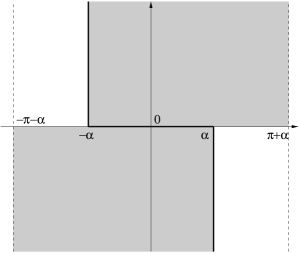
Figure 10: The regularity domain of $\Phi_{1}(\omega)$.

A.3 The domain of regularity and location of singularities of $\Phi_{1}(\omega)$

Let us return to (94). Its left-hand side is regular in the region $\{\mathop{\rm Im\leavevmode\nobreak\ }\nolimits\omega>0,\ 0<\mathop{\rm Re\leavevmode\nobreak\ }\nolimits\omega<\pi\};|\theta|\leq\alpha\}$. Therefore, the function $\Phi_{1}(\omega)$ has no singularities in the half-strip $\{-\alpha<\mathop{\rm Re\leavevmode\nobreak\ }\nolimits\omega<\pi+\alpha,\ \mathop{\rm Im\leavevmode\nobreak\ }\nolimits\omega>0\}$. It can be similarly argued that the half-strip $\{-\pi-\alpha<\mathop{\rm Re\leavevmode\nobreak\ }\nolimits\omega<\alpha,\ \mathop{\rm Im\leavevmode\nobreak\ }\nolimits\omega<0\}$ contains no singularities either (see Fig.  10, where the dashed and solid lines are the boundaries of the two half-strips in which the function $\Phi_{1}(\omega)$ is holomorphic.) However, there might be singularities on the boundaries of these half-strips.

Let us consider the solid lines

$$\{\mathop{\rm Re\leavevmode\nobreak\ }\nolimits\omega=-\alpha,\ \mathop{\rm Im\leavevmode\nobreak\ }\nolimits\omega\geq 0\}\cup\{\mathop{\rm Im\leavevmode\nobreak\ }\nolimits\omega=0,\ -\alpha\leq\omega\leq+\alpha,\}\ \cup\{\mathop{\rm Re\leavevmode\nobreak\ }\nolimits\omega=\alpha,\ \mathop{\rm Im\leavevmode\nobreak\ }\nolimits\omega\leq 0\}.$$ (102)

The singularities which lie on these lines give rise to incoming surface waves. Let us discuss this point in more detail. Let us consider the Sommerfeld integral

$${\int\limits}_{C\cup\tilde{C}}\Phi_{1}(\omega+\theta){\rm e}^{{\rm i}kr{\rm cos\leavevmode\nobreak\ }\omega}{\rm d}\omega.$$ (103)

When evaluating (5), any pole $\omega_{0}$ of $\Phi_{1}(\omega)$, such that $-\alpha<\omega_{0}<\alpha,$ gives rise to a plane wave with the phase factor ${\exp}\leavevmode\nobreak\ [{\rm i}kr{\rm cos\leavevmode\nobreak\ }(\omega_{0}-\theta)]$ (see (104)), that is a plane body wave propagating along the ray $\theta=\omega_{0}$ which lies inside the wedge. By the same token, any pole $\omega_{1}=-\alpha+{\rm i}\beta_{R}$ of $\Phi_{1}(\omega)$, with $\beta_{R}>0$ gives rise to a plane wave with the phase factor

$${\rm e}^{{\rm i}kr{\rm cos\leavevmode\nobreak\ }(\omega_{1}-\theta)}={\rm e}^{{\rm i}kr{\rm cos\leavevmode\nobreak\ }(\alpha+\theta)\cosh\beta_{R}}{\rm e}^{-kr{{\rm sin\leavevmode\nobreak\ }(\alpha+\theta)\sinh\beta_{R}}},$$ (104)

so that its amplitude is exponentially small everywhere except for a small neighbourhood of the wedge face $\theta=-\alpha$. Thus, the pole $\omega_{1}=-\alpha+{\rm i}\beta_{R},\ \beta_{R}>0$ gives rise to the surface (known as Rayleigh) wave which propagates from infinity to the wedge tip along the wedge face $\theta=-\alpha$. Similarly, any pole $\omega_{2}=\alpha-{\rm i}\beta_{R}$ corresponds to the Rayleigh surface wave which propagates from infinity to the wedge tip along the wedge face $\theta=\alpha$.

A.4 The asymptotics of $\Phi_{i}$ at infinity

Let us finish this Appendix by discussing the behaviour of $\Phi_{i}(\omega)$ at infinity. Again we carry out the argument for $\Phi_{1}=\Phi_{1}$ only. The Laplace transform $\overline{\Phi}_{1}(s,\theta)$ has an asymptotic expansion similar to (107), with the expansion coefficients that are functions of $\theta$ (Fedoryuk 1977 and and Osipov and Norris 1999, Theorem 2). Significantly, the $p=0$ terms are either absent or involve constant coefficients (Kozlov et al. 2001). Therefore, the function

$$\Phi_{1}^{\prime}(\omega)=\frac{1}{2}[\partial_{\omega}\Phi_{1}(\omega+\theta)+\partial_{\theta}\Phi_{1}(\omega+\theta)]\Big{|}_{\theta=0}$$ (105)

has the expansion of the type (107) without a constant term. Using (85) this implies that as $\mathop{\rm Im\leavevmode\nobreak\ }\nolimits\omega\rightarrow\infty$, $\Phi_{1}^{\prime}(\omega)\rightarrow 0$ and therefore, $\Phi_{1}(\omega)\rightarrow$ const. When the constant is chosen to be zero (or another specified value) we call the corresponding function $\Phi_{1}(\omega)$ the Sommerfeld amplitude.

Appendix B The tip asymptotics of the elastic potentials and asymptotics of the Sommerfeld amplitudes at infinity

The behavior of solutions of the elliptic problems in regions with piecewise smooth boundaries has been studied by many authors (see Nazarov and Plamenevskij 1994 and references therein). A rigorous theory has been developed after a breakthrough by Kondrat’ev (1963) who constructed and justified the field asymptotics in the vicinity of conical and edge points. The theory implies that the solution of the underlying Lamé problem must have the asymptotic expansion

$${\bf u}(kr,\theta)\sim\sum_{\ell,m=0}^{\infty}(kr)^{q_{m}+2\ell}\sum_{n=0}^{N_{m}-1}{\bf u}_{\ell,m,n}(\theta)\,(\ln kr)^{n},\ \ \ kr\rightarrow 0,$$ (106)

where for one $m$, $q_{m}=0$ and $N_{m}=1$ (otherwise, the tip conditions are violated); and for any other $m$, $\mathop{\rm Re\leavevmode\nobreak\ }\nolimits q_{m}>0$ and $q_{m}$ is a root of a transcendental equation, with a natural number $N_{m}$ being its multiplicity.

The asymptotic expansions (106) can be differentiated and substituted into the boundary conditions. Therefore, using (4) similar expansions may be written for the elastodynamic potentials $\phi^{\pm}_{i}(kr,\theta)$ as

$$\phi^{\pm}_{i}(kr,\theta)\sim\sum\limits_{\ell,m=0}^{\infty}(kr)^{p^{\pm}_{m}+2\ell}\sum\limits_{n=0}^{N_{m}^{\pm}-1}\phi^{\pm}_{i,\ell,m,n}(\theta)(\ln kr)^{n},\,\,\,kr\rightarrow 0.$$ (107)

Let us arrange the sets of exponents $\{p^{+}_{m},\ m=0,1,...$} and $\{p^{-}_{m},\ m=0,1,...\}$, each in order of the increasing real part. Following Kozlov et al. (2001), these sets may be described as follows: Each contains $1$, while any other element is a root of the transcendental equation

$$(p^{\pm}+1)\leavevmode\nobreak\ {\rm sin\leavevmode\nobreak\ }2\alpha\pm{\rm sin\leavevmode\nobreak\ }2\alpha(p^{\pm}+1)=0$$ (108)

and satisfies condition

$$\mathop{\rm Re\leavevmode\nobreak\ }\nolimits p^{\pm}>-1$$ (109)

(otherwise, the tip conditions are violated). Note that if in (106), a $q_{m}\neq 0$, then in (107) the corresponding $p^{+}_{m}$ or $p^{-}_{m}$ equals $q_{m}-1$, but applying the nabla operator to the term with $q_{m}=0$ and $\ell=0$ always gives us zero—because the corresponding $N_{m}=1$. Thus, for $q_{m}=0$, only the next, $r^{2}$, term in (106) gives rise to a nonzero term in (107). The corresponding $p^{\pm}_{m}=1$. Note that while for any wedge angle there exists an $m$, such that $p^{-}_{m}=0$ is a solution of (108), in our range of wedge angles $2\alpha\in(0,\pi)$, all $p^{+}_{m}$ differ from zero. The full set of solutions of the transcendental equations (108) is described in Kozlov et al. (2001). The main facts can be summarized in plots representing roots of the transcendental equations as functions of the wedge angle $2\alpha$ (see e.g. Ting, 1984). The analysis of these plots shows that in our range of wedge angles, the tip conditions are assured for those non-negative exponents with the minimal real part that are either $1$ or else are solutions of the corresponding transcendental equations, with the real part less or equal than $1$. In other words, all leading exponents in (106), that is, the exponents with the minimal real part lie in the strip

$$0\leq{\rm Re}\leavevmode\nobreak\ p^{\pm}_{0}\leq 1.$$ (110)

The root loci in Ting (1984) also show that at one wedge angle, $2\alpha_{*}\approx 0.8\pi$, we have a degeneracy: In the corresponding symmetric problem, the exponent with the minimal real part, $p^{+}_{*}\approx 0.76$ is a multiple root of the corresponding transcendental equation (108). The corresponding multiplicity $N_{*}^{+}=2.$ There are no multiple roots $p^{-}_{0}$ which have the minimal real part and simultaneously satisfy (110). It follows that for $\alpha_{*}$, the leading terms in (106) are

$$\phi^{+}_{i,0,1,1}(kr)^{p^{+}_{*}}{\rm ln}\leavevmode\nobreak\ kr=O\bigl{(}(kr)^{p}\bigr{)},\,\,\,0<p<p^{+}_{*}.$$ (111)

The behavior of potentials $\phi^{\pm}_{i}(kr,\theta)$ in the vicinity of the wedge tip dictates the asymptotic behavior of the Sommerfeld amplitudes $\Phi^{\pm}_{i}(\omega)$ at infinity: For example, it is easy to check that for any small ${\varepsilon}>0$, as $\mathop{\rm Im\leavevmode\nobreak\ }\nolimits\omega\rightarrow\infty,$ $\Phi^{\pm}_{i}(\omega)$ have expansions

$$\Phi^{\pm}_{i}(\omega)\sim\sum_{0\leq\mathop{\rm Re\leavevmode\nobreak\ }\nolimits p^{\pm}_{m}\leq 1}{\Phi}^{\pm}_{im}{\rm e}^{{\rm i}p^{\pm}_{m}\omega}+O({\rm e}^{{\rm i}(1+{\varepsilon})\omega}),\,\,\,\,\alpha\neq\alpha_{*},\ 0<\alpha<\frac{\pi}{2},$$

$$\Phi^{+}_{i}(\omega)\sim{\overline{\Phi}}_{i*}\omega{\rm e}^{{\rm i}p^{+}_{*}\omega}+{\Phi}_{i*}{\rm e}^{{\rm i}p^{+}_{*}\omega}+{\Phi}_{i1}{\rm e}^{{\rm i}\omega}+O({\rm e}^{{\rm i}(2+{\varepsilon})\omega}),\,\,\,\alpha=\alpha_{*}.$$ (112)

Note that in the symmetric case, the expansions contain no constant terms (so that the leading exponents are $1$ and possibly a solution of (108), with the real part in $(0,1)$), but these may be present in the antisymmetric case (so that the leading exponents there are $0$ and $1$).

Appendix C Radiation conditions at infinity

In wedge problems, the radiation conditions at infinity are readily expressed in the form of the limiting absorbtion principle: As $kr\rightarrow\infty$, the diffracted waves ${\bf u}^{\text{diff}}$ with $\mathop{\rm Im\leavevmode\nobreak\ }\nolimits k<0$ should decay exponentially. The solution of the original problem is obtained by taking the limit as $\mathop{\rm Im\leavevmode\nobreak\ }\nolimits k\rightarrow 0$.

Recently a version of the limiting absorbtion principle for the elastic wedge has been justified in Kamotski and Lebeau (2006). As a result, the new radiation conditions have been introduced which are consistent with the physics of the dynamic problem under consideration. The new radiation conditions have allowed the authors to prove that the elastic wedge problem stated in terms of displacements has a unique solution. Reverting to the language of potentials the Kamotski and Lebeau conditions may be re-written as

the inner radiation conditions

$${\int\limits}_{|\theta|<\alpha-(kr)^{-1+\varepsilon}}\left|{\rm i}\gamma k\phi_{0}^{\text{diff}}+\partial_{r}\phi_{0}^{\text{diff}}\right|^{2}\,r{\rm d}\theta\rightarrow 0,$$ (113)

$${\int\limits}_{|\theta|<\alpha-(kr)^{-1+\varepsilon}}\left|{\rm i}k\phi_{1}^{\text{diff}}+\partial_{r}\phi_{1}^{\text{diff}}\right|^{2}\,r{\rm d}\theta\rightarrow 0,\ kr\rightarrow\infty$$ (114)

surface radiation conditions

$$\int\limits_{\alpha-(kr)^{-1+\varepsilon}\leq|\theta|\leq\alpha}\left|{\rm i}k_{R}\phi_{i}^{\text{diff}}+\partial_{r}\phi_{i}^{\text{diff}}\right|^{2}\,r{\rm d}\theta\rightarrow 0, r\rightarrow\infty,$$ (115)

where $k_{R}=\Omega/c_{R}$ plus the requirement that as $kr\rightarrow\infty$ the diffracted field satisfies the boundedness condition. Following the methods of Kamotski and Lebeau (2006) it must be possible to show that the same conditions are sufficient for proving uniqueness of the elastic wedge diffraction problem stated in terms of elastodynamic potentials.

Appendix D Geometrico-elastodynamic poles of $\Phi_{i}$

In this Appendix we present recursive formulae for evaluating the geometrico-elastodynamic poles of $\Phi_{i}(\omega)$ with the corresponding residues.

D.1 The symmetric problem

Given an incident P (compressional) wave

$$\phi_{0}^{\text{inc}}(kr,\theta)={\rm e}^{{\rm i}[\gamma kr{\rm cos\leavevmode\nobreak\ }(\theta-\theta_{0}^{\text{inc}})]},$$ (116)

the symmetric function $\Phi_{0}^{+}(\omega)$ has two poles at the angles of incidence $\theta_{01}$ and $\theta_{02}$, with the corresponding residues $\mathop{\rm Res\leavevmode\nobreak\ }\nolimits\Phi_{0}^{+}(\theta_{0\ell}),\,\ell=1,2$. These are

$$\theta_{01}=-\theta_{0}^{\text{inc}},\leavevmode\nobreak\ \leavevmode\nobreak\ \theta_{02}=\theta_{0}^{\text{inc}},$$

$$\mathop{\rm Res\leavevmode\nobreak\ }\nolimits\Phi_{0}^{+}(\theta_{0\ell})=-\frac{1}{4\pi{\rm i}}.$$ (117)

The poles lie in the strip $|\mathop{\rm Re\leavevmode\nobreak\ }\nolimits\omega|\leq\alpha$. It follows from the first equation in (31) that $\Phi_{0}^{+}(\omega)$ also has P-P poles $\theta_{0\ell},\,\ell=3,4$, with the respective residues $\mathop{\rm Res\leavevmode\nobreak\ }\nolimits\Phi_{0}^{+}(\theta_{0\ell})$. These describe the once reflected compressional wave and are given by

$$\theta_{0\ell}=\theta_{0,\ell-2}+2\alpha,$$

$$\mathop{\rm Res\leavevmode\nobreak\ }\nolimits\Phi_{0}^{+}(\theta_{0\ell})={\rm r}_{11}(g^{-1}(\theta_{0,\ell-2}+\alpha))\mathop{\rm Res\leavevmode\nobreak\ }\nolimits\Phi_{0}^{+}(\theta_{0,\ell-2}).$$ (118)

The S (shear) waves generated on the first reflection are associated with the P-S poles $\omega=\theta_{1\ell},\,\ell=3,4$, with the corresponding residues $\mathop{\rm Res\leavevmode\nobreak\ }\nolimits\Phi_{1}^{+}(\theta_{1\ell}).$ These are given by

$$\theta_{1\ell}=g^{-1}(\theta_{0,\ell-2}+\alpha)+\alpha$$

$$\mathop{\rm Res\leavevmode\nobreak\ }\nolimits\Phi_{1}^{+}(\theta_{1\ell})=\frac{{\rm r}_{21}(g^{-1}(\theta_{0,\ell-2}+\alpha))}{g^{\prime}(\theta_{1\ell}-\alpha)}\mathop{\rm Res\leavevmode\nobreak\ }\nolimits\Phi_{0}^{+}(\theta_{0,\ell-2}).$$ (119)

Similarly, the poles $\theta_{0\ell}$ and $\theta_{1\ell},\,\ell=5,6$ of the type P-P-P and P-P-S are described by formulae (118) and (119) respectively. The P-S-P poles $\theta_{0\ell},\,\ell=7,8$ are given by

$$\theta_{0\ell}=g(\theta_{1,\ell-4}+\alpha)+\alpha$$

$$\mathop{\rm Res\leavevmode\nobreak\ }\nolimits\Phi_{0}^{+}(\theta_{0\ell})={\rm r}_{12}(\theta_{1,\ell-4}+\alpha)g^{\prime}(\theta_{1,\ell-4}+\alpha)\mathop{\rm Res\leavevmode\nobreak\ }\nolimits\Phi_{1}(\theta_{1,\ell-4}),$$ (120)

and P-S-S poles $\theta_{1\ell},\,\ell=7,8$ by

$$\theta_{1\ell}=\theta_{1,\ell-4}+2\alpha,$$

$$\mathop{\rm Res\leavevmode\nobreak\ }\nolimits\Phi_{1}^{+}(\theta_{1\ell})={\rm r}_{22}(\theta_{1,\ell-4}+\alpha)\mathop{\rm Res\leavevmode\nobreak\ }\nolimits\Phi_{1}^{+}(\theta_{1,\ell-4}).$$ (121)

The above formulae should be applied recursively until one evaluates all poles within (8). Due to the symmetry of $\Phi_{0}^{+}(\omega)$ and $\Phi_{1}^{+}(\omega),$ $-\theta^{ik}$ are their respective poles as well, with the corresponding residues ${\rm Res\leavevmode\nobreak\ }\Phi_{0}^{+}(-\theta_{0\ell})={\rm Res\leavevmode\nobreak\ }\Phi_{0}^{+}(\theta_{0\ell})$ and ${\rm Res\leavevmode\nobreak\ }\Phi_{1}^{+}(-\theta_{1\ell})=-{\rm Res\leavevmode\nobreak\ }\Phi_{1}^{+}(\theta_{1\ell})$. If the recursive procedure is initiated outside the strip $|\mathop{\rm Re\leavevmode\nobreak\ }\nolimits\omega|\leq\alpha$, then, as equations (31) suggest, other pairs of poles appear to be possible. However, direct calculations show that such points give a zero contribution.

D.2 The antisymmetric problem

The antisymmetric problem allows a similar treatment, the analytic continuation should also be performed using Eq. (31) with the “$-$” superscipt.

Appendix E The integral equations for one unknown

Symmetric problem

The two final regularized integral equations to solve are

$$\widetilde{y}^{+}_{i}(\eta)+\widetilde{L}^{+}\widetilde{y}^{+}_{i}(\eta)=\widetilde{q}^{+}_{i}(\eta),\,\,i=0,1,$$ (122)

where $\widetilde{L}^{+}$ is an operator with a smooth kernel

$$(\widetilde{L}^{+}u)(\eta) =-\frac{1}{4\alpha^{2}}{\int\limits_{-\infty}^{\infty}}{l^{+}(\eta,t)\tanh 2t\over\sqrt{d(t)}\sqrt{d(\eta)}\cosh\frac{\displaystyle\pi}{\displaystyle 2\alpha}\eta}u(t)\,dt,$$ (123)

with

$$l^{+}(\eta,t)=\text{V.P.}{\int\limits_{-\infty}^{\infty}}{\cosh\frac{\displaystyle\pi}{\displaystyle 2\alpha}\tau\over\sinh\frac{\displaystyle\pi}{\displaystyle 2\alpha}(\tau-\eta)}\Big{\{}{\tanh 2t\over\chi^{\prime}(t)\sinh\frac{\displaystyle\pi}{\displaystyle 2\alpha}(t-\tau)}-{\tanh 2\tau\over\sinh\frac{\displaystyle\pi}{\displaystyle 2\alpha}[\chi(t)-\chi(\tau)]}\Big{\}}\,d\tau.$$

The respective right hand sides of Eqs. (122) are given by

$$\widetilde{q}^{+}_{i}(\eta)=\frac{1}{\displaystyle 2\alpha{\rm i}\sqrt{d(\eta)}\cosh\frac{\displaystyle\pi}{\displaystyle 2\alpha}\eta}\text{V.P.}\displaystyle{\int\limits_{-\infty}^{\infty}}\frac{\cosh\frac{\displaystyle\pi}{\displaystyle 2\alpha}t}{\sinh\frac{\displaystyle\pi}{\displaystyle 2\alpha}(t-\eta)}q^{+}_{i}(t)\,dt,\,\,$$ (124)

with $q_{i}^{+}(\eta)$ given in Appendix I. On solving (122), $y^{+}(\eta)$ is obtained using

$$y^{+}(\eta)=d^{-1/2}(\eta)[\widetilde{y}^{+}_{0}(\eta)+c^{+}_{1}\widetilde{y}^{+}_{1}(\eta)],$$ (125)

where $c^{+}_{1}=-\lambda^{+}_{0}/\lambda^{+}_{1}$ and we have

$$\lambda^{+}_{i}={\int\limits_{-\infty}^{\infty}}\bigl{[}\widetilde{y}^{+}_{i}(t)d^{-1/2}(t)(B^{+}{\mathbb{I}})(t)-q^{+}_{i}(t)\bigr{]}dt,\,\,\,i=0,1,$$

$$(B^{+}{\mathbb{I}})(t)=\frac{\gamma^{2}\tanh 2t}{2\alpha{\rm i}}{\int\limits_{-\infty}^{\infty}}\frac{\sinh 2(\chi(t)+\tau)}{1+2\gamma^{2}\sinh^{2}(\tau+\chi(t))}\,\cdot\,\frac{d\tau}{\sinh\frac{\displaystyle\pi}{\displaystyle 2\alpha}\tau}.$$

Antisymmetric problem

Analogously to the symmetric case, the two final regularized integral equations to solve are

$$\widetilde{x}_{i}^{-}(\eta)+\widetilde{L}^{-}\widetilde{x}_{i}^{-}(\eta)=\widetilde{q}_{i}^{-}(\eta),\,\,i=0,1,$$ (126)

where the integral operator is

$$(\widetilde{L}^{-}u)(\eta) =-\frac{1}{4\alpha^{2}}{\int\limits_{-\infty}^{\infty}}{l^{-}(\eta,t)\tanh 2t\over\sqrt{d(t)}\sqrt{d(\eta)}\cosh\frac{\displaystyle\pi}{\displaystyle 2\alpha}\chi(\eta)}u(t)\,dt,$$ (127)

with

$$\ \ \ l^{-}(\eta,t)=-\text{V.P.}{\int\limits_{-\infty}^{\infty}}{\cosh\frac{\displaystyle\pi}{\displaystyle 2\alpha}\tau\over\sinh\frac{\displaystyle\pi}{\displaystyle 2\alpha}[\chi(\eta)-\tau]}\Big{\{}{\tanh 2t\over\sinh\frac{\displaystyle\pi}{\displaystyle 2\alpha}(\chi(t)-\tau)}+\frac{\tanh 2\chi^{-1}(\tau)({{\chi^{-1}}})^{\prime}(\tau)}{\sinh\frac{\displaystyle\pi}{\displaystyle 2\alpha}[\chi^{-1}(\tau)-t]}\Big{\}}\,d\tau.$$

The respective right hand sides of Eqs. (126) are given by

$$\widetilde{q}_{i}^{-}(\eta)=\frac{1}{2\displaystyle\alpha{\rm i}\sqrt{d(\eta)}\cosh\frac{\displaystyle\pi}{\displaystyle 2\alpha}\chi(\eta)}\text{V.P.}\displaystyle{\int\limits_{-\infty}^{\infty}}\frac{\cosh\frac{\displaystyle\pi}{\displaystyle 2\alpha}t}{\sinh\frac{\displaystyle\pi}{\displaystyle 2\alpha}[t-\chi(\eta)]}q_{i}^{-}(\chi^{-1}(t))\,dt,\,\,$$ (128)

with $q_{i}^{-}(\eta)$ given in Appendix I. As above, $x^{-}$ is obtained on solving (126) using

$$x^{-}(\eta)=d^{-1/2}(\eta)[\widetilde{x}_{0}^{-}(\eta)+c_{1}^{-}\widetilde{x}_{1}^{-}(\eta)],$$ (129)

where $c_{1}^{-}=-\lambda_{0}^{-}/\lambda_{1}^{-}$ and we have

$$\lambda_{i}^{-}={\int\limits_{-\infty}^{\infty}}\bigl{[}\widetilde{x}_{i}^{-}(t)d^{-1/2}(t)(B^{-}\chi^{\prime})(t)-q_{i}^{-}(t)\chi^{\prime}(t)\bigr{]}dt,\,\,i=0,1,$$

$$(B^{-}\chi^{\prime})(t)=\frac{\tanh 2t}{2\alpha{\rm i}}\int_{-\infty}^{\infty}\frac{\tanh 2(t+\tau)\,d\tau}{\sinh\frac{\displaystyle\pi}{\displaystyle 2\alpha}\tau}.$$

Appendix F The branch points of $\Phi_{i}(\omega)$

Let us show that the Sommerfeld amplitudes $\Phi^{+}_{i}(\omega)$ that satisfy the functional equations (13) and conditions(9) can have only physically meaningful branch points. For simplicity of presentation, let us assume that $\theta_{h}<2\alpha$ (in the opposite case, a slightly more involved argument still goes through.) Using the branch points of $g(\omega)$, the only branch points that $\Phi_{1}^{+}(\omega)$ can have inside (8) are $\pm(\pi+\alpha-\theta_{h})$. The corresponding branch cuts run along the segments $[-\pi-\alpha-\theta_{h},\leavevmode\nobreak\ -\pi-\alpha+\theta_{h}]$ and $[\pi+\alpha-\theta_{h},\leavevmode\nobreak\ \pi+\alpha+\theta_{h}]$. Note that the branch points $\pm(\pi+\alpha+\theta_{h})$ lie outside the physical region (8). The analogous branch points of $\Phi_{0}^{+}(\omega)$ can be only $\pm(\pi+\alpha\pm{\rm i}{\cosh^{-1}}(1/\theta_{h}))$, with the cuts along the segments $[-\pi-\alpha+{\rm i}{\cosh^{-1}\leavevmode\nobreak\ }(1/\theta_{h}),\leavevmode\nobreak\ -\pi-\alpha-{\rm i}{\cosh^{-1}\leavevmode\nobreak\ }(1/\theta_{h})]$ and $[\pi+\alpha+{\rm i}{\cosh^{-1}\leavevmode\nobreak\ }(1/\theta_{h}),\leavevmode\nobreak\ \pi+\alpha-{\rm i}{\cosh^{-1}\leavevmode\nobreak\ }(1/\theta_{h})]$.

Indeed, all possible branch points of $g(\omega)$ are $\pi n\pm\theta_{h}$ (see (15)). In principle, applying (13), they could generate many branch points in $\Phi_{1}^{+}(\omega)$ which have no physical interpretation. Let us start by showing that $-\alpha+\theta_{h}$ is not a branch point: Let us use the fact that $\Phi_{0}^{+}(\omega)$ is odd to rewrite the functional equation (13) as

$$t_{11}(\omega+\alpha)\{\Phi_{0}^{+}[\alpha+g(\omega+\alpha)]-\Phi_{0}^{+}[\alpha-g(\omega+\alpha)]\}+t_{12}(\omega+\alpha)[\Phi_{1}^{+}(\omega+2\alpha)+\Phi_{1}^{+}(\omega)]=Q_{1}^{+},$$ (130)

$$t_{21}(\omega+\alpha)\{\Phi_{0}^{+}[\alpha+g(\omega+\alpha)]+\Phi_{1}^{+}[\alpha-g(\omega+\alpha)]\}+t_{22}(\omega+\alpha)[\Phi_{1}^{+}(\omega+2\alpha)-\Phi_{1}^{+}(\omega)]=Q_{1}^{+}.$$ (131)

In the vicinity of $\theta_{h}$, there exist the constants $a_{n}$ such that we have

$$g(\omega+\alpha)=\sum_{n=0}^{\infty}a_{n}(\omega+\alpha-\theta_{h})^{n+1/2}.$$ (132)

Since $\Phi_{0}^{+}[\alpha+g(\omega+\alpha)]-\Phi_{0}^{+}[\alpha-g(\omega+\alpha)]$ is odd in $g$, there also exist constants $A_{n}$ such that that this function has the expansion

$$\Phi_{0}^{+}[\alpha+g(\omega+\alpha)]-\Phi_{0}^{+}[\alpha-g(\omega+\alpha)]=\sum_{n=0}^{\infty}A_{n}(\omega+\alpha-\theta_{h})^{n+1/2}.$$ (133)

On the other hand, there exist constants $b_{n}$ such that we can write

$$t_{11}(\omega+\alpha)=\sum_{n=0}^{\infty}b_{n}(\omega+\alpha-\theta_{h})^{n-1/2}.$$ (134)

Thus, the first term in the left hand side of (130) contains no branch points. The coefficient $t_{12}$ has no branch points either. It follows that there are no branch points in Eq. (130) at all.

Let us move on to Eq. (131). The function $\Phi_{0}^{+}[\alpha+g(\omega+\alpha)]+\Phi_{0}^{+}[\alpha-g(\omega+\alpha)]$ is an even function of $g$, and therefore, there exist constants $B_{n}$ such that we can write

$$\Phi_{0}^{+}[\alpha+g(\omega+\alpha)]+\Phi_{0}^{+}[\alpha-g(\omega+\alpha)]=\sum_{n=0}^{\infty}B_{n}(\omega+\alpha-\theta_{h})^{n}.$$ (135)

Since the coefficients $t_{21}(\omega)$ and $t_{22}(\omega)$ have no branch points, there are no branch points in Eq. (131). It follows that the point $-\alpha+\theta_{h}$ which does not have any physical interpretation is not a branch point of the function $\Phi_{1}^{+}(\omega)$. Similarly, it can be shown that the points $-\alpha-\theta_{h}$ and $\alpha\pm\theta_{h}$ are not branch points of $\Phi_{1}^{+}(\omega)$. Analogous considerations apply in the antisymmetric case.

We conclude that the branch points of the Sommerfeld amplitudes of the solution of the original problem that lie in the physical region (8) and therefore give rise to physical waves, lie outside the strip $\mathop{\rm Re\leavevmode\nobreak\ }\nolimits\omega\,\epsilon\,I$. This means that they do not have to be taken into account in the functional equations for ${\widetilde{\Phi}}^{\pm}_{i}(\omega)$ or by the same token, in the resulting singular integral problem. On the other hand, we have no theoretical proof that $\Phi^{\pm}_{i}(\omega)$ that we eventually compute have only physical branch points in the physical region(8). We can confirm this fact only by carrying out numerical tests.

Appendix G The Rayleigh reflection and transmission coefficients

When evaluating (5), a pole $\theta^{{\rm inc}}_{1{\rm R}}=\alpha-{\rm i}\beta_{\rm R}$ of $\Phi_{1}(\omega)$, with $\beta_{\rm R}>0$ corresponds to a plane wave with the phase factor

$${\rm e}^{{\rm i}kr{\rm cos\leavevmode\nobreak\ }(\theta-\theta^{{\rm inc}}_{1{\rm R}})}={\rm e}^{{\rm i}kr{\rm cos\leavevmode\nobreak\ }(\theta-\alpha)\cosh\beta_{\rm R}}{\rm e}^{-kr{{\rm sin\leavevmode\nobreak\ }(\alpha-\theta)\sinh\beta_{\rm R}}},$$ (136)

so that its amplitude is exponentially small everywhere except for a small neighborhood of the wedge face $\theta=\alpha$. Thus, we describe a Rayleigh wave incident from infinity along the upper face $\theta=\alpha$ by two potentials

$$\phi^{\text{inc}}_{i}(kr,\theta)=4\pi{\rm i}\phi_{i0}{\rm e}^{{\rm i}\gamma kr{\rm cos}(\theta-\theta^{{\rm inc}}_{i{\rm R}})},$$ (137)

where $\phi_{00}=1$ and $\phi_{10}={\displaystyle-2{\rm i}\gamma_{\rm R}\sqrt{\gamma_{\rm R}^{2}-\gamma^{2}}}/({\displaystyle 2\gamma_{\rm R}^{2}-1})$; $\gamma_{\rm R}=c_{\rm S}/c_{\rm R}$ with $c_{\rm S}$ being the Rayleigh wave speed and $\theta^{{\rm inc}}_{0{\rm R}}=\alpha-g({\rm i}\beta_{\rm R})$. The reflected wave propagates along the same wedge face as the incident but from the tip to infinity and transmitted—along the other face, again away from the tip. They are described respectively by

$$\phi^{\rm ref}_{i}(kr,\theta)=4\pi{\rm i}R^{\rm ref}\phi_{i0}{\rm e}^{-{\rm i}\gamma kr{\rm cos}(\theta-\theta^{{\rm sc}}_{i{\rm R}})},$$

$$\phi^{\rm tran}_{i}(kr,\theta)=4\pi{\rm i}R^{\rm tran}\phi_{i0}{\rm e}^{-{\rm i}\gamma kr{\rm cos}(\theta+\theta^{{\rm sc}}_{i{\rm R}})},$$ (138)

with “scattering angles” $\theta^{{\rm sc}}_{i{\rm R}}$ being the complex conjugate of $\theta^{{\rm inc}}_{i{\rm R}}$, so that $\theta^{{\rm sc}}_{0{\rm R}}=\alpha+g({\rm i}\beta_{\rm R})$ and $\theta^{{\rm sc}}_{1{\rm R}}=\alpha+{\rm i}\beta_{\rm R}$. Above, $R^{\rm ref}$ and $R^{\rm tran}$ are the Rayleigh reflection and transmission coefficients

$$R^{\text{\rm ref}}=\frac{1}{2}[R^{\text{+ref}}+R^{-\text{ref}}],\,\,\,R^{\text{\rm tran}}=\frac{1}{2}[R^{\text{+ref}}-R^{-\text{ref}}],$$ (139)

with the symmetric and antisymmetric parts given respectively by

$$R^{\pm\text{\rm ref}}=\text{Res}[\Phi_{0}^{\pm};\,g(\omega_{\rm R})+\alpha],\,\,\,{\rm with\leavevmode\nobreak\ }\omega_{\rm R}=\pi+{\rm i}\beta_{\rm R},$$ (140)

so that using the additional angles $\theta_{0,{\rm R}}=-\alpha+g(\omega_{\rm R})$ and $\theta_{1,{\rm R}}=-\alpha+\omega_{\rm R}$, we have

$$R^{\pm\text{ref}}=\pm\sum_{k=1}^{2}{\rm r}_{1k}(\omega_{\rm R})\Phi^{\pm}_{k-1}(\theta_{k-1,{\rm R}})+c_{1}^{\pm}e^{\pm}_{1}(\omega_{\rm R})\frac{g^{\prime}(\omega_{\rm R})\Delta(\omega_{\rm R})}{\Delta^{\prime}(\omega_{\rm R})}\sqrt{\gamma^{2}-{\rm cos}^{2}\omega_{\rm R}}.$$

As before, the dash denotes the derivative with respect to the argument.

Appendix H Adjustable functions and parameters in singular terms

As any other numerical code ours relies on a choice of certain options which effect a tradeoff between numerical accuracy and either running time or else numerical stability. Apart from the relevant grids, these options are

1. The adjustable function $\sigma(\omega)$ in (32) In most cases, $\sigma(\omega)$ is chosen to be

   $$\sigma(\omega)=\frac{\frac{\displaystyle\pi}{\displaystyle 2\alpha}}{{\rm sin\leavevmode\nobreak\ }\frac{\displaystyle\pi}{\displaystyle 2\alpha}\omega}$$ (141)

   (cf. Budaev and Bogy 1995, Eq. (15)). The choice is convenient, because it simplifies the right hand sides of our functional and therefore, integral equations. Also, $\sigma(\omega)$ in (141) decays at infinity reasonably fast. However, for any wedge angle $2\alpha$, there exists a critical incident angle $\theta^{\text{inc}}_{0}$, such that one of the poles of $\Phi^{\pm}_{i}(\omega)$ lies on the boundary of the strip $\mathop{\rm Re\leavevmode\nobreak\ }\nolimits\omega\,\epsilon\,I$. For illustration purposes, let it be $\widehat{\Phi}^{\pm}_{1}(\omega)$ and let the pole be $\theta_{0}=\pi/2-\alpha$. Then the corresponding term ${\rm Res\leavevmode\nobreak\ }(\Phi^{\pm}_{1};\theta_{0})\sigma(\omega-\theta_{0})$ has one more nonphysical pole, $\theta_{0}+2\alpha$. In situations like these, another choice of $\sigma(\omega)$ is called for, with poles further apart. We have tested

   $$\sigma(\omega)=\frac{\beta}{{\rm sin\leavevmode\nobreak\ }\beta\omega}.$$ (142)

   with various values $\beta<\pi/(2\alpha)$. However, any $\sigma(\omega)$ different from (141) leads to more cumbersome right hand sides of the integral equations and exhibits a slower decay. As a result, the function (142) while increasing the stability of the solution, increases the code run time roughly tenfold. For this reason, we abandon (141) only when $\theta^{\text{inc}}$ is near critical angle. In this region we use (142), with $\beta=\pi/(6\alpha)$.

2. Number of poles. When evaluating the poles of the Sommerfeld amplitudes we do not have to restrict ourselves to the strip $\mathop{\rm Re\leavevmode\nobreak\ }\nolimits\omega\,\epsilon\,I$. The more poles that are utilized in evaluation, the wider the domain of analyticity of the corresponding unknowns ${\widetilde{\Phi}}_{i}(\omega)$ and therefore, the higher the accuracy. On the other hand, some nonphysical poles possess residues with large amplitudes and cause numerical instability. In the present version of the code, when $\theta$ is away from critical we take into account all poles in the strip $\mathop{\rm Re\leavevmode\nobreak\ }\nolimits\omega\,\epsilon\,I$, and when $\theta$ is near critical we take into account all poles in the wider strip $\mathop{\rm Re\leavevmode\nobreak\ }\nolimits\omega\,\epsilon\,[\pi/2-2\alpha,\,\pi/2+2\alpha]$.

Appendix I Nomenclature

$$a(\eta)=-{\rm i}\tanh 2\eta,$$

$$b(\eta)=\frac{2{\rm i}\sinh\eta\sqrt{\gamma^{2}+\sinh^{2}\eta}}{\cosh 2\eta},$$

$$d(\eta)=1-\frac{\tanh^{2}2\eta}{\chi^{\prime}(\eta)},$$

$$e^{+}_{1}(\omega)=-\tan\alpha\,{\rm sin\leavevmode\nobreak\ }2\omega+{\rm cos\leavevmode\nobreak\ }2\omega,$$

$$e^{-}_{1}(\omega)=\tan\alpha\,{\rm cos\leavevmode\nobreak\ }2\omega+{\rm sin\leavevmode\nobreak\ }2\omega,$$

$$e^{+}_{2}(\omega)=\tan\alpha\,{\rm cos\leavevmode\nobreak\ }2\omega\frac{{\rm sin\leavevmode\nobreak\ }\omega}{\sqrt{\gamma^{2}-{\rm cos}^{2}\,\omega}}+{\rm sin\leavevmode\nobreak\ }2\omega,$$

$$e^{-}_{2}(\omega)=\tan\alpha\,{\rm sin\leavevmode\nobreak\ }2\omega-{\rm cos\leavevmode\nobreak\ }2\omega\frac{{\rm sin\leavevmode\nobreak\ }\omega}{\sqrt{\gamma^{2}-{\rm cos}^{2}\,\omega}},$$

$$g(\omega)={\rm cos}^{-1}(\gamma^{-1}{\rm cos\leavevmode\nobreak\ }\omega),$$

$${\mathcal{H}}f(\eta)=\frac{1}{2\alpha{\rm i}}\text{V.P.}{\int\limits_{-\infty}^{\infty}}\frac{f(t){\rm d}t}{\sinh[\frac{\pi}{2\alpha}(t-\eta)]},$$

$$({\mathcal{H}}^{-1}f)(\eta)=\frac{1}{2\alpha{\rm i}}\text{V.P.}{\int\limits_{-\infty}^{\infty}}\coth\frac{\displaystyle\pi}{\displaystyle 2\alpha}(t-\eta)f(t)\,dt,$$

$${\overline{\mathcal{H}}}f(\eta)=\frac{1}{2\alpha{\rm i}}\text{V.P.}{\int\limits_{-\infty}^{\infty}}\frac{f(t)\chi^{\prime}(t){\rm d}t}{\sinh\frac{\displaystyle\pi}{\displaystyle 2\alpha}[\chi(t)-\chi(\eta)]},$$

$$Kf(\eta)=\frac{1}{2\alpha{\rm i}}{\int\limits_{-\infty}^{\infty}}\left\{\frac{\tanh^{2}2t}{\chi^{\prime}(t)\sinh\frac{\displaystyle\pi}{\displaystyle 2\alpha}(t-\eta)}-\frac{\tanh 2t\tanh 2\eta}{\sinh\frac{\displaystyle\pi}{\displaystyle 2\alpha}[\chi(t)-\chi(\eta)]}\right\}f(t)\,dt,$$

$$q_{0}^{+}(\eta)=r_{2}^{+}(\eta)-a(\eta){\overline{\mathcal{H}}}r_{1}^{+}(\eta),$$

$$q_{1}^{+}(\eta)=-\tan\alpha\frac{\cosh\eta}{\cosh 2\eta}-\frac{\tanh 2\eta}{2\alpha}\text{V.P.}{\int\limits_{-\infty}^{\infty}}\frac{\gamma\cosh\tau d\tau}{(1+2\gamma^{2}\sinh^{2}\tau)\sinh\frac{\displaystyle\pi}{\displaystyle 2\alpha}[\tau-\chi(\eta)]},$$

$$q_{0}^{-}(\eta)=r_{1}^{-}(\eta)-b(\eta){\mathcal{H}}r_{2}^{-}(\eta),$$

$$q_{1}^{-}(\eta)=-\tan\alpha\frac{\cosh\eta}{\chi^{\prime}(\eta)\cosh 2\eta}-\frac{\tanh 2\eta}{2\alpha\chi^{\prime}(\eta)}\text{V.P.}{\int\limits_{-\infty}^{\infty}}\frac{\cosh\tau\,d\tau}{\cosh 2\tau\,\sinh\frac{\displaystyle\pi}{\displaystyle 2\alpha}(\tau-\eta)},$$

$$r_{1}^{\pm}(\eta)=-\Big{[}\widehat{\Phi}_{0}^{+}(g(\frac{\pi}{2}+{\rm i}\eta)+\alpha)\pm\widehat{\Phi}_{0}^{+}(g(\frac{\pi}{2}+{\rm i}\eta)-\alpha)\Big{]}-b(\eta)\Big{[}\widehat{\Phi}_{1}^{+}(\frac{\pi}{2}+\alpha+{\rm i}\eta)\pm\widehat{\Phi}_{1}^{+}(\frac{\pi}{2}-\alpha+{\rm i}\eta)\Big{]},$$

$$r_{2}^{\pm}(\eta)=-a(\eta)\Big{[}\widehat{\Phi}_{0}^{+}(g(\frac{\pi}{2}+{\rm i}\eta)+\alpha)\mp\widehat{\Phi}_{0}^{+}(g(\frac{\pi}{2}+{\rm i}\eta)-\alpha)\Big{]}-\Big{[}\widehat{\Phi}_{1}^{+}(\frac{\pi}{2}+\alpha+{\rm i}\eta)\mp\widehat{\Phi}_{1}^{+}(\frac{\pi}{2}-\alpha+{\rm i}\eta)\Big{]},$$

$${\rm r}_{11}(\omega)=-{\rm r}_{22}(\omega)=\frac{2{\rm sin\leavevmode\nobreak\ }2\omega\leavevmode\nobreak\ {\rm cos\leavevmode\nobreak\ }\omega\sqrt{\gamma^{2}-{\rm cos}^{2}\leavevmode\nobreak\ \omega}-{\rm cos}^{2}\leavevmode\nobreak\ 2\omega}{\Delta(\omega)},$$

$${\rm r}_{12}(\omega)=-\frac{4{\rm cos\leavevmode\nobreak\ }2\omega\leavevmode\nobreak\ {\rm cos\leavevmode\nobreak\ }\omega\sqrt{\gamma^{2}-{\rm cos}^{2}\leavevmode\nobreak\ \omega}}{\Delta(\omega)},\leavevmode\nobreak\ \leavevmode\nobreak\$$

$${\rm r}_{21}(\omega)=-\frac{2{\rm sin\leavevmode\nobreak\ }2\omega\leavevmode\nobreak\ {\rm cos\leavevmode\nobreak\ }2\omega}{\Delta(\omega)},$$

$$\Delta(\omega)={\rm cos}^{2}\leavevmode\nobreak\ 2\omega+2\leavevmode\nobreak\ {\rm sin\leavevmode\nobreak\ }2\omega\leavevmode\nobreak\ {\rm cos\leavevmode\nobreak\ }\omega\sqrt{\gamma^{2}-{\rm cos}^{2}\leavevmode\nobreak\ \omega},$$

$$\chi(\eta)=\sinh^{-1}(\gamma^{-1}\sinh(\eta)),$$

$$\chi^{\prime}(\eta)=\frac{\cosh\eta}{\sqrt{\gamma^{2}+\sinh^{2}\eta}}.$$

Note that the Rayleigh function $\Delta(\omega)$ has the purely imaginary root ${\rm i}\beta_{\rm R}$, with $\beta_{\rm R}>0$.

References

- [1] K. E. Atkinson, The Numerical Solutions of Integral Equations of the Second Kind. Cambridge University Press, Cambridge, 1997.
- [2] B. V. Budaev, Diffraction by Wedges. Longman Scientific and Technical, Harlow, 1995.
- [3] B. V. Budaev and D. B. Bogy, Rayleigh wave scattering by a wedge, Wave Motion, 22 (1995), pp. 239–257.
- [4] Rayleigh wave scattering by a wedge II, Wave Motion, 24 (1996), pp. 307–314.
- [5] Rayleigh wave scattering by two adhering elastic wedges, Proc. Roy. Soc. Lond. A, 454 (1998), pp. 2949–2996.
- [6] Errata to the paper ‘Rayleigh wave scattering by a wedge II’, Wave Motion, 35 (2002), p. 275.
- [7] H. S. Carslaw, Diffraction of waves by a wedge of any angle. Proc. Lond. Math. Soc. S.2, 18 (1920), pp. 291–306.
- [8] J.-P. Croisille and G. Lebeau, Diffraction by an Immersed Elastic Wedge, Lecture notes in mathematics, Vol. 1723, Springer-Verlag, Berlin, 1999.
- [9] A. M. J. Davis, Point-source excitation of the density contrast wedge: Perturbation for nearly equal sound speeds, Q. J. Mech. Appl.Math., 54 (2001), pp. 613-630.
- [10] M. V. Fedoryuk, The saddle-point method, Nauka, Moscow, 1977. In Russian.
- [11] A. F.Filippov, A three-dimensional problem of diffraction of an elastic wave at a sharp edge, PMM - J. Appl. Math. Mech., 23 (1959), pp. 989-996. In Russian.
- [12] P. Frank and R. von Mises, Differentsial’nye i integral’nye uravneniya matematicheskoi fisiki, Vol. II, ONTI, Leningrad, 1937. In Russian.
- [13] M. M Friedman, Diffraction of an elastic plane wave from a semi-infinite rigid screen, Uch. Zap. Leningr. Univ. Ser. Math. Sci., 17 (1949), pp. 72-94. In Russian.
- [14] M. M. Friedman, Diffraction of an elastic plane wave from a semi-infinite traction free screen, Dokl. Acad. Nauk. USSR, 66 (1949), pp. 21-24. In Russian.
- [15] K. Fujii, Rayleigh-wave scattering of various wedge corners: Investigation in the wider range of wedge angles, Bull. Seismol. Soc. Am., 84 (1994), pp. 1916–1924.
- [16] A. K. Gautesen, Scattering of Rayleigh wave by an elastic quarter space, J. Appl. Mech., 52 (1985), pp. 664–668.
- [17] A. K. Gautesen, Scattering of an obliquely incident Rayleigh wave by an elastic quarter space, Wave Motion, 8 (1986), pp. 27-41.
- [18] A. K. Gautesen, Scattering of a Rayleigh wave by an elastic wedge whose angle is greater than 180 degrees, J. Appl. Mech., 68 (2001), pp. 476-479.
- [19] Scattering of a Rayleigh wave by an elastic quarter space—revisited, Wave Motion, 35 (2002), pp. 91–98.
- [20] A. K. Gautesen, Scattering of a Rayleigh wave by an elastic three-quarter space, Wave Motion, 35 (2002), pp. 99–106.
- [21] Scattering of a Rayleigh wave by an elastic wedge whose angle is less then , Wave Motion, 36 (2002), pp. 417–424.
- [22] V. V. Kamotski, On the Incidence of the Plane Wave on an Elastic Wedge at a Critical Angle, Algebra and Analysis, 15 (2003), pp. 145–169. [English transl.: St. Petersburg Math. J., 15, pp. 419–436.]
- [23] V. V. Kamotski and G. Lebeau, Diffraction by an elastic wedge with stress free boundary: Existence and uniqueness, Proc. Roy. Soc. A, 462(2065) (2006), pp. 289–317.
- [24] L. Knopoff, Elastic wave propagation in a wedge, in Wave Propagation in Solids, American Society of Mechanical Engineers, New York, 1969, pp. 3–42.
- [25] V. A. Kondrat’ev, Boundary value problems for elliptic equations in domains with conical and angular points, Trudi Mos. Mat. Ob., 16 (1963), pp. 219–292. In Russian.
- [26] B. V. Kostrov, Diffraction of a plane wave by a rigid slippery wedge, PMM - J. Appl. Math. Mech., 30 (1966), pp. 244-250.
- [27] V. G. Kozlov, V. A. Maz’ya and J. Rossmann, Spectral Problems Associated with Corner Singularities of Solutions to Elliptic Equations, Mathematical Surveys and Monographs, American Mathematical Society (AMS), Providence, RI, American Mathematical Society (AMS), Vol. 85, 2001.
- [28] J. Larsen, Spectral problems associated with corner singularities of solutions to Diffraction of elastic waves by a rigid wedge, Proc. R. Soc. Lond. A, 376 (1981), pp. 609-617.
- [29] G. D. Malyuzhinets, Radiation of sound by oscillating faces of an arbitrary wedge I, Acoust. J., 1 (1955), pp. 144–164. In Russian.
- [30] G. D. Malyuzhinets, Radiation of sound by oscillating faces of an arbitrary wedge II, Acoust. J., 1 (1955), pp. 240–248. In Russian.
- [31] G. D. Malyuzhinets, Inversion formula for the Sommerfeld Integral, Sov. Phys. Dokl., 3 (1957), pp. 52-56.
- [32] G. D. Malyuzhinets, Excitation, reflection and emmision of surface waves from a wedge with given face impedances, Sov. Phys. Dokl., 3 (1959), pp. 752-755.
- [33] A. W. Maue, Die Bendung elastischer Wellen an der Halbebene. Z. Angew. Math. und Mech., 1 (1953), pp. 1–10. In German.
- [34] S. A. Nazarov and B. A. Plamenevskij, Elliptic Problemsin Domains with Piecewise Smooth Boundaries, Walter de Gruyter, Berlin, 1994.
- [35] A. V. Osipov and A. N. Norris, 1 The Malyuzhinets theory for scattering from wedge boundaries: a review, Wave Motion, 29 (1999), pp. 331-340.
- [36] V. B.Poruchikov, Methods of dynamic elasticity, Nauka, Moscow, 1986.
- [37] V. I.Smirnoff and S. L.Sobolev, Sur le probleme plan des vibrations elastiques, CR Acad. Sci. Paris, 194 (1932), pp. 1437-1439. In French.
- [38] A. Sommerfeld, Mathematische Theorier der Diffraktion. Math. Ann., 47 (1896), pp. 317–374. In German.
- [39] A. Sommerfeld, Theoretisches über die Beugung der Röntgensrahlen, Zeitshrift für Mathematik und Physik, 46 (1901), pp. 11-97. In German.
- [40] A. Sommerfeld, Partial differential equations in physics, Academic Press Inc, New York, 1949.
- [41] T. C. T. Ting, The wedge subjected to tractions: A paradox re-examined., J. Elasticity, 14 (1984), pp. 235–247.
- [42] A. A. Tuzhilin, Diffraction of a plane sound wave in an angular region with absolutely hard and slippery faces covered by thin elastic plates, Differ. Uravneniya, 9 (1973), pp. 1442-1452. In Russian.
- [43] M. L. Williams, Stress singularities resulting from various boundary conditions in angular corners of plates in extensions, J. Appl. Mech., 19, (1952), pp. 526-528.
- [44] W. E. Williams, Diffraction of a polarised plane wave by an imperfectly conducting wedge, Proc. R. Soc. Lond. A, 252(2) (1959), pp. 376-393.