Hamiltonian extension and eigenfunctions for a time dispersive dissipative string

Abstract.

We carry out a detailed analysis of a time dispersive dissipative (TDD) string, using our recently developed conservative and Hamiltonian extensions of TDD systems. This analysis of the TDD string includes, in particular: (i) an explicit construction of its conservative Hamiltonian extension, consisting of the physical string coupled to “hidden strings;” (ii) explicit formulas for energy and momentum densities in the extended system, providing a transparent physical picture accounting precisely for the dispersion and dissipation; (iii) the eigenmodes for the extended string system, which provide an eigenmode expansion for solutions to the TDD wave equation for the TDD string. In particular, we find that in an eigenmode for the extended system the displacement of the physical string does not satisfy the formal eigenvalue problem, but rather an equation with a source term resulting from the excitation of the hidden strings. The obtained results provide a solid basis for the rigorous treatment of the long standing problem of scattering by a TDD scatterer, illustrated here by the computation of scattering states for a string with dissipation restricted to a half line.

1. Introduction

The need for a Hamiltonian description of dissipative systems has long been known, having been emphasized by Morse and Feshbach [5, Ch 3.2] forty years ago. Recently we have introduced conservative [1] and then Hamiltonian [2, 3] theories of time dispersive and dissipative (TDD) systems addressing that need. The extended Hamiltonian is constructed by coupling the given TDD system to a system of “hidden strings” in a canonical way so that it has a transparent interpretation as the system energy. It turns out that such a system of hidden strings is, in fact, a canonical heat bath as described in [4, Section 2], [6, Section 2].

This work is intended as a self contained companion to the papers [1, 2, 3], illustrating the phenomena described there through explicit calculations for the typical example of a TDD string.

To keep everything elementary, let us consider a scalar wave equation in one spatial dimension, such as might be used to describe wave propagation along a homogeneous string. In the absence of dispersion, the displacement $\phi(x,t)$ of the string at position $x\in\mathbb{R}$ and time $t\in\mathbb{R}$ evolves by the $1D$ wave equation

(1.1) $$\partial_{t}^{2}\phi(x,t)\ -\ \gamma\partial_{x}^{2}\phi(x,t)\ =\ f(x,t),\quad x,t\in\mathbb{R},$$

where

• $\gamma$ is the tension of the string.

• we have taken units in which the mass per unit length is $1$.

• $f(x,t)$ is an external driving force per unit length, usually supposed bounded and compactly supported.

For the most part, we consider (1.1) with the string at rest at $t=-\infty$,

(1.2) $$\lim_{t\rightarrow-\infty}\phi(x,t)\ =\ \lim_{t\rightarrow\infty}\partial_{t}\phi(x,t)\ =\ 0.$$

Thus the solution $\phi(x,t)$ is a function of the driving force $f(x,t)$, indeed

(1.3) $$\phi(x,t)\ =\ \frac{1}{2v}\int_{-\infty}^{t}\int_{x-v(t-t^{\prime})}^{x+v(t-t^{\prime})}f(y,t^{\prime})\,\mathrm{d}y\,\mathrm{d}t^{\prime}$$

with $v=1/\sqrt{\gamma}$ the speed of propagation on the string.

In this paper we consider a modification of (1.1) incorporating friction in the form of a dissipative term with time dispersion. Specifically, we consider the following equation

(1.4) $$\partial_{t}\left\{\partial_{t}\phi(x,t)+\int_{-\infty}^{t}\chi(x,t-t^{\prime})\partial_{t^{\prime}}\phi(x,t^{\prime})\,\mathrm{d}t^{\prime}\right\}-\gamma\partial_{x}^{2}\phi(x,t)\ =\ f(x,t),$$

with $\chi(x,\tau)$ a given function, called the susceptibility, satisfying a power dissipation condition — (1.23) below.

The physical idea behind (1.4) is as follows. The wave equation (1.1) can be expressed in terms of the string momentum $\pi(x,t)=\partial_{t}\phi(x,t)$ as

(1.5) $$\partial_{t}\pi(x,t)\ =\ \text{sum of all forces at $x$}\ =\ \underbrace{f(x,t)}_{\text{driving force}}\ +\ \underbrace{\gamma\partial_{x}^{2}\phi(x,t)}_{\text{string tensile force}}.$$

In the damped string (1.4), the basic relation $\partial_{t}\pi=$ “sum of all forces” still holds, but the simple relationship $\pi=\partial_{t}\phi$ between the string momentum and velocity is replaced by the material relation

(1.6) $$\pi(x,t)\ =\ \partial_{t}\phi(x,t)+\int_{-\infty}^{t}\chi(x,t-t^{\prime})\partial_{t^{\prime}}\phi(x,t^{\prime})\,\mathrm{d}t^{\prime}.$$

Eq. (1.6) is supposed to be a phenomenological relation describing the interaction of the string with a surrounding medium, expressing the fact that some of the string momentum is absorbed by the medium and then partially retransmitted to the string with delay.

The wave equation (1.1) may be expressed as a Hamiltonian system. As described in [2, 3], the procedure of going from (1.1) to (1.4) is naturally understood in this context and indeed (1.4) can be derived from a larger Hamiltonian system, with additional variables . The additional variables of this extension may be interpreted as describing a “hidden string,” with internal coordinate $s$, attached to each point $x$ of the physical string (see figure 1).

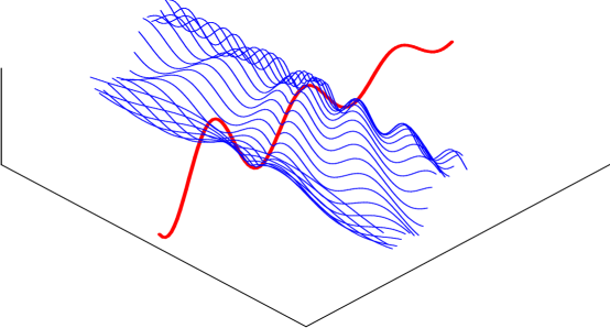
Figure 1. The extended system consists of the physical string (thick/red) coupled to an independent “hidden string” (thin/blue) at every point of dissipation. This Hamiltonian system models exactly the dissipation and dispersion in the physical string via the exchange of energy with the hidden strings.

These “hidden strings” are coupled to the physical string via a coupling function $\varsigma(x,s)$, but do not interact directly with one another. Upon “integrating out” the hidden strings, the result is an effective dynamics of the form (1.4) for the physical string, with susceptibility

(1.7) $$\chi(x,\tau)\ =\ \frac{1}{2}\int_{\mathbb{R}}\varsigma(s,x)\int_{s-\tau}^{s+\tau}\varsigma(x,r)\,\mathrm{d}r\,\mathrm{d}s.$$

Different choices of the coupling function $\varsigma(x,s)$ produce different susceptibilities $\chi(x,\tau)$, and furthermore [2, 3] any susceptibility satisfying the power dissipation condition — (1.23) below — can be obtained in this way.

Given the role of the TDD wave equation (1.4) as a phenomenological description for the interaction of the string with its environment, it is not surprising that an extended system exists which produces the effective dynamics (1.4), at least approximately. However, the main point of [2, 3], which we explain below, is that it is possible to construct explicitly an extended system which exactly reproduces (1.4). Further, using that system we can derive simple expressions for quantities like the energy and wave momentum densities for the damped string in terms of the susceptibility $\chi$.

In addition, as illustrated below, the extended system clarifies the nature and role of eigenfunctions in a TDD system by providing a natural eigenmode expansion for solutions to (1.4). In this context, an eigenfunction $\exp(-\mathrm{i}\omega t)\phi_{\omega}(x)$ is a time periodic steady state solution to (1.4). For the simple non-dissipative string (1.1), an eigenmode solves

(1.8) $$\gamma\partial_{x}^{2}\phi_{\omega}(x)\ =\ -\omega^{2}\phi_{\omega}(x),$$

which is to say it is a linear superposition of the plane waves $\exp(\pm\mathrm{i}\omega x/\sqrt{\gamma})$. For the TDD string (1.4), the dissipation induced by the dispersion in (1.6) may preclude the existence of a steady state solution without a source term. However, there is no difficulty in constructing the eigenmodes for the extended system, as it is without dissipation. We find below that the resulting eigenmode equation for $\phi_{\omega}$

(1.9) $$\gamma\partial_{x}^{2}\phi_{\omega}(x)\ =\ -\omega^{2}\left(1+\mathrm{Re}\,\widehat{\chi}(x,\omega)\right)\phi_{\omega}(x)-\mathrm{i}\omega^{2}\mathrm{Im}\,\widehat{\chi}(x,\omega)g_{\omega}(x),$$

has a source term involving an arbitrary function $g_{\omega}$, which depends on the configuration of the hidden strings. Here $\widehat{\chi}$ is the $\tau$-Fourier transform of $\chi$,

(1.10) $$\widehat{\chi}(x,\omega)\ =\ \int_{0}^{\infty}\mathrm{e}^{\mathrm{i}\omega\tau}\chi(x,\tau)\,\mathrm{d}\tau.$$

Let us now sketch the construction of the Hamiltonian extension. To start we write (1.1) as a first order system, introducing the momentum density $\pi(x,t)\ =\partial_{t}\phi(x,t)$, so that

(1.11) $$\partial_{t}\phi(x,t) =\ \pi(x,t)$$

$$\partial_{t}\pi(x,t) =\ \gamma\partial_{x}^{2}\phi(x,t)+f(x,t).$$

This first order system is Hamiltonian, with symplectic form

(1.12) $$J(\phi_{1},\pi_{1};\phi_{2},\pi_{2})\ =\ \int_{\mathbb{R}}(\phi_{1}(x)\pi_{2}(x)-\phi_{2}(x)\pi_{1}(x))\,\mathrm{d}x$$

and time dependent Hamilton function

(1.13) $$H_{f}(\phi,\pi,t)\ =\ \frac{1}{2}\int_{\mathbb{R}}\left(\pi(x)^{2}+\gamma|\partial_{x}\phi(x)|^{2}\right)\,\mathrm{d}x-\int_{\mathbb{R}}f(x,t)\phi(x)\,\mathrm{d}x.$$

As the system is non-autonomous, $H_{f}(\pi(\cdot,t),\phi(\cdot,t),t)$ is not conserved. Instead along a trajectory to (1.11), we have

(1.14) $$\frac{\mathrm{d}H_{f}}{\mathrm{d}t}\ =\ \partial_{t}H_{f}(\phi(\cdot,t),\pi(\cdot,t),t)\ =\ -\int_{\mathbb{R}}\partial_{t}f(x,t)\phi(x,t)\,\mathrm{d}x.$$

We take the internal energy of the (undamped) string to be the Hamilton function $H_{0}(\phi,\pi)$ of the system with $f\equiv 0$. Thus, using (1.14) we obtain

(1.15) $$\frac{\mathrm{d}H_{0}}{\mathrm{d}t}\ =\ \frac{\mathrm{d}H_{f}}{\mathrm{d}t}+\frac{\mathrm{d}\ }{\mathrm{d}t}\int_{\mathbb{R}}f(x,t)\phi(x,t)\,\mathrm{d}x\ =\ \int_{\mathbb{R}}f(x,t)\partial_{t}\phi(x,t)\,\mathrm{d}x.$$

In other words, the rate of work done on the system is the integral of the external force times the velocity – “power $=$ force $\times$ velocity.”

Observe that the Hamiltonian $H_{0}$ can be written

(1.16) $$H_{0}(\phi,\pi)\ =\ \frac{1}{2}\left(\|K_{\pi}\pi\|_{L^{2}(\mathbb{R})}^{2}+\|K_{\phi}\phi\|_{L^{2}(\mathbb{R})}^{2}\right)$$

where

(1.17) $$K_{\phi}\ =\ \sqrt{\gamma}\partial_{x},\quad K_{\pi}\ =\ \text{Identity}.$$

Based on this expression, we separate the equations of motion (1.11), into “material relations”

(1.18) $$f_{\phi}(x)\ =\ K_{\phi}\phi(x)\ =\ \sqrt{\gamma}\partial_{x}\phi(x)$$

(1.19) $$f_{\pi}(x)\ =\ K_{\pi}\pi(x)\ =\ \pi(x),$$

and dynamical equations,

(1.20) $$\partial_{t}\phi(x,t) =\ K_{\pi}^{\dagger}f_{\pi}(x,t)$$

$$\partial_{t}\pi(x,t) =\ -K_{\phi}^{\dagger}f_{\phi}(x,t)+f(x,t).$$

To obtain a first order TDD system leading to (1.4), we follow [2, 3] and replace the identity (1.19) with the “material relation,”

(1.21) $$f_{\pi}(x,t)+\int_{0}^{\infty}\chi(x,\tau)f_{\pi}(x,t-\tau)\,\mathrm{d}\tau\ =\ \pi(x,t),$$

but maintain (1.18) and the equations of motion (1.20), i.e.,

(1.22) $$\partial_{t}\phi(x,t) =\ f_{\pi}(x,t)$$

$$\partial_{t}\pi(x,t) =\ \gamma\partial_{x}^{2}\phi(x,t)+f(x,t).$$

(One could also introduce dispersion in the relation between $\phi$ and $f_{\phi}$, or even dispersion mixing $f_{\phi}$ and $f_{\pi}$, but for simplicity we consider here only TDD in the momentum.) The key requirements on the susceptibility $\chi$ are

1. Causality, manifest in (1.21) in that the integral on the l.h.s. depends only on the past.

2. Power dissipation, which is the requirement that for every $x$

   (1.23) $$\int_{-\infty}^{\infty}g(t)\int_{0}^{\infty}\chi(x,\tau)\partial_{t}g(t-\tau)\,\mathrm{d}\tau\,\mathrm{d}t\ \geq\ 0$$

   for an arbitrary function $g(t)$, say compactly supported.

The significance of the power dissipation condition is as follows. We suppose that the internal energy of the TDD system at time $t$ is given by

(1.24) $$H_{0}\ =\ \frac{1}{2}\int_{\mathbb{R}}\left(f_{\pi}(x,t)^{2}+\gamma\partial_{x}\phi(x,t)^{2}\right)\,\mathrm{d}x,$$

with $f_{\pi}(x,t)$ as in (1.21). Then

(1.25) $$\frac{\mathrm{d}}{\mathrm{d}t}H_{0}(t)$$

$$=\ \int_{\mathbb{R}}\Bigl{(}\gamma\partial_{x}\phi(x,t)\partial_{t}\partial_{x}\phi(x,t)\ +\ f_{\pi}(x,t)\partial_{t}f_{\pi}(x,t)\Bigr{)}\,\mathrm{d}x$$

$$=\ \int_{\mathbb{R}}\Bigl{(}\gamma\partial_{x}\phi(x,t)\partial_{x}f_{\pi}(x,t)\ +\ f_{\pi}(x,t)\partial_{t}\pi(x,t)$$

$$\quad\quad\quad-f_{\pi}(x,t)\int_{0}^{\infty}\chi(x,\tau)\partial_{t}f_{\pi}(x,t-\tau)\,\mathrm{d}\tau\Bigr{)}\,\mathrm{d}x$$

$$=\ \int_{\mathbb{R}}\Bigl{(}\gamma\partial_{x}\phi(x,t)\partial_{x}f_{\pi}(x,t)\ +\ \gamma f_{\pi}(x,t)\partial_{x}^{2}\phi(x,t)$$

$$\quad\quad\quad\ +\ f_{\pi}(x,t)f(x,t)\ -\ f_{\pi}(x,t)\int_{0}^{\infty}\chi(x,\tau)\partial_{t}f_{\pi}(x,t-\tau)\,\mathrm{d}\tau\Bigr{)}\,\mathrm{d}x$$

$$=\ \int_{\mathbb{R}}f(x,t)\partial_{t}\phi(x,t)\,\mathrm{d}x\ -\ \int_{\mathbb{R}}\left[\int_{0}^{\infty}\chi(x,\tau)\partial_{t}^{2}\phi(x,t-\tau)\,\mathrm{d}\tau\right]\partial_{t}\phi(x,t)\,\mathrm{d}x,$$

where in going from the third to the final line we have used integration by parts and the assumption that $\partial_{x}\phi$ and $f_{\pi}$ vanish at spatial infinity. The first term on the r.h.s. is the rate of work done on the system by the external force $f$. Similarly, we interpret the second term as the power loss of the dissipative force, $-\int\chi(\tau)\partial_{t}^{2}\phi(x,t-\tau)\mathrm{d}\tau$. Thus, power dissipation amounts to the requirement that, for any trajectory, the total work done by the dissipative force is negative.

Let us note that the right hand side of (1.23) is equal to

(1.26) $$\chi(x,0)\int_{-\infty}^{\infty}g(t)^{2}\,\mathrm{d}t+\int_{-\infty}^{\infty}g(t)\int_{0}^{\infty}\partial_{\tau}\chi(x,\tau)g(t-\tau)\,\mathrm{d}\tau\,\mathrm{d}t\\ =\ \int_{\mathbb{R}^{2}}\Bigl{\{}\chi(x,0)\delta(t_{1}-t_{2})+\frac{1}{2}[\partial_{\tau}\chi](x,|t_{1}-t_{2}|)\Bigr{\}}g(t_{1})g(t_{2})\,\mathrm{d}^{2}t,$$

which follows from integration by parts after noting that $\partial_{t}g(t-\tau)=-\partial_{\tau}g(t-\tau)$. Here $\delta(t)$ is the Dirac delta function. Thus the power dissipation condition is equivalent to the statement that for every $x$ the (generalized) function

(1.27) $$D_{\chi}(x,t)\ =\ \chi(x,0)\delta(t)+\frac{1}{2}[\partial_{\tau}\chi](x,|t|)$$

is positive definite in the sense of the classical Bochner’s Theorem, see [7, Theorem IX.9]. Thus, by Bochner’s Theorem, the time Fourier transform of $D_{\chi}$ is a non-negative measure,

(1.28) $$\widehat{D}_{\chi}(x,\omega)\ =\ \chi(x,0)+\frac{1}{2}\int_{-\infty}^{\infty}[\partial_{\tau}\chi](x,|t|)\mathrm{e}^{\mathrm{i}\omega t}\,\mathrm{d}t\\ =\ \chi(x,0)+\int_{0}^{\infty}\partial_{\tau}\chi(x,\tau)\cos(\omega\tau)\,\mathrm{d}\tau\\ =\ \omega\int_{0}^{\infty}\chi(x,\tau)\sin(\omega\tau)\,\mathrm{d}\tau\ =\ \omega\mathrm{Im}\widehat{\chi}(x,\omega)\ \geq\ 0.$$

Since $\chi$ is real, $\widehat{D}_{\chi}(x,\omega)$ is symmetric under $\omega\leftrightarrow-\omega$, and indeed Bochner’s Theorem shows that a symmetric measure of suitably bounded growth is non-negative if and only if it is the Fourier transform of a real positive definite distribution.

The simplest physically relevant example of a susceptibility satisfying the power dissipation condition is obtained with $\chi(x,\tau)=\alpha>0$, a positive constant. Then

(1.29) $$f_{\pi}(x,t)+\alpha\int_{0}^{\infty}f_{\pi}(x,t-\tau)\,\mathrm{d}\tau\ =\ \pi(x,t).$$

Using the equation of motion $f_{\pi}=\partial_{t}\phi$, we find that

(1.30) $$\pi(x,t) =\ \partial_{t}\phi(x,t)+\alpha\int_{0}^{\infty}\partial_{t}\phi(x,t-\tau)\,\mathrm{d}\tau$$

$$=\ \partial_{t}\phi(x,t)+\alpha\phi(x,t),$$

where we have applied the boundary condition $\lim_{t\rightarrow-\infty}\phi(x,t)=0$. Combined with the equation of motion $\partial_{t}\pi=\gamma\partial_{x}^{2}\phi+f$ we obtain

(1.31) $$\partial_{t}^{2}\phi(x,t)+\alpha\partial_{t}\phi(x,t)-\gamma\partial_{x}^{2}\phi(x,t)\ =\ f(x,t),$$

which is the dynamical equation for a driven damped string, with damping force per unit length $-\alpha\partial_{t}\phi(x,t).$ Note that $\alpha$ is dimensionally an inverse time and $1/\alpha$ is the characteristic time for the damping of oscillations.

A more realistic model for damping is obtained by supposing $\chi(x,\tau)$ to be a non-trivial function of $\tau$ as in (1.21). To allow for damping restricted to only a part of the string, we suppose that $\chi$ depends on $x$ as well. For instance, we could take the Debye susceptibility

(1.32) $$\chi(x,\tau)\ =\alpha(x)\mathrm{e}^{-\nu(x)\tau},$$

with $\alpha(x)\geq 0$ and $\nu(x)\geq 0$ non-negative functions of $x$. This results in the following integral-differential equation for $\phi$

(1.33) $$\partial_{t}^{2}\phi(x,t)+\alpha(x)\int_{0}^{\infty}\mathrm{e}^{-\nu(x)\tau}\partial_{t}^{2}\phi(x,t-\tau)\,\mathrm{d}\tau-\gamma\partial_{x}^{2}\phi(x,t)\ =\ f(x,t),$$

or after integration by parts

(1.34) $$\partial_{t}^{2}\phi(x,t)+\alpha(x)\partial_{t}\phi(x,t)-\alpha(x)\nu(x)\phi(x,t)\\ +\alpha(x)\nu(x)^{2}\int_{0}^{\infty}\mathrm{e}^{-\nu(x)\tau}\phi(x,t-\tau)\,\mathrm{d}\tau-\gamma\partial_{x}^{2}\phi(x,t)\ =\ f(x,t).$$

Then

(1.35) $$\widehat{D}_{\chi}(x,\omega)\ =\ \alpha(x)\int_{0}^{\infty}\mathrm{e}^{-\nu(x)\tau}\omega\sin(\omega\tau)\,\mathrm{d}\tau\ =\ \alpha(x)\frac{\omega^{2}}{\nu(x)^{2}+\omega^{2}}\ \geq\ 0,$$

so the Debye susceptibility satisfies the power dissipation condition.

The results of [2, 3] show that under the above conditions it is possible to find a coupling function $\varsigma(x,s)$, $s\in\mathbb{R}$, such that solutions to the TDD equations are generated by solutions to the following extended system

(1.36) $$\partial_{t}\phi(x,t) =\ f_{\pi}(x,t)$$

$$\partial_{t}\pi(x,t) =\ \gamma\partial_{x}^{2}\phi(x,t)+f(x,t)$$

$$\partial_{t}\psi(x,s,t) =\ \theta(x,s,t)$$

$$\partial_{t}\theta(x,s,t) =\ \partial_{s}^{2}\psi(x,s,t)+\varsigma(x,s)f_{\pi}(x,t),$$

with

(1.37) $$f_{\pi}(x,t)\ =\ \pi(x,t)-\int_{-\infty}^{\infty}\varsigma(x,s)\psi(x,s,t)\,\mathrm{d}s.$$

That is, given a solution $(\phi,\pi,\psi,\theta)$ to (1.36), at rest at $t=-\infty$ and with $f_{\pi}$ given by (1.37), the first two coordinates $(\phi,\pi)$ obey (1.22) with $f_{\pi}$ given by (1.21), and conversely any solution to (1.21, 1.22) with the string at rest at $t=-\infty$ arises in this way. Note that for each fixed $x$ the additional variables $\theta,\psi$ may be interpreted as describing the oscillations of a “hidden string” with coordinate $s$, displacement $\psi(x,s,t)$, momentum $\theta(x,s,t)$ and driven by external force $\varsigma(x,s)f_{\pi}(x,t)$. Thus (1.36) is precisely the system of coupled strings described above and illustrated in Figure 1.

The extended system, consisting of the physical and hidden strings is Hamiltonian with symplectic form

(1.38) $$\mathcal{J}(\phi_{1},\pi_{1},\psi_{1},\theta_{1};\phi_{2},\pi_{2},\psi_{2},\theta_{2})\ =\ \int_{\mathbb{R}}\left\{\phi_{1}(x)\pi_{2}(x)-\phi_{2}(x)\pi_{1}(x)\right\}\mathrm{d}x\\ +\int_{\mathbb{R}^{2}}\left\{\psi_{1}(x,s)\theta_{2}(x,s)-\psi_{2}(x,s)\theta_{1}(x,s)\right\}\mathrm{d}s\,\mathrm{d}x$$

and Hamilton function

(1.39) $$\mathcal{H}_{f}(\phi,\pi,\psi,\theta,t)\ =\ \frac{1}{2}\int_{\mathbb{R}}\left\{f_{\pi}(x)^{2}+\gamma(\partial_{x}\phi(x))^{2}\right\}\mathrm{d}x-\int_{\mathbb{R}}f(x,t)\phi(x)\,\mathrm{d}x\\ +\frac{1}{2}\int_{\mathbb{R}^{2}}\left\{\theta(x,s)^{2}+(\partial_{s}\psi(x,s))^{2}\right\}\mathrm{d}s\,\mathrm{d}x,$$

where $f_{\pi}$ is given by (1.37), that is $f_{\pi}(x)\ =\ \pi(x)-\int\varsigma(x,s)\psi(x,s)\,\mathrm{d}s$.

The dynamical equation for an excitation of the hidden string at $x$ is a driven wave equation

(1.40) $$\partial_{t}^{2}\psi(x,s,t)\ =\ \partial_{s}^{2}\psi(x,s,t)+\varsigma(x,s)f_{\pi}(x,t).$$

The solution to (1.40) with the hidden string at rest at $t=-\infty$ is easily written down, see (1.3):

(1.41) $$\psi(x,s,t)\ =\ \frac{1}{2}\int_{0}^{\infty}\int_{s-\tau}^{s+\tau}\varsigma(x,r)\,\mathrm{d}r\,f_{\pi}(x,t-\tau)\,\mathrm{d}\tau.$$

Thus

(1.42) $$\int_{\mathbb{R}}\varsigma(x,s)\psi(x,s,t)\,\mathrm{d}s\\ =\ \int_{0}^{\infty}\left[\frac{1}{2}\int_{\mathbb{R}}\varsigma(x,s)\int_{s-\tau}^{s+\tau}\varsigma(x,r)\,\mathrm{d}r\,\mathrm{d}s\right]f_{\pi}(x,t-\tau)\,\mathrm{d}\tau.$$

Comparing (1.21) and (1.37) we see that for the extension to reproduce the TDD system upon elimination of $\psi$ and $\theta$ it is necessary and sufficient that the coupling $\varsigma(x,s)$ satisfy (1.7), that is

(1.43) $$\chi(x,\tau)\ =\ \frac{1}{2}\int_{\mathbb{R}}\varsigma(s,x)\int_{s-\tau}^{s+\tau}\varsigma(x,r)\,\mathrm{d}r\,\mathrm{d}s.$$

The existence of such a function, which is unique under a natural symmetry assumption, is guaranteed by the power dissipation condition [2, 3].

Indeed, if we let $\widehat{\varsigma}(x,\sigma)$ denote the $s$-Fourier transform of $\varsigma$,

(1.44) $$\widehat{\varsigma}(x,\sigma)\ =\ \int_{\mathbb{R}}\varsigma(x,s)\mathrm{e}^{\mathrm{i}\sigma s}\,\mathrm{d}s,$$

then (1.43) is equivalent to

(1.45) $$\widehat{D}_{\chi}(x,\omega)\ =\ \widehat{\varsigma}(x,\omega)\widehat{\varsigma}(x,-\omega),$$

so it suffices to take [2]

(1.46) $$\widehat{\varsigma}(x,\sigma)\ =\ \sqrt{2\widehat{D}_{\chi}(x,\sigma)}.$$

Furthermore, this choice of $\widehat{\varsigma}(x,\sigma)$ is unique if we ask further that $\widehat{\varsigma}(x,\sigma)\geq 0$ and that $\sigma\mapsto\widehat{\varsigma}(x,\sigma)$ be symmetric. Then,

(1.47) $$\varsigma(x,s)\ =\ \frac{1}{2\pi}\int_{\mathbb{R}}\sqrt{2\widehat{D}_{\chi}(x,\sigma)}\mathrm{e}^{-\mathrm{i}\sigma s}\,\mathrm{d}\sigma\ =\ \frac{1}{2\pi}\int_{\mathbb{R}}\sqrt{2\widehat{D}_{\chi}(x,\sigma)}\cos(\sigma s)\,\mathrm{d}\sigma,$$

is real, symmetric, and positive definite.

For example, in view of (1.28), (1.35), and (1.47), the following coupling produces the Debye susceptibility,

(1.48) $$\varsigma(x,s)\ =\ \sqrt{2\alpha(x)}\partial_{s}\Psi(\nu(x)s).$$

where

(1.49) $$\Psi(s)\ =\ \frac{1}{2\pi\mathrm{i}}\int_{-\infty}^{\infty}\frac{1}{\omega}\sqrt{\frac{\omega^{2}}{1+\omega^{2}}}\mathrm{e}^{\mathrm{i}\omega s}\,\mathrm{d}\omega\\ =\ \frac{s}{|s|}\frac{1}{\pi}\int_{0}^{1}\frac{1}{\sqrt{1-u^{2}}}\mathrm{e}^{-u|s|}\,\mathrm{d}u\ =\ \frac{s}{|s|}\frac{1}{\pi}\int_{0}^{\frac{\pi}{2}}\mathrm{e}^{-|s|\sin(\phi)}\,\mathrm{d}\phi.$$

That is,

(1.50) $$\varsigma(x,s)\ =\ \sqrt{2\alpha(x)}\left(\delta(s)-\frac{\nu(x)}{\pi}\int_{0}^{\frac{\pi}{2}}\sin(\phi)\mathrm{e}^{-\nu(x)|s|\sin(\phi)}\,\mathrm{d}\phi\right).$$

2. Local energy and momentum conservation in the extended system

We interpret the Hamiltonian $\mathcal{H}_{0}$ with $f\equiv 0$ as the internal energy of the damped string system consisting of the coupled physical and hidden strings. We have conservation of energy in the extended system, in the form

(2.1) $$\frac{\mathrm{d}\ }{\mathrm{d}t}\mathcal{H}_{0}\ =\ \int_{\mathbb{R}}f(x,t)\partial_{t}\phi(x,t)\,\mathrm{d}x,$$

i.e., the rate of change of $\mathcal{H}_{0}$ is the rate of work done on the system by the external force.

A significant advantage of working with the extended system is a transparent interpretation of the energy of the dissipative string as a sum of contributions from the physical and hidden strings. That is, it is natural to break the $\mathcal{H}_{0}$ into two pieces

(2.2) $$\mathcal{H}_{0}(\phi,\pi,\psi,\theta,t)\ =\ H_{0}(\phi,\pi,\psi)+H_{hs}(\psi,\theta),$$

the energy of the physical string and hidden strings respectively,

(2.3) $$H_{0}(\phi,\pi,\psi)\ =\ \frac{1}{2}\int_{\mathbb{R}}\left\{f_{\pi}(x)^{2}+\gamma(\partial_{x}\phi(x))^{2}\right\}\mathrm{d}x$$

(2.4) $$H_{hs}(\psi,\theta)\ =\ \frac{1}{2}\int_{\mathbb{R}^{2}}\left\{\theta(x,s)^{2}+(\partial_{s}\psi(x,s))^{2}\right\}\mathrm{d}s\mathrm{d}x,$$

with $f_{\pi}$ given by (1.37).

The internal energy $\mathcal{H}_{0}$ can be written as the integral of a local energy density

(2.5) $$\mathcal{E}(x,t)\ =\ E_{0}(x,t)+E_{hs}(x,t)$$

with

(2.6) $$E_{0}(x,t) =\ \frac{1}{2}\left\{(\partial_{t}\phi(x,t))^{2}+\gamma(\partial_{x}\phi(x,t))^{2}\right\}$$

$$E_{hs}(x,t) =\ \frac{1}{2}\int_{\mathbb{R}}\left\{(\partial_{t}\psi(x,s,t))^{2}+(\partial_{s}\psi(x,s,t))^{2}\right\}\mathrm{d}s.$$

The energy conservation law (2.1) has the following local expression

(2.7) $$\partial_{t}\mathcal{E}(x,t)+\partial_{x}J(x,t)\ =\ f(x,t)\partial_{t}\phi(x,t)$$

with the energy current

(2.8) $$J(x,t)\ =\ -\gamma f_{\pi}(x,t)\partial_{x}\phi(x,t)\ =\ -\gamma\partial_{t}\phi(x,t)\partial_{x}\phi(x,t).$$

It is interesting to compute the time derivatives of $E_{0}$ and $E_{hs}$ alone:

(2.9) $$\partial_{t}E_{0}(x,t)+\partial_{x}J(x,t)\ =\ f(x,t)\partial_{t}\phi(x,t)-\partial_{t}\Delta(x,t)\partial_{t}\phi(x,t)$$

(2.10) $$\partial_{t}E_{hs}(x,t)\ =\ \partial_{t}\Delta(x,t)\partial_{t}\phi(x,t)$$

with

(2.11) $$\Delta(x,t)\ =\ \pi(x,t)-f_{\pi}(x,t)\\ =\ \int_{\mathbb{R}}\varsigma(x,s)\psi(x,s,t)\,\mathrm{d}s\ =\ \int_{0}^{\infty}\chi(x,\tau)\partial_{t}\phi(x,t-\tau)\,\mathrm{d}\tau,$$

where we have used (1.42). The first of these equations (2.9) is simply the local version of the energy law for the TDD string (1.25). From the second (2.10), we see that the energy of the hidden strings, which is the energy lost to dissipation up to time $t$, is

(2.12) $$E_{hs}(x,t) =\ \int_{-\infty}^{t}\partial_{t^{\prime}}\phi(x,t^{\prime})\int_{0}^{\infty}\chi(x,\tau)\partial_{t^{\prime}}^{2}\phi(x,t^{\prime}-\tau)\,\mathrm{d}\tau\,\mathrm{d}t^{\prime}.$$

$$=\ \int_{-\infty}^{t}\int_{-\infty}^{t}D_{\chi}(x,t_{1}-t_{2})\partial_{t_{1}}\phi(x,t_{1})\partial_{t_{2}}\phi(x,t_{2})\,\mathrm{d}t_{1}\,\mathrm{d}t_{2}.$$

If the susceptibility $\chi$ — and hence the coupling $\varsigma$ — is independent of $x$, then the extended system is invariant under spatial translations. Associated to this symmetry is a local conservation law

(2.13) $$\partial_{t}p(x,t)+\partial_{x}T(x,t)\ =\ -f(x,t)\partial_{x}\phi(x,t),$$

for the wave momentum density

(2.14) $$p(x,t) =\ -\pi(x,t)\partial_{x}\phi(x,t)-\int_{\mathbb{R}}\theta(x,s,t)\partial_{x}\psi(x,s,t)\mathrm{d}s$$

$$=\ -\left\{\partial_{t}\phi(x,t)+\Delta(x,t)\right\}\partial_{x}\phi(x,t)-\int_{\mathbb{R}}\partial_{t}\psi(x,s,t)\partial_{x}\psi(x,s,t)\,\mathrm{d}s,$$

with wave momentum flux, called stress,

(2.15) $$T(x,t)\ =\ E_{0}(x,t)+\Delta(x,t)\partial_{t}\phi(x,t)\\ +\int\left\{(\partial_{t}\psi(x,s,t))^{2}-(\partial_{s}\psi(x,s,t))^{2}\right\}\mathrm{d}s.$$

When the driving force vanishes, $f=0$, the total wave momentum

(2.16) $$P\ =\ \int_{\mathbb{R}}p(x,t)\,\mathrm{d}x$$

is a conserved quantity.

The wave momentum density $p=p_{0}+p_{hs}$ is again a sum of contributions

(2.17) $$p_{0}(x,t)\ =\ -\left\{\partial_{t}\phi(x,t)+\Delta(x,t)\right\}\partial_{x}\phi(x,t)$$

(2.18) $$p_{hs}(x,t)\ =\ -\int_{\mathbb{R}}\partial_{t}\psi(x,s,t)\partial_{x}\psi(x,s,t)\,\mathrm{d}s$$

from the physical and hidden strings. Likewise we separate the stress

(2.19) $$T(x,t)\ =\ T_{0}(x,t)+T_{hs}(x,t)$$

into two pieces,

(2.20) $$T_{0}(x,t)\ =\ E_{0}(x,t)+\Delta(x,t)\partial_{t}\phi(x,t)$$

(2.21) $$T_{hs}(x,t)\ =\ \frac{1}{2}\int\left\{(\partial_{t}\psi(x,s,t))^{2}-(\partial_{s}\psi(x,s,t))^{2}\right\}\mathrm{d}s.$$

Then

(2.22) $$\partial_{t}p_{0}(x,t)+\partial_{x}T_{0}(x,t)\ =\ -f(x,t)\partial_{x}\phi(x,t)+\partial_{x}\Delta(x,t)\partial_{t}\phi(x,t)$$

(2.23) $$\partial_{t}p_{hs}(x,t)+\partial_{x}T_{hs}(x,t)\ =\ -\partial_{x}\Delta(x,t)\partial_{t}\phi(x,t).$$

When we study eigenfunctions below, it will be convenient to work with complex valued solutions. In the above expressions, terms which are quadratic in the field variables should be modified in the complex case by the replacement $ab\rightarrow\mathrm{Re}\,\overline{a}b$. That is

(2.24) $$E_{0}(x,t) =\ \frac{1}{2}\left\{|\partial_{t}\phi(x,t)|^{2}+\gamma|\partial_{x}\phi(x,t)|^{2}\right\}$$

$$E_{hs}(x,t) =\ \frac{1}{2}\int_{\mathbb{R}}\left\{|\partial_{t}\psi(x,s,t)|^{2}+|\partial_{s}\psi(x,s,t)|^{2}\right\}\mathrm{d}s$$

$$J(x,t) =\ -\gamma\mathrm{Re}\,\overline{\partial_{t}\phi(x,t)}\partial_{x}\phi(x,t)$$

$$p_{0}(x,t) =\ -\mathrm{Re}\,\overline{\partial_{t}\phi(x,t)}\partial_{x}\phi(x,t)-\mathrm{Re}\,\overline{\Delta(x,t)}\partial_{x}\phi(x,t),$$

etc.

3. The eigenfunction equation

It is useful and interesting to study steady state solutions to the extended system (1.36), for example solutions which are periodic in time $\mathrm{e}^{-\mathrm{i}\omega t}(\phi_{\omega}(x),\pi_{\omega}(x),$ $\psi_{\omega}(x,s),\theta_{\omega}(x,s))$. We refer to the spatial component $\Phi_{\omega}(x,s)=(\phi_{\omega}(x),\pi_{\omega}(x),$ $\psi_{\omega}(x,s),\theta_{\omega}(x,s))$ of such a time periodic solution as an eigenfunction for the linear system (1.36) with eigenvalue $\omega$. Thus an eigenfunction satisfies

(3.1) $$-\mathrm{i}\omega\phi_{\omega}(x) =\ f_{\pi}(x)$$

$$-\mathrm{i}\omega\pi_{\omega}(x) =\ \gamma\partial_{x}^{2}\phi_{\omega}(x)$$

$$-\mathrm{i}\omega\psi_{\omega}(x,s) =\ \theta_{\omega}(x,s)$$

$$-\mathrm{i}\omega\theta_{\omega}(x,s) =\ \partial_{s}^{2}\psi_{\omega}(x,s)+\varsigma(x,s)f_{\pi}(x),$$

with

(3.2) $$f_{\pi}(x)+\int_{\mathbb{R}}\varsigma(x,s)\psi_{\omega}(x,s)\,\mathrm{d}s-\pi_{\omega}(x)\ =\ 0.$$

We see that the displacement of the hidden string at position $x$ satisfies

(3.3) $$-\partial_{s}^{2}\psi_{\omega}(x,s)-\omega^{2}\psi_{\omega}(x,s)\ =\ -\mathrm{i}\omega\varsigma(x,s)\phi_{\omega}(x),$$

so

(3.4) $$\psi_{\omega}(x,s)\\ \begin{aligned} &=\ a(x)\cos(\omega s)+b(x)\sin(\omega s)-\frac{\mathrm{i}\omega\phi_{\omega}(x)}{2\pi}\mathrm{P.V.}\int_{-\infty}^{\infty}\mathrm{e}^{-\mathrm{i}\sigma s}\frac{1}{\sigma^{2}-\omega^{2}}\widehat{\varsigma}(x,\sigma)\,\mathrm{d}\sigma\\ &=\ a(x)\cos(\omega s)+b(x)\sin(\omega s)+\frac{\mathrm{i}\phi_{\omega}(x)}{2}\int_{-\infty}^{\infty}\sin(\omega|s^{\prime}-s|)\varsigma(x,s^{\prime})\,\mathrm{d}s^{\prime},\end{aligned}$$

with $a(x)$ and $b(x)$ undetermined functions of $x$. Here, $\mathrm{P.V.}$ denotes the “principle value” integral,

(3.5) $$\mathrm{P.V.}\int_{-\infty}^{\infty}\mathrm{e}^{-\mathrm{i}\sigma s}\frac{1}{\sigma^{2}-\omega^{2}}\widehat{\varsigma}(x,\sigma)\mathrm{d}\sigma\\ \begin{aligned} &=\ \lim_{\delta\downarrow 0}\int_{\{\sigma\ :\ |\sigma^{2}-\omega^{2}|\geq\delta\}}\mathrm{e}^{-\mathrm{i}\sigma s}\frac{1}{\sigma^{2}-\omega^{2}}\widehat{\varsigma}(x,\sigma)\,\mathrm{d}\sigma\\ &=\ \lim_{\delta\downarrow 0}\frac{1}{2}\int_{\mathbb{R}}\mathrm{e}^{-\mathrm{i}\sigma s}\left[\frac{1}{\sigma^{2}-(\omega+\mathrm{i}\delta)^{2}}+\frac{1}{\sigma^{2}-(\omega-\mathrm{i}\delta)^{2}}\right]\widehat{\varsigma}(x,\sigma)\,\mathrm{d}\sigma.\end{aligned}$$

By (3.4), we see that

(3.6) $$\int_{\mathbb{R}}\varsigma(x,s)\psi_{\omega}(x,s)\mathrm{d}s\ =\ a(x)\widehat{\varsigma}(x,\omega)\\ -\ \frac{\phi_{\omega}(x)}{2\pi}\mathrm{P.V.}\int_{-\infty}^{\infty}\frac{\mathrm{i}\omega}{\sigma^{2}-\omega^{2}}\widehat{\varsigma}(x,\sigma)\widehat{\varsigma}(x,-\sigma)\,\mathrm{d}\sigma.$$

Recalling (1.45), that $\widehat{\varsigma}(x,\sigma)\widehat{\varsigma}(x,-\sigma)=\widehat{D}_{\chi}(x,\sigma)=2\sigma\mathrm{Im}\,\widehat{\chi}(x,\sigma)$, we see that the final term on the r.h.s. can be expressed

(3.7) $$-\frac{\phi_{\omega}(x)}{2\pi}\mathrm{P.V.}\int_{-\infty}^{\infty}\frac{2\mathrm{i}\omega}{\sigma^{2}-\omega^{2}}\sigma\mathrm{Im}\,\widehat{\chi}(x,\sigma)\,\mathrm{d}\sigma\\ \begin{aligned} &=\ -\frac{\mathrm{i}\phi_{\omega}(x)}{2\pi}\mathrm{P.V.}\int_{-\infty}^{\infty}\left\{\frac{1}{\sigma-\omega}+\frac{1}{-\sigma-\omega}\right\}\sigma\mathrm{Im}\,\widehat{\chi}(x,\sigma)\,\mathrm{d}\sigma\\ &=\ -\mathrm{i}\omega\mathrm{Re}\,\widehat{\chi}(x,\omega)\phi_{\omega}(x),\end{aligned}$$

where we have used the symmetry $\sigma\mathrm{Im}\,\widehat{\chi}(x,\sigma)=-\sigma\mathrm{Im}\,\widehat{\chi}(x,-\sigma)$ and the “Kramers-Krönig relation”

(3.8) $$\omega\mathrm{Re}\,\widehat{\chi}(x,\omega)\ =\ \mathrm{P.V.}\frac{1}{\pi}\int_{-\infty}^{\infty}\frac{1}{\sigma-\omega}\sigma\mathrm{Im}\,\widehat{\chi}(x,\sigma)\,\mathrm{d}\sigma.$$

Plugging this result into (3.2) and combining the first two equations of (3.1) we find that the string displacement $\phi$ solves the following elliptic problem

(3.9) $$\gamma\partial_{x}^{2}\phi_{\omega}(x)\ =\ -\omega^{2}(1+\mathrm{Re}\widehat{\chi}(x,\omega))\phi_{\omega}(x)-\mathrm{i}\omega a(x)\widehat{\varsigma}(x,\omega).$$

In analyzing (3.9) we should distinguish two cases:

1. $\widehat{\varsigma}(x,\omega)=0$ for all $x$.

2. $\widehat{\varsigma}(x,\omega)$ non zero for $x$ in an open set.

In the first case, which is non-generic, the medium described by the hidden strings is not absorbing at the given frequency $\omega$, that is $\widehat{\chi}(x,\omega)$ is real for every $x$. Thus (3.9) is a very strong restriction on $\phi_{\omega}$, namely that it should satisfy the Schrödinger equation

(3.10) $$(-\gamma\partial_{x}^{2}+V(x))\phi_{\omega}(x)=\lambda\phi_{\omega}(x),$$

with potential $V(x)=-\omega^{2}\widehat{\chi}(x,\omega)$ and spectral parameter $\lambda=\omega^{2}$. In the second case, the physical string displacement may be decomposed as follows

(3.11) $$\phi_{\omega}(x)\ =\ \phi_{\omega}^{(1)}(x)+\phi_{\omega}^{(2)}(x),$$

where $\phi_{\omega}^{(1)}(x)$ is any solution to the non-dissipative eigenfunction equation

(3.12) $$\gamma\partial_{x}^{2}\phi_{\omega}^{(1)}(x)\ =\ -\omega^{2}(1+\mathrm{Re}\,\widehat{\chi}(x,\omega))\phi_{\omega}^{(1)}(x),$$

and $\phi_{\omega}^{(2)}$ is an arbitrary function with support in $\{x\ :\ \widehat{\varsigma}(x,\omega)\neq 0\}$. Indeed, given $\phi_{\omega}^{(1)}$ and $\phi_{\omega}^{(2)}$ we need only choose $a$ to be

(3.13) $$a(x)\ =\ \mathrm{i}\frac{\gamma\partial_{x}^{2}\phi_{\omega}^{(2)}(x)+\omega^{2}(1+\mathrm{Re}\,\widehat{\chi}(x,\omega))\phi_{\omega}^{(2)}(x)}{\omega\widehat{\varsigma}(x,\omega)}$$

to obtain a solution to (3.9).

Thus, the physical string displacement for an eigenmode $\phi_{\omega}(x)$ may be chosen arbitrarily within that part of the string which is absorbing at the given frequency $\omega$. We want to emphasize the significance of this fact, since the formal eigenvalue problem

(3.14) $$\gamma\partial_{x}^{2}\phi_{\omega}(x)\ =\ -\omega^{2}(1+\widehat{\chi}(x,\omega))\phi_{\omega}(x)$$

does not allow for such arbitrariness in the choice of $\phi_{\omega}(x)$. The resolution to this apparent contradiction lies in recognizing that a TDD system is an open part of a larger conservative Hamiltonian system. It is only for the extended Hamiltonian system that the eigenmodes $\Phi_{\omega}$ are unambiguously defined with $e^{\mathrm{i}\omega t}\Phi_{\omega}$ a stationary solution to the canonical Hamiltonian evolution equation. The “legitimate” eigenmodes for the original TDD string consist of projections $\phi_{\omega}$ of the eigenmodes $\Phi_{\omega}$ onto the subspace of the physical string. Thus a TDD string, being an open system has as many eigenmodes, i.e stationary solutions, as its the minimal conservative extension, introduced and described in [1, 2, 3]. In particular, a finite-dimensional TDD system typically has infinitely many stationary solutions and, hence, infinitely many eigenmodes. Another view on the construction of eigenmodes follows.

The eigenfunctions written down above, involving as they do arbitrary excitations of the hidden strings, may not be relevant to the dynamics (1.36) with the external force acting on the physical string. Indeed, note that the effective equation (3.9) for $\phi_{\omega}$ does not depend on the term $b(x)\sin(\omega s)$ appearing in (3.4). We shall see that eigenmodes with $b(x)\neq 0$ are not needed in the expansion of a general solution to (1.36) with a compactly supported external force. Essentially this is due to the fact that the configuration of the hidden strings remains symmetric throughout the evolution (1.36).

To proceed, it is convenient to introduce the Fourier-Laplace transform

(3.15) $$\widetilde{h}(\zeta)\ =\ \int_{\mathbb{R}}\mathrm{e}^{\mathrm{i}\zeta t}h(t)\,\mathrm{d}t,$$

defined for

1. $\zeta\in\mathbb{C}$ if $h\rightarrow 0$ super exponentially fast as $|t|\rightarrow\infty$, for instance if $h$ is compactly supported in time.

2. $\mathrm{Im}\zeta>0$ if $h\rightarrow 0$ super exponentially fast as $t\rightarrow-\infty$.

3. $\mathrm{Im}\zeta<0$ if $h\rightarrow 0$ super exponentially fast as $t\rightarrow\infty$.

Taking the Fourier-Laplace transform of (1.36) results in the following equations

(3.16) $$-\mathrm{i}\zeta\widetilde{\phi}(x,\zeta) =\ \widetilde{f}_{\pi}(x,\zeta)$$

$$-\mathrm{i}\zeta\widetilde{\pi}(x,\zeta) =\ \gamma\partial_{x}^{2}\widetilde{\phi}(x,\zeta)+\widetilde{f}(x,\zeta)$$

$$-\mathrm{i}\zeta\widetilde{\psi}(x,s,\zeta) =\ \widetilde{\theta}(x,s,\zeta)$$

$$-\mathrm{i}\zeta\widetilde{\theta}(x,s,\zeta) =\ \partial_{s}^{2}\widetilde{\psi}(x,s,\zeta)+\varsigma(x,s)\widetilde{f}_{\pi}(x,\zeta),$$

with

(3.17) $$\widetilde{f}_{\pi}(x,\zeta)\ =\ \widetilde{\pi}(x,\zeta)-\int_{-\infty}^{\infty}\varsigma(x,s)\widetilde{\psi}(x,s,\zeta)\,\mathrm{d}s.$$

Due to our consideration of solutions with the strings at rest at $t=-\infty$, we expect the quantities in (3.16) to be well defined only for $\mathrm{Im}\,\zeta>0$. However, if the driving force is compactly supported in time then $\widetilde{f}(x,\zeta)$ is defined for all $\zeta\in\mathbb{C}$, and we may extend $\widetilde{\phi}(x,\zeta)$ to $\zeta\in\mathbb{C}\setminus\mathbb{R}$ by solving (3.16). Following the eigenfunction analysis, we obtain, with $\varepsilon=$ sign of $\mathrm{Im}\zeta$,

(3.18) $$\widetilde{\psi}(x,s,\zeta)\ =\ -\frac{\mathrm{i}\zeta\widetilde{\phi}(x,\zeta)}{2\pi}\int_{-\infty}^{\infty}\mathrm{e}^{-\mathrm{i}\sigma s}\frac{1}{\sigma^{2}-\zeta^{2}}\widehat{\varsigma}(x,\sigma)\,\mathrm{d}\sigma$$

$$=\ \varepsilon\frac{\widetilde{\phi}(x,\zeta)}{2}\int_{-\infty}^{\infty}\mathrm{e}^{\mathrm{i}\varepsilon\zeta|s^{\prime}-s|}\varsigma(s^{\prime},x)\,\mathrm{d}s^{\prime},$$

(3.19) $$\gamma\partial_{x}^{2}\widetilde{\phi}(x,\zeta)\ =\ -\zeta^{2}(1+\widehat{\chi}(x,\varepsilon\zeta))\widetilde{\phi}(x,\zeta)+\widetilde{f}(x,\zeta),$$

where $\widehat{\chi}(x,\zeta)$ is defined for $\mathrm{Im}\,\zeta>0$ as

(3.20) $$\widehat{\chi}(x,\zeta)\ =\ \int_{0}^{\infty}\mathrm{e}^{\mathrm{i}\tau\zeta}\chi(x,\tau)\,\mathrm{d}\tau.$$

For a function $h$ vanishing at $+\infty$ or $-\infty$ we have the Fourier inversion formula

(3.21) $$h(t)\ =\ \frac{1}{2\pi}\int_{\mathbb{R}}\mathrm{e}^{-\mathrm{i}\omega t\mp\mathrm{\eta}t}\widetilde{h}(\omega\mp\mathrm{i}\eta)\,\mathrm{d}\omega,\quad\Bigl{(}\lim_{t=\pm\infty}h(t)=0\Bigr{)},$$

with $\eta>0$ arbitrary. Inverting the solution to (3.16) with $\eta>0$ or $<0$ produces distinct solutions to (1.36): for $\eta>0$ we obtain the desired causal solution with the strings at rest at $t=-\infty$, while for $\eta<0$ we obtain the anti-causal solution with the strings at rest at $t=+\infty$.

In a certain sense we are only interested in the causal solution to (1.36) and thus to the solution to (3.16) only for $\zeta$ in the upper half plane. However, since (3.16) involves a source term, this solution, often called the resolvent, is not directly expressed as a superposition of eigenfunctions. However, there is a general procedure for decomposing the solution to (3.16) into a superposition of eigenfunctions. Namely for $\omega\in\mathbb{R}$ we define

(3.22) $$\left(\phi_{\omega}(x),\pi_{\omega}(x),\psi_{\omega}(x,s),\theta_{\omega}(x,s)\right)\\ =\ \lim_{\delta\rightarrow 0}\left(\widetilde{\phi}(x,\omega+\mathrm{i}\delta)-\widetilde{\phi}(x,\omega-\mathrm{i}\delta),\widetilde{\pi}(x,\omega+\mathrm{i}\delta)-\widetilde{\pi}(x,\omega-\mathrm{i}\delta),\right.\\ \left.\widetilde{\psi}(x,s,\omega+\mathrm{i}\delta)-\widetilde{\psi}(x,s,\omega-\mathrm{i}\delta),\widetilde{\theta}(x,s,\omega+\mathrm{i}\delta)-\widetilde{\phi}(x,s,\omega-\mathrm{i}\delta)\right).$$

Since $\widetilde{f}(x,\zeta)$ is continuous at each $\zeta=\omega\in\mathbb{R}$, it follows from (3.16) that $(\phi_{\omega},\pi_{\omega},$ $\psi_{\omega},\theta_{\omega})$ is an eigenfunction for each $\omega$. To recover the resolvent for $\zeta$ in the upper half plane from the eigenfunctions (3.22), suppose that the external force is supported in the set $\{t\ :\ t>t_{0}\}$. Then

(3.23) $$|\widetilde{f}(x,\zeta)|\ \leq\ C\ \mathrm{e}^{-\mathrm{Im}\,\zeta t_{0}},\quad(\mathrm{Im}\,\zeta>0).$$

Thus $\exp(-\mathrm{i}\zeta t_{0})f(x,\zeta)$ is bounded in the upper half plane, and by analyticity we have,

(3.24) $$\left(\widetilde{\phi}(x,\zeta),\widetilde{\pi}(x,\zeta),\widetilde{\psi}(x,s,\zeta),\widetilde{\theta}(x,s,\zeta)\right)\\ =\ \frac{1}{2\pi\mathrm{i}}\int_{\mathbb{R}}\frac{\mathrm{e}^{\mathrm{i}(\zeta-\omega)t_{0}}}{\omega-\zeta}\left(\phi_{\omega}(x),\pi_{\omega}(x),\psi_{\omega}(x,s),\theta_{\omega}(x,s)\right)\,\mathrm{d}\omega,\quad(\mathrm{Im}\,\zeta>0)$$

expressing the solution to (3.16) as a superposition of eigenfunctions. (There is a similar formula for the advanced solution with $\mathrm{Im}\,\zeta<0$, involving an upper bound $t_{1}$ on the support of the external force.)

Now let us fix $\omega$ and suppose that we have an eigenfunction of the form (3.22). Then by (3.18) and (3.19),

(3.25) $$\psi_{\omega}(x,s)\ =\ \frac{\mathrm{i}\phi_{\omega}(x)}{2}\int_{-\infty}^{\infty}\sin(\omega|s^{\prime}-s|)\varsigma(x,s^{\prime})\,\mathrm{d}s^{\prime}+\frac{g_{\omega}(x)}{2}\cos(\omega s)\widehat{\varsigma}(x,\omega)$$

(3.26) $$\gamma\partial_{x}^{2}\phi_{\omega}(x)\ =\ -\omega^{2}(1+\mathrm{Re}\,\widehat{\chi}(x,\omega))\phi_{\omega}(x)-\mathrm{i}\omega^{2}\mathrm{Im}\,\widehat{\chi}(x,\omega)g_{\omega}(x),$$

with

(3.27) $$g_{\omega}(x)\ =\ \lim_{\delta\rightarrow 0}\left\{\widetilde{\phi}(x,\omega+\mathrm{i}\delta)+\widetilde{\phi}(x,\omega-\mathrm{i}\delta)\right\}.$$

In other words, the eigenfunctions which appear in the expansion (3.24) are of the form (3.9) with $b(x)=0$. We refer to such eigenfunctions as spectral eigenfunctions. By (3.24), the spectral eigenfunctions form a complete set for the description of the dynamics of the extended system (1.36). Thus, the freedom to choose $g_{\omega}$ in (3.26) provides us with a rich enough family of solutions to describe the dynamics of the TDD string.

Note that for $\zeta=\omega\in\mathbb{R}$, a solution to (3.16) satisfies the eigenmode equation away from the spatial support of the driving force. Thus, one may try to produce eigenfunctions via a solution to (3.16) with a “source at infinity,” that is as a limit of a sequence of solutions to (3.16) with driving forces supported farther and farther from the origin. Depending on the susceptibility and the sequence of driving forces, the limit may or may exist and be a non zero. However, when this procedure leads to a non-trivial limit, the resulting eigenmodes are of the form (3.26) with a special choice of the arbitrary function $g_{\omega}$. If we solve (3.16) in the upper or lower half planes, we obtain in this way

1. The causal eigenfunctions with $g_{\omega}(x)=\phi_{\omega}(x)$,

   (3.28) $$\psi_{\omega}(x,s)\ =\ \frac{\phi_{\omega}(x)}{2}\int_{-\infty}^{\infty}\mathrm{e}^{\mathrm{i}\omega|s^{\prime}-s|}\varsigma(s^{\prime},x)\,\mathrm{d}s^{\prime}$$

   (3.29) $$\gamma\partial_{x}^{2}\phi_{\omega}(x)\ =\ -\omega^{2}(1+\widehat{\chi}(x,\omega))\phi_{\omega}(x),$$

   corresponding to a driving force in the distant past and the causal boundary condition with the strings at rest at $t=-\infty$.

2. The anti-causal eigenfunctions with $g_{\omega}(x)=-\phi_{\omega}(x)$,

   (3.30) $$\psi_{\omega}(x,s)\ =\ \frac{\phi_{\omega}(x)}{2}\int_{-\infty}^{\infty}\mathrm{e}^{-\mathrm{i}\omega|s^{\prime}-s|}\varsigma(s^{\prime},x)\,\mathrm{d}s^{\prime}$$

   (3.31) $$\gamma\partial_{x}^{2}\phi_{\omega}(x)\ =\ -\omega^{2}(1+\overline{\widehat{\chi}(x,\omega)})\phi_{\omega}(x),$$

   corresponding to a driving force in the distant future and the anti-causal, or advanced, boundary condition with the strings at rest at $t=+\infty$.

Note that the causal eigenfunction equation (3.29) is simply the formal eigenvalue problem obtained from the time Fourier transform of the TDD string equation (1.4). Similarly, the anti-causal eigenfunction equation (3.31) is the formal eigenvalue problem obtained from the time reversal of (1.4). However, the solutions to (3.29) and (3.31) are very special in nature and need not provide a complete set for the expansion of solutions to (1.4). Indeed, it can happen that there are no physically relevant causal or anti-causal eigenfunctions. For instance, in a homogeneous string the only solutions to (3.29) and (3.31) are exponentially growing as $x\rightarrow+\infty$ or $x\rightarrow-\infty$, and are thus irrelevant. Nonetheless, there are of course plenty of spectral eigenfunctions coming from the extended system. In section 5 below we construct a rich family of bounded plane wave solutions for a homogeneous string, using (3.26) with suitable choices for the source term $g_{\omega}$.

This is not to say that the causal and anti-causal eigenfunctions are always irrelevant. That depends on the physics, and indeed the formal eigenvalue problem can be useful in the right context. For instance, if dissipation is restricted to a proper subset of the string, or more generally if $\mathrm{Im}\,\widehat{\chi}(x,\omega)$ falls off sufficiently fast as $x\rightarrow\pm\infty$, then among the causal eigenfunctions are scattering solutions which describe the reflection and transmission of a plane wave emitted from a source at $x=\pm\infty$. In the complete family of spectral eigenfunctions these solutions are very special, however they are precisely those solutions needed to analyze the extended dynamics (1.36) for a driving force situated very far from the dissipative portion of the string. In section 6 we illustrate the role of causal eigenfunctions in scattering theory by computing the scattering modes for a string in which dissipation is restricted to $x>0$.

4. Energy flux in an eigenfunction

The energy density $\mathcal{E}$ in an eigenfunction, at a point $x$ with $\widehat{\varsigma}(x,\omega)\neq 0$, is typically infinite due to the contribution from the hidden strings. This result is to be expected physically as the eigenfunction represents the idealized steady propagation of a monochromatic wave through an absorbing medium with infinite heat capacity. However, due to the decoupling between the hidden strings, energy can flow only through the physical string and we expect the energy flux $J$ to be finite. Furthermore as we shall see $\partial_{x}J$, which by (2.7) is formally equal to $-\partial_{t}\mathcal{E}$, can be non-zero at a point $x$, in which case the eigenfunction is a steady state in which energy is dissipated to or absorbed from the medium at $x$ at a constant rate.

By (2.8), the energy flux for an eigenfunction is

(4.1) $$J(x,t)\ =\ -\gamma\mathrm{Re}\left\{\mathrm{i}\omega\overline{\phi_{\omega}(x)}\partial_{x}\phi_{\omega}(x)\right\}\ =\ \gamma\omega\mathrm{Im}\,\overline{\phi_{\omega}(x)}\partial_{x}\phi_{\omega}(x).$$

Thus, by (3.26),

(4.2) $$-\partial_{x}J(x) =\ -\omega\mathrm{Im}\,\overline{\phi_{\omega}(x)}\gamma\partial_{x}^{2}\phi_{\omega}(x)$$

$$=\ \omega^{3}\mathrm{Im}\,\widehat{\chi}(x,\omega)\mathrm{Re}\left\{\overline{\phi_{\omega}(x)}g_{\omega}(x)\right\}.$$

for a spectral eigenfunction, where $g_{\omega}(x)$ is the arbitrary function describing the excitation of the medium, as represented by the hidden strings. The energy density of the physical string

(4.3) $$E_{0}(x)\ =\ \frac{1}{2}\left\{\omega^{2}|\phi_{\omega}(x)|^{2}+\gamma|\partial_{x}\phi_{\omega}(x)|^{2}\right\},$$

is constant in time, and there is a constant rate of dissipation at each $x$ with $-\partial_{x}J(x)\neq 0$,

(4.4) $$\partial_{t}\mathcal{E}(x)\ =\ \partial_{t}E_{hs}(x)\ =\ \omega^{3}\mathrm{Im}\,\widehat{\chi}(x,\omega)\mathrm{Re}\,\left\{\overline{\phi_{\omega}(x)}g_{\omega}(x)\right\}.$$

Thus the eigenfunction represents a steady state situation in which energy is flowing into or out of the hidden strings at a constant rate at each point $x$ with $\mathrm{Im}\,\widehat{\chi}(x,\omega)\neq 0$.

For a general spectral eigenfunction (3.26), the dissipation $\partial_{t}\mathcal{E}(x)$ may be positive or negative, however for a causal eigenfunction (3.29), with $g_{\omega}=\phi_{\omega}$, we have

(4.5) $$\partial_{t}\mathcal{E}(x)\ =\ \partial_{t}E_{hs}(x)\ =\ \omega^{3}\mathrm{Im}\,\widehat{\chi}(x,\omega)|\phi_{\omega}(x)|^{2}\ >\ 0,\quad\text{(causal eigenfunction)}$$

corresponding to a steady dissipation of energy from the physical string into the medium, represented by the hidden strings. Similarly, for an anti-causal eigenfunction (3.31) there is a steady flux of energy out of the medium and into the physical string

(4.6) $$\partial_{t}E_{hs}(x)\ =\ -\omega^{3}\mathrm{Im}\,\widehat{\chi}(x,\omega)|\phi_{\omega}(x)|^{2}\ <\ 0,\quad\text{(anti-causal eigenfunction).}$$

5. Plane waves and momentum flux in an homogeneous system

Suppose that the susceptibility $\chi(x,\tau)=\chi(\tau)$ is constant for the whole range of $x\in\mathbb{R}$. Then it is interesting to look for plane wave eigenfunctions $\mathrm{e}^{\mathrm{i}(kx-\omega t)}(\phi_{0},\pi_{0},$ $\psi_{0}(s),\theta_{0}(s))$ with $\phi_{0},\pi_{0}$ constants and $\psi_{0}(s),\theta_{0}(s)$ independent of $x$.

A first observation is that there are no causal or anti-causal eigenfunctions of this form, at least at frequencies with $\mathrm{Im}\,\widehat{\chi}(\omega)>0$. Indeed a causal solution would satisfy

(5.1) $$-\gamma k^{2}\phi_{0}\ =\ -\omega^{2}(1+\widehat{\chi}(\omega))\phi_{0},$$

and the only non-trivial solutions to this equation are exponentially growing as $x\rightarrow\pm\infty$ unless $\widehat{\chi}(\omega)$ is real. Such evanescent waves play a role in constructing scattering states for inhomogeneous systems but are physically irrelevant in the homogeneous system.

Thus to find plane wave solutions it is necessary to look beyond causal eigenfunctions. For a plane wave spectral eigenfunction, see (3.26), we have

(5.2) $$-\gamma k^{2}\phi_{0}\ =\ -\mathrm{i}\omega^{2}g_{0}\mathrm{Im}\,\widehat{\chi}(\omega)-\omega^{2}(1+\mathrm{Re}\widehat{\chi}(\omega))\phi_{0},$$

(5.3) $$\psi_{0}(s)\ =\ \frac{g_{0}}{2}\cos(\omega s)\widehat{\varsigma}(\omega)+\frac{\mathrm{i}\phi_{0}}{2}\int_{-\infty}^{\infty}\sin(\omega|s^{\prime}-s|)\varsigma(s^{\prime})\,\mathrm{d}s^{\prime},$$

with $g_{0}$ an arbitrary constant describing the excitation of the hidden strings. A bounded solution results only for $k$ real, so

(5.4) $$g_{0}=\mathrm{i}\alpha\phi_{0},\quad\alpha\in\mathbb{R},$$

must be a pure imaginary multiple of $\phi_{0}$. Furthermore, we must have

(5.5) $$1+\mathrm{Re}\widehat{\chi}(\omega)-\alpha\mathrm{Im}\widehat{\chi}(\omega)\ \geq\ 0.$$

Then setting

(5.6) $$\gamma k^{2}\ =\ \omega^{2}\left(1+\mathrm{Re}\widehat{\chi}(\omega)-\alpha\mathrm{Im}\widehat{\chi}(\omega)\right),$$

we obtain a non-trivial plane wave solution.

If the medium is not dissipative at frequency $\omega$, so $\mathrm{Im}\,\widehat{\chi}(\omega)=0$, there is a dispersion relation between $k$ and $\omega$

(5.7) $$\gamma k^{2}\ =\ \omega^{2}(1+\mathrm{Re}\,\widehat{\chi}(\omega)),\quad(\mathrm{Im}\widehat{\chi}(\omega)=0).$$

At frequencies $\omega$ with non-trivial dissipation, that is $\mathrm{Im}\widehat{\chi}(\omega)\neq 0$, there is no relation between $k$ and $\omega$. Indeed $k$ may be chosen arbitrarily provided we take

(5.8) $$\alpha=\frac{1+\mathrm{Re}\,\widehat{\chi}(\omega)}{\mathrm{Im}\,\widehat{\chi}(\omega)}-\frac{\gamma k^{2}}{\omega^{2}\mathrm{Im}\,\widehat{\chi}(\omega)}.$$

Observe that (5.7) is essentially the Fourier transform in time and space of the formal eigenvalue problem (5.1) in the case that $\mathrm{Im}\,\widehat{\chi}(\omega)=0$. The lack of a dispersion relation between $k$ and $\omega$ in a dissipative medium highlights the failure of the formal eigenvalue problem in this context. Indeed, we have seen that the formal eigenvalue problem (5.1) has no physically relevant solutions in a homogeneous medium. Nonetheless, there is a complete eigenvalue basis for the extended system (1.36) consisting of the plane wave solutions derived above.

By (4.1), the energy flux for a plane wave

(5.9) $$J\ =\ \gamma\omega k|\phi_{0}|^{2}$$

is constant. Thus $\partial_{x}J=0$ and plane wave solutions represent a steady state flow without dissipation of energy. More precisely, the dissipation of energy to the medium, as described by the hidden strings, is exactly balanced by the energy emitted from the medium. The energy density of the physical string is

(5.10) $$E_{0}\ =\ \left(\omega^{2}+\gamma k^{2}\right)|\phi_{0}|^{2}$$

and the energy density of the medium, described by the hidden strings, is of course infinite.

As the system is homogeneous, we can also consider the wave momentum density and stress in a plane wave eigenfunction. By (2.17) the wave momentum density of the physical string is

(5.11) $$p_{0}\ =\ \omega k|\phi_{0}|^{2}-k\mathrm{Im}\,\overline{\Delta_{0}}\phi_{0},$$

where

(5.12) $$\Delta_{0}\ =\ \int_{\mathbb{R}}\varsigma(s)\psi_{0}(s)\,\mathrm{d}s\ =\ \mathrm{i}\omega\phi_{0}\left(\alpha\mathrm{Im}\,\widehat{\chi}(\omega)-\mathrm{Re}\,\widehat{\chi}(\omega)\right).$$

Thus

(5.13) $$p_{0}\ =\ \omega k\left\{1+\mathrm{Re}\,\widehat{\chi}(\omega)-\alpha\mathrm{Im}\,\widehat{\chi}(\omega)\right\}|\phi|^{2}\ =\ \frac{\gamma k^{3}}{\omega}|\phi_{0}|^{2}.$$

The wave momentum density of the hidden strings is infinite, since

(5.14) $$p_{hs}\ =\ \omega k\int_{\mathbb{R}}|\psi_{0}(s)|^{2}\,\mathrm{d}s$$

by (2.18).

Of more interest is the stress, which by (2.19, 2.20) is

(5.15) $$T\ =\ E_{0}+\omega\mathrm{Im}\overline{\Delta}_{0}\phi_{0}+T_{hs},$$

where $E_{0}$ given by (5.10) and $T_{hs}$ is formally

(5.16) $$T_{hs}\ =\ \frac{1}{2}\int_{-\infty}^{\infty}\left\{\omega^{2}|\psi_{0}(s)|^{2}-|\partial_{s}\psi_{0}(s)|^{2}\right\}\mathrm{d}s.$$

The integral on the r.h.s. of (5.16) does not converge absolutely, but we can regularize it by defining $T_{hs}=\lim_{\delta\rightarrow 0}T_{hs}(\delta)$ with

(5.17) $$T_{hs}(\delta)\ =\ \frac{1}{2}\int_{-\infty}^{\infty}\mathrm{e}^{-\delta|s|}\left\{\omega^{2}|\psi_{0}(s)|^{2}-|\partial_{s}\psi_{0}(s)|^{2}\right\}\mathrm{d}s.$$

To evaluate the integral in (5.17) it is useful to write

(5.18) $$|\partial_{s}\psi_{0}(s)|^{2} =\ \frac{1}{2}\partial_{s}^{2}|\psi_{0}(s)|^{2}-\mathrm{Re}\,\overline{\psi_{0}(s)}\partial_{s}^{2}\psi_{0}(s)$$

$$=\ \frac{1}{2}\partial_{s}^{2}|\psi_{0}(s)|^{2}+\omega^{2}|\psi_{0}(s)|^{2}+\omega\varsigma(s)\mathrm{Im}\,\overline{\psi_{0}(s)}\phi_{0},$$

where we have used (3.3). Thus

(5.19) $$T_{hs}(\delta) =\ -\frac{1}{2}\int_{-\infty}^{\infty}\mathrm{e}^{-\delta|s|}\left\{\frac{1}{2}\partial_{s}^{2}|\psi_{0}(s)|^{2}+\omega\varsigma(s)\mathrm{Im}\,\overline{\psi_{0}(s)}\phi_{0}\right\}\,\mathrm{d}s$$

$$=\ \frac{\delta}{2}|\psi_{0}(0)|^{2}-\frac{\delta^{2}}{4}\int_{-\infty}^{\infty}\mathrm{e}^{-\delta|s|}|\psi_{0}(s)|^{2}\,\mathrm{d}s-\frac{1}{2}\omega\int_{-\infty}^{\infty}\mathrm{e}^{-\delta|s|}\varsigma(s)\mathrm{Im}\,\overline{\psi_{0}(s)}\phi_{0}\,\mathrm{d}s.$$

It follows that

(5.20) $$T_{hs}\ =\ \lim_{\delta\rightarrow 0}T_{hs}(\delta)\ =\ -\frac{1}{2}\omega\int_{-\infty}^{\infty}\varsigma(s)\mathrm{Im}\,\overline{\psi_{0}(s)}\phi_{0}\,\mathrm{d}s\ =\ -\frac{1}{2}\omega\mathrm{Im}\,\overline{\Delta_{0}}\phi_{0},$$

if, for instance, $|\varsigma(s)|$ is integrable. Thus

(5.21) $$T =\ E_{0}+\frac{1}{2}\omega\mathrm{Im}\,\overline{\Delta_{0}}\phi_{0}$$

$$=\ \frac{1}{2}\left(\omega^{2}(1+\mathrm{Re}\,\widehat{\chi}(\omega)-\alpha\mathrm{Im}\,\widehat{\chi}(\omega))+\gamma k^{2}\right)|\phi_{0}|^{2}\ =\ \gamma k^{2}|\phi_{0}|^{2},$$

which is identical to the result for the undamped string!

6. Scattering eigenfunctions for a semi-infinite medium

To close, we would like to illustrate the power of the above method by unambiguously constructing the scattering states representing an idealized description of the following experiment. Imagine that we have an long, i.e., infinite, string whose right half ($x>0$) is subject to dispersion and dissipation with susceptibility $\chi(\tau)$. That is, the the susceptibility for the whole string is

(6.1) $$\chi(x,\tau)\ =\ \begin{cases}0&x<0\\ \chi(\tau)&x>0\end{cases}.$$

Suppose we drive the left end of the string, at $x=-\infty$, periodically with frequency $\omega$, sending an incoming wave toward the TDD right half of the string. After some time a steady state is reached in which a certain fraction of the incoming wave is absorbed by the dissipative half of the string and a certain fraction is reflected.

The steady state eigenfunction describing the above experiment is a causal eigenfunction since the source is at $x=-\infty$ and in the distant past. Thus by (3.29), the string displacement satisfies

(6.2) $$\gamma\partial_{x}^{2}\phi_{\omega}(x)\ =\ -\omega^{2}\Bigl{(}1+I[x>0]\widehat{\chi}(\omega)\Bigr{)}\phi_{\omega}(x),$$

where $I[x>0]=1$ for $x>0$ and $0$ otherwise. Indeed, this is the naive equation that one might right down for the scattering states of a TDD string. However, it is only within the context of the extended Hamiltonian system that we understand this to be only one of many possible eigenfunction equations, the choice of which is dictated by the physics under consideration, namely a source at spatial infinity in the distant past.

By (6.2), we have

(6.3) $$\phi_{\omega}(x)\ =\ \mathrm{e}^{\mathrm{i}k_{<}x}+r\mathrm{e}^{-\mathrm{i}k_{<}x},\quad k_{<}=\frac{\omega}{\sqrt{\gamma}},\quad(x<0)$$

on the left half of the string, up to an over all multiple which we fix to be $1$ without loss. In (6.3) the term $\mathrm{e}^{\mathrm{i}k_{<}x}$ is the incoming wave and $r\mathrm{e}^{-\mathrm{i}k_{>}x}$ is the reflected wave.

To find the reflection coefficient $r$ we need to solve for the form of the eigenfunction on the right half of the string. Again by (6.2), we have

(6.4) $$\gamma\partial_{x}^{2}\phi_{\omega}(x)\ =\ -\omega^{2}(1+\widehat{\chi}(\omega))\phi_{\omega}(x),\quad(x>0)$$

for $x>0$. Furthermore, since we require the solution to be bounded this determines $\phi$ uniquely up to an over all multiple

(6.5) $$\phi_{\omega}(x)\ =\ v\mathrm{e}^{\mathrm{i}k_{>}x},$$

where $v$ is an, as yet, undetermined transmission coefficient and

(6.6) $$k_{>}\ =\ \sqrt[+]{\frac{\omega^{2}}{\gamma}(1+\widehat{\chi}(\omega))}.$$

Here $\sqrt[+]{z}$ denotes the unique square root of $z$ in the upper half plane. Since $\mathrm{Im}\,k_{>}>0$, at least if $\mathrm{Im}\,\widehat{\chi}(\omega)\neq 0$, we see that $\phi_{\omega}(x)$ decays exponentially in the dissipative half of the physical string ($x>0$). The excitation of the hidden strings, which are restricted to $x>0$, is given by (3.28):

(6.7) $$\psi_{\omega}(x,s)\ =\ \frac{v}{2}\mathrm{e}^{\mathrm{i}k_{>}x}\int_{-\infty}^{\infty}\mathrm{e}^{\mathrm{i}\omega|s-s^{\prime}|}\varsigma(s^{\prime})\,\mathrm{d}s^{\prime},\quad(x>0).$$

To determine $v$ and $r$ we note that the eigenfunction equation (6.2) forces $\phi_{\omega}$ and $\partial_{x}\phi_{\omega}$ to be continuous functions of $x$, in particular at $x=0$. Thus,

(6.8) $$\lim_{x\uparrow 0}\phi_{\omega}(x)\ =\ 1+r\ =\ v\ =\ \lim_{x\downarrow 0}\phi_{\omega}(x)$$

(6.9) $$\lim_{x\uparrow 0}\partial_{x}\phi_{\omega}(x)\ =\ k_{<}(1-r)\ =\ k_{>}v\ =\ \lim_{x\downarrow 0}\partial_{x}\phi_{\omega}(x).$$

We conclude that

(6.10) $$v\ =\ \frac{2}{1+\rho(\omega)},\quad r\ =\ \frac{1-\rho(\omega)}{1+\rho(\omega)},$$

where

(6.11) $$\rho(\omega)\ =\ \frac{k_{>}}{k_{<}}\ =\ \begin{cases}\sqrt[+]{1+\widehat{\chi}(\omega)}&\omega>0,\\ -\sqrt[+]{1+\widehat{\chi}(\omega)}&\omega<0.\end{cases}$$

It is useful to consider some general properties of $\rho(\omega)$ and the reflection and transmission coefficients. To begin note that since $\omega\mathrm{Im}\,\widehat{\chi}(\omega)\geq 0$ we have

(6.12) $$\omega\mathrm{Re}\sqrt[+]{1+\widehat{\chi}(\omega)}\ \geq\ 0,$$

and thus

(6.13) $$\mathrm{Re}\,\rho(\omega)\ \geq\ 0.$$

This implies that

(6.14) $$1-|r|^{2}\ =\ \frac{4}{1+|\rho(\omega)|^{2}}\mathrm{Re}\,\rho(\omega)\ =\ |v|^{2}\mathrm{Re}\,\rho(\omega)\ =\ |v|^{2}\frac{\mathrm{Re}k_{>}}{k_{<}}\ \geq\ 0,$$

so, in particular,

(6.15) $$|r|\ \leq\ 1.$$

Eq. (6.14) expresses the continuity of the energy flux $J(x)$ at $x=0$, since by (4.1)

(6.16) $$J(x) =\ \gamma\omega\mathrm{Im}\,\overline{\phi_{\omega}(x)}\partial_{x}\phi_{\omega}(x)$$

$$=\ \gamma\omega\begin{cases}k_{<}(1-|r|^{2})&x<0\\ \mathrm{Re}k_{>}|v|^{2}\mathrm{e}^{-2\mathrm{Im}k_{>}x}&x>0\end{cases}$$

$$=\ \sqrt{\gamma}\omega^{2}(1-|r|^{2})\begin{cases}1&x<0,\\ \mathrm{e}^{-2\mathrm{Im}k_{>}x}&x>0.\end{cases}$$

Furthermore, we see that the energy flux is non-negative, representing a flow of energy from the source at $x=-\infty$, and the rate of dissipation, $-\partial_{x}J(x)\neq 0$, is non-zero for every $x>0$,

(6.17) $$-\partial_{x}J(x)\ =\ 2\sqrt{\gamma}\omega^{2}(1-|r|^{2})\mathrm{Im}\,k_{>}\mathrm{e}^{-2\mathrm{Im}\,k_{>}x},\quad(x>0).$$

Finally, we note that the energy density of the physical string is

(6.18) $$E_{0}(x) =\ \frac{1}{2}\left\{\omega^{2}|\phi_{\omega}(x)|^{2}+\gamma|\partial_{x}\phi_{\omega}(x)|^{2}\right\}$$

$$=\ \begin{cases}\omega^{2}(1+|r|^{2})&x<0,\\ \omega^{2}\frac{1}{2}\left(1+|1+\widehat{\chi}(\omega)|\right)|v|^{2}\mathrm{e}^{-2\mathrm{Im}\,k_{>}x}&x>0,\end{cases}$$

$$=\ \omega^{2}(1+|r|^{2})\begin{cases}1&x<0,\\ \mathrm{e}^{-2\mathrm{Im}\,k_{>}x}&x>0,\end{cases}$$

where we have noted that by (6.10)

(6.19) $$1+|r|^{2}\ =\ \frac{1+|\rho(\omega)|^{2}}{2}|v|^{2}\ =\ \frac{1+|1+\widehat{\chi}(\omega)|}{2}|v|^{2}.$$

In summary, the scattering eigenmode

(6.20) $$\phi(x,t)\ =\ \begin{cases}\mathrm{e}^{\mathrm{i}\omega\left(\frac{x}{\sqrt{\gamma}}-t\right)}+r\mathrm{e}^{-\mathrm{i}\omega\left(\frac{x}{\sqrt{\gamma}}+t\right)}&x<0\\ v\mathrm{e}^{\mathrm{i}\omega\left(\frac{\rho(\omega)x}{\sqrt{\gamma}}-t\right)}&x>0,\end{cases}$$

(6.21) $$\psi(x,s,t)\ =\ \frac{v}{2}\mathrm{e}^{\mathrm{i}\omega\left(\frac{\rho(\omega)x}{\sqrt{\gamma}}-t\right)}\int_{\mathbb{R}}\mathrm{e}^{\mathrm{i}\omega|s-s^{\prime}|}\varsigma(s^{\prime})\,\mathrm{d}s^{\prime},\quad(x>0),$$

describes a steady state in which the incoming wave is partially reflected, with the remainder an evanescent transmitted wave that penetrates the dissipative part of the string with an exponential profile resulting in an excitation of the hidden strings accounting for dispersion and dissipation. The total rate of dissipation in the TDD portion of the string is

(6.22) $$-\int_{0}^{\infty}\partial_{x}J(x)\mathrm{d}x\ =\ J(0)\ =\ \sqrt{\gamma}\omega^{2}(1-|r|^{2}).$$

Acknowledgment

The effort of A. Figotin was sponsored by the Air Force Office of Scientific Research, Air Force Materials Command, USAF, under grant number FA9550-04-1-0359. J. Schenker received travel and materials support under the aforementioned USAF grant and was supported by a National Science Foundation post-doctoral fellowship.

References

[1] A. Figotin and J. H. Schenker, Spectral theory of time
dispersive and dissipative systems, J. Stat. Phys.118 (2005), 199–262.
[2] A. Figotin and J. H. Schenker, Hamiltonian treatment of time
dispersive and dissipative media within the linear response theory,
J. Comput. Appl. Math., to appear, available at arXiv:physics/0410127.
[3] A. Figotin and J. H. Schenker, Hamiltonian structure for
dispersive and dissipative dynamical system, submitted, available at
arXiv:math-ph/0608003.
[4] V. Jaksic and C.-A. Pillet, Ergodic properties of
classical dissipative systems I, Acta Math., 181 (1998), 245–282.
[5] P. Morse and H. Feshbach, Methods of
Theoretical Physics, McGraw-Hill, New York, 1953.
[6] L. Ray-Bellet, Open classical systems, (Grenoble 2003), Open Quantum Systems II: The Markovian Approach (S. Attal, A. Joye, and C.-A. Pillet, eds.), Lecture Notes in Math., vol. 181, Springer, Berlin, 2006, pp. 41-78.
[7]Reed, M. and Simon, B., Functional Analysis, Vol. I,
Academic Press, 1980.