Semiclassical $L^{p}$ estimates

1. Introduction

The purpose of this paper is to use semiclassical analysis to unify and generalize $L^{p}$ estimates on high energy eigenfunctions and spectral clusters. In our approach these estimates do not depend on ellipticity and order, and apply to operators which are selfadjoint only at the principal level. They are estimates on weakly approximate solutions to semiclassical pseudodifferential equations.

To motivate our results let us first recall Sogge’s $L^{p}$ estimate [18] on spectral clusters, $\Pi_{[\lambda,\lambda+1]}$, of the Laplace-Beltrami operator, $-\Delta_{g}$, on a compact Riemannian manifold, $(M^{n},g)$:

(1.1) $$\Pi_{[\lambda,\lambda+1]}={\mathcal{O}}(\lambda^{\frac{1}{p}})\;:\;L^{2}(M,d\operatorname{vol}_{g})\,\longrightarrow\,L^{p}(M,d\operatorname{vol}_{g})\,,\ \ p=\frac{2(n+1)}{n-1}\,,$$

where

$$\Pi_{I}\stackrel{{\scriptstyle\rm{def}}}{{=}}\sum_{\lambda_{j}\in I}u_{j}\otimes\bar{u}_{j}\,,\ \ -\Delta_{g}u_{j}=\lambda_{j}^{2}u_{j}\,,\ \ \|u_{j}\|_{L^{2}(M,d\operatorname{vol}_{g})}=1\,,$$

and $\{u_{j}\}$ form a complete orthonormal set.

The spectral counting remainder estimates of Avakumović-Levitan-Hörmander implies a bound $\Pi_{[\lambda,\lambda+1]}={\mathcal{O}}(\lambda^{(n-1)/2}):L^{2}\rightarrow L^{\infty}$. Combining this with (1.1) and the trivial estimate, $\Pi_{[\lambda,\lambda+1]}={\mathcal{O}}(1):L^{2}\rightarrow L^{2}$, we obtain optimal $L^{2}\rightarrow L^{p}$ bounds for the spectral cluster operator (see the continuous line in Fig.1).

A similar problem was considered for the harmonic oscillator, $-\Delta+|x|^{2}$ in ${\mathbb{R}}^{n}$, by Karadzhov, Thangavelu, and the first two authors — see [11] and references given there. In that case, and for $n\geq 2$,

(1.2) $$\Pi_{[\lambda,\lambda+1]}=\left\{\begin{array}[]{ll}\ \ \ \ \ \ {\mathcal{O}}(1)&\;:\;L^{2}({\mathbb{R}}^{n})\,\longrightarrow\,L^{2n/(n-2)}({\mathbb{R}}^{n})\,,\\ {\mathcal{O}}\left((\lambda^{-1}\log^{(n+1)/2}\lambda)^{1/(n+3)}\right)&\;:\;L^{2}({\mathbb{R}}^{n})\,\longrightarrow\,L^{2(n+3)/(n+1)}({\mathbb{R}}^{n})\,,\\ \end{array}\right.$$

where now

$$\Pi_{I}\stackrel{{\scriptstyle\rm{def}}}{{=}}\sum_{\lambda_{j}\in I}u_{j}\otimes\bar{u}_{j}\,,\ \ (-\Delta+|x|^{2})u_{j}=\lambda_{j}^{2}u_{j}\,,\ \ \|u_{j}\|_{L^{2}({\mathbb{R}}^{n})}=1\,,$$

and again $\{u_{j}\}$ form a complete orthonormal set. An interpolated result without the logarithmic growth is also valid (see the dashed and dotted lines in Fig.1). Strichartz estimates [9],[19] lie at the heart of estimates (1.1) and (1.2). In fact, a quick proof of the first estimate in (1.2) follows from the pointwise decay of the Schrödinger propagator and the end-point Strichartz estimate of Keel and Tao [9].

A semiclassical point of view – see [3], [4], and [12] – allows to put both results in the same setting. For compact manifolds we consider the family of operators $-h^{2}\Delta_{g}-1$, $h\sim\lambda^{-1}$, and for the harmonic oscillator, $-h^{2}\Delta_{y}+|y|^{2}-1$, where now $h\simeq\lambda^{-2}$, and $y=h^{1/2}x$ (see Example 1 below).

A natural generalization of the problem can then be formulated as follows: suppose that $P$ is a semiclassical quantization of a classical observable $p$, that is a $P$ is a semiclassical pseudodifferential operator with the principal symbol given by $p$. Under what conditions on $p$ and for what $\mu(q)$ do we have

(1.3) $$Pu={\mathcal{O}}_{L^{2}}(h)\,,\ \ \|u\|_{2}=1\;\Longrightarrow\;\|u\|_{q}={\mathcal{O}}(h^{-\mu(q)})\,\,?$$

Here the family of functions $u=u(h)$ is assumed to be localized in phase space:

(1.6) $$\begin{gathered}\exists\;K\Subset{\mathbb{R}}^{n}\,,\ \chi\in{\mathcal{C}}^{\infty}_{\rm{c}}({\mathbb{R}}^{n})\,,\ \text{ independent of $h$, such that}\\ \operatorname{supp}u(h)\subset K\ \ \text{and}\ \ \forall\;k\,,\ u(h)=\chi(hD)u(h)+{\mathcal{O}}_{H^{k}}(h^{k})\,.\end{gathered}$$

An important comment is that the approximate solutions (1.3) are local, that is, the statement $Pu={\mathcal{O}}_{L^{2}}(h)$, is invariant under localization in position ($x$) and in momentum ($hD$).

In this introduction we state our results for the generalized Schrödinger operator,

(1.7) $$P=-h^{2}\Delta_{g}+V(x)\,,\ \ V\in{\mathcal{C}}^{\infty}({\mathbb{R}}^{n};{\mathbb{R}})\,,\ \ \Delta_{g}=\frac{1}{\sqrt{\bar{g}}}\sum_{i,j=1}^{n}\partial_{x_{j}}\sqrt{\bar{g}}g^{ij}\partial_{x_{j}}\,,$$

where $g\stackrel{{\scriptstyle\rm{def}}}{{=}}(g^{ij}(x))_{i,j=1}^{n}$ is a non-degenerate matrix, and $\bar{g}\stackrel{{\scriptstyle\rm{def}}}{{=}}|\det g^{-1}|$. The more general results will be presented in the sections below. The proofs are based on semiclassical developments of the ideas from [10],[11]. However, except for the use of basic aspects of semiclassical analysis reviewed in Sect.2 and one application of the end point Strichartz estimate of Keel and Tao [9] the paper is self contained.

Theorem 1.

Suppose that $P$ is given by (1.7), $u=u(h)$ satisfies (1.6), and

(1.8) $$Pu={\mathcal{O}}_{L^{2}}(h)\,,\ \ \|u\|_{L^{2}}=1\,.$$

Then

(1.9) $$\|u\|_{p}={\mathcal{O}}(h^{-\frac{1}{2}})\,,\ \ \ p=\frac{2n}{n-2}\,,\ \ n>2\,,$$

while for $n=2$

(1.10) $$\|u\|_{\infty}={\mathcal{O}}((\log(1/h)/h)^{1/2})\,.$$

If $V(x)\neq 0$ for $x\in\operatorname{supp}u$ then

(1.11) $$\|u\|_{p}={\mathcal{O}}(h^{-\frac{1}{p}})\,,\ \ \ p=\frac{2(n+1)}{n-1}\,,\ \ n\geq 1\,.$$

Remark. Since we did not assume that $(g_{ij})_{1\leq i,j\leq n}$ is positive definite, but only that it is nondegenerate, an example in Sect. 6 shows that the $\log(1/h)$ may occur when $n=2$. In dimension one, the estimate does not hold as we can take $p(x,\xi)=\xi^{2}+x^{2}$ and $u(x)=h^{-\frac{1}{4}}\exp(-x^{2}/(2h))$.

The two theorems have some obvious interpolation consequences which we leave to the reader referring only to Fig.1. For Schrödinger operators we have the following additional result which is a generalization of the main result of [11], namely the second estimate in (1.2).

Theorem 2.

Suppose that $g$ in (1.7) is positive definite and that

(1.12) $$dV(x)\neq 0\,,\ \ x\in\operatorname{supp}u\,.$$

Under the assumptions of Theorem 1 we then have

(1.13) $$\|u\|_{p}=\left\{\begin{array}[]{ll}{\mathcal{O}}\left(h^{\frac{1}{6}-\frac{2}{3}n(\frac{1}{2}-\frac{1}{p})}\right)&\frac{2(n+3)}{n+1}<p\leq\frac{2n}{n-2}\,,\\ &\\ {\mathcal{O}}\left(\log^{\frac{n+1}{2(n+3)}}(1/h)h^{-\frac{n-1}{2(n+3)}}\right)&\ \ p=\frac{2(n+3)}{n+1}\,,\\ &\\ {\mathcal{O}}\left(h^{-\frac{n-1}{2}\left(\frac{1}{2}-\frac{1}{p}\right)}\right)&2\leq p<\frac{2(n+3)}{n+1}\,.\end{array}\right.$$

We do not know if the $\log(1/h)$ factor in the estimate (1.13) is needed. The optimality of the remaining estimates for the Hermite operator is discussed in [11, Sect.5]. We note that under the assumptions of Theorem 2, we have the bound $\|u\|_{\infty}={\mathcal{O}}(h^{-1/2})$ for $n=2$.

As a consequence of the two theorems (see Lemma 2.3 below) we have the following

Corollary 1.

Suppose that $P$ is given by (1.7), $u=u(h)$ satisfies (1.6), and

$$Pu={\mathcal{O}}_{L^{2}}(h)\,,\ \ \|u\|_{L^{2}}=1\,.$$

Then

$$\|u\|_{\infty}={\mathcal{O}}(h^{-\frac{n-1}{2}})\,,\ \ n>2\,,\ \ \|u\|_{\infty}={\mathcal{O}}((\log(1/h)/h)^{\frac{1}{2}})\,,\ \ n=2\,.$$

If $V(x)\neq 0$ for $x\in\operatorname{supp}u$ or if $(g_{ij}(x))$ is positive definite, and $dV(x)\neq 0$ for $x\in\operatorname{supp}u$ then

$$\|u\|_{\infty}={\mathcal{O}}(h^{-\frac{n-1}{2}})\,,\ \ n\geq 1\,.$$

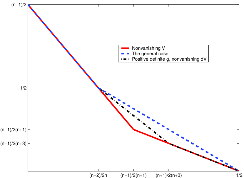
Figure 1. The $x$-axis gives $1/p$ and the $y$-axis the power of $h$ in (1.3), for $n\geq 3$.

Returning to the general setting of (1.3), the exponents $\mu(q)$ shown in Fig.1 as functions of $1/q$ depend on nondegeneracy and curvature properties of the characteristic set of $p$ intersected with the fibers of $T^{*}{\mathbb{R}}^{n}$ and the support of the localizing function $\chi$, over the support of $u$. In the case of (1.3) the continuous lines correspond to estimates localized near points at which

$$p(x_{0},\xi_{0})=0\,,\ \ d_{\xi}p(x_{0},\xi_{0})\neq 0\,,$$

$$\{\xi\;:\;p(x_{0},\xi)=0\}\subset T^{*}_{x_{0}}{\mathbb{R}}^{n}\ \text{ has a nonvanishing second fundamental form at $\xi_{0}$.}$$

That case includes Sogge’s estimate (1.1), or more generally, the case $V(x)\neq 0$ for Schrödinger operators – see Theorem 1 and Sect.5.

The dashed lines correspond to estimates localized near points at which

$$p(x_{0},\xi_{0})=0\,,\ \ d_{\xi}p(x_{0},\xi_{0})=0\,,\ \ \partial^{2}_{\xi}p(x_{0},\xi_{0})\ \text{ is nondegenerate.}$$

This case corresponds to the first estimate in (1.2) – see Theorem 1 and Sect.6.

The dotted line corresponds to estimates localized near points at which

$$p(x_{0},\xi_{0})=0\,,\ \ d_{\xi}p(x_{0},\xi_{0})=0\,,\ \ d_{x}p(x_{0},\xi_{0})\neq 0\,,\ \ \partial_{\xi}^{2}p(x_{0},\xi_{0})\ \text{is positive definite,}$$

see Theorem 2 and Sect.7. This case corresponds to the second estimate in (1.2) or the case $dV\neq 0$ for Schrödinger operators.

In this paper we are concerned with smooth symbols only. However, similar $L^{p}$ bounds for Laplacians of $C^{2}$ metrics were given by Smith in [16], and for $C^{2}$ potentials in [11]. The more robust $L^{\infty}$ bounds hold for merely $C^{1}$ metrics [17].

Finally, we add that estimates given in Theorems 1, 2, and Corollary 1 are rarely optimal for single eigenfuctions or quasimodes – see [20],[21] for a discussion and references. In fact, the problem (1.3) changes dramatically when $Pu={\mathcal{O}}_{L^{2}}(h)$ is replaced by $Pu=o_{L^{2}}(h)$ as the statement can no longer be localized.

We conclude this introduction with three examples.

Example 1. In some cases the scaling allows a transition to some global operators as in [11]. Suppose that a potential $W$ satisfies

$$\ |\partial^{\alpha}W(x)|\leq C_{\alpha}\langle x\rangle^{2-\alpha}\,,\ \ x\in{\mathbb{R}}^{n}\,,\ 1\leq i,j\leq n\,,$$

and

$$(-\Delta+W(x)-\lambda^{2})u={\mathcal{O}}(1)\,,$$

$$\ \forall\;k\,,\ \ \|\langle D\rangle u\|_{2}={\mathcal{O}}(\lambda^{2k})\,,\ \ \operatorname{supp}u\subset\{x\;:\;\delta\lambda<|x|<\lambda/\delta\}\,.$$

for some $\delta>0$. Then,

(1.14) $$\|u\|_{\infty}\leq C\lambda^{\frac{n-2}{2}}\,.$$

In fact, put $h=1/\lambda^{2}$, $V(x)=hW(x/h^{\frac{1}{2}})\psi(x/h^{\frac{1}{2}})-1$, where $\psi\in{\mathcal{C}}^{\infty}_{\rm{c}}({\mathbb{R}}^{n}\setminus\{0\})$ satisfies $\psi(x)u(x/h^{\frac{1}{2}})=u(x/h^{\frac{1}{2}})$. A simple rescaling argument and the theorem above give (1.14). If for instance $W(x)=|x|^{2}$ we obtain the natural upper bound for the spectral projections:

$${\mathchoice{1\mskip-4.0mu{\rm{l}}}{1\mskip-4.0mu{\rm{l}}}{1\mskip-4.5mu{\rm{l}}}{1\mskip-5.0mu{\rm{l}}}}_{|-\Delta+|x|^{2}-\lambda^{2}|\leq 1}={\mathcal{O}}(\lambda^{\frac{n-2}{2}})\;:\;L^{2}({\mathbb{R}}^{n})\ \longrightarrow\ L^{\infty}({\mathbb{R}}^{n})\,,\ n\geq 3\,,$$

and

$${\mathchoice{1\mskip-4.0mu{\rm{l}}}{1\mskip-4.0mu{\rm{l}}}{1\mskip-4.5mu{\rm{l}}}{1\mskip-5.0mu{\rm{l}}}}_{|-\Delta+|x|^{2}-\lambda^{2}|\leq 1}={\mathcal{O}}(1)\;:\;L^{2}({\mathbb{R}}^{n})\ \longrightarrow\ L^{\frac{2n}{n-2}}({\mathbb{R}}^{n})\,,\ n\geq 3\,.$$

Example 2. The $L^{p}$ bound in (1.9) is optimal for the ground states of

$$-h^{2}\Delta+V(x)\,,\ \ V(0)=0\,,\ \ V^{\prime\prime}(0)\gg 0\,,\ \ V|_{x\neq 0}>0\,,\ \ \liminf_{x\rightarrow\infty}V(x)>0\,,$$

that is for $u(h)$ such that

$$(-h^{2}\Delta+V(x))u(h)=E(h)u(h)\,,\ \ E(h)\leq Ch\,,\ \ \|u(h)\|_{2}=1\,.$$

see [3, Chapter 4] and references given there.

Example 3. Let us consider modes of a damped wave equation on a compact Riemannian manifold, $(M^{n},g)$,

$$(\partial_{t}^{2}+a(x)\partial_{t}-\Delta_{g})u(t,x)=0\,,\ \ u(t,x)=e^{-i\tau t}v_{\tau}(x)\,,\ \ \mathop{\rm Im}\nolimits\tau\leq 0\,,$$

$a\in{\mathcal{C}}^{\infty}(M;[0,\infty))$, see for instance [4, Sect.5.3]. Suppose that $\|v_{\tau}\|_{L^{2}}=1$, Then (1.11) shows that

$$\|v_{\tau}\|_{p}\leq C|\tau|^{\frac{1}{p}}\,,\ p=\frac{2(n+1)}{n-1}\,,\ \ \|v_{\tau}\|_{\infty}\leq C|\tau|^{(n-1)/2}\,.$$

Acknowledgments. We would like to thank Nicolas Burq, Hart F. Smith III, Christopher D. Sogge, and Steve Zelditch for helpful discussions related to the topic of this paper. The work of the first author was supported in part by the Miller Institute at the University of California, Berkeley, and that of the last two authors by the National Science Foundation grant DMS-0354539.

2. Review of semiclassical analysis

In this section we review basic aspects of semiclassical pseudodifferential calculus, referring to [3] and [4] for details.

We denote by $T^{*}{\mathbb{R}}^{k}\simeq{\mathbb{R}}^{k}\times{\mathbb{R}}^{k}$ the cotangent bundle of ${\mathbb{R}}^{k}$. The classical observables are functions of position and momentum $(x,\xi)\in T^{*}{\mathbb{R}}^{k}$. Also, denote by ${\mathcal{S}}$ and ${\mathcal{S}}^{\prime}$ the space of Schwartz functions and its dual respectively, and suppose that $a\in{\mathcal{S}}(T^{*}{\mathbb{R}}^{k})$ and . Then the left semiclassical quantization of $a$ is the operator $a(x,hD):{\mathcal{S}}^{\prime}({\mathbb{R}}^{k})\longrightarrow{\mathcal{S}}({\mathbb{R}}^{k})$ densely defined by

$$a(x,hD)u(x)\stackrel{{\scriptstyle\rm{def}}}{{=}}\frac{1}{(2\pi h)^{k}}\int e^{\frac{i}{h}\langle x-y,\xi\rangle}a(x,\xi)u(y)dyd\xi\,,\ \ u\in{\mathcal{S}}({\mathbb{R}}^{k})\,.$$

In a few places it will be convenient to use the Weyl quantization,

$$a^{w}(x,hD)u(x)\stackrel{{\scriptstyle\rm{def}}}{{=}}\frac{1}{(2\pi h)^{k}}\int e^{\frac{i}{h}\langle x-y,\xi\rangle}a\left(\frac{x+y}{2},\xi\right)u(y)dyd\xi\,,\ \ u\in{\mathcal{S}}({\mathbb{R}}^{k})\,.$$

One of its advantages is the selfadjointness of $a^{w}(x,hD)$ for real values $a$’s.

This definition can be extended to a large class of observables. A function, $m:T^{*}{\mathbb{R}}^{k}\longrightarrow[0,\infty)$ is called an order function if for all $(x,\xi)\,,\ (y,\eta)\in T^{*}{\mathbb{R}}^{k}$,

$$m(x,\xi)\leq C(1+|x-y|+|\xi-\eta|)^{N}m(y,\eta)\,,$$

for some fixed $C$ and $N$. We say that $a\in{\mathcal{C}}^{\infty}({\mathbb{R}}^{k})$ is a symbol in class $S(m)$ if

$$|\partial^{\alpha}_{x,\xi}a(x,\xi)|\leq C_{\alpha}m(x,\xi)\,,\ \ \alpha\in{\mathbb{N}}^{2k}\,.$$

Unless specifically stated, we always allow the symbols to depend on $h$. The continuous map

$${\mathcal{S}}(T^{*}{\mathbb{R}}^{k})\ni a\longmapsto a(x,hD)\in{\mathcal{L}}({\mathcal{S}}({\mathbb{R}}^{k}),{\mathcal{S}}({\mathbb{R}}^{k}))\,,$$

extends to a continuous map

$$S(m)\ni a\longmapsto a(x,hD)\in{\mathcal{L}}({\mathcal{S}}({\mathbb{R}}^{k}),{\mathcal{S}}({\mathbb{R}}^{k}))\ \,,$$

which satisfies the following fundamental composition property: if $m_{j}$, $j=1,2$ are two order functions, and $a_{j}\in S(m_{j})$, $j=1,2$, then

(2.1) $$a_{1}(x,hD)a_{2}(x,hD)=b(x,hD)\,,\ \ b\in S(m_{1}m_{2})\,.$$

Moreover we have an asymptotic formula for $b(x,\xi)$ given by

(2.2) $$b(x,\xi)\sim\sum_{\alpha\in{\mathbb{N}}^{k}}\frac{1}{\alpha!}\partial_{\xi}^{\alpha}a_{1}(x,\xi)(hD_{x})^{\alpha}a_{2}(x,\xi)\,.$$

We also have the mapping property:

(2.3) $$a\in S(1)\;\Longrightarrow\;a(x,hD)={\mathcal{O}}(1)\;:\;L^{2}({\mathbb{R}}^{k})\longrightarrow L^{2}({\mathbb{R}}^{k})\,.$$

Suppose that $a\in S(1)$ and that $|a(x,\xi)|\geq 1/C$ for all $(x,\xi)\in T^{*}{\mathbb{R}}^{k}$. Then

$$a(x,hD)^{-1}\;:\;L^{2}({\mathbb{R}}^{k})\;\longrightarrow\;L^{2}({\mathbb{R}}^{k})\,,$$

exists if $h$ is small enough. In fact, by our hypothesis $c(x,\xi)\stackrel{{\scriptstyle\rm{def}}}{{=}}1/a(x,\xi)\in S(1)$, and by (2.1) and (2.2),

$$a(x,hD)c(x,hD)=I+hr(x,hD)\,,\ \ r\in S(1)\,.$$

By (2.3), $r(x,hD)={\mathcal{O}}(1):L^{2}\rightarrow L^{2}$, and hence $I+hr(x,hD)$ is invertible for $h$ small enough. This gives $a(x,hD)^{-1}=c(x,hD)(I+hr(x,hD))^{-1}$. The use of semiclassical Beals’s Lemma [3, Proposition 8.3], [4, Theorem 8.9], shows more: $a(x,hD)^{-1}=b(x,hD)$, $b\in S(1)$.

In this note we will also need a microlocal version of this result:

Lemma 2.1.

Suppose that $\chi\in S(1)$, $m$ is an order function, and that $a\in S(m)$ satisfies $|a(x,\xi)|\geq m(x,\xi)/C$ for $(x,\xi)\in\operatorname{supp}\chi$. Then there exists $b\in S(1/m)$ such that

(2.4) $$\begin{split}&b(x,hD)a(x,hD)\chi(x,hD)=\chi(x,hD)+{\mathcal{O}}_{L^{2}\rightarrow L^{2}}(h^{\infty})\,,\\ &a(x,hD)b(x,hD)\chi(x,hD)=\chi(x,hD)+{\mathcal{O}}_{L^{2}\rightarrow L^{2}}(h^{\infty})\,.\end{split}$$

When $\chi\in{\mathcal{C}}^{\infty}_{\rm{c}}(T^{*}{\mathbb{R}}^{n})$ we can replace ${\mathcal{O}}_{L^{2}\rightarrow L^{2}}(h^{\infty})$ by ${\mathcal{O}}_{{\mathcal{S}}^{\prime}\rightarrow{\mathcal{S}}}(h^{\infty})$.

Proof.

We give the proof in the case of $\chi\in{\mathcal{C}}^{\infty}_{\rm{c}}$ and we first note that $a\chi\in S((1+|x|+|\xi|)^{-M})$ for any $M$. We then inductively construct $b_{j}\in S(1)$ such that

$$\left(\sum_{j=0}^{N}h^{j}b_{j}(x,hD)\right)a(x,hD)\chi(x,hD)=\chi(x,hD)+h^{N}r_{N}(x,hD)\,,$$

$r_{N}\in S((1+|x|+|\xi|)^{-M})$, for any $M$. The symbol $b\in S(1)$ satisfying

$$b(x,\xi)\sim\sum_{j=0}^{\infty}b_{j}(x,\xi)$$

gives (2.4). ∎

The next lemma provides basic semiclassical $L^{p}$ estimates:

Lemma 2.2.

Suppose that $a\in{\mathcal{S}}(T^{*}{\mathbb{R}}^{k})$. Then for $1\leq q\leq p\leq\infty$,

(2.5) $$a(x,hD)={\mathcal{O}}(h^{k\left(1/p-1/q\right)})\;:\;L^{q}({\mathbb{R}}^{k})\;\longrightarrow\;L^{p}({\mathbb{R}}^{k})\,.$$

Proof.

We first recall that

$$a(x,hD)u(x)=h^{-k}\int K(x,(x-y)/h)u(y)dy\,,$$

where

$$K(x,z)\stackrel{{\scriptstyle\rm{def}}}{{=}}\frac{1}{(2\pi)^{k}}\int a(x,\xi)e^{i\langle\xi,z\rangle}d\xi\,.$$

In particular $K\in{\mathcal{S}}({\mathbb{R}}^{k}\times{\mathbb{R}}^{k})$, and $|K(x,z)|\leq C_{N}(1+|z|)^{-N}$ for any $N$ with $C_{N}$ independent of $x$. This means that

$$\|a(x,hD)u\|_{L^{p}}\leq C_{N}h^{-k}\|(1+|\bullet/h|)^{-N}*u\|_{p}\,.$$

The Young inequality,

(2.6) $$\|f*u\|_{L^{p}}\leq\|f\|_{r}\|u\|_{q}\,,\ \ 1\leq p,q,r\leq\infty\,,\ \ \frac{1}{p}+1=\frac{1}{r}+\frac{1}{q}\,,$$

and the calculation

$$h^{-k}\|(1+|\bullet/h|)^{-N}\|_{L^{r}}=Ch^{-k}h^{k/r}=Ch^{k(1/p-1/q)}\,,$$

give (2.5). ∎

A microlocal version of the localization assumption (1.6) is given as follows

(2.7) $$\exists\;\chi\in{\mathcal{C}}^{\infty}_{\rm{c}}(T^{*}{\mathbb{R}}^{k})\,,\ N\geq 0\,,\ \ u(h)=\chi(x,hD)u(h)+{\mathcal{O}}_{\mathcal{S}}(h^{\infty})\,,\ \ \|u(h)\|_{2}={\mathcal{O}}(h^{-N})\,.$$

The bound in $L^{2}$ is needed as otherwise the statement ${\mathcal{O}}_{\mathcal{S}}(h^{\infty})$ has no meaning, in view of scaling. We also need it to guarantee that the residual terms in the semiclassical calculus give ${\mathcal{O}}(h^{\infty})$ bounds when applied to $u(h)$. Except in Theorem 3 we can simply assume that $\|u(h)\|_{L^{2}}=1$.

This assumption combined with Lemma 2.2 has the following consequence which is a semiclassical version of Sobolev embedding. In fact, it is equivalent to Sobolev embedding for functions localized in frequency to a dyadic corona.

Lemma 2.3.

Suppose that a family $u=u(h)$ satisfies (2.7). Then for any $1\leq q\leq p\leq\infty$,

(2.8) $$\|u\|_{L^{p}}\leq Ch^{k(1/p-1/q)}\|u\|_{L^{q}}+{\mathcal{O}}(h^{\infty})\,.$$

Proof.

The estimates for $\|\chi(x,hD_{x})u\|_{p}$ follows from Lemma 2.2 and

$$\|(1-\chi)(x,hD)u\|_{q}=O(h^{\infty})\,,$$

from (2.7) ∎

As an application of Lemmas 2.1 and 2.3 we state the following elliptic semiclassical $L^{p}$ estimate. It shows that to obtain general estimates in the remaining sections we can assume that $u$ is localized to a neighbourhood of a characteristic point of $P$.

Theorem 3.

Suppose that $u$ satisfies the localization condition (2.7) and that

$$Pu={\mathcal{O}}_{L^{2}}(h)\,,\ \ |p(x,\xi)|\geq 1/C\,,\ \ (x,\xi)\in\operatorname{supp}\chi\,.$$

Then

$$\|u\|_{p}={\mathcal{O}}(h^{1-n(1/2-1/p)})\,.$$

The next lemma is a global semiclassical version of a Sobolev embedding estimate (see for instance [6, Theorem 4.5.13]):

Lemma 2.4.

Suppose that $\Omega_{1}$ and $\Omega_{2}$ have properties stated in Lemma 2.6. Then for $u\in{\mathcal{C}}^{\infty}({\mathbb{R}}^{n})$

$$\|u\|_{L^{p}(\Omega_{1})}\leq C_{1}h^{-n(1/2-1/p)}\sum_{|\alpha|\leq m}\|(hD)^{\alpha}u\|_{L^{2}(\Omega_{2})}\,,\ \ \frac{1}{2}-\frac{m}{n}\leq\frac{1}{p}\leq\frac{1}{2}\,,\ \ p<\infty\,.$$

When $u\in{\mathcal{C}}^{\infty}_{\rm{c}}({\mathbb{R}}^{n})$, and $1/2-m/n=1/p$, $p<\infty$, we can replace $|\alpha|\leq m$ in the sum by $|\alpha|=m$.

Proof.

We can assume that $u\in{\mathcal{C}}^{\infty}_{\rm{c}}(\Omega_{2})$ and then can consider $\Omega_{1}=\Omega_{2}={\mathbb{R}}^{n}$. In that case the estimate with $h=1$ is a standard Sobolev inequality. Applying it to $v_{h}(x)=u(hx)$ gives the lemma: $(hD_{x})^{\alpha}u=D_{x}^{\alpha}v_{h}$,

$$\|v_{h}\|_{H^{m}({\mathbb{R}}^{n})}=h^{-\frac{n}{2}}\sum_{|\alpha|\leq m}\|(hD_{\alpha})u\|_{L^{2}({\mathbb{R}}^{n})}\,,\ \ \|v_{h}\|_{L^{p}({\mathbb{R}}^{n})}=h^{-\frac{n}{p}}\|u\|_{L^{p}({\mathbb{R}}^{n})}\,.$$

∎

For future reference we state also another basic fact. Let

$${\mathcal{F}}_{h}v(\xi)\stackrel{{\scriptstyle\rm{def}}}{{=}}\frac{1}{(2\pi h)^{n/2}}\int_{{\mathbb{R}}^{n}}v(x)e^{\frac{i}{h}\langle x,\xi\rangle}dx\,,$$

be the semiclassical Fourier transform, normalized to be unitary on $L^{2}({\mathbb{R}}^{n})$. The semiclassical Sobolev spaces are defined using the following norm

$$\|u\|_{H^{s}_{h}({\mathbb{R}}^{n})}^{2}\stackrel{{\scriptstyle\rm{def}}}{{=}}\int_{{\mathbb{R}}^{n}}(1+|\xi|^{2})^{s}|{\mathcal{F}}_{h}v(\xi)|^{2}d\xi\,.$$

If $s$ is a nonegative integer then clearly

$$\|u\|_{H^{s}_{h}({\mathbb{R}}^{n})}\simeq\sum_{|\alpha|\leq s}\|(hD)^{\alpha}u\|_{2}\,.$$

Lemma 2.5.

For $s>n/2$ we have

$$\|u\|_{\infty}\leq Ch^{-n/2}\|u\|_{H^{s}_{h}({\mathbb{R}}^{n})}\,.$$

Proof.

We follow the usual procedure keeping track of the parameter $h$:

$$\begin{split}\|u\|_{\infty}^{2}&\leq\frac{1}{(2\pi h)^{n}}\left(\int_{{\mathbb{R}}^{n}}|{\mathcal{F}}_{h}u(\xi)|d\xi\right)^{2}\\ &\leq\frac{1}{(2\pi h)^{n}}\int_{{\mathbb{R}}^{n}}(1+|\xi|^{2})^{-s}d\xi\int_{{\mathbb{R}}^{n}}(1+|\xi|^{2}))^{s}|{\mathcal{F}}_{h}u(\xi)|^{2}d\xi=\frac{C}{h^{n}}\|u\|_{H^{s}_{h}({\mathbb{R}}^{n})}^{2}\,.\end{split}$$

∎

Finally, we state without proof a semiclassical version of standard elliptic estimates (see for instance [7, Theorem 17.1.3]):

Lemma 2.6.

Suppose that a differential operator, $P(h)=\sum_{|\alpha|\leq m}a_{\alpha}(x,h)(hD_{x})^{\alpha}$, satisfies,

(2.9) $$\forall\,|\alpha|\leq m\,,\ \beta\in{\mathbb{N}}^{n}\,,\ \ \partial_{x}^{\beta}a_{\alpha}(x,h)={\mathcal{O}}(1)\,,\ \ |\sum_{|\alpha|=m}a_{\alpha}(x,h)\xi^{\alpha}|\geq|\xi|^{m}/C\,,\ \ C>0\,,$$

uniformly for $x\in K$, for any $K\Subset{\mathbb{R}}^{n}$. Then for any bounded open sets $\Omega_{1}$, $\Omega_{2}$, $\overline{\Omega}_{1}\Subset\Omega_{2}$, and $u\in{\mathcal{C}}^{\infty}({\mathbb{R}}^{n})$, we have

$$\sum_{|\alpha|\leq m}\|(hD)^{\alpha}u\|_{L^{2}(\Omega_{1})}\leq C_{0}\left(\|P(h)u\|_{L^{2}(\Omega_{2})}+\|u\|_{L^{2}(\Omega_{2})}\right)\,,$$

where $C_{0}$ depends only on constants in (2.9) for $K=\overline{\Omega}_{2}$, $\Omega_{2}$, and $\Omega_{1}$.

3. $L^{\infty}$ estimates in the principal type case

In this section we prove $L^{\infty}$ bounds under a principal type assumption. We remark that this assumption is always satisfied in the case of the Laplacian on a Riemannian manifold for which $p(x,\xi)=\sum g^{ij}(x)\xi_{i}\xi_{j}-1$. The simple direct proof implies, rather than uses, the optimal upper bound on the number of eigenvalues of an elliptic operator in an interval of size $h$ – see Corollary 2 at the end of this section.

Theorem 4.

Let $m=m(x,\xi)$ an order function, and let $u(h)\in L^{2}({\mathbb{R}}^{n})$ satisfy the frequency localization condition (2.7). Suppose that $p\in S(m)$ is real valued, and that

(3.1) $$p(x,\xi)=0\,,\ \ (x,\xi)\in\operatorname{supp}\chi\ \Longrightarrow\partial_{\xi}p(x,\xi)\neq 0\,.$$

Then

(3.2) $$\|u(h)\|_{L^{\infty}}\leq Ch^{-(n-1)/2}\left(\|u(h)\|_{L^{2}}+\frac{1}{h}\|p(x,hD)u(h)\|_{L^{2}}\right)\,.$$

Remark. The bound given in Theorem 4 is already optimal in the simplest case in which the assumptions are satisfied: $p(x,\xi)=\xi_{1}$. Indeed, write $x=(x_{1},x^{\prime})$ and let $\chi_{1}\in{\mathcal{C}}^{\infty}_{\rm{c}}({\mathbb{R}})$, and $\chi\in{\mathcal{C}}^{\infty}_{\rm{c}}({\mathbb{R}}^{n-1})$. Then

$$u(h):=h^{-(n-1)/2}\chi_{1}(x_{1})\chi(x^{\prime}/h)$$

satisfies

$$p(x,hD)u(h)=hD_{x_{1}}u(h)=O_{L^{2}}(h)\,,\ \ \|u(h)\|_{2}=O(1)\,,$$

and for any non-trivial choices of $\chi_{1}$ and $\chi$,

$$\|u(h)\|_{\infty}\simeq h^{-(n-1)/2}\,.$$

The condition (3.1) is in general necessary as shown by another simple example. Let $p(x,\xi)=x_{1}$, and

$$u(h)=h^{-n/2}\chi_{1}(x_{1}/h)\chi(x^{\prime}/h)\,.$$

Then

$$P(h)u(h)=hh^{-n/2}(t\chi_{1}(t))|_{t=x_{1}/h}\chi(x^{\prime}/h)=O_{L^{2}}(h)\,,\ \ \|u(h)\|_{2}=O(1)\,,$$

and

$$\|u(h)\|_{\infty}\simeq h^{-n/2}\,,$$

which is the general bound of Lemma 2.3.

Proof of Theorem 4: First we observe that we can assume that $u(h)$ is compactly supported. We also note that the estimate hypothesis on $u(h)$ is local in phase space: if $\chi\in{\mathcal{C}}^{\infty}_{\rm{c}}(T^{*}{\mathbb{R}}^{k})$ then, normalizing to $\|u(h)\|_{2}=1$,

$$\begin{split}p(x,hD)\chi^{w}(x,hD)u(h)&=\chi^{w}(x,hD)p(x,hD)u(h)+[p(x,hD),\chi^{w}(x,hD)]u(h)\\ &={\mathcal{O}}(1)(h\|u\|_{2}+\|p(x,hD)u\|_{2})\,,\end{split}$$

Hence it is enough to prove the theorem for $u(h)$ replaced by $\chi^{w}u(h)$, where $\chi$ is supported near a given point in $K$ as a partition of unity argument will then give the bound on $u(h)$. A partition of unity, in this case, means a set of functions,

$$\{\chi_{j}\}_{j=0}^{N}\subset{\mathcal{C}}^{\infty}_{\rm{c}}(T^{*}{\mathbb{R}}^{n})\,,$$

such that

(3.4) $$\begin{gathered}\sum_{j=1}^{N}\chi_{j}(x,\xi)=\chi_{0}(x,\xi)\,,\ \ \operatorname{supp}\chi_{j}\subset U_{j}\,,\ \ \operatorname{supp}\chi_{0}\subset U_{0}\stackrel{{\scriptstyle\rm{def}}}{{=}}\bigcup_{j=1}^{N}U_{j}\,,\end{gathered}$$

where $U_{0}$ is a neighbourhood of $\operatorname{supp}\chi$, a compact set, in which (3.1) holds.

Suppose that $p\neq 0$ on the support of $\chi$. We can quote Theorem 3 but for the reader’s convenience present an argument. From the ellipticity and Lemma 2.1 we see that $p(x,hD)\chi^{w}u(h)={\mathcal{O}}_{L^{2}}(h)$ implies that $\chi^{w}u(h)={\mathcal{O}}_{L^{2}}(h)$. Lemma 2.3 then shows that

$$\|\chi^{w}u(h)\|_{\infty}\leq Chh^{-n/2}\leq Ch^{-(n-1)/2}\,.$$

Now suppose that $p$ vanishes in the support of $\chi$. By applying a linear change of variables we can assume that $p_{\xi_{1}}\neq 0$ there. The implicit function theorem shows that

(3.5) $$p(x,\xi)=e(x,\xi)(\xi_{1}-a(x,\xi^{\prime}))\,,\ \ \xi=(\xi_{1},\xi^{\prime})\,,\ \ e(x,\xi)>0\,,$$

holds in a neighbourhood of $\operatorname{supp}\chi$. We extend $e$ arbitrarily to $e\in S$, $e\geq 1/C$, and $a(x,\xi^{\prime})$ to a real valued $a(x,\xi^{\prime})\in S$. The pseudodifferential calculus shows that

$$\begin{split}e^{w}(x,hD)(hD_{x_{1}}-a(x,hD_{x^{\prime}}))(\chi^{w}u(h))&=p(x,hD)(\chi^{w}u(h))+{O}_{L^{2}}(h)\\ &={O}_{L^{2}}(h)\,,\end{split}$$

and since $e^{w}$ is elliptic,

(3.6) $$(hD_{x_{1}}-a(x,hD_{x^{\prime}}))(\chi^{w}u(h))=O_{L^{2}}(h)\,.$$

The proof will be completed if we show that

(3.7) $$\|(\chi^{w}u)(x_{1},\bullet)\|_{L^{2}({\mathbb{R}}^{n-1})}=O(1)\,,$$

and for that we need another elementary

Lemma 3.1.

Suppose that $a\in S({\mathbb{R}}\times T^{*}{\mathbb{R}}^{k})$ is real valued, and that

$$(hD_{t}+a^{w}(t,x,hD_{x}))u(t,x)=f(t,x)\,,\ \ u(0,x)=u_{0}(x)\,,$$

$$f\in L^{2}({\mathbb{R}}\times{\mathbb{R}}^{k})\,,\ \ u_{0}\in L^{2}({\mathbb{R}}^{k})\,.$$

Then

(3.8) $$\|u(t,\bullet)\|_{L^{2}({\mathbb{R}}^{k})}\leq\frac{\sqrt{t}}{h}\|f\|_{L^{2}({\mathbb{R}}\times{\mathbb{R}}^{k})}+\|u_{0}\|_{L^{2}({\mathbb{R}}^{k})}\,.$$

Proof.

Since $a^{w}(t,x,hD)$ is family of bounded operators on $L^{2}({\mathbb{R}}^{k})$ existence of solutions follows from existence theory for (linear) ordinary differential equations in $t$. Suppose first that $f\equiv 0$. Then

$$\begin{split}\frac{1}{2}\frac{d}{dt}\|u(t)\|_{L^{2}({\mathbb{R}}^{k})}^{2}&=\mathop{\rm Re}\nolimits\langle\partial_{t}u(t),u(t)\rangle_{L^{2}({\mathbb{R}}^{k})}\\ &=\frac{1}{h}\mathop{\rm Re}\nolimits\langle ia^{w}(x,hD)u(t),u(t)\rangle=0\,.\end{split}$$

Thus, if we put $E(t)u_{0}:=u(t)$,

$$\|E(t)u_{0}\|_{L^{2}({\mathbb{R}}^{k})}=\|u_{0}\|_{L^{2}({\mathbb{R}}^{k})}\,.$$

If $f\neq 0$, Duhamel’s formula gives

$$u(t)=E(t)u_{0}+\frac{i}{h}\int_{0}^{t}E(t-s)f(s)ds\,,$$

and hence

$$\|u(t)\|_{L^{2}({\mathbb{R}}^{k})}\leq\|u_{0}\|_{L^{2}({\mathbb{R}}^{k})}+\int_{0}^{t}\|f(s)\|_{L^{2}({\mathbb{R}}^{k})}\,.$$

The estimate (3.8) is an immediate consequence. ∎

The estimate (3.7) is immediate from the lemma and (3.6). We now apply Lemma 2.3 in $x^{\prime}$ variables only, that is with $k=n-1$. That is allowed since we clearly have

$$\|(1-\psi(hD^{\prime}))\chi^{w}u(h)(x_{1},\bullet)\|_{L^{2}({\mathbb{R}}^{n-1})}=O(h^{\infty})\,,$$

uniformly in $x_{1}$.      

As an application we give a proof of a well known result about the density of eigenvalues near a nondegenerate energy level – see [8, Chapter 4] for a full discussion. For simplicity we assume that our operator is defined on a compact manifold $X$ – see [4, Appendix D] for an introduction to semiclassical analysis on manifolds. The symbol classes are now defined as

$$S^{m,k}(T^{*}X)=\{a\in{\mathcal{C}}^{\infty}(T^{*}X)\;:\;|\partial_{x}^{\alpha}\partial_{\xi}^{\beta}a|\leq h^{-k}C_{\alpha\beta}(1+|\xi|)^{m-|\beta|}\}\,,$$

with corresponding operators denoted by $\Psi^{m,k}(X,\Omega_{\frac{1}{2}}X)$, where to avoid a choice of a density we act on half densities on $X$ (see [4, Sect.8.1]). The principal symbol of $P\in\Psi^{m,k}(X,\Omega_{\frac{1}{2}})$ is then defined in $S^{m,k}/S^{m-1,k-1}(T^{*}X)$. The example to keep in mind is of course

$$P=-h^{2}\Delta-1\in\Psi^{2,0}(X)\,.$$

Corollary 2.

Let $P\in\Psi^{m,0}(X,\Omega_{\frac{1}{2}}X)$ be a semiclassical selfadjoint pseudodifferential operator on a compact $n$ dimensional manifold $X$ with a real principal symbol $p\in S^{m,0}(T^{*}X)$ (well defined modulo $S^{m-1,-1}(T^{*}X)$) satisfying

$$|p(x,\xi)|\geq(1+|\xi|)^{m}/C-C\,,\ \ (x,\xi)\in T^{*}X\,.$$

Let $\operatorname{Spec}(P)\subset{\mathbb{R}}$ be the spectrum of $P$ which is a discrete set. If

$$p(x,\xi)=E\in{\mathbb{R}}\implies d_{\xi}p(x,\xi)\neq 0\,,$$

then

$$|[E-h,E+h]\cap\operatorname{Spec}(P)|={\mathcal{O}}(h^{1-n})\,.$$

Proof.

We reverse the standard argument for obtaining $L^{\infty}$ bounds from remainder estimates for the spectral projection – see [18]. Under the assumptions on $P$, the resolvent $(P-z)^{-1}$ is compact for $z\notin{\mathbb{R}}$ (for instance using Lemma 2.1 with $m(x,\xi)=\langle\xi\rangle^{m}$). Hence the spectrum consists of isolated eigenvalues, $\lambda$, with smooth eigenfuctions half densities, $\phi_{\lambda}$. We define the spectral projection,

$$\Pi_{h}(x,y)=\sum_{|\lambda-E|\leq h}\phi_{\lambda}(x)\overline{\phi_{\lambda}(y)}\,.$$

Theorem 4 shows that

$$\Pi_{h}={\mathcal{O}}(h^{-(n-1)/2})\;:\;L^{2}(X,\Omega_{\frac{1}{2}}X)\rightarrow L^{\infty}(X)\,.$$

Here we chose a trivialization of the half-density bundle which identified half densities with functions, allowing a map into $L^{\infty}$. Hence,

$$\Pi_{h}(x,x)=\int_{X_{y}}\Pi_{h}(x,y)\Pi_{h}(y,x)=F_{h}(x)|dx|\,,\ \ |F_{h}(x)|\leq\|\Pi_{h}\|_{L^{2}\rightarrow L^{\infty}}^{2}\leq Ch^{-n+1}\,,$$

and

$$\begin{split}|[E-h,E+h]\cap\operatorname{Spec}(P)|&=\int_{X}\Pi_{h}(x,x)=\int_{X}F_{h}(x)|dx|\\ &\leq\operatorname{vol}(X)\|F_{h}\|_{\infty}={\mathcal{O}}(h^{-n+1})\,.\end{split}$$

Here the volume was computed using the same trivialization of the density bundle. ∎

The same proof can be applied in other situations in which we have precise $L^{\infty}$ bounds, for instance under the assumptions of Theorems 1, 6, $n>2$. That however does not add anything new to the results of Ivrii [8]. Brummelhuis-Paul-Uribe [1] obtained precise asymptotics when the critical set of $p$ has a nice structure and that paper can be used to construct operators for which $\log(1/h)$ appears in $L^{\infty}$ bounds. However, both references suggest that the $\log(1/h)$ term in Theorem 1 when $n=2$ does not occur for Schrödinger operators.

Finally we remark that in the case of nonselfadjoint operators $L^{\infty}$ estimates do not seem to give bounds on the number of eigenvalues in small regions – see [15] for a discussion of such estimates and references in the context of resonances.

4. Semiclassical Strichartz estimates

To prove Theorems 1 and 2, or rather their more general versions in Sections 5, 6, and 7, we use Strichartz estimates. Unlike the $L^{\infty}$ bound of the previous section which involved an energy estimate only they rely on the nondegeneracy of $\partial_{\xi}^{2}p$.

Semiclassical Strichartz estimates for the Schrödinger propagator of $P=-h^{2}\Delta_{g}-1$ appeared explicitely in the work of Burq, Gérard, and Tzvetkov [2] who used them to prove existence results for non-linear Schrödinger equations on two and three dimensional compact manifolds. A more robust phase space representation of Schrödinger propagators applicable to a wider range of operators is given in [10] and [22]. We refer to these papers for pointers to the vast literature on Strichartz estimates and their applications.

Here we give a consequence of the well known parametrix construction recalled in Proposition 4.2 and of the abstract Strichartz estimates of [9]. For the reader’s convenience we first recall the abstract Strichartz estimate, slightly modified for the semiclassical application:

Proposition 4.1.

Let $(X,{\mathcal{M}},dm)$ be a $\sigma$-finite measure space, and let

$$U\in L^{\infty}({\mathbb{R}},{\mathcal{B}}(L^{2}(X,dm))$$

satisfy

(4.3) $$\begin{gathered}\|U(t)\|_{{\mathcal{B}}(L^{2}(X))}\leq A\,,\ \ t\in{\mathbb{R}}\,,\\ \|U(t)U(s)^{*}f\|_{L^{\infty}(X,\mu)}\leq Ah^{-\mu}(|t-s|+h)^{-\sigma}\|f\|_{L^{1}(X,dm)}\,,\ \ t,s\in{\mathbb{R}}\,,\end{gathered}$$

where $A,\sigma>0$, $\mu\geq 0$ are fixed.

The for every pair $p,q$ satisfying

$$\frac{2}{p}+\frac{2\sigma}{q}=\sigma\,,\ \ 2\leq p\leq\infty\,,\ \ 1\leq q\leq\infty\,,\ \ (p,q)\neq(2,\infty)\,,$$

we have

(4.4) $$\left(\int_{{\mathbb{R}}}\|U(t)f\|_{L^{q}(X,dm)}^{p}dt\right)^{\frac{1}{p}}\leq Bh^{-\frac{\mu}{p\sigma}}\|f\|_{L^{2}(X,dm)}\,.$$

When $(p,q)=(2,\infty)$, and $\mu=2$, we have the same estimates with the $h$ dependent constant replaced by $(\log(1/h)/h)^{1/2}$.

To explain the logarithmic correction term for $(p,q)=(2,\infty)$, that is $\sigma=1$, we recall the proof in in that case referring the reader to [9] for a complete argument. We also remark that in (4.3) $(|t-s|+h)^{-\sigma}$ can be replaced by $|t-s|^{-\sigma}$ except for the case of $(2,\infty)$.

Proof of the case $\sigma=1$, $p=2$: The estimate we want reads

$$\|U(t)f\|_{L^{2}({\mathbb{R}}_{t},L^{\infty}(X))}\leq B\|f\|_{L^{2}(X)}\,.$$

This is equivalent to

$$\int_{{\mathbb{R}}\times X}U(t)f(x)\;G(t,x)\;dm(x)dt\leq\|f\|_{L^{2}(X)}\|G\|_{L^{2}({\mathbb{R}},L^{1}(X))}\,,$$

for all $G\in L^{2}({\mathbb{R}},L^{\infty}(X))$, and that in turn means that

$$\|\int_{\mathbb{R}}U(t)^{*}G(t)dt\|_{L^{2}(X)}\leq C\|G\|_{L^{2}({\mathbb{R}},L^{1}(X))}\,,$$

or in other words that

(4.5) $$T:L^{2}({\mathbb{R}},L^{\infty}(X))\longrightarrow L^{2}(X)\,,\ \ TG(x):=\int_{\mathbb{R}}U(t)^{*}G(t,x)dt\,.$$

We note that $T^{*}f(s,x):=U(s)f(x)$, and that the mapping property (4.5) is equivalent to

$$\langle T^{*}TG,F\rangle_{L^{2}({\mathbb{R}}\times X)}\leq C\|G\|_{L^{2}({\mathbb{R}},L^{1}(X))}\|F\|_{L^{2}({\mathbb{R}},L^{1}(X))}\,,$$

which is the same as

(4.6) $$\begin{split}&\left|\int_{\mathbb{R}}\!\int_{\mathbb{R}}\langle U(t)^{*}G(t),U(s)^{*}F(s)\rangle\;dtds\right|\leq C\|G\|_{L^{2}({\mathbb{R}},L^{1}(X))}\|F\|_{L^{2}({\mathbb{R}},L^{1}(X))}\,.\end{split}$$

The hypothesis (with $\sigma=1$) can be restated as

$$\begin{split}&|\langle U(t)^{*}G(t),U(s)^{*}F(s)\rangle|\leq Ch^{-1}(h+|t-s|)^{-1}\|G(t)\|_{L^{1}(X)}\|F(s)\|_{L^{1}(X)}\,.\end{split}$$

Now now apply the Young inequality in $t$ (see (2.6) above) with $p=q=2$ and $r=1$, noting that $\|\psi(t)(h+|\bullet|)^{-1}\|_{L^{1}({\mathbb{R}})}\leq C\log(1/h)$. That gives (4.6) completing the proof.

     

We also need the semiclassical parametrix construction which is classical [sic!] and where we follow [5, Appendix a] – see also [14, Proposition 7.3], and for a textbook presentation [4, Sect.10.2]. As emphasized in [10] for the dispersive estimates of the type used here, we only need very basic information about the amplitude, far from the precise results needed, for instance, in the study of trace formulæ [14].

Proposition 4.2.

Suppose that $F(t,r)$ is defined by

$$hD_{t}F(t,r)+P(t)F(t,r)=0\,,\ \ F(r,r)=G(r)(x,hD)\,,\ G(r)\in{\mathcal{C}}^{\infty}_{\rm{c}}(T^{*}{\mathbb{R}}^{k})\,.$$

Let us also assume that $p_{t}=\sigma(P(t))$, the Weyl symbol (with a possible dependence on $h$ in the subprincipal symbol part) of $P(t)$, is real. Then there exists $t_{0}>0$, independent of $h$, such that for $0\leq t\leq t_{0}$,

(4.7) $$F(t,r)u(x)={\frac{1}{(2\pi h)^{k}}}\iint e^{{\frac{i}{h}}(\phi(t,r,x,\eta)-y\cdot\eta)}b(t,x,\eta;h)u(y)dyd\eta+E(t,r)u(x)\,,$$

where

(4.8) $$\partial_{t}\phi(t,r,x,\eta)+p_{t}(x,\partial_{x}\phi(t,r,x,\eta)=0,\ \ \ \phi(r,r,x,\eta)=x\cdot\eta\,,$$

$b\in{\mathcal{C}}^{\infty}_{\rm{c}}({\mathbb{R}}\times T^{*}{\mathbb{R}}^{n})$, and $E(t,r)={\mathcal{O}}(h^{\infty}):{\mathcal{S}}^{\prime}\rightarrow{\mathcal{S}}$.

Proof.

The equation (4.8) is the standard eikonal equation for which we find a (possibly $h$-dependent) solution $\phi$. The amplitude $b$ has to satisfy

$$(hD_{t}+p_{t}^{w}(x,hD))(e^{i\phi(t,x,\eta)/h}b(t,x,\eta;h))=0\,,$$

which is the same as

$$(\partial_{t}\phi+hD_{t}+e^{-i\phi/h}p_{t}^{w}(x,hD)e^{i\phi/h})(b)=0\,.$$

The Weyl symbol of $e^{-i\phi/h}p_{t}^{w}e^{i\phi/h}$ is

$$q_{t}(x,\xi)=p_{t}(x,\phi_{x}^{\prime}+\xi)+{\mathcal{O}}(h^{2})\,,$$

and using that $\partial_{t}\phi=-p_{t}(x,\partial_{x}\phi)$, we get

$$(hD_{t}+f_{t}^{w}(x,hD))b={\mathcal{O}}(h^{2})\,,$$

with $f_{t}(x,\xi)=p_{t}(x,\phi_{x}^{\prime}+\xi)-p_{t}(x,\phi^{\prime}_{x})$, and with $\eta$ considered as a parameter. This can be solved asymptotically in $h$. ∎

Proposition 4.3.

Suppose that $\chi\in{\mathcal{C}}^{\infty}_{\rm{c}}(T^{*}{\mathbb{R}}^{k})$, and that (6.1) holds in $\operatorname{supp}(\chi)$. With $P=p(x,hD)$, let $U(t)$ be given by Proposition 4.2. Then for $\psi\in{\mathcal{C}}^{\infty}_{\rm{c}}({\mathbb{R}})$ with support sufficiently close to $0$, and

$$U(t,r):=\psi(t)F(t,r)\chi^{w}(x,hD)\ \text{ or }\ U(t,r):=\psi(t)\chi^{w}(x,hD)F(t,r)$$

we have

(4.11) $$\begin{gathered}\sup_{r\in I}\left(\int_{{\mathbb{R}}}\|U(t,r)f\|_{L^{q}({\mathbb{R}}^{n})}^{p}dt\right)^{\frac{1}{p}}\leq Bh^{-\frac{1}{p}}\|f\|_{L^{2}({\mathbb{R}}^{n})}\,,\\ \frac{2}{p}+\frac{k}{q}=\frac{k}{2}\,,\ \ 2\leq p\leq\infty\,,\ \ 1\leq q\leq\infty\,,\ (p,q)\neq(2,\infty)\,.\end{gathered}$$

When $(p,q)=(2,\infty)$, that is for $k=2$, we have the same estimate with $h^{-1/2}$ replaced by $(\log(1/h)/h)^{1/2}$.

Proof.

In view of Proposition 4.1 we need to show that

(4.12) $$\|U(t,r)U(s,r)^{*}f\|_{L^{\infty}(X,dm)}\leq Ah^{-k/2}(h+|t-s|)^{-k/2}\,,\ \ t,s\in{\mathbb{R}}\,,$$

with constants independent of $r\in I$. We can put $r=0$ in the argument and drop the dependence on $r$ in $U$ and $F$.

We use Proposition 4.2 The construction there and the assumption that $\chi\in{\mathcal{C}}^{\infty}_{\rm{c}}$ show that

$$U(t)=\widetilde{U}(t)+E(t)\,,$$

where

$$E(t)=O(h^{\infty}):{\mathcal{S}}^{\prime}\rightarrow{\mathcal{S}}\,,$$

and the Schwartz kernel of $\widetilde{U}(t)$ is

(4.16) $$\begin{gathered}\widetilde{U}(t,x,y)=\frac{1}{(2\pi h)^{k}}\int_{{\mathbb{R}}^{k}}e^{{\frac{i}{h}}(\varphi(t,x,\eta)-\langle y,\eta\rangle)}\tilde{b}(t,y,x,\eta;h)d\eta\,,\\ \tilde{b}\in S(1)\cap{\mathcal{C}}^{\infty}_{\rm{c}}({\mathbb{R}}^{1+3k})\,,\ \ \varphi(0,x,\eta)=\langle x,\eta\rangle\,,\\ \partial_{t}\varphi(t,x,\eta)+p(t,x,\partial_{x}\varphi(t,x,\eta))=0\,.\end{gathered}$$

Hence we only need to prove (4.12) with $U$ replaced by $\widetilde{U}$ and that means that we need an $L^{\infty}$ bound on the Schwartz kernel of $W(t,s):=\widetilde{U}(t)\widetilde{U}(s)^{*}$:

$$W(t,s,x,y)={\frac{1}{(2\pi h)^{2k}}}\int_{{\mathbb{R}}^{3k}}e^{{\frac{i}{h}}(\varphi(t,x,\eta)-\varphi(s,y,\zeta)-\langle z,\eta-\zeta\rangle)}\;B\;dzd\zeta d\eta\,,$$

where

$$B=B(t,s,x,y,z,\eta,\zeta;h)\in S\cap{\mathcal{C}}^{\infty}_{\rm{c}}({\mathbb{R}}^{2+6k})\,.$$

The phase is nondegenerate in $(z,\zeta)$ variables and stationary for $\zeta=\eta$, $z=\partial_{\zeta}\varphi(s,y,\zeta)$. Hence we can apply the method of stationary phase to obtain

$$W(t,s,x,y)={\frac{1}{(2\pi h)^{k}}}\int_{{\mathbb{R}}^{k}}e^{{\frac{i}{h}}(\varphi(t,x,\eta)-\varphi(s,y,\eta))}\;B_{1}(t,s,x,y,\eta;h)\;d\eta\,,$$

where $B_{1}\in S\cap{\mathcal{C}}^{\infty}_{\rm{c}}({\mathbb{R}}^{2+3k})$. We now rewrite the phase as follows:

$$\widetilde{\varphi}:=\varphi(t,x,\eta)-\varphi(s,y,\eta)=(t-s)p(0,x,\eta)$$

$$\ \ \ \ +\langle x-y,\eta+sF(s,x,y,\eta)\rangle+O(t-s)^{2}\,,\ \ F\in{\mathcal{C}}^{\infty}({\mathbb{R}}^{1+3k})\,,$$

where using (4.16) we wrote

$$\varphi(s,x,\eta)-\varphi(s,y,\eta)=\langle x-y,\eta\rangle+\langle x-y,sF(s,x,y,\eta)\rangle\,.$$

The phase is stationary when

$$\partial_{\eta}\widetilde{\varphi}=(I+s\partial_{\eta}F)(x-y)+(t-s)(\partial_{\eta}p+O(t-s))=0\,,$$

and in particular, for $s$ small, having a stationary point implies

$$x-y=O(t-s)\,,$$

as then $(I+s\partial_{\eta}F)$ is invertible. The Hessian is given by

$$\begin{split}\partial^{2}_{\eta}\widetilde{\varphi}&=s\partial^{2}_{\eta}F(x-y)+(t-s)(\partial^{2}_{\eta}p+O(t-s))\\ &=(t-s)(\partial^{2}_{\eta}p+O(|t|+|s|))\,,\end{split}$$

where $\partial^{2}_{\eta}p=\partial^{2}_{\eta}p(0,x,\eta)$.

Hence, for $t$ and $s$ sufficiently small, that is for a suitable choice of the support of $\psi$ in the definition of $U(\bullet)$, the nondegeneracy assumption (6.1) implies that at the critical point

$$\partial_{\eta}^{2}\widetilde{\varphi}=(t-s)\psi(x,y)\,.$$

Hence for $|t-s|>Mh$ for a large constant $M$ we can use the stationary phase estimate to obtain

$$|W(t,s,x,y)|\leq Ch^{-k/2}(h+|t-s|)^{-k/2}\,.$$

When $|t-s|<Mh$ we see that the trivial estimate of the integral gives

$$|W(t,s,x,y)|\leq Ch^{-k}\leq C^{\prime}h^{-k/2}(h+|t-s|)^{-k/2}\,,$$

which is what we need to apply Proposition 4.1. ∎

5. $L^{p}$ estimates in the nondegenerate principal type case

In this section we prove the general version of the part of Theorem 1, in which $V(x)\neq 0$. That covers the case of spectral problems on Riemannian manifolds in which case we take $V(x)\equiv-1$.

To state the general result we formulate the following nondegeneracy assumptions at $(x_{0},\xi_{0})\in T^{*}{\mathbb{R}}^{n}$:

(5.1) $$p(x_{0},\xi_{0})=0\;\Longrightarrow\;\partial_{\xi}p(x_{0},\xi_{0})\neq 0\,.$$

Then the set

$${\rm Char}_{x_{0}}(p)\stackrel{{\scriptstyle\rm{def}}}{{=}}\{\xi\;:\;p(x_{0},\xi)=0\}\,,$$

is a smooth hypersurface in ${\mathbb{R}}^{n}$. We then assume that

(5.2) the second fundamental form of $${\rm Char}_{x_{0}}(p) \xi_{0}$$ is nondegenerate at .

In more concrete terms, by a linear change of variables, we can assume that $\partial_{\xi}p(x_{0},\xi_{0})=(\rho,0,\cdots,0)$, $\rho\neq 0$. Then near $(x_{0},\xi_{0})$,

(5.3) $$p(x,\xi)=e(x,\xi)(\xi_{1}-a(x,\xi^{\prime}))\,,\ \ e(x_{0},\xi_{0})\neq 0\,,$$

and our assumption is

(5.5) $$\begin{gathered}\partial^{2}_{\xi^{\prime}}a(x_{0},\xi^{\prime}_{0})\ \text{ is nondegenerate. }\end{gathered}$$

As in the remark following (6.1) we note that this assumption is invariant under linear changes of coordinates in $\xi$. In particular (5.5) is invariant under changes of variables. We should mention here that symbol factorizations (5.3) have a long tradition in microlocal analysis and in the context of $L^{p}$ estimates were used in [13].

Theorem 5.

Suppose that $u(h)$, $\|u(h)\|_{L^{2}}=1$, is a family of functions satisfying the frequency localization condition (2.7). Suppose also that (5.1) and (5.2) are satisfied on $\operatorname{supp}\chi$.

Then for $p=2(n+1)/(n-1)$, and any $K\Subset{\mathbb{R}}^{n}$,

(5.6) $$\|u(h)\|_{L^{p}}\leq Ch^{-1/p}\left(\|u(h)\|_{2}+\frac{1}{h}\|p(x,hD)\|_{L^{2}}\right)\,.$$

Remark. The first example in the remark after Theorem 4 shows that the curvature condition (5.2) is in general necessary. In fact, if $p(x,hD)=hD_{x_{1}}$ and

$$u(h)=h^{-(n-1)/2}\chi(x_{1})\chi(x^{\prime}/h)$$

then for $p=2(n+1)/(n-1)$,

$$\|u\|_{L^{p}}\simeq h^{(n-1)(1/p-1/2)}=h^{-(n-1)/(n+1)}\neq O(h^{-1/p})\,.$$

However for the simplest case in which (5.2) holds,

$$p(x,\xi)=\xi_{1}-\xi_{2}^{2}-\cdots-\xi_{n}^{2}\,,$$

the estimate (5.6) is optimal. To see that put

$$u(h):=h^{-(n-1)/4}\chi_{0}(x_{1})\exp(-|x^{\prime}|^{2}/2h)\,,$$

where $x=(x_{1},x^{\prime})$, $\chi_{0}\in{\mathcal{C}}^{\infty}_{\rm{c}}({\mathbb{R}})$. Then

$$(-h^{2}\Delta_{x^{\prime}}+|x^{\prime}|^{2})u(h)=(n-1)h\;u(h)\,,$$

$\|u(h)\|_{2}\simeq 1$, $|x^{\prime}|^{2k}u(h)=O_{L^{2}}(h^{k})$. Hence,

$$p^{w}(x,hD)u(h)=O_{L^{2}}(h)\,,$$

and

$$\|u(h)\|_{p({\mathbb{R}}^{n})}\simeq h^{(n-1)(2/p-1)/4}=h^{-1/p}\,,\ \ p=2(n+1)/(n-1)\,.$$

Before proving Theorem 5 we prove a lemma which is a consequence of Proposition 4.3:

Lemma 5.1.

In the notation of Proposition 4.3 and for

$$p=q=\frac{2(k+2)}{k}\,,$$

we have

(5.7) $$\|\int_{0}^{t}U(t,s){\bf 1}_{I}(s)f(s,x)ds\|_{L^{p}({\mathbb{R}}_{t}\times{\mathbb{R}}^{k}_{x})}\leq Ch^{-1/p}\int_{{\mathbb{R}}}\|f(s,x)\|_{L^{2}({\mathbb{R}}^{k}_{x})}ds\,.$$

Proof.

We apply the integral version of Minkowski’s inequality and (4.11):

$$\begin{split}&\|\int_{0}^{t}U(t,s){\bf 1}_{I}(s)f(s,x)ds\|_{L^{p}({\mathbb{R}}_{t}\times{\mathbb{R}}^{k}_{x})}\\ &\ \ \ \ \ \leq C\int_{I\cap{\mathbb{R}}_{+}}\|{\bf 1}_{[s,\infty)}(t)U(t,s)f(s,x)\|_{L^{p}({\mathbb{R}}_{t}\times{\mathbb{R}}^{k}_{x})}ds\\ &\ \ \ \ \ \leq C\int_{I\cap{\mathbb{R}}_{+}}\|U(t,s)f(s,x)\|_{L^{p}({\mathbb{R}}_{t}\times{\mathbb{R}}^{k}_{x})}ds\\ &\ \ \ \ \ \leq C^{\prime}h^{-1/p}\int_{I}\|f(s,x)\|_{L^{2}({\mathbb{R}}^{k}_{x})}ds\,.\end{split}$$

∎

Proof of Theorem 5: We follow the same procedure as in the proof of Theorem 4 but replacing the energy estimate of Lemma 3.1 with the Strichartz estimate.

We factorize $p(x,\xi)$ as in (3.5) and we easily conclude that for $\chi$ with sufficiently small support,

$$(hD_{x_{1}}-a(x,hD_{x^{\prime}}))(\chi^{w}u(h))=O_{L^{2}}(h)\,.$$

Let

$$f(x_{1},x^{\prime},h)=(hD_{x_{1}}-a(x,hD_{x^{\prime}}))(\chi^{w}u(h))\,.$$

Since $\|f\|_{2}=O(h)$, we see

(5.8) $$\int_{\mathbb{R}}\|f(x_{1},\bullet)\|_{L^{2}({\mathbb{R}}^{n-1})}dt\leq C\|f\|_{L^{2}({\mathbb{R}}^{n})}=O(h)\,.$$

We now apply Proposition 4.3 with $t=x_{1}$ and $x$ replaced by $x^{\prime}\in{\mathbb{R}}^{n-1}$, that is $k=n-1$. We also take $p=q$ in (4.11),

$$p=q=\frac{2(k+2)}{k}=\frac{2(n+1)}{n-1}\,.$$

The assumption (5.2) shows that $\partial_{\xi^{\prime}}^{2}a$ is nondegenerate in the support of $\chi$. We can choose $\psi$ and $\chi$ in the definition of $U(t,s)$ in the statement of Proposition 4.3 so that

$$\chi^{w}(x,hD)u(x_{1},x^{\prime},h)=\frac{i}{h}\int_{0}^{x_{1}}U(x_{1},s)f(s,x^{\prime})ds+O_{{\mathcal{S}}}(h^{\infty})\,.$$

Then, using Lemma 5.1,

$$\begin{split}\|\chi^{w}(x,hD)u\|_{L^{p}}&\leq\frac{1}{h}\,h^{-1/p}\,\int_{\mathbb{R}}\|f(s,\bullet,h)\|_{L^{2}({\mathbb{R}}^{n-1})}ds+O(h^{\infty})\\ &=O(h^{-1/p})\,.\end{split}$$

A partition of unity argument used in the proof of Theorem 4 concludes the proof.      

6. $L^{p}$ estimates in the nondegenerate non-principal type case

In this section we prove the general result corresponding to the part of Theorem 1 giving estimates near points where $V(x)=0$. This means considering the case of $d_{\xi}p(x_{0},\xi_{0})=0$. For functions localized near $(x_{0},\xi_{0})$ in the sense of (2.7), the estimates will hold under the following nondegeneracy condition at $(x_{0},\xi_{0})$:

(6.1) $$\partial_{\xi}^{2}p(x_{0},\xi_{0})\ \text{ is non-degenerate .}$$

We then have

Theorem 6.

Let $n>2$, suppose that the localization condition (2.7) holds and that $\operatorname{supp}\chi$ is a small neighbourhood of a point $(x_{0},\xi_{0})$ at which $p(x_{0},\xi_{0})=0$, $d_{\xi}p(x_{0},\xi_{0})=0$, and (6.1) holds. Then

(6.2) $$\|u(h)\|_{q}\leq Ch^{-1/2}\left(\|u(h)\|_{2}+\frac{1}{h}\|p(x,hD)u(h)\|_{2}\right)\,,\ \ q=\frac{2n}{n-2}\,.$$

Also,

(6.3) $$\|u\|_{\infty}\leq h^{-(n-1)/2}\left(\|u(h)\|_{2}+\frac{1}{h}\|p(x,hD)u(h)\|_{2}\right)\,.$$

When $n=2$ the same estimate holds with $h^{-1/2}$ replaced by $(\log(1/h)/h)^{1/2}$.

Proof.

To simplify the proof we assume that (6.1) holds on the support of $\chi$, in other words,

(6.4) $$(x,\xi)\in\operatorname{supp}\chi\Longrightarrow\ \det\partial_{\xi}^{2}p(x,\xi)\neq 0\,.$$

The Hessian, $\partial_{\xi}^{2}f(\xi_{0})$, of a smooth function $f(\xi)$ is not invariantly defined unless $\partial_{\xi}f(\xi_{0})=0$. However the statement (6.1) is invariant if only linear transformations in $\xi$ are allowed. That is the case for symbol transformation induced by changes of variables in $x$, see [4, Theorem 8.1].

Suppose that $Pu=hf$ and that the assumptions of theorem hold. In particular, $f\in L^{2}$ and $\chi(x,hD)f=f+{\mathcal{O}}_{\mathcal{S}}(h^{\infty})$. Then

$$(hD_{t}+P)u=hf\,.$$

Using the notation of Proposition 4.2, Duhamel’s formula gives

$$\psi(t)u(x)=U(t,0)u(x)+i\int_{0}^{t}U(t,s)f(x)ds+{\mathcal{O}}_{\mathcal{S}}(h^{\infty})\,.$$

Choose $I\Subset{\mathbb{R}}$ so that $\operatorname{supp}\psi\subset I$. Propositions 4.3 applied with $p=2$ and $q=2n/(n-2)$, and the integral version of Minkowski’s inequality, show that

(6.5) $$\begin{split}\left(\int_{{\mathbb{R}}}\psi(t)^{2}dt\right)^{\frac{1}{2}}\|u\|_{q}&\leq Ch^{-\frac{1}{2}}\|u\|_{2}+C\left(\int_{I}\left\|\int_{0}^{t}U(t,s)f(x)ds\right\|_{q}^{2}dt\right)^{\frac{1}{2}}\\ &\leq Ch^{-\frac{1}{2}}\|u\|_{2}+C\left(\int_{I}\int_{0}^{t}\|U(t,s)f(x)\|_{q}^{2}dsdt\right)^{\frac{1}{2}}\\ &\leq C^{\prime}h^{-\frac{1}{2}}(\|u\|_{2}+\|f\|_{2})\,.\end{split}$$

This proves (6.2). To see (6.3) we use (6.2), the localization assumption (2.7), and Lemma 2.3: $\|u\|_{\infty}\leq h^{-n/q}\|u\|_{q}$, $n/q+1/2=n/(2n/(n-2))+1/2=(n-1)/2$.

For $n=2$ we use the weaker version of the end point result in Proposition 4.3. ∎

Remark. We should stress that to obtain (6.3) we do not need the subtle end point Strichartz estimate but its easier interior version: the same proof based on that gives

$$\|u(h)\|_{q}\leq Ch^{-(n-1)/2+n/q}\left(\|u(h)\|_{2}+\frac{1}{h}\|p(x,hD)u(h)\|_{L^{2}}\right)\,,\ \ \frac{2n}{n-2}<q<\infty\,,$$

from which the $L^{\infty}$ estimate follows in the same way.

In the generality we work in the bound (6.3) is not true for $n=2$. Consider the following operator

(6.6) $$P=p(x,hD)\,,\ \ p(x,\xi)=\xi_{1}^{2}-\xi_{2}^{2}+x_{1}^{2}-x_{2}^{2}\,.$$

Let $w_{\ell}(x)$ be the normalized eigenfuction of $D_{y}^{2}+y^{2}$ in dimension one with eigenvalue $2\ell+1$. Then for $\ell=2j$ even we have the classical fact based on Stirling’s approximation:

$$\begin{split}|w_{2j}(0)|&=\frac{1\cdot 3\cdots(2j-3)\cdot(2j-1)}{\sqrt{(2j)!}\pi^{\frac{1}{4}}}=\frac{\sqrt{(2j)!}}{2^{j}j!\pi^{\frac{1}{4}}}\simeq\frac{((2j)^{2j+\frac{1}{2}}e^{-2j})^{\frac{1}{2}}}{2^{j}j^{j+\frac{1}{2}}e^{-j}}=j^{-\frac{1}{4}}\,,\end{split}$$

and we can choose $w_{2j}$ to be real and to satisfy $w_{2j}(0)>0$. We now put

$$v_{k}=\frac{1}{\sqrt{k}}\sum_{\ell=1}^{k}\left(2^{-\ell/2}\sum_{j=2^{\ell}}^{2^{\ell+1}-1}w_{2j}(x_{1})w_{2j}(x_{2})\right)\,.$$

Since all the different summands are orthogonal we have $\|v_{k}\|_{2}=1$, and

$$\begin{split}\|v_{k}\|_{\infty}&\geq\frac{1}{\sqrt{k}}\sum_{\ell=1}^{k}\left(2^{-\ell/2}\sum_{j=2^{\ell}}^{2^{\ell+1}-1}u_{2j}(0)u_{2j}(0)\right)\simeq\frac{1}{\sqrt{k}}\sum_{\ell=1}^{k}\left(2^{-\ell/2}\sum_{j=2^{\ell}}^{2^{\ell+1}-1}j^{-1/2}\right)\simeq k^{\frac{1}{2}}\,.\end{split}$$

Now put

$$u(h)=h^{-\frac{1}{2}}v_{k}(x/h^{\frac{1}{2}})\,,\ \ 2^{-k}\leq h\leq 2^{-k+1}\,.$$

With $P$ given by (6.6), $Pu(h)=0$, and

$$\|u(h)\|_{\infty}\geq(\log(1/h)/h)^{\frac{1}{2}}=\left(h^{-\frac{1}{2}}\|u\|_{2}\right)\log(1/h)^{\frac{1}{2}}\,.$$

Since we have

$$\psi((hD)^{2}+x^{2}))u=u\,,$$

with $\psi\in{\mathcal{C}}^{\infty}_{\rm{c}}$, the localization condition in Theorem 6 follows.

7. Improved estimates for Schrödinger operators.

In this section we prove a reformulation of Theorem 2:

Theorem 7.

Let $p(x,\xi)$ be of the form

$$p(x,\xi)=\sum_{i,j=1}^{n}a_{ij}(x)\xi_{i}\xi_{j}+V(x)\,.$$

Suppose that $u(h)$ satisfies the localization condition (2.7) and that $\operatorname{supp}\chi$ is a small neighbourhood of $(x_{0},\xi_{0})$ at which

(7.1) $$p(x_{0},\xi_{0})=0\,,\ \ d_{\xi}p(x_{0},\xi_{0})=0\,,\ \ d_{x}p(x_{0},\xi_{0})\neq 0\,,\ \ \partial_{\xi}^{2}p(x_{0},\xi_{0})\ \text{is positive definite.}$$

Then

$$\|u\|_{2}+\frac{1}{h}\|p(x,hD)u\|_{2}={\mathcal{O}}(1)$$

implies estimates (1.13).

Remark. It seems clear that the assumption (7.1) is sufficient for the conclusion of the theorem to hold. We restrict ourselves to the special case of quadratic hamiltonians in order to streamline the rather involved proof. On the other hand the case of a nondegenerate but not necessarily definite Hessian $\partial^{2}_{\xi}p$ poses a greater challenge.

We start with a reduction of the problem. We can assume that $(x_{0},\xi_{0})=(0,0)$, and since we work locally, and $dV(0)\neq 0$, we can change coordinates so that $V(x)=-x_{1}$. We can then choose normal geodesic coordinates for the quadratic form $g(x,\xi)=\sum_{i,j}a_{ij}(x)\xi_{i}\xi_{j}$ with respect to the surface $x_{1}=0$. That means that we can replace $p$ with

(7.4) $$\begin{gathered}p(x,\xi)=\xi_{1}^{2}+\lambda(x,\xi^{\prime})-c(x)x_{1}\,,\\ \lambda(x,\xi^{\prime})=\sum_{i,j=2}^{n}\tilde{a}_{ij}(x)\xi_{i}\xi_{j}\geq\frac{1}{C}|\xi^{\prime}|^{2}\,,\ \ c(0)=1\,.\end{gathered}$$

The Hamilton vector field of $p$ is

(7.5) $$H_{p}=2\xi_{1}\partial_{x_{1}}+(c(x)-x_{1}\partial_{x_{1}}c(x)-\partial_{x_{1}}\lambda(x,\xi^{\prime}))\partial_{\xi_{1}}+V\,,$$

where the vector field $V$ does not involve differentiation with respect to $x_{1}$ and $\xi_{1}$. At $(x,\xi)=(0,0)$ we have $H_{p}-V=2\xi_{1}\partial_{x_{1}}+\partial_{\xi_{1}}$ and this model vector field is essential in the argument.

We observe that for $x_{1}<-\delta<0$ the operator is elliptic in the semiclassical sense, while for $x_{1}>\delta>0$ we can apply Theorem 5 which gives a stronger conclusion than (1.13). The analysis is confined to a small neighbourhood of $x_{1}=0$ and we will obtained estimates in regions defined by $-1<x_{1}<\epsilon$. On the energy surface, $p=0$, this implies that $|\xi|<C\epsilon^{1/2}$ and the uncertainty principle gives a natural restriction on $\epsilon$: $\epsilon\times\epsilon^{1/2}\leq Kh$, that is, $\epsilon\leq Mh^{2/3}$.

We start with the following

Lemma 7.1.

Let $P=p^{w}(x,hD)$ with $p$ given by (7.4), and suppose that $u$ is supported in a small neighbourhood of $0$. Define

$$\Omega_{\epsilon}=\{(x_{1},x^{\prime})\;:\;x_{1}<\epsilon\}\,.$$

Then, for $\epsilon>h^{2/3}$,

$$\|(hD)^{\alpha}u\|_{L^{2}(\Omega_{\epsilon})}\leq C\epsilon^{\frac{1}{2}}\|u\|_{L^{2}(\Omega_{2\epsilon})}+C\epsilon^{-\frac{1}{2}}\|Pu\|_{L^{2}(\Omega_{2\epsilon})}\,,\ \ |\alpha|=1\,.$$

Proof.

Let us put $u_{\epsilon}=\chi(x_{1}/\epsilon)u$ where $\chi\in{\mathcal{C}}^{\infty}({\mathbb{R}},[0,1])$ is supported in $t<2$ and is equal to $1$ in $t\leq 1$. Then

$$Pu_{\epsilon}=\chi(x_{1}/\epsilon)Pu+\frac{2}{i}\frac{h}{\epsilon}\chi^{\prime}(x_{1}/\epsilon)hD_{x_{1}}u-\frac{h^{2}}{\epsilon^{2}}\chi^{\prime\prime}(x_{1}/\epsilon)u\,.$$

Integration by parts gives

$$\langle\chi^{\prime}(x_{1}/\epsilon)hD_{x_{1}}u,u_{\epsilon}\rangle={\mathcal{O}}(h/\epsilon)\|u\|^{2}_{L^{2}(\Omega_{2\epsilon})}\,,$$

and hence

$$\begin{split}\langle Pu_{\epsilon},u_{\epsilon}\rangle/\epsilon&={\mathcal{O}}(1/\epsilon)\|u\|_{L^{2}(\Omega_{2\epsilon})}\|Pu\|_{L^{2}(\Omega_{2\epsilon})}+{\mathcal{O}}(h^{2}/\epsilon^{3})\|u\|_{L^{2}(\Omega_{2\epsilon})}^{2}\\ &={\mathcal{O}}(1/\epsilon)\|u\|_{L^{2}(\Omega_{2\epsilon})}\|Pu\|_{L^{2}(\Omega_{2\epsilon})}+{\mathcal{O}}(1)\|u\|_{L^{2}(\Omega_{2\epsilon})}^{2}\\ &={\mathcal{O}}(1/\epsilon^{2})\|Pu\|^{2}_{L^{2}(\Omega_{2\epsilon})}+{\mathcal{O}}(1)\|u\|_{L^{2}(\Omega_{2\epsilon})}^{2}\,,\end{split}$$

where we used $h^{2}/\epsilon^{3}\leq 1$.

On the other hand (7.4) shows that for any $|\alpha|=1$,

$$\begin{split}\frac{1}{\epsilon}\langle Pu_{\epsilon},u_{\epsilon}\rangle&\geq\frac{1}{C\epsilon}\|(hD)^{\alpha}u_{\epsilon}\|^{2}-C\langle(x_{1}/\epsilon)u_{\epsilon},u_{\epsilon}\rangle\geq\frac{1}{C\epsilon}\|(hD)^{\alpha}u_{\epsilon}\|^{2}-C\|u\|_{L^{2}(\Omega_{2\epsilon})}^{2}\,.\end{split}$$

Thus,

$$\sum_{|\alpha|=1}\|(hD)^{\alpha}u_{\epsilon}\|^{2}\leq C\epsilon\|u\|_{L^{2}(\Omega_{2\epsilon})}^{2}+\frac{C}{\epsilon}\|Pu\|_{L^{2}(\Omega_{2\epsilon})}^{2}\,.$$

which proves the lemma. ∎

We remark that a similar integration by parts argument gives a global weighted estimate (see [11, (13)] for a slightly weaker version in a particular case):

(7.6) $$\|(x_{1}^{2}+\epsilon^{2})^{-\frac{1}{4}}hDu\|\leq C\|u\|+C\epsilon^{-1}\|Pu\|\,,\ \ \epsilon>0\,,\ \ 0<h<1\,.$$

In fact,

$$\begin{split}\|u\|^{2}+\epsilon^{-2}\|Pu\|^{2}&\geq\langle(x_{1}^{2}+\epsilon^{2})^{-\frac{1}{2}}u,Pu\rangle\\ &=\|(x_{1}^{2}+\epsilon^{2})^{-\frac{1}{4}}hD_{x_{1}}u\|^{2}+\langle(x_{1}^{2}+\epsilon^{2})^{-\frac{1}{2}}\lambda^{w}(x,hD_{x^{\prime}})u,u\rangle\\ &\ \ \ \ \ \ \ +\langle[hD_{x_{1}},(x_{1}^{2}+\epsilon^{2})^{-1/2}]u,hD_{x_{1}}u\rangle-\langle x_{1}(x_{1}^{2}+\epsilon^{2})^{-\frac{1}{2}}u,u\rangle\\ &\geq\frac{1}{C}\sum_{|\alpha|=1}\|(x_{1}^{2}+\epsilon^{2})^{-\frac{1}{4}}(hD)^{\alpha}u\|^{2}-C\|u\|^{2}\,.\end{split}$$

For estimating the commutator term we noticed that

$$\begin{split}|\langle[hD_{x_{1}},(x_{1}^{2}+\epsilon^{2})^{-1/2}]u,hD_{x_{1}}u\rangle|&\leq h\|x_{1}/(x_{1}^{2}+\epsilon^{2})u\|\|(x_{1}^{2}+\epsilon^{2})^{-1/4}hD_{x_{1}}u\|\\ &\leq h(C\|u\|^{2}+\|(x_{1}^{2}+\epsilon^{2})^{-1/4}hD_{x_{1}}u\|/C)\,.\end{split}$$

The next lemma is a preparation for a positive commutator argument:

Lemma 7.2.

In the notation of Lemma 7.1, let

$$A\stackrel{{\scriptstyle\rm{def}}}{{=}}\frac{1}{2}(\epsilon^{-\frac{1}{2}}\alpha(x_{1}/\epsilon)hD_{x_{1}}+(hD_{x_{1}})\epsilon^{-\frac{1}{2}}\alpha(x_{1}/\epsilon))\,,\ \ \epsilon\geq h^{2/3}\,,$$

where $\alpha\in{\mathcal{C}}^{\infty}({\mathbb{R}})$, $\alpha(t)=1$, for $t\leq 1$, and for all $k\in{\mathbb{N}}$, $\partial^{k}\alpha(t)={\mathcal{O}}(t^{-1/2-k})$, $t>1$.

Suppose that $u$ satisfies (2.7) with $\chi$ is supported near $(0,0)$, $\|u\|={\mathcal{O}}(1)$. and $\|Pu\|={\mathcal{O}}(h)$. Then

(7.7) $$\frac{i}{h}\langle[P,A]u,u\rangle=\epsilon^{-\frac{1}{2}}\left\langle\left((2/{\epsilon})hD_{x_{1}}\alpha^{\prime}\left({x_{1}}/{\epsilon}\right)hD_{x_{1}}+c(x)\alpha\left({x_{1}}/{\epsilon}\right)u\right),u\right\rangle+{\mathcal{O}}(1)\,.$$

Proof.

The operator $(i/h)[P,A]$ is a second order selfadjoint operator and a computation gives

$$\frac{i}{h}[P,A]=\epsilon^{-\frac{1}{2}}\left(hD_{x_{1}}\alpha^{\prime}\left({x_{1}}/{\epsilon}\right)hD_{x_{1}}+c(x)\alpha\left({x_{1}}/{\epsilon}\right)(1-x_{1}\partial_{x_{1}}c(x)-\partial_{x_{1}}\lambda^{w}(x,hD_{x^{\prime}}))\right)\,,$$

(this also follows from the composition formula in Weyl calculus using (7.5)). We need to show that for $u$ satisfying our assumptions we have

(7.8) $$\langle\epsilon^{-\frac{1}{2}}\alpha\left({x_{1}}/{\epsilon}\right)x_{1}u,u\rangle={\mathcal{O}}(1)\,,$$

and

(7.9) $$\langle\epsilon^{-\frac{1}{2}}\alpha\left({x_{1}}/{\epsilon}\right)\partial_{x_{1}}\lambda^{w}(x,hD_{x^{\prime}})u,u\rangle={\mathcal{O}}(1)\,.$$

To see (7.8) we note that for $x_{1}\geq\epsilon$ we have

$$\epsilon^{\frac{1}{2}}x_{1}\alpha(x_{1}/\epsilon)=x_{1}^{\frac{1}{2}}(x_{1}/\epsilon)^{1/2}\alpha(x_{1}/\epsilon)={\mathcal{O}}(1)\,,$$

since $\alpha(t)={\mathcal{O}}(\langle t\rangle^{-1/2})$ for $t\geq 1$ . For $x_{1}\leq\epsilon$ we proceed as in the proof of Lemma 7.1 using the favourable sign of $x_{1}$ in the equation: in the notation used there

$$\begin{split}-\langle\epsilon^{-\frac{1}{2}}\alpha\left({x_{1}}/{\epsilon}\right)x_{1}u_{\epsilon},u_{\epsilon}\rangle&={\mathcal{O}}(\epsilon^{\frac{1}{2}})\|u_{\epsilon}\|^{2}-\langle\epsilon^{-\frac{1}{2}}((hD_{x_{1}})^{2}+\lambda^{w}(x,hD_{x^{\prime}}))u_{\epsilon},u_{\epsilon}\rangle\\ &\leq C(\epsilon^{\frac{1}{2}}+h/\epsilon^{\frac{1}{2}})\leq C\epsilon^{\frac{1}{2}}\,,\end{split}$$

since, by the sharp Gårding inequality (note that we are near frequency $0$), or by integration by parts,

$$((hD_{x_{1}})^{2}+\lambda^{w}(x,hD_{x^{\prime}}))v,v\rangle\geq-h\|v\|^{2}\,.$$

To see (7.9) we integrate by parts in the $x^{\prime}$ variables to obtain

$$\left|\langle\epsilon^{-\frac{1}{2}}\alpha\left({x_{1}}/{\epsilon}\right)\partial_{x_{1}}\lambda^{w}(x,hD_{x^{\prime}})u,u\rangle\right|\leq C\epsilon^{-\frac{1}{2}}\sum_{|\alpha|=1}\||\alpha\left({x_{1}}/{\epsilon}\right)|^{\frac{1}{2}}(hD)^{\alpha}u\|^{2}+{\mathcal{O}}(h/\epsilon^{\frac{1}{2}})\,.$$

The last term came from commutators and we used the fact that $\|u\|,\|(hD)^{\alpha}u\|={\mathcal{O}}(1)$ (see the assumption (2.7)). For $x_{1}<\epsilon$ we use Lemma 7.1 which gives

$$\|(hD)^{\alpha}u\|_{L^{2}(\Omega_{\epsilon})}\leq C\epsilon^{\frac{1}{2}}+Ch\epsilon^{-\frac{1}{2}}={\mathcal{O}}(\epsilon^{\frac{1}{2}})\,.$$

For $x_{1}>\epsilon$ we have

$$\epsilon^{-\frac{1}{4}}|\alpha\left({x_{1}}/{\epsilon}\right)|^{\frac{1}{2}}\leq C(x_{1}^{2}+\epsilon^{2})^{-\frac{1}{8}}\leq C(x_{1}^{2}+\epsilon^{2})^{-\frac{1}{4}}\,,$$

and the estimate follows from (7.6). ∎

The next lemma is our crucial estimate. Heuristically, as has been explained in [11, Sect.3], it follows from estimating the length of trajectories on the energy surface over the set $x_{1}<\epsilon$: that length is at most $\epsilon^{\frac{1}{2}}$. To make this rigorous we apply the standard positive commutator argument but with an $\epsilon$ dependent multiplier.

Lemma 7.3.

Under the assumptions on $u$ and $\epsilon$ from Lemma 7.2, we have

$$\|(hD)^{\alpha}u\|_{L^{2}(\Omega_{\epsilon})}={\mathcal{O}}(\epsilon^{1/4+|\alpha|/2})\,,\ \ |\alpha|\leq 1\,.$$

Proof.

In view of Lemma (7.1) we only need to prove the estimate for $\alpha=0$. We will apply Lemma 7.2 with

$$\epsilon\geq Mh^{2/3}\,,\ \ M\gg 1\,,$$

and $\alpha(t)$ such that

(7.10) $$\begin{split}&2t\alpha^{\prime}(t)+\alpha(t)\geq 1\,,\ \text{ for }\ t\leq 1\,,\\ &2t\alpha^{\prime}(t)+\alpha(t)\geq(1+|t|)^{-3/2}\,,\ \ \alpha^{\prime}(t)\leq 0\,,\ \text{ for }\ t\in{\mathbb{R}}\,.\end{split}$$

We construct such a function by smoothing out

$$\alpha_{0}(t)\stackrel{{\scriptstyle\rm{def}}}{{=}}\left\{\begin{array}[]{ll}\ \ 1&t\leq 1\,,\\ 2/\sqrt{t+1}&t\geq 1\,.\end{array}\right.$$

We first observe that Lemma 7.1 and the global estimate (7.6) show that $Au={\mathcal{O}}_{L^{2}}(1)$. In fact,

$$Au=\epsilon^{-\frac{1}{2}}\alpha(x_{1}/\epsilon)hD_{x_{1}}u-ih\epsilon^{-\frac{3}{2}}\alpha^{\prime}(x_{1}/\epsilon)u={\mathcal{O}}((x_{1})_{+}^{2}+\epsilon^{2})^{-\frac{1}{4}}hD_{x_{1}}u+{\mathcal{O}}_{L^{2}}(1)\,.$$

We can then use Lemma 7.1 in $x_{1}<\epsilon$ and the estimate (7.6) for $x_{1}\geq 0$.

Since we assumed that $Pu={\mathcal{O}}_{L^{2}}(h)$, as $P$ and $A$ are selfadjoint, we have

$$\mathcal{O}(1)=\mathop{\rm Re}\nolimits\frac{h}{i}\langle Pu,Au\rangle=\mathop{\rm Re}\nolimits\frac{h}{i}\langle[P,A]u,u\rangle\,.$$

From (7.7) we then have

$$\left\langle\left((2/{\epsilon})hD_{x_{1}}\alpha^{\prime}\left({x_{1}}/{\epsilon}\right)hD_{x_{1}}+c(x)\alpha\left({x_{1}}/{\epsilon}\right)u\right),u\right\rangle={\mathcal{O}}(\epsilon^{\frac{1}{2}})\,,$$

and we want to estimate the left hand side from below. For that we rewrite it as

(7.11) $$\left\langle\left((2/{\epsilon})\alpha^{\prime}\left({x_{1}}/{\epsilon}\right)(hD_{x_{1}})^{2}+c(x)\alpha\left({x_{1}}/{\epsilon}\right)u\right),u\right\rangle+\mathop{\rm Im}\nolimits\left\langle(2h/{\epsilon}^{2})\alpha^{\prime\prime}\left({x_{1}}/{\epsilon}\right)hD_{x_{1}}u,u\right\rangle={\mathcal{O}}(\epsilon^{\frac{1}{2}})\,.$$

Integration by parts gives

$$\mathop{\rm Im}\nolimits\left\langle(2h/{\epsilon}^{2})\alpha^{\prime\prime}\left({x_{1}}/{\epsilon}\right)hD_{x_{1}}u,u\right\rangle=\mathop{\rm Re}\nolimits\left\langle(2h^{2}/{\epsilon}^{3})\alpha^{\prime\prime\prime}\left({x_{1}}/{\epsilon}\right)u,u\right\rangle\,.$$

Using the the fact that $Pu={\mathcal{O}}_{L^{2}}(h)$ we obtain

$$(hD_{x_{1}})^{2}u=c(x)x_{1}u-\lambda^{w}(x,hD)u+{\mathcal{O}}_{L^{2}}(h)\,.$$

Hence from (7.10), the nonnegativity of $\lambda(x,\xi^{\prime})$, we then see that the first term in (7.11) satisfies

(7.12) $$\begin{split}&\left\langle\left((2/{\epsilon})\alpha^{\prime}\left({x_{1}}/{\epsilon}\right)(hD_{x_{1}})^{2}+c(x)\alpha\left({x_{1}}/{\epsilon}\right)u\right),u\right\rangle\\ &\ \ \ \ \ \geq\frac{1}{C}\|u\|_{L^{2}(\Omega_{\epsilon})}+\frac{1}{C}\langle(1+(x_{1}/\epsilon)^{2})^{-3/4}u,u\rangle-{\mathcal{O}}(\epsilon^{\frac{1}{2}})\,.\end{split}$$

We used here $\epsilon>h^{\frac{2}{3}}$ which gave ${\mathcal{O}}(h/\epsilon)={\mathcal{O}}(h^{1/3})={\mathcal{O}}(\epsilon^{1/2})$.

To estimate the second term in (7.11) we note that (7.10) gives $\alpha^{\prime\prime\prime}(t)=0$ for $t\leq 0$ and $|\alpha^{\prime\prime\prime}(t)|\leq C(1+t^{2})^{-7/4}$ for $t>0$. Using the assumption on $\epsilon$, $\epsilon>Mh^{2/3}$, and choosing $M$ sufficiently large we obtain

$$|\left\langle h^{2}{\epsilon}^{-3}\alpha^{\prime\prime\prime}\left({x_{1}}/{\epsilon}\right)u,u\right\rangle|\leq M^{-3}\langle(1+(x/\epsilon)^{2})^{-7/4}u,u\rangle\leq\frac{1}{C}\langle(1+(x_{1}/\epsilon)^{2})^{-3/4}u,u\rangle$$

This and (7.12) show the second term in (7.11) can be absorbed into the first one. Taking this into account in combining (7.11) and (7.12) completes the proof. ∎

The next lemma gives $L^{p}$ estimates in strips. It follows the idea of [11] of using rescaled Strichartz estimates.

Lemma 7.4.

Suppose that

$$A_{\epsilon}\stackrel{{\scriptstyle\rm{def}}}{{=}}\{x\in{\mathbb{R}}^{n}\,,\ \ |x_{1}-\epsilon|<\epsilon/2\}\,,$$

and that $u$ satisfies the localization condition (2.7), $u={\mathcal{O}}_{L^{2}}(1)$, $Pu={\mathcal{O}}_{L^{2}}(h)$. Then

(7.13) $$\|u\|_{L^{p}(A_{\epsilon})}={\mathcal{O}}(h^{-\sigma(p)}\epsilon^{\frac{1}{4}-\mu(p)})\,,\ \ 2\leq p\leq\frac{2n}{n-2}\,,\ \ \epsilon>h^{2/3}\,,$$

where

$$\sigma(p)=\left\{\begin{array}[]{ll}\frac{n-1}{2}-\frac{n}{p},&\frac{2(n+1)}{n-1}\leq p\leq\infty,\\ &\\ \frac{n-1}{2}\left(\frac{1}{2}-\frac{1}{p}\right),&2\leq p\leq\frac{2(n+1)}{n-1},\end{array}\right.$$

and

$$\mu(p)=n\left(\frac{1}{2}-\frac{1}{p}\right)-\frac{3\,\sigma(p)}{2}\,.$$

Proof.

Let us divide the strips into boxes of size $\epsilon$:

$$\begin{split}&A_{\epsilon}^{k}\stackrel{{\scriptstyle\rm{def}}}{{=}}\{x\in{\mathbb{R}}^{n}\,,\ \ |x_{1}-\epsilon|<\epsilon/2\,,\ \ |x^{\prime}-\epsilon k|_{\ell^{\infty}}<\epsilon/2\}\,,\\ &\widetilde{A}_{\epsilon}^{k}\stackrel{{\scriptstyle\rm{def}}}{{=}}\{x\in{\mathbb{R}}^{n}\,,\ \ |x_{1}-\epsilon|<3\epsilon/4\,,\ \ |x^{\prime}-\epsilon k|_{\ell^{\infty}}<3\epsilon/4\}\,,\ \ k\in{\mathbb{Z}}^{n-1}\,.\end{split}$$

We will prove that

(7.16) $$\begin{gathered}\|u\|_{L^{p}(A_{\epsilon}^{k})}\leq Ch^{-\sigma(p)}\epsilon^{-\mu(p)}(\|u\|_{L^{2}(\widetilde{A}_{\epsilon}^{k})}+\epsilon^{\frac{1}{2}}\|Pu\|_{L^{2}(\widetilde{A}_{\epsilon}^{k})})\,,\\ 2\leq p\leq\frac{2n}{n-2}\,,\ \ \epsilon>h^{2/3}\,.\end{gathered}$$

As $p\geq 2$, and $Pu={\mathcal{O}}_{L^{2}}(h)$,

$$\begin{split}\|u\|_{L^{p}(A_{\epsilon})}&\leq Ch^{-\sigma(p)}\epsilon^{-\mu(p)}\left(\sum_{k}\left(\|u\|_{L^{2}(\widetilde{A}_{\epsilon}^{k})}+(\epsilon^{\frac{1}{2}}/h)\|Pu\|_{L^{2}(\widetilde{A}_{\epsilon}^{k})}\right)^{p}\right)^{\frac{1}{p}}\\ &\leq C^{\prime}h^{-\sigma(p)}\epsilon^{-\mu(p)}\left(\sum_{k}\left(\|u\|_{L^{2}(\widetilde{A}_{\epsilon}^{k})}^{2}+(\epsilon/h^{2})\|Pu\|_{L^{2}(\widetilde{A}_{\epsilon}^{k})}^{2}\right)\right)^{\frac{1}{2}}\\ &\leq C^{\prime\prime}h^{-\sigma(p)}\epsilon^{-\mu(p)}(\|u\|_{L^{2}(\Omega_{2\epsilon})}+\epsilon^{\frac{1}{2}})\,,\end{split}$$

from which the lemma follows by applying Lemma 7.3.

To prove (7.16) we rescale variables in $\widetilde{A}_{\epsilon}^{k}$:

$$\tilde{x}_{1}\stackrel{{\scriptstyle\rm{def}}}{{=}}(x_{1}-\epsilon)/\epsilon\,,\ \ \tilde{x}^{\prime}\stackrel{{\scriptstyle\rm{def}}}{{=}}(x^{\prime}-\epsilon k)/\epsilon\,,$$

and define

$$\tilde{u}(\tilde{x})\stackrel{{\scriptstyle\rm{def}}}{{=}}\epsilon^{\frac{n}{2}}u(\epsilon+\epsilon\tilde{x}_{1},\epsilon k+\epsilon x^{\prime})\,,\ \ \widetilde{P}\tilde{u}\stackrel{{\scriptstyle\rm{def}}}{{=}}\frac{1}{\epsilon}\widetilde{Pu}\,.$$

The operator $\widetilde{P}$ is a semiclassical operator with a new parameter:

$$\widetilde{P}=(\tilde{h}D_{\tilde{x}_{1}})^{2}+\tilde{\lambda}^{w}(\tilde{x},\tilde{h}D_{\tilde{x}^{\prime}},\tilde{h})-\tilde{c}(\tilde{x},\tilde{h})\tilde{x}_{1}\,,\ \ \tilde{h}=h/\epsilon^{3/2}\,.$$

Let

$$\begin{split}&\widetilde{A}\stackrel{{\scriptstyle\rm{def}}}{{=}}\{\tilde{x}\;:\;|\tilde{x}_{1}-1|<3/4\,,\ |\tilde{x}^{\prime}|_{\ell^{\infty}}<3/4\}\,,\ \ A\stackrel{{\scriptstyle\rm{def}}}{{=}}\{\tilde{x}\;:\;|\tilde{x}_{1}-1|<1/2\,,\ \ |\tilde{x}^{\prime}|_{\ell^{\infty}}\leq 1/2\}\,.\end{split}$$

By rescaling the desired estimate (7.16) is equivalent to

(7.14) $$\|\tilde{u}\|_{L^{p}(A)}\leq C\tilde{h}^{-\sigma(p)}(\|\tilde{u}\|_{L^{2}(\widetilde{A})}+\tilde{h}^{-1}\|\widetilde{P}\tilde{u}\|_{L^{2}(\widetilde{A})})\,,\ \ 2\leq p\leq\frac{2n}{n-2}\,.$$

In fact, $\mu(p)=n(1/2-1/p)-3\sigma(p)/2$, where $n(1/2-1/p)$ comes from converting $\tilde{x}$ integration to $x$ integration.

Using the elliptic estimate in Lemma 2.6 (with $h$ replaced by $\tilde{h}$) we only need to prove (7.14) with $\tilde{u}$ supported in $\widetilde{A}$: if $\psi\in{\mathcal{C}}^{\infty}_{\rm{c}}(\tilde{A})$, $\psi=1$ in $A$, then

$$\begin{split}\|\tilde{u}\|_{L^{p}(A)}&=\|\psi\tilde{u}\|_{L^{p}(A)}\leq C\tilde{h}^{-\sigma(p)}(\|\psi\tilde{u}\|_{L^{2}(\widetilde{A})}+\tilde{h}^{-1}\|\widetilde{P}\psi\tilde{u}\|_{L^{2}(\widetilde{A})})\\ &\leq C^{\prime}\tilde{h}^{-\sigma(p)}(\|\tilde{u}\|_{L^{2}(\widetilde{A})}+\tilde{h}^{-1}\|\widetilde{P}\tilde{u}\|_{L^{2}(\widetilde{A})})\end{split}$$

We now observe that for $\tilde{x}\in\tilde{A}$, $\widetilde{P}$ satisfies the assumptions of Theorem 5, with the new semiclassical parameter $\tilde{h}$. However, $\tilde{u}$ does not satisfy the localization condition (2.7) (again with $\tilde{h}$). To remedy this, let $\chi\in{\mathcal{C}}^{\infty}_{\rm{c}}(T^{*}{\mathbb{R}}^{n})$ be equal to one near

$$\bigcup_{0\leq\tilde{h}\leq\tilde{h}_{0}}\{(\tilde{x},\tilde{\xi})\;:\;\tilde{x}\in\widetilde{A}\,,\ \ \tilde{p}(\tilde{x},\tilde{\xi},\tilde{h})=0\}\,,\ \ \widetilde{P}=\tilde{p}^{w}(\tilde{x},\tilde{h}D_{\tilde{x}},\tilde{h})\,,$$

where we note that the definition of $\widetilde{P}$ guarantees the compactness of the union. Then $\tilde{u}_{1}\stackrel{{\scriptstyle\rm{def}}}{{=}}\chi^{w}(\tilde{x},\tilde{h}D_{\tilde{x}})\tilde{u}$, satisfies (2.7) (with $h$ replaced by $\tilde{h}$). We can apply Theorem 5, or rather its interpolated version, shown in Fig.1, to see that

$$\begin{split}\|\tilde{u}_{1}\|_{L^{p}(A)}&\leq C\tilde{h}^{-\sigma(p)}(\|\tilde{u}_{1}\|_{L^{2}(\widetilde{A})}+\tilde{h}^{-1}\|\tilde{P}\tilde{u}_{1}\|_{L^{2}({\widetilde{A}})})\\ &\leq C\tilde{h}^{-\sigma(p)}(\|\tilde{u}\|_{L^{2}(\widetilde{A})}+\tilde{h}^{-1}\|\tilde{P}\tilde{u}\|_{L^{2}({\widetilde{A}})})\,.\end{split}$$

Here we also used Lemma 2.6 (with $h$ replaced by $\tilde{h}$) to estimate the commutator terms arising in replacing $\tilde{u}_{1}$ with $\tilde{u}$ on the right hand side.

We need to estimate $\|\tilde{u}_{2}\|_{L^{p}(A)}$, where $\tilde{u}_{2}\stackrel{{\scriptstyle\rm{def}}}{{=}}(1-\chi)^{w}(\tilde{x},\tilde{h}D_{\tilde{x}})\tilde{u}$. For that we note that on the support of $1-\chi$, $\tilde{p}\geq\langle\tilde{\xi}\rangle^{2}/C$, that is we have strong ellipticity. We can apply Lemma 2.1 to obtain

$$\sum_{|\alpha|\leq 2}\|(\tilde{h}D_{\tilde{x}})^{\alpha}\tilde{u}_{2}\|_{2}\leq C\|\widetilde{P}\tilde{u}_{2}\|_{L^{2}(\widetilde{A})}+{\mathcal{O}}(\tilde{h}^{\infty})\|\tilde{u}\|_{L^{2}(\widetilde{A})}\,.$$

Lemma 2.4 now shows that

$$\|\tilde{u}_{2}\|_{p}\leq C\tilde{h}^{1-n(1/2-1/p)}(\|\tilde{u}\|_{L^{2}(\widetilde{A})}+(1/\tilde{h})\|\widetilde{P}\tilde{u}\|_{L^{2}(\widetilde{A})})\,,\ \ \frac{1}{2}-\frac{2}{n}\leq\frac{1}{p}\leq\frac{1}{2}\,,\ \ p<\infty\,.$$

We note that except for $n=2$, the condition on $p$ is the same as the condition in (7.14) and that $n(1/2-1/p)-1\leq\sigma(p)$. When $n=2$ we have to consider the case of $p=\infty$, and the same estimate follows from Lemma 2.5 applied with $s=2$.

Thus for all $n\geq 2$ we obtained a stronger version of (7.14) with $\tilde{u}$ replaced by $\tilde{u}_{2}$ on the right hand side (we could not directly invoke Theorem 3 since we do not have localization condition for $\tilde{u}_{2}$).

Writing $\tilde{u}=\tilde{u}_{1}+\tilde{u}_{2}$ and combining the two estimates give (7.14) proving the lemma. ∎

Proof of Theorem 7: Using Lemma 7.4 we obtain the estimate in ${\mathbb{R}}^{n}\setminus\Omega_{h^{2/3}}$ by using a dyadic decomposition with $\epsilon=2^{k}h^{2/3}$. We check that in (7.13) we have

$$\begin{split}&\mu\left(\frac{2(n+3)}{n+1}\right)=\frac{1}{4}\,,\ \ -\mu(p)+\frac{1}{4}>0\,,\ \ 2\leq p<\frac{2(n+3)}{n+1}\,,\\ &\mu\left(\frac{2n}{n-1}\right)=\frac{1}{4}\,,\ \ -\mu(p)+\frac{1}{4}<0\,,\ \ \frac{2(n+3)}{n+1}<p<\frac{2n}{n-2}\,.\end{split}$$

Hence, with $K(h)={\mathcal{O}}(\log(1/h))$ given by $2^{K(h)}=h^{2/3}$,

$$\begin{split}\|u\|^{p}_{L^{p}({\mathbb{R}}^{n}\setminus\Omega_{h^{2/3}})}&\leq C\sum_{k=0}^{K(h)}h^{-p(\sigma(p)+2/3(\mu(p)-1/4))}2^{pk(1/4-\mu(p))}\\ &=\left\{\begin{array}[]{ll}{\mathcal{O}}(h^{-p(2/3)(n(1/2-1/p)-1/4)})={\mathcal{O}}(h^{p\left(\frac{1}{6}-\frac{2n}{3}(1/2-1/p)\right)})&\frac{2(n+3)}{n+1}<p<\frac{2n}{n-2}\,,\\ &\\ {\mathcal{O}}(h^{-p\sigma(p)}K(h))={\mathcal{O}}(h^{-p(n-1)/(2(n+3))}\log(1/h))&p=\frac{2(n+3)}{n+1}\,,\\ &\\ {\mathcal{O}}(h^{-p\sigma(p)})={\mathcal{O}}(h^{-p((n-1)(1/2-1/p))/2})&2\leq p\leq\frac{2(n+3)}{n+1}\,,\end{array}\right.\end{split}$$

which is the desired estimate (1.13) for $2\leq p<2n/(n-2)$. When $n>2$ the estimate for $p=2n/(n-2)$ follows from Theorem 6. When $n=2$ then the $L^{\infty}$ estimates follows from the estimate in strips given in Lemma 7.4.

To complete the proof we estimate the norm of the truncated function $u_{\epsilon}$, which appeared already in the proof of Lemma 7.1:

$$u_{\epsilon}=\chi(x_{1}/\epsilon)u\,,\ \ \chi\in{\mathcal{C}}^{\infty}((-\infty,2),[0,1])\,,\ \ \chi(t)=1\,,\ t\leq 1\,,\ \ \epsilon=h^{2/3}\,.$$

Lemma 7.4 then shows that

$$\sum_{|\alpha|\leq 1}\|(h^{2/3}D)^{\alpha}u_{\epsilon}\|_{2}={\mathcal{O}}(h^{\frac{1}{6}})\,.$$

Applying Lemma 2.4 with $h$ replaced by $h^{2/3}$ we see that

$$\|u\|_{L^{p}(\Omega_{h^{2/3}})}\leq\|u_{\epsilon}\|_{p}\leq Ch^{(2/3)n(1/p-1/2)+1/6}\,,\ \ 2\leq p<\frac{2n}{n-2}\,.$$

This completes the proof for $p>2n/(n-2)$ as the last estimate is the same as (1.13) for $2(n+3)/(n+1)<p<2n/(n-2)$ and better for the remaining values of $p$. For $n>2$ the result at $p=2n/(n-2)$ again follows from Theorem 6.

For $n=2$ we recall from the proof of Lemma 7.1 that for $\epsilon=h^{2/3}$,

$$\|Pu_{\epsilon}\|_{2}={\mathcal{O}}(1)\|Pu\|_{2}+{\mathcal{O}}(h^{\frac{1}{3}})\|hD_{x_{1}}u\|_{\Omega_{2\epsilon}}+{\mathcal{O}}(h^{\frac{2}{3}})\|u\|_{\Omega_{2\epsilon}}\,,$$

and hence by Lemma 7.4, $\|Pu_{\epsilon}\|_{2}={\mathcal{O}}(h^{5/6})$. We now recall (7.4) and write

$$\begin{split}\|Pu_{\epsilon}\|_{2}^{2}&=\|((hD_{x_{1}})^{2}+a(x)(hD_{x_{2}})^{2})u_{\epsilon}\|^{2}_{2}+\|c(x)x_{1}u_{\epsilon}\|^{2}_{2}\\ &\ \ \ \ \ \ \ \ \ \ -2\mathop{\rm Re}\nolimits\langle c(x)x_{1}u_{\epsilon},((hD_{x_{1}})^{2}+a(x)(hD_{x_{2}})^{2})u_{\epsilon}\rangle\,.\end{split}$$

The last term is equal to

$$\begin{split}&-2\mathop{\rm Re}\nolimits\langle c(x)x_{1}hD_{x_{1}}u_{\epsilon},hD_{x_{1}}u_{\epsilon}\rangle-2\mathop{\rm Re}\nolimits\langle c(x)a(x)x_{1}hD_{x_{2}}u_{\epsilon},hD_{x_{2}}u_{\epsilon}\rangle\\ &\ \ \ \ \ \ \ \ +{\mathcal{O}}(h)\|u_{\epsilon}\|_{2}(\|hD_{x_{1}}u_{\epsilon}\|_{2}+\|hD_{x_{2}}u_{\epsilon}\|_{2})\\ &\ \ \ \ \ \geq-{\mathcal{O}}(h^{5/3})\,,\end{split}$$

where we used $x_{1}\leq 2h^{2/3}$ and Lemma 7.4. Hence

$$\|((hD_{x_{1}})^{2}+a(x)(hD_{x_{2}})^{2})u_{\epsilon}\|_{2}={\mathcal{O}}(h^{\frac{5}{6}})\,,$$

and we obtain

$$\|((h^{2/3}D_{x_{1}})^{2}+a(x)(h^{2/3}D_{x_{2}}))u_{\epsilon}\|_{2}={\mathcal{O}}(h^{\frac{1}{6}})\,,$$

Using Lemma 2.6 we consequently have

$$\sum_{|\alpha|\leq 2}\|(h^{2/3}D)^{\alpha}u_{\epsilon}\|_{2}={\mathcal{O}}(h^{\frac{1}{6}})\,.$$

Finally, Lemma 2.5 shows that

$$\|u\|_{\infty}={\mathcal{O}}(h^{\frac{1}{6}-\frac{2}{3}})={\mathcal{O}}(h^{-\frac{1}{2}})\,,$$

completing the proof for $n=2$, $p=\infty$.