A Hardy inequality in a twisted Dirichlet-Neumann waveguide

Abstract

We consider the Laplacian in a straight strip, subject to a combination of Dirichlet and Neumann boundary conditions. We show that a switch of the respective boundary conditions leads to a Hardy inequality for the Laplacian. As a byproduct of our method, we obtain a simple proof of a theorem of Dittrich and Kříž [5].

Dedicated to Pavel Exner on the occasion of his 60th birthday

1 Introduction

The connection between spectral properties of the Laplacian in a waveguide-type domain, the domain geometry and various boundary conditions has been intensively studied in the last years, cf [6, 14, 12] and references therein. Particular attention has been paid to the geometrically induced discrete spectrum of the Dirichlet Laplacian in curved tubes of uniform cross-section [9, 10, 16, 6, 4] or in straight tubes with a local deformation of the boundary [3, 2]. Roughly speaking, it has been shown that a suitable bending or a local enlargement of a straight waveguide represents an effectively attractive perturbation and leads thus to the presence of eigenvalues below the essential spectrum of the Laplacian.

On the other hand, recently it has been observed in [8] that a local rotation of a non-circular cross-section of a three-dimensional straight tube creates a kind of repulsive perturbation. Namely, this type of deformation, called twist, gives rise to a Hardy inequality for the Dirichlet Laplacian. This avoids, up to some extent, the existence of discrete spectrum in the presence of an additional attractive perturbation, the bending or local enlargement being two examples. We refer to [8] for more details and possible higher-dimensional extensions.

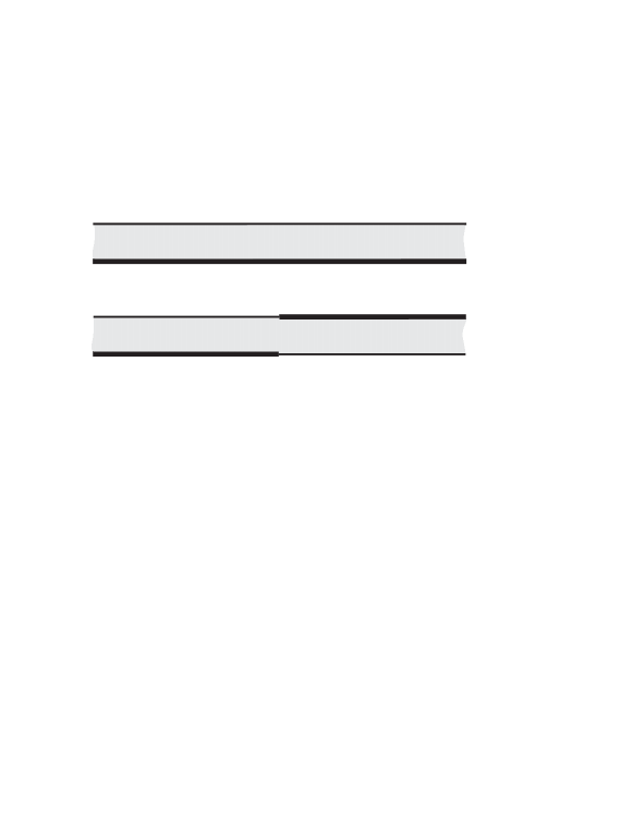
Figure 1: We consider the lower waveguide as a twist perturbation of the upper one, the twist being defined as a switch of Dirichlet (thick lines) to Neumann (thin lines) boundary conditions at one point, and vice versa.

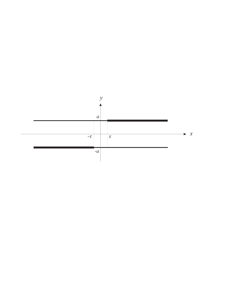
Figure 2: The geometry of our waveguide. The Dirichlet and Neumann boundary conditions are denoted by thick and thin lines, respectively.

The purpose of the present note is to demonstrate an analogous effect of twist in a two-dimensional waveguide with combined Dirichlet and Neumann boundary conditions. In this case the twist is represented by a switch of the boundary conditions at a given point, cf Figure 1. More precisely, given a real number $\varepsilon$ and a positive number $a$, let $-\Delta_{\varepsilon}$ be the Laplacian in the strip $\mathbb{R}\times(-a,a)$, subject to Dirichlet boundary conditions on $(-\infty,-\varepsilon)\times\{-a\}\cup(\varepsilon,+\infty)\times\{a\}$ and Neumann boundary conditions on $(-\varepsilon,+\infty)\times\{-a\}\cup(-\infty,\varepsilon)\times\{a\}$, cf Figure 2. It can be seen by a simple Neumann bracketing that the spectrum of $-\Delta_{\varepsilon}$ coincides with the interval $[\pi^{2}/(4a)^{2},+\infty)$ for all non-positive $\varepsilon$. Our main result shows that for $\varepsilon$ equal to zero the operator $-\Delta_{0}$ satisfies the following Hardy type inequality in the sense of quadratic forms:

$$-\Delta_{0}-\left(\frac{\pi}{4a}\right)^{2}\ \geq\ \rho(\cdot)\,,$$ (1)

where $\rho:\mathbb{R}\times(-a,a)\to\mathbb{R}$ is a positive function.

We would like to emphasize that in the situation where the boundary conditions are not exchanged – i.e. the Laplacian in $\mathbb{R}\times(-a,a)$ with uniform Dirichlet boundary conditions on one connected part of the boundary and Neumann boundary conditions on the other one, cf the upper waveguide in Figure 1 – the essential spectrum coincides with the essential spectrum of our waveguide, but the inequality (1) fails to hold for any non-trivial $\rho\geq 0$. The latter can be shown by a simple test-function argument. In other words, the switch of the boundary conditions creates a kind of repulsive perturbation represented by the function $\rho$. This leads to a certain stability of the spectrum similar to the one observed in [8]. In particular, it follows from (1) that the discrete spectrum remains empty after perturbing $-\Delta_{0}$ by a sufficiently small attractive perturbation.

One example of attractive perturbation is changing the boundary conditions by increasing the parameter $\varepsilon$, cf Figure 2. Due to the switch of the boundary conditions, the discrete eigenvalues do not appear for any positive $\varepsilon$, but only when $\varepsilon$ exceeds certain critical value $\varepsilon_{c}>0$. This effect was already observed by Dittrich and Kříž in [5]. Their result is obtained by a tedious decomposition of the Laplacian into the “transverse basis” and this also provides an estimate on the critical value $\varepsilon_{c}$ for which the eigenvalues emerge from the essential spectrum:

$$0.16\,a<\varepsilon_{c}<0.68\,a\,.$$ (2)

Since the proof of our Hardy inequality (1) can be easily carried over to the case when $\varepsilon$ is positive and small enough, we get as a byproduct of our method an alternative estimate on $\varepsilon_{c}$, too. The latter is worse than the one presented in [5], but on the other hand much simpler to obtain.

Finally, let us mention that Hardy inequalities for Schrödinger operators in two dimensions can be achieved by adding an appropriate local magnetic field to the system, too. This was first observed in [13] and later modified in [7] for Schrödinger operators in waveguides, cf also [1]. Curved waveguides in a homogeneous magnetic field have been recently studied in [15].

2 Main results and ideas

The Laplacian $-\Delta_{\varepsilon}$ is defined as the unique self-adjoint operator associated with the closure of the quadratic form $Q_{\varepsilon}$ defined in $L^{2}\big{(}\mathbb{R}\times(-a,a)\big{)}$ by

$$Q_{\varepsilon}[\psi]:=\int_{\mathbb{R}\times(-a,a)}\left(|\partial_{1}\psi(x,y)|^{2}+\partial_{2}\psi(x,y)|^{2}\right)dx\,dy$$ (3)

and by the domain $D(Q_{\varepsilon})$ which consists of restrictions to $\mathbb{R}\times(-a,a)$ of infinitely smooth functions with compact support in $\mathbb{R}^{2}$ and vanishing on the part of the boundary where the Dirichlet boundary conditions are imposed (cf [5] for more details). We are interested in the shifted quadratic form $\tilde{Q}_{\varepsilon}$ defined on the form domain $D(Q_{\varepsilon})$ by the prescription

$$\tilde{Q}_{\varepsilon}[\psi]:=Q[\psi]-\left(\frac{\pi}{4a}\right)^{2}\int_{\mathbb{R}\times(-a,a)}|\psi(x,y)|^{2}\,dx\,dy\,.$$ (4)

If $\varepsilon$ is negative, so that the opposite Dirichlet boundary conditions overlap, one can estimate the second term in (3) by the lowest eigenvalue of the Laplacian in the cross-section of length $2a$, subject to Dirichlet-Dirichlet or Dirichlet-Neumann boundary conditions. Neglecting the first term in (3), this immediately yields

$$-\Delta_{\varepsilon}-\left(\frac{\pi}{4a}\right)^{2}\ \geq\ 3\left(\frac{\pi}{4a}\right)^{2}\ \chi_{(\varepsilon,-\varepsilon)\times(-a,a)}(\cdot)\qquad\mbox{if}\qquad\varepsilon<0$$ (5)

in the sense of quadratic forms. Here $\chi_{M}$ denotes the characteristic function of a set $M$. The right hand side provides a non-negative Hardy weight in this case.

Of course, the trivial estimate leading to (5) is not useful for non-negative $\varepsilon$, in which case other methods have to be used. In this paper we get:

Theorem 1.

Given a real number $\varepsilon$ and a positive number $a$, let $-\Delta_{\varepsilon}$ be the Laplacian in the strip $\mathbb{R}\times(-a,a)$, subject to Dirichlet boundary conditions on $(-\infty,-\varepsilon)\times\{-a\}\cup(\varepsilon,+\infty)\times\{a\}$ and Neumann boundary conditions on $(-\varepsilon,+\infty)\times\{-a\}\cup(-\infty,\varepsilon)\times\{a\}$.

• There exists a positive constant $c$ such that the inequality

  $$-\Delta_{0}-\left(\frac{\pi}{4a}\right)^{2}\ \geq\ c\,\chi_{\omega}(\cdot)$$ (6)

  holds in the sense of quadratic forms. Here $\omega\supseteq(-a,a)\times(-a,a)$ and

  $$c\geq s_{1}\left(\frac{\pi}{4a}\right)^{2},$$

  where $s_{1}$ is the smallest root of the equation

  $$\sqrt{1-s}\ \tanh\left(\frac{\pi\,\sqrt{1-s}}{2\sqrt{2}}\right)=\sqrt{1/2+s}\ \tan\left(\frac{\pi\,\sqrt{1/2+s}}{2\sqrt{2}}\right).$$ (7)

• There exists a positive constant $\varepsilon_{c}\geq t_{1}\;\!a$ such that

  $$\sigma(-\Delta_{\varepsilon})=\big{[}\pi^{2}/(4a)^{2},\infty\big{)}$$

  for all $\varepsilon\leq\varepsilon_{c}$. Here $t_{1}$ is the smallest positive root of the equation

  $$\tanh\left(\frac{\pi\,(1-t)}{2\sqrt{2}}\right)=\sqrt{1/2}\ \tan\left(\frac{\pi\,(1+t)}{2\sqrt{2}}\right).$$ (8)

The first result, i.e. the Hardy inequality for $-\Delta_{0}$, is new. On the other hand, a positive lower bound on $\varepsilon_{c}$ has already been established in [5], cf (2). In [5] the authors also find the numerical value $\varepsilon_{c}\approx 0.52\,a$. We have $s_{1}\approx 0.039$ and $t_{1}\approx 0.061$, and these numbers cannot be much improved by our method (cf the end of Section 4 for more details).

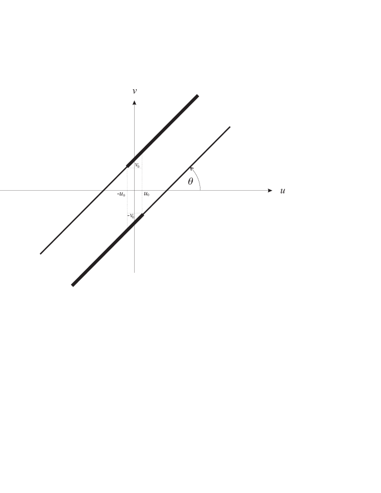
Figure 3: Rotating the Cartesian coordinate system by an appropriate angle $\theta$, one can employ the repulsive interaction due to the proximity of opposite Dirichlet boundary conditions (thick lines).

Although the effect which causes (6) is very similar to the twist studied in [8], the methods used in the respective proofs are completely different. The reason is that in our case the twist represents a singular deformation in the sense that it is discontinuous and occurs at one point only. Our main idea to prove Theorem 1 is to introduce rotated Cartesian coordinates in which one can employ the repulsive interaction due to the proximity of opposite Dirichlet boundary conditions, cf Figure 3. This is done in Section 3 where the initial problem is reduced to an ordinary differential equation. The latter is then investigated in Section 4 by standard methods for one-dimensional Schrödinger operators.

Note that Theorem 1 contains a weaker version of inequality (1), namely with a compactly supported Hardy weight. However, (1) can be easily deduced from it:

Corollary 1.

Inequality (1) holds true with the function $\rho$ given by

$$\rho(x,y):=\frac{c_{h}}{1+x^{2}}\,,\qquad c_{h}:=\left(\max\big{\{}16,c^{-1}(2+16/a^{2})\big{\}}\right)^{-1}\,,$$

where $c$ is the constant from Theorem 1.

A short proof of Corollary 1, based on the classical one-dimensional Hardy inequality, is given in the concluding Section 5.

3 Reduction to a one-dimensional problem

Hereafter we consider non-negative $\varepsilon$ only. Let $(x,y)\in\mathbb{R}\times(-a,a)$. We introduce rotated Cartesian coordinates $(u,v)$ by the change of variables

$$(x,y)=f(u,v):=\big{(}u\cos\theta+v\sin\theta,-u\sin\theta+v\cos\theta\big{)}\,,$$ (9)

where $\theta\in(0,\pi/2)$. Clearly, the mapping $f:\Omega\to\mathbb{R}\times(-a,a)$ is a diffeomorphism with the preimage

$$\Omega:=f^{-1}(\mathbb{R}\times I) =\left\{(u,v)\in\mathbb{R}^{2}\,|\ u_{-}(v)<u<u_{+}(v)\right\}$$

$$=\left\{(u,v)\in\mathbb{R}^{2}\,|\ v_{-}(u)<v<v_{+}(u)\right\}\,,$$

where

$$u_{\pm}(v):=\frac{\pm a+v\cos\theta}{\sin\theta}\,,\qquad v_{\pm}(u):=\frac{\pm a+u\sin\theta}{\cos\theta}\,.$$

Introducing the (unitary) change of trial function $\psi\mapsto\psi\circ f:=\phi$ into the functional (3), we find

$$Q_{\varepsilon}[\phi\circ f^{-1}]=\int_{\Omega}\left(|\partial_{1}\phi(u,v)|^{2}+\partial_{2}\phi(u,v)|^{2}\right)du\,dv\,.$$ (10)

From the formulae

$$\phi\big{(}u,v_{\pm}(u)\big{)}=\psi\left(\frac{u\pm a\sin\theta}{\cos\theta},\pm a\right),\qquad\phi\big{(}u_{\pm}(v),v\big{)}=\psi\left(\frac{v\pm a\cos\theta}{\sin\theta},\mp a\right),$$

we observe the two following properties, respectively. First, $v\mapsto\phi(u,v)$ with $u$ fixed satisfies Dirichlet boundary conditions at both boundary points $v_{\pm}(u)$ if, and only if,

$$|u|<u_{0}:=a\sin\theta-\varepsilon\cos\theta\,;$$ (11)

otherwise it satisfies a combination of Dirichlet and (generalized) Neumann boundary conditions. Second, $u\mapsto\phi(u,v)$ with $v$ fixed satisfies a combination of Dirichlet and (generalized) Neumann boundary conditions, if, and only if,

$$|v|>v_{0}:=a\cos\theta+\varepsilon\sin\theta\,;$$ (12)

otherwise it satisfies (generalized) Neumann boundary conditions (i.e. none). While $v_{0}$ is positive by definition, we need to assume that

$$\varepsilon<a\,\tan\theta$$ (13)

in order to ensure the positivity of $u_{0}$.

We proceed by estimating the form (10) as follows. We estimate the second term in (10) by the lowest eigenvalue of the Laplacian in the cross-section of length $v_{+}(u)-v_{-}(u)=2a/\cos\theta$, subject to the boundary conditions of the type that $v\mapsto\phi(u,v)$ satisfies. We also estimate the first term in (10) by the lowest eigenvalue of the Laplacian in the cross-section of length $u_{+}(v)-u_{-}(v)=2a/\sin\theta$, subject to the boundary conditions of the type that $u\mapsto\phi(u,v)$ satisfies, but only in the subset of $\Omega$ where $|u|>u_{0}$ and $|v|>v_{0}$. That is,

$$\tilde{Q}_{\varepsilon}[\phi\circ f^{-1}]\geq\int_{\Omega_{1}\cup\Omega_{2}}|\partial_{1}\phi|^{2}+q_{+}\int_{\Omega_{1}}|\phi|^{2}-q_{-}\int_{\Omega_{2}}|\phi|^{2}\,,$$ (14)

where

$$\Omega_{1}:=\left\{(u,v)\in\Omega\,|\ |u|<u_{0}\right\}\,,\qquad\Omega_{2}:=\left\{(u,v)\in\Omega\,|\ |v|<v_{0},\ |u|>u_{0}\right\}\,,$$

and

$$q_{+}:=\left(\frac{\pi}{4a}\right)^{2}(4\cos^{2}\theta-1)\,,\qquad q_{-}:=\left(\frac{\pi}{4a}\right)^{2}\sin^{2}\theta\,.$$ (15)

Hereafter we further restrict the angle $\theta$ by the requirement

$$\theta\in(0,\pi/3)\,,$$ (16)

so that the term $q_{+}$ is positive.

We use the intermediate bound (14) as the starting point of the reduction to a one-dimensional problem. Let us introduce the disjoint sets

$$\Omega_{1}^{\prime}:=\left\{(u,v)\in\Omega\,|\ |u|<u_{0},\ |v|>v_{0}\right\}\,,\qquad\Omega_{2}^{\prime}:=\left\{(u,v)\in\Omega\,|\ |v|<v_{0}\right\}\,,$$

and note that the inclusions $\Omega_{1}^{\prime}\subset\Omega_{1}$ and $\Omega_{2}^{\prime}\subset\Omega_{1}\cup\Omega_{2}$ hold. Consequently, under the assumption (16), (14) implies the cruder bound

$$\tilde{Q}_{\varepsilon}[\phi\circ f^{-1}]\geq q_{+}\int_{\Omega_{1}^{\prime}}|\phi(u,v)|^{2}\,du\,dv+\int_{\Omega_{2}^{\prime}}\lambda(v)\,|\phi(u,v)|^{2}\,du\,dv\,,$$ (17)

where $\lambda(v)\in(q_{-},q_{+})$ is the lowest eigenvalue of the one-dimensional Neumann Schrödinger operator with the step-like potential

$$V(u,v):=q_{+}\ \chi_{(-u_{0},u_{0})}(u)-q_{-}\ \chi_{(u_{-}(v),-u_{0})\cup(u_{0},u_{+}(v))}(u)\,.$$

More precisely,

$$\lambda(v):=\inf_{\varphi}\frac{\int_{u_{-}(v)}^{u_{+}(v)}\Big{[}|\varphi^{\prime}(u)|^{2}+V(u,v)\,|\varphi(u)|^{2}\Big{]}\,du}{\int_{u_{-}(v)}^{u_{+}(v)}|\varphi(u)|^{2}\,du}\,,$$ (18)

where the infimum is taken over all non-zero functions from the Sobolev space $W^{1,2}\big{(}u_{-}(v),u_{+}(v)\big{)}$.

The formula (17) together with (18) transfers the initial two-dimensional problem into the study of an ordinary differential equation. That is, it remains to investigate the function $v\mapsto\lambda(v)$.

4 Study of the one-dimensional problem

First of all, we observe that $v\mapsto\lambda(v)$ is an even function with values in the open interval $(q_{-},q_{+})$ due to (16). Furthermore, its minimum is attained at the boundary points $v=\pm v_{0}$:

Lemma 1.

One has ${\displaystyle\inf_{v\in(-v_{0},v_{0})}\lambda(v)=\lambda(v_{0})\,.}$

Proof.

Let $h$, $l$ and $\delta$ be positive numbers such that $\delta<l$. For any real $c$, we consider the one-dimensional Schrödinger operator

$$H_{c}:=-\Delta+h\,\chi_{(c,c+\delta l)}\qquad\qquad\mbox{in}\qquad L^{2}\big{(}(0,l)\big{)}\,,$$

subject to Neumann boundary conditions. ($H_{c}$ is introduced in a standard way through the associated quadratic form defined in $W^{1,2}((0,l))$.) Let us show that

$$\forall c\in(0,l-\delta l),\qquad\inf\sigma(H_{c})\geq\inf\sigma(H_{0})\,,$$ (19)

which is equivalent to the statement of the Lemma.

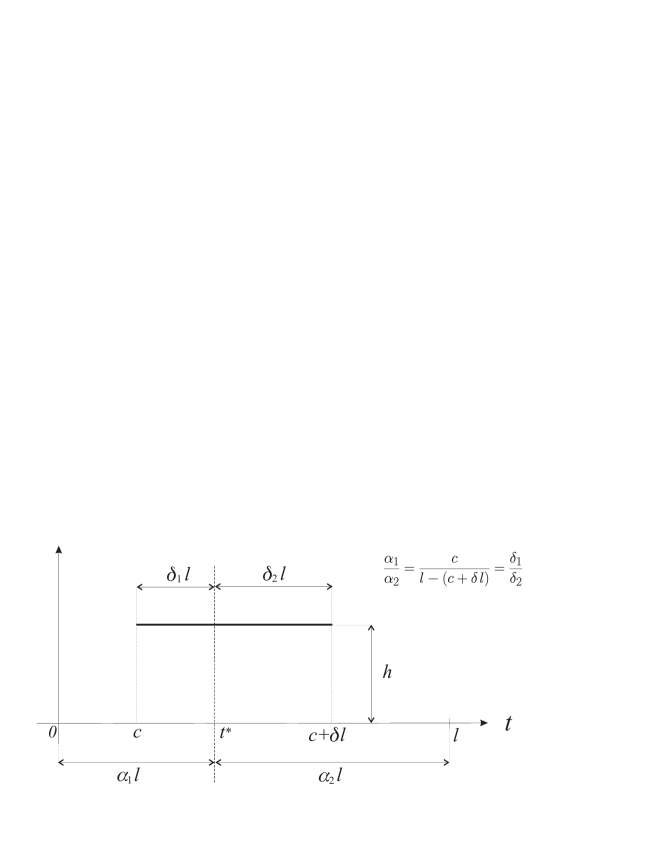
Figure 4: The construction used in the proof of Lemma 1.

The reader is advised to consult Figure 4 for the following construction. Given $c\in(0,l-\delta l)$, we find $\alpha_{1},\alpha_{2}\in(0,1)$ such that

$$\alpha_{1}+\alpha_{2}=1\qquad\mbox{and}\qquad\frac{\alpha_{1}}{\alpha_{2}}=\frac{c}{l-(c+\delta l)}\,.$$

We also define parameters $\delta_{1},\delta_{2}\in(0,\delta)$ by the equations

$$\delta_{1}+\delta_{2}=\delta\qquad\mbox{and}\qquad\frac{\delta_{1}}{\delta_{2}}=\frac{\alpha_{1}}{\alpha_{2}}\,.$$

It follows that $\alpha_{1}\;\!l=c+\delta_{1}l$. Let $t^{*}:=\alpha_{1}\;\!l\in(0,l)$.

The minimax principle yields

$$\inf\sigma(H_{c})\geq\inf\sigma(H_{c}^{N})\,,$$

where $H_{c}^{N}$ is the operator obtained from $H_{c}$ by imposing an additional Neumann boundary condition at the point $t^{*}$. $H_{c}^{N}$ is a direct sum of two operators, which are unitarily equivalent to

$$T_{1} :=-\Delta+h\,\chi_{(0,\delta_{1}l)} \qquad L^{2}\big{(}(0,\alpha_{1}\;\!l)\big{)}\,,$$ in

$$T_{2} :=-\Delta+h\,\chi_{(0,\delta_{2}l)} \qquad L^{2}\big{(}(0,\alpha_{2}\;\!l)\big{)}\,,$$ in

respectively, both subject to Neumann boundary conditions. Hence,

$$\sigma(H^{N}_{c})=\sigma(T_{1})\cup\sigma(T_{2})\,.$$ (20)

Obvious changes of variable show that that $T_{1}$ and $T_{2}$ are unitarily equivalent to the operators

$$\hat{T}_{1} :=-(\delta/\delta_{1})^{2}\,\Delta+h\,\chi_{(0,\delta l)} \qquad L^{2}\big{(}(0,l)\big{)}\,,$$ in

$$\hat{T}_{2} :=-(\delta/\delta_{2})^{2}\,\Delta+h\,\chi_{(0,\delta l)} \qquad L^{2}\big{(}(0,l)\big{)}\,,$$ in

respectively, both subject to Neumann boundary conditions. Consequently,

$$\hat{T}_{1}\geq H_{0}\qquad\mbox{and}\qquad\hat{T}_{2}\geq H_{0}$$

in the sense of quadratic forms. This together with (20) implies (19). ∎

As a consequence of (17) and the above Lemma, we therefore obtain

$$\tilde{Q}_{\varepsilon}[\phi\circ f^{-1}]\geq\lambda(v_{0})\int_{\Omega_{1}^{\prime}\cup\Omega_{2}^{\prime}}|\phi(u,v)|^{2}\,du\,dv\,.$$ (21)

We now turn to a more quantitative study of $\lambda(v_{0})$. The eigenvalue problem associated with (18) can be solved explicitly in the intervals where the potential $V$ is constant. Matching these solutions in the discontinuity points of $V$, one easily finds that $\lambda(v_{0})$ coincides with the smallest root $\lambda\in(q_{-},q_{+})$ of the equation

$$g_{1}(\lambda,\varepsilon,\theta)=g_{2}(\lambda,\varepsilon,\theta)\,,$$ (22)

where

$$g_{1}(\lambda,\varepsilon,\theta) :=\sqrt{q_{+}-\lambda}\ \tanh\left(2u_{0}\sqrt{q_{+}-\lambda}\right),$$

$$g_{2}(\lambda,\varepsilon,\theta) :=\sqrt{q_{-}+\lambda}\ \tan\left(2v_{0}\cot\theta\,\sqrt{q_{-}+\lambda}\right).$$

Recall that $q_{+},q_{-}$ and $u_{0},v_{0}$ are introduced in (15) and (11)–(12), respectively. Of course, $g_{2}$ is not defined for all the values of the parameters $\lambda,\varepsilon,\theta$, and we should rather multiply (22) by $\cos\big{(}2v_{0}\cot\theta\sqrt{q_{-}+\lambda}\big{)}$, but the resulting (regular) equation cannot be satisfied if the cosine equals zero, so we can leave (22) in the present form.

Let us first consider the case $\varepsilon=0$. A necessary condition to guarantee the eligibility of our method to prove Theorem 1 is that $\lambda(v_{0})$ is positive for certain angle $\theta$ satisfying (16). A numerical study of (22) shows that $\lambda(v_{0})$ achieves its maximum, given approximately by $0.040\,\pi^{2}/(4a)^{2}$, for the angle $\theta\approx 0.774$. Observing that the optimal angle is close to $\pi/4\approx 0.785$, let us fix henceforth:

$$\theta=\pi/4\,.$$ (23)

Since $\lambda\mapsto g_{1}(\lambda,0,\pi/4)$ is decreasing and continuous, $\lambda\mapsto g_{2}(\lambda,0,\pi/4)$ is increasing and continuous, and at $\lambda=0$ we have

$$\frac{g_{1}(0,0,\pi/4)}{g_{2}(0,0,\pi/4)}=\sqrt{2}\,\tanh\big{(}\sqrt{2}\,\pi/4\big{)}>1\,,$$ (24)

it follows that $\lambda(v_{0})$ is indeed positive for the choice (23). As for the numerical value, it is straightforward to check that (22) reduces to (7) and we find that the smallest root $s_{1}$ of the latter equals approximately $0.039$. Summing up, (21) implies

$$\tilde{Q}_{\varepsilon}[\phi\circ f^{-1}]\geq s_{1}\left(\frac{\pi}{4a}\right)^{2}\int_{\Omega_{1}^{\prime}\cup\Omega_{2}^{\prime}}|\phi(u,v)|^{2}\,du\,dv\,,$$

provided the angle $\theta$ is chosen according to (23). In order to establish (i) of Theorem 1, it remains to realize that

$$\overline{f\big{(}\Omega_{1}^{\prime}\cup\Omega_{2}^{\prime}\big{)}}\supset(-a,a)\times(-a,a)\,,$$

where $f$ is given by (9).

In the case of positive $\varepsilon$, we put $\lambda$ equal to zero in (22) and look for the smallest positive $\varepsilon$ satisfying the equation (22). This root satisfies the restriction (13) because $\varepsilon\mapsto g_{1}(0,\varepsilon,\pi/4)$ is decreasing and continuous, $\varepsilon\mapsto g_{2}(0,\varepsilon,\pi/4)$ is increasing and continuous, $g_{1}(0,a,\pi/4)=0$, $g_{2}(0,\varepsilon,\pi/4)$ tends to $+\infty$ as $\varepsilon\to a$, and we have (24) for $\varepsilon=0$. It is straightforward to check that (22) reduces to (8) for the choice (23) and the smallest positive root $t_{1}$ of the latter equals approximately $0.061$. Again, a more detailed numerical study of (22) shows that the best result reachable by the present method gives $\varepsilon_{c}\approx 0.063\,a$ with the optimal angle $\theta\approx 0.759$.

This concludes the proof of Theorem 1.

5 Proof of Corollary 1

The local Hardy inequality (6) is equivalent to

$$\int_{(-a,a)\times(-a,a)}|\psi|^{2}\leq\int_{\mathbb{R}\times(-a,a)}|\partial_{1}\psi|^{2}+\int_{\mathbb{R}\times(-a,a)}|\partial_{2}\psi|^{2}-\left(\frac{\pi}{4a}\right)^{2}\int_{\mathbb{R}\times(-a,a)}|\psi|^{2}$$

for any $\psi\in\overline{D(Q_{\varepsilon})}\subset W^{1,2}\big{(}\mathbb{R}\times(-a,a)\big{)}$. Here the sum of the last two terms on the right hand side is non-negative due to the boundary conditions that $\psi$ satisfies. Consequently, Corollary 1 follows at once by means of the following Hardy-type inequality for a Schrödinger operator in a strip with the potential being a characteristic function:

Lemma 2.

For any $\psi\in W^{1,2}\big{(}\mathbb{R}\times(-a,a)\big{)}$,

$$\int_{\mathbb{R}\times(-a,a)}w^{-2}\,|\psi|^{2}\ \leq\ 16\int_{\mathbb{R}\times(-a,a)}|\partial_{1}\psi|^{2}+\big{(}2+64/|J|^{2}\big{)}\int_{J\times(-a,a)}|\psi|^{2}\,,$$

where $w(x,y):=\sqrt{1+(x-x_{0})^{2}}$, $J$ is any bounded subinterval of $\mathbb{R}$ and $x_{0}$ is the mid-point of $J$.

This Lemma can be established quite easily by means of the classical one-dimensional Hardy inequality $\int_{\mathbb{R}}x^{-2}|v(x)|^{2}\,dx\leq 4\int_{\mathbb{R}}\,|v^{\prime}(x)|^{2}\,dx$ valid for any $v\in W^{1,2}(\mathbb{R})$ with $v(0)=0$ and Fubini’s theorem; we refer the reader to [8, Sec. 3.3] or [11, proof of Lem. 2] for more details.

References

• [1] D. Borisov, T. Ekholm, and H. Kovařík, Spectrum of the magnetic Schrödinger operator in a waveguide with combined boundary conditions, Ann. H. Poincaré 6 (2005), 327–342.
• [2] D. Borisov, P. Exner, R. Gadyl’shin, and D. Krejčiřík, Bound states in weakly deformed strips and layers, Ann. H. Poincaré 2 (2002), 553–572.
• [3] W. Bulla, F. Gesztesy, W. Renger, and B. Simon, Weakly coupled bound states in quantum waveguides, Proc. Amer. Math. Soc. 125 (1997), 1487–1495.
• [4] B. Chenaud, P. Duclos, P. Freitas, and D. Krejčiřík, Geometrically induced discrete spectrum in curved tubes, Differential Geom. Appl. 23 (2005), no. 2, 95–105.
• [5] J. Dittrich and J. Kříž, Bound states in straight quantum waveguides with combined boundary condition, J. Math. Phys. 43 (2002), 3892–3915.
• [6] P. Duclos and P. Exner, Curvature-induced bound states in quantum waveguides in two and three dimensions, Rev. Math. Phys. 7 (1995), 73–102.
• [7] T. Ekholm and H. Kovařík, Stability of the magnetic Schrödinger operator in a waveguide, Comm. in PDE 30 (2005), 539–565.
• [8] T. Ekholm, H. Kovařík, and D. Krejčiřík, A Hardy inequality in twisted waveguides, submitted; preprint on [math-ph/0512050] (2005).
• [9] P. Exner and P. Šeba, Bound states in curved quantum waveguides, J. Math. Phys. 30 (1989), 2574–2580.
• [10] J. Goldstone and R. L. Jaffe, Bound states in twisting tubes, Phys. Rev. B 45 (1992), 14100–14107.
• [11] D. Krejčiřík, Hardy inequalities for strips on ruled surfaces, J. Inequal. Appl., to appear; preprint on [math.SP/0511257] (2005).
• [12] D. Krejčiřík and J. Kříž, On the spectrum of curved quantum waveguides, Publ. RIMS, Kyoto University 41 (2005), no. 3, 757–791.
• [13] A. Laptev and T. Weidl, Hardy inequalities for magnetic Dirichlet forms, Oper. Theory Adv. Appl. 108 (1999), 299–305.
• [14] J. T. Londergan, J. P. Carini, and D. P. Murdock, Binding and scattering in two-dimensional systems, LNP, vol. m60, Springer, Berlin, 1999.
• [15] O. Olendski and L. Mikhailovska, Curved quantum waveguides in uniform magnetic fields, Phys. Rev. B 72 (2005), 235314.
• [16] W. Renger and W. Bulla, Existence of bound states in quantum waveguides under weak conditions, Lett. Math. Phys. 35 (1995), 1–12.
Refer to caption