Abstract

The one-dimensional chain of coupled oscillators with long-range power-law interaction is considered. The equation of motion in the infrared limit are mapped onto the continuum equation with the Riesz fractional derivative of order $\alpha$, when $0<\alpha<2$. The evolution of soliton-like and breather-like structures are obtained numerically and compared for both types of simulations: using the chain of oscillators and using the continuous medium equation with the fractional derivative.

PACS: 45.05.+x; 45.50.-j; 45.10.Hj

Keywords: Long-range interaction, Fractional oscillator, Fractional equations

1 Introduction

Nowadays it become clear that anomalous dynamics and kinetics may be not so pathological as it was believed earlier. More and more situations has been reported in the literature supporting this [2, 3, 4, 7, 13]. The immediate causes for these anomalies could be attributed to fractal or multi-fractal character of phase space, Lèvy flights, dynamical traps, or long-range correlations which are present in many interesting applications [3, 4, 5, 6]. The desolated once fractional order calculus revives again in order to discribe such problems. Indeed, equations which involve derivatives or integrals of non-integer order appeared to be very successful in describing anomalous kinetics and transport [5, 7, 8, 9, 10, 11, 12, 13].

However, fractional equations could be rarely derived explicitly from the equations of motion or from a Hamiltonian of the model. More often fractional equations for dynamics or kinetics appear as some phenomenological models. Recently, the method to obtain fractional analogues of equations of motion was considered for the bunch of problems related to sets of coupled particles or other objects that interact via a power-like potential [14, 15]. Examples of such systems are one-dimensional chain of interacting oscillators, spins, or waves that can be considered as a benchmark for numerous applications in physics, chemistry, biology, etc. [17, 18, 19, 20, 21, 36, 43]. Transfer from the set of Hamiltonian equations to the continuous media equation with fractional derivatives is an approximate procedure. Its formal realization can be perfomed using the so-called ”transform operator” [15]. Different applications of the operator have already been used to derive fractional sine-Gordon and fractional Hilbert equation [14], to study synchronization of coupled oscillators [15], and for fractional Ginzburg-Landau equation [16].

Localized in space structures, such as solitons or breathers are the subjects of a great interest since a long time. These structures have been widely studied in discrete systems on lattices with different types of interactions as well as in their continuous analogues (for a review, see [35, 38]). Solitons in a one-dimensional lattice with the long-range Lennard-Jones-type interaction were considered in [39]. Kinks in the Frenkel-Kontorova model with long-range interparticle interactions were studied in [40]. The properties of time periodic spatially localized solutions (breathers) on discrete chains in the presence of algebraically decaying interactions were considered in [36] and recently in [37]. Energy and decay properties of discrete breathers in systems with long-range interactions have also been studied in the framework of the Klein-Gordon [38], and discrete nonlinear Schrodinger equations [41]. A remarkable property of the dynamics described by the equation with fractional space derivatives is that the soliton or breather type solutions have power-like tails. Similar features were observed in the prototype lattice models with power-like long-range interactions [36, 37, 43, 44, 45]. As it was shown in [15, 16], analysis of the equations with fractional derivatives (FD) can provide fairly quickly results for the space asymptotics of their solutions. Replacement of the system of particles with power long-range interactions by an equation with FD will be called fractional equation approximation (FEA). As it was shown in [15, 16], the FEA appears in the infrared limit when the wave number $k\rightarrow 0$ and some other conditions that will be derived later. At the same time, in many applied problems equations with FD can appear as an intrinsic feature of the system (see examples in reviews [3, 10]). Integration of equations with FD needs specific algorithms which are fairly time consuming with not yet well defined errors [47].

The goal of this paper is to study a duality of Hamiltonian dynamics of system of particles with power-like interactions with the solutions of equations with FD using the transform operator. As a model to be studied we consider a chain of interacting oscillators that can be described by the sine-Gordon equation in the continuous limit.

To incorporate long-range interparticle interactions several nonlocal generalizations of the sine-Gordon equation were considered in Refs. [43, 44, 45] using the integro-differential equations of motion. The generalization of the standard sine-Gordon equation with space FD was proposed and numerically studied in [42]. The form of the fractional Sine-Gordon equation was $u_{tt}-{}^{R}D^{\alpha}u+\sin u=0$, where ${}^{R}D^{\alpha}$ is the Riesz space fractional derivative, $1<\alpha<2$. This equation was proposed as an interpolation between the classical sine-Gordon equation and a nonlocal sine-Gordon equation. Here, we consider the one-dimentional lattice of coupled non-linear oscillators. We focus on the dynamics of soliton-like and breather-like patterns. Following [14], we make the transform to the infrared limit and derive the fractional sine-Gordon equation which describes the dynamics of the lattice. Using both, Hamiltonian lattice dynamics and the fractional sine-Gordon (FSD) equation, we can compare solutions and demonstrate their similarity as well as to discuss conditions when such duality is applicable.

The obtained results can be used in a twofold way: firstly, we show how the infrared limit for the chain of oscillators can be described by the corresponding FSG equation with similar solutions; secondly, we propose the replacement of the integration scheme of equations with FD by the system of coupled Hamiltonian equations. The latter can be considered as a new way of analysis of the equations with FD.

2 Long-range interaction of oscillators

Consider a one-dimensional system of interacting oscillators described by the Hamiltonian

$$H=\sum_{n=-\infty}^{+\infty}\left[\frac{M}{2}\;\dot{u}_{n}^{2}+\frac{J_{0}}{2}\sum_{\begin{subarray}{c}m=-\infty\\ n\neq m\end{subarray}}^{+\infty}\;\frac{1}{|n-m|^{1+\alpha}}\;u_{n}u_{m}+\frac{J_{1}}{2}\;u_{n}^{2}+J_{2}\left(1-\cos\left(\frac{2\pi u_{n}}{a}\right)\right)\right],$$ (1)

where $M$ is mass and $u_{n}$ is displacement from the equilibrium. The last two terms characterize an interaction of the chain with the external on-site potential which is defined by the periodic function with period $a$ and amplitude $J_{2}$. The second term in Eq. (1) takes into account the interaction of the oscillators in the chain. Here, we consider nonlocal coupling given by the power-law function. Constant $\alpha$ is a physical relevant parameter. Some integer values of $\alpha$ corresponds to the well-known physical situations: Coulomb potential corresponds to $\alpha=0$, dipole-dipole interaction corresponds to $\alpha=2$, and the limit $\alpha\rightarrow\infty$ is for the case of nearest-neighbor interaction.

From Hamiltonian (1) it follows the equation of motion,

$$\frac{\partial^{2}u_{n}}{\partial t^{2}}+J_{0}\sum_{\begin{subarray}{c}m=-\infty\\ n\neq m\end{subarray}}^{+\infty}\;\frac{1}{|n-m|^{1+\alpha}}\;u_{m}+J_{1}u_{n}+J_{2}\sin\left(u_{n}\right)=0,$$ (2)

where we put $M=1$ and the period $a=2\pi$.

Let us sketch the derivation of continuous medium equation. We define the field $\hat{u}(k,t)$ on $[-K/2,K/2]$ as

$$\hat{u}(k,t)=\sum_{n=-\infty}^{+\infty}\;u_{n}(t)\;e^{-ikx_{n}}={\cal F}_{\Delta}\{u_{n}(t)\},$$ (3)

where $x_{n}=n\Delta x$, and $\Delta x=2\pi/K$ is distance between oscillators

$$u_{n}(t)=\frac{1}{K}\int_{-K/2}^{+K/2}dk\ \hat{u}(k,t)\;e^{ikx_{n}}={\cal F}^{-1}_{\Delta}\{\hat{u}(k,t)\}.$$ (4)

These equations are the basis for the Fourier transform which is obtained by transforming $u_{n}(t)=u(n\Delta x,t)$ from discrete variable $x_{n}=n\Delta x$ to a continuous one in the limit as $\Delta x\rightarrow 0$ ($K\rightarrow\infty$). The Fourier transform is a generalization of (3), (4) in the limit as $\Delta x\rightarrow 0$. Replace the discrete $u_{n}(t)$ with continuous $u(x,t)$ while letting $x_{n}=n\Delta x=2\pi n/K\rightarrow x$. Then change the sum to an integral, and Eqs. (3), (4) become

$$\tilde{u}(k,t)=\int^{+\infty}_{-\infty}dx\ e^{-ikx}u(x,t)={\cal F}\{u(x,t)\},$$ (5)

$$u(x,t)=\frac{1}{2\pi}\int^{+\infty}_{-\infty}dk\ e^{ikx}\tilde{u}(k,t)={\cal F}^{-1}\{\tilde{u}(k,t)\},$$ (6)

where

$$\tilde{u}(k,t)={\cal L}\hat{u}(k,t),\quad u(x,t)={\cal L}u_{n}(t),\quad u_{n}(t)=u(x_{n},t),$$ (7)

and ${\cal L}$ denotes the passage to the limit $\Delta x\rightarrow 0$ ($K\rightarrow\infty$). The procedure of the replacement of a discrete model by the continuous one is defined by the following operations:
1) The Fourier series transform:

$${\cal F}_{\Delta}:\quad u_{n}(t)\rightarrow{\cal F}_{\Delta}\{u_{n}(t)\}=\hat{u}(k,t);$$ (8)

2) The passage to the limit $\Delta x\rightarrow 0$:

$${\cal L}:\quad\hat{u}(k,t)\rightarrow{\cal L}\{\hat{u}(k,t)\}=\tilde{u}(k,t);$$ (9)

3) The inverse Fourier transform:

$${\cal F}^{-1}:\quad\tilde{u}(k,t)\rightarrow{\cal F}^{-1}\{\tilde{u}(k,t)\}=u(x,t).$$ (10)

The operation $T={\cal F}^{-1}{\cal L}\ {\cal F}_{\Delta}$ can be called a transform operation (transform map), since it performs a tranfrormation of a discrete model of coupled oscillators by the continuous medium model. In a similar to [14, 15] way, we can obtain from (2) the equation for $\hat{u}(k,t)$ using (3)

$$\frac{\partial^{2}\hat{u}(k,t)}{\partial t^{2}}+J_{0}\;\hat{J}_{\alpha}(k)\;\hat{u}(k,t)+J_{1}\;\hat{u}(k,t)+J_{2}\;\mathcal{F}_{\Delta}\{\sin\left(u_{n}(t)\right)\}=0,$$ (11)

where

$$\hat{J}_{\alpha}(k)=\sum_{\begin{subarray}{c}n=-\infty\\ n\neq 0\end{subarray}}^{+\infty}e^{-ikn\Delta x}\frac{1}{|n|^{1+\alpha}}=\sum^{+\infty}_{n=1}\frac{1}{n^{1+\alpha}}\left(e^{-ikn\Delta x}+e^{ikn\Delta x}\right)=Li_{1+\alpha}(e^{ik\Delta x})+Li_{1+\alpha}(e^{-ik\Delta x}),$$ (12)

and $Li_{1+\alpha}(z)$ is a polylogarithm function. Using the series representation of the polylogarithm [46]

$$Li_{\beta}(e^{z})=\Gamma(1-\beta)(-z)^{\beta-1}+\sum^{\infty}_{n=0}\frac{\zeta(\beta-n)}{n!}z^{n},\quad|z|<2\pi,\;\;\beta\not=1,2,3...,$$ (13)

we obtain

$$\hat{J}_{\alpha}(k)=a_{\alpha}\;|\Delta x|^{\alpha}\;|k|^{\alpha}+2\sum^{\infty}_{n=0}\frac{\zeta(1+\alpha-2n)}{(2n)!}(\Delta x)^{2n}(-k^{2})^{n},\quad|k|<1,\quad\alpha\not=0,1,2,3...,$$ (14)

where $J_{\alpha}(0)=2\zeta(1+\alpha)$, $\zeta$ is the Riemann zeta-function and

$$a_{\alpha}=2\;\Gamma(-\alpha)\;\cos\left(\frac{\pi\alpha}{2}\right).$$ (15)

Function $\hat{J}_{\alpha}(k)$ can also be presented in the form

$$\hat{J}_{\alpha}(k)=2\sum^{\infty}_{n=1}\frac{\cos(kn\Delta x)}{n^{1+\alpha}},$$ (16)

from which it follows that

$$\hat{J}_{\alpha}(k+2\pi m/\Delta x)=\hat{J}_{\alpha}(k),$$ (17)

where $m$ is an integer. For $\alpha=2$, $\hat{J}_{\alpha}(k)$ is the Clausen function $Cl_{2}(k)$ [33].

Combinig all expressions, Eq. (11) takes the form

$$\frac{\partial^{2}\hat{u}(k,t)}{\partial t^{2}}+J_{0}\;a_{\alpha}|\Delta x|^{\alpha}\;|k|^{\alpha}\;\hat{u}(k,t)+2J_{0}\sum^{\infty}_{n=0}\frac{\zeta(\alpha+1-2n)}{(2n)!}(\Delta x)^{2n}(-k^{2})^{n}\hat{u}(k,t)+$$ (18)

$$+J_{1}\;\hat{u}(k,t)+J_{2}\;\mathcal{F}_{\Delta}\{\sin\left(u_{n}(t)\right)\}=0.$$

We will be interested in the limit $\Delta k\rightarrow 0$. Then the Eq. (18) can be written in a simplified way

$$\frac{\partial^{2}}{\partial t^{2}}\hat{u}(k,t)+\bar{J}_{0}\;\hat{\mathcal{T}}_{\alpha,\Delta}(k)\;\hat{u}(k,t)+J_{1}\;\hat{u}(k,t)+J_{2}\;\mathcal{F}_{\Delta}\{\sin\left(u_{n}(t)\right)\}=0,\quad\alpha\not=0,1,2,...,$$ (19)

where $\bar{J}_{0}=J_{0}|\Delta x|^{min\{\alpha,2\}}$ and

$$\hat{\mathcal{T}}_{\alpha,\Delta}(k)=\begin{cases}a_{\alpha}|k|^{\alpha}-|\Delta x|^{2-\alpha}\zeta(\alpha-1)k^{2},&0<\alpha<2,\quad(\alpha\not=1)\cr|\Delta x|^{\alpha-2}a_{\alpha}|k|^{\alpha}-\zeta(\alpha-1)k^{2},&2<\alpha<4,\quad(\alpha\not=3).\end{cases}$$ (20)

The expression (20) was obtained in [14, 15] in a slightly different way. Let us note that (20) has a crossover scale for

$$k_{0}=|a_{\alpha}/\zeta(\alpha-1)|^{1/(2-\alpha)}|\Delta x|^{-1}$$ (21)

such that $\hat{\mathcal{T}}_{\alpha,\Delta}(k)\sim k^{2}$ for $\alpha>2$, $k\ll k_{0}$ and nontrivial expression $\hat{\mathcal{T}}_{\alpha,\Delta}(k)\sim|k|^{\alpha}$ appears only for $\alpha<2$, $k\ll k_{0}$. The crossover was considered also in [15, 27]. The expression for $\hat{\mathcal{T}}_{\alpha,\Delta}(k)$ can be considered as a Fourier transform of the operator

$$\mathcal{T}_{\alpha,n}\;u_{n}(t)\equiv\sum_{\begin{subarray}{c}m=-\infty\\ m\neq n\end{subarray}}^{+\infty}\;|n-m|^{-(1+\alpha)}\;u_{m}(t).$$ (22)

Performing the transition to the limit $k\ll k_{0}$ (or more precisely $k\Delta x\ll k_{0}\Delta x$), and applying inverse Fourier transform to (19) gives

$$\frac{\partial^{2}}{\partial t^{2}}u(x,t)+\bar{J}_{0}\;\mathcal{T}_{\alpha}(x)\;u(x,t)+J_{1}\;u(x,t)+J_{2}\;\sin\left(u(x,t)\right)=0\quad\alpha\not=0,1,2,...,$$ (23)

where

$$\mathcal{T}_{\alpha}(x)=\mathcal{F}^{-1}\{\hat{\mathcal{T}}_{\alpha}(k)\}=\begin{cases}-a_{\alpha}\frac{\partial^{\alpha}}{\partial|x|^{\alpha}},&0<\alpha<2,\quad(\alpha\not=1)\cr\zeta(\alpha-1)\frac{\partial^{2}}{\partial|x|^{2}},&2<\alpha<4,\quad(\alpha\not=3);\end{cases}$$ (24)

$$\hat{\mathcal{T}}_{\alpha}(k)=\begin{cases}a_{\alpha}|k|^{\alpha},&0<\alpha<2,\quad(\alpha\not=1)\cr-\zeta(\alpha-1)\;k^{2},&2<\alpha<4,\quad(\alpha\not=3).\end{cases}$$

Here, we have used the connection between the Riesz fractional derivative and its Fourier transform [29]:

$$|k|^{\alpha}\longleftrightarrow-\frac{\partial^{\alpha}}{\partial|x|^{\alpha}},\quad k^{2}\longleftrightarrow-\frac{\partial^{2}}{\partial|x|^{2}}.$$ (25)

The properties of the Riesz derivative can be found in [29, 30, 31, 32].

If we consider a system with Hamiltonian $H=H_{1}+H_{int}$, where

$$H_{1}=\sum_{n=-\infty}^{+\infty}\left[\frac{1}{2}\;\dot{u}_{n}^{2}+\;V(u_{n})\right],\quad H_{int}=\frac{1}{2}J_{0}\sum_{\begin{subarray}{c}n,m=-\infty\\ n\neq m\end{subarray}}^{+\infty}\frac{1}{|n-m|^{1+\alpha}}\;g(u_{n})\;g(u_{m}),$$ (26)

where $g(u)$ is some function of $u$. Equation (1) appears for $g(u)=u$. The corresponding generalization of (23) is easily obtained as

$$\frac{\partial^{2}u(x,t)}{\partial t^{2}}=V^{\prime}(u(x,t))+\bar{J}_{0}\;g^{\prime}(u(x,t))\mathcal{T}_{\alpha}(x)\;g(u(x,t)),\;\;\;(\alpha\not=0,1,2,...),$$ (27)

where $g^{\prime}(u)=\partial g(u)/\partial u$ and $\hat{\mathcal{T}_{\alpha}}(x)$ is the same as in (24).

3 Numerical methods

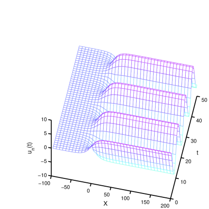
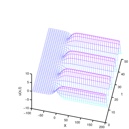
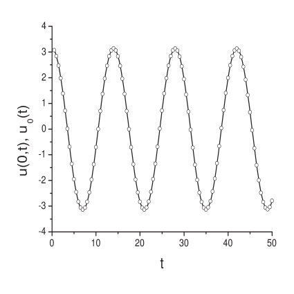
Figure 1: Kink-like structures obtained from the evolution of the system of coupled oscillators (left panel) and from the solution of the FSG equation (right panel). Bottom panel: Comparison of the time evolution of the central oscillator $u_{0}(t)$ (solid curve) with the time evolution of the $u(0,t)$ (circles) obtained from the solution of the FSG equation. Exponent $\alpha=1.21$.

We consider $N+1$ equally spaced by $\Delta x=2L/(N+1)$ coupled oscillators on the finite interval $(-L,L)$. The system is described by the equations of motion

$$\frac{\partial^{2}u_{n}}{\partial t^{2}}+J_{0}\sum_{\begin{subarray}{c}m=-N/2\\ m\neq n\end{subarray}}^{N/2}\;\frac{1}{|n-m|^{1+\alpha}}\;u_{m}+J_{1}u_{n}+J_{2}\sin u_{n}=0,\;\;(n=-\frac{N}{2},...,0,...,\frac{N}{2})$$ (28)

and $N$ is even. For $N\rightarrow\infty$ Eq. (28) coincides with Eq. (2). Specifing appropriate initial and boundary conditions, Eqs. (28) could be solved numerically for example by the discretization scheme or with the Runge-Kutta method.

For numerical solutions of the fractional sine-Gordon equation (23) with $0<\alpha<2$

$$\frac{\partial^{2}}{\partial t^{2}}u(x,t)-\bar{J}_{0}\;a_{\alpha}\frac{\partial^{\alpha}}{\partial|x|^{\alpha}}u(x,t)+J_{1}\;u(x,t)+J_{2}\;\sin\left(u(x,t)\right)=0,$$ (29)

we have used two methods which are described as the following.

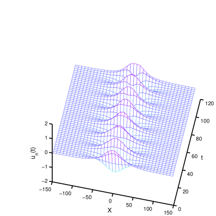
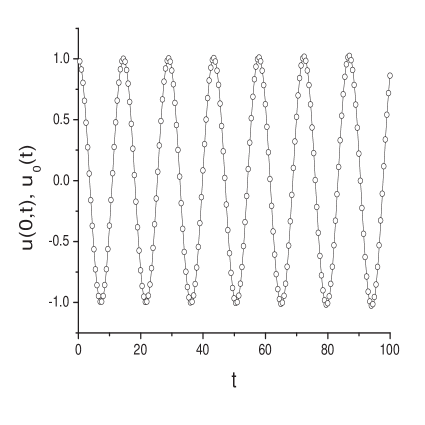
Figure 2: Left panel: Breather-like structures obtained from the evolution of the system of coupled oscillators. Right panel: solution of the FSG equation. Bottom figure: Comparison of the time evolution of the central oscillator $u_{0}(t)$ (solid curve) with the time evolution of the $u(0,t)$ (circles) obtained from the solution of the FSG equation. Exponent $\alpha=1.21$.

Method (a): The Riesz derivative could be represented as [48]

$$\frac{\partial^{\alpha}}{\partial|x|^{\alpha}}u(x,t)=-\frac{1}{2\cos(\pi\alpha/2)}\left({\cal D}^{\alpha}_{+}u(x,t)+{\cal D}^{\alpha}_{-}u(x,t)\right),$$ (30)

where ${\cal D}^{\alpha}_{\pm}$ are Riemann-Liouville left and right fractional derivatives defined by [29, 30, 31, 32]

$${\cal D}^{\alpha}_{+}u(x,t)=\frac{1}{\Gamma(m-\alpha)}\frac{\partial^{m}}{\partial x^{m}}\int^{x}_{-\infty}\frac{u(\xi,t)d\xi}{(x-\xi)^{\alpha-m+1}},$$

$${\cal D}^{\alpha}_{-}u(x,t)=\frac{(-1)^{m}}{\Gamma(m-\alpha)}\frac{\partial^{m}}{\partial x^{m}}\int^{\infty}_{x}\frac{Z(\xi,t)d\xi}{(\xi-x)^{\alpha-m+1}},$$ (31)

where $m-1<\alpha<m$. Since we seek for a numerical solution on a finite interval, we will also use the Riemann-Liouville left and right fractional derivatives defined on a finite interval $(-L,L)$

$${}_{-L}{\cal D}^{\alpha}_{x}u(x,t)=\frac{1}{\Gamma(m-\alpha)}\frac{\partial^{m}}{\partial x^{m}}\int^{x}_{-L}\frac{u(\xi,t)d\xi}{(x-\xi)^{\alpha-m+1}},$$

$${}_{x}{\cal D}^{\alpha}_{L}u(x,t)=\frac{(-1)^{m}}{\Gamma(m-\alpha)}\frac{\partial^{m}}{\partial x^{m}}\int^{L}_{x}\frac{u(\xi,t)d\xi}{(\xi-x)^{\alpha-m+1}}.$$ (32)

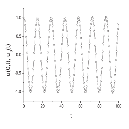
Figure 3: The same as in Fig. 1, but for $\alpha=1.51$.

As the next step we approximate the Riesz fractional derivative as follows

$$\frac{\partial^{\alpha}}{\partial|x|^{\alpha}}u(x,t)\simeq-\frac{1}{2\cos(\pi\alpha/2)}\left({}_{-L}{\cal D}^{\alpha}_{x}u(x,t)+{}_{x}{\cal D}^{\alpha}_{L}u(x,t)\right).$$ (33)

To compute Riemann-Liouville fractional derivatives we have used Grunwald-Letnikov discretization scheme [29]

$${}_{-L}{\cal D}^{\alpha}_{x}u(x,t)=\frac{1}{h^{\alpha}}\sum^{K_{-}}_{q=0}w_{k}\;u(x-qh,t),$$

$${}_{x}{\cal D}^{\alpha}_{L}u(x,t)=\frac{1}{h^{\alpha}}\sum^{K_{+}}_{q=0}w_{k}\;u(x+qh,t),$$ (34)

where $h$ is the discretization parameter, $K_{-}=\left[(x+L)/h\right]$, $K_{+}=\left[(L-x)/h\right]$, $[\nu]$ means integer part of $\nu$, and

$$w_{k}=\frac{\Gamma(q-\alpha)}{\Gamma(1+q)\;\Gamma(-\alpha)}.$$ (35)

However, for numerical calculations it is more convenient to use, instead of Eq. (35), the following recursion relation

$$w_{k}=\left(1-\frac{\alpha+1}{q}\right)\;w_{k-1},\;\;w_{0}=1.$$ (36)

The numerical scheme defined by the Eqs. (34) could be unstable. Therefore, to obtain a stable numerical scheme, one can use shifted Grunwald-Letnikov formulas proposed in [47]

$${}_{-L}{\cal D}^{\alpha}_{x}u(x,t)=\frac{1}{h^{\alpha}}\sum^{K_{-}}_{q=0}w_{k}\;u(x-(q-1)h,t).$$ (37)

$${}_{x}{\cal D}^{\alpha}_{L}u(x,t)=\frac{1}{h^{\alpha}}\sum^{K_{+}}_{q=0}w_{k}\;u(x+(q-1)h,t).$$

In our numerical simulations both numerical methods reproduce same results. To ensure the stability of the integration scheme the analog to the Courant-Friedrichs-Lewy stability condition should be fulfiled

$$\Delta t/(\Delta x)^{\alpha}<1/2.$$ (38)

After substitution of Eqs. (33), (34), (35) into Eq. (29), we have solved them using the explicit finite differences method for the second order time derivative

$$\frac{\partial^{2}}{\partial t^{2}}u(x,t)=\frac{u(x,t+\Delta t)+u(x,t-\Delta t)-2u(x,t)}{(\Delta t)^{2}}.$$ (39)

We have solved Eqs. (29) also by the forth order Runge-Kutta method in time. Results of both methods appear to be the same.

Method (b): The second method for numerical solution of the FSG equation is based on the fact that the Riesz space-fractional derivative admits the explicit representation in the form of an integral [29] with the limits of integration from zero to infinity. To use this definition for the solution of the equation on the finite interval we cut off the upper integration limit and approximate the Riesz derivative in the following way

$$\frac{\partial^{\alpha}}{\partial|x|^{\alpha}}u(x,t)\simeq\frac{\Gamma(1+\alpha)}{\pi}\sin\left(\frac{\alpha\pi}{2}\right)\int_{0}^{L}\frac{u(x+\eta,t)-2u(x,t)+u(x-\eta,t)}{\eta^{1+\alpha}}\;d\eta.$$ (40)

4 Numerical results

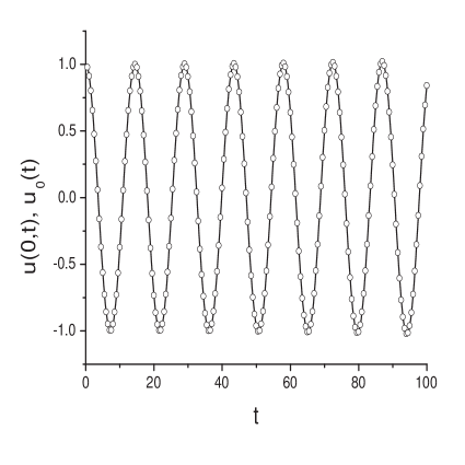
Figure 4: The same as in Fig. 1, but for $\alpha=1.91$.

In this section we compare numerical solutions obtained by two different ways: solution of equations of motion for the system of coupled oscillators starting from particular initial conditions and solution of FSG with the same initial conditions.

As the first kind of initial conditions we consider the topological soliton (kink) solution of the standard sine-Gordon equation

$$u_{n}(0)=4\arctan\left[\kappa\exp(x)\right],$$ (41)

where for the system of coupled oscillators the variable $x$ defines positions of oscillators, $x=n\Delta x$. The parameter $\kappa$ was fixed to $\kappa=0.001$. Three other constants in Eqs. (28) and (29) were $J_{1}=0.2,\;J_{0}=J_{2}=0.01$. The long-range interaction exponent is $\alpha=1.21$. We consider $N+1=1001$ equally spaced oscillators with the distance between them $\Delta x=2L/(N+1)$, $L=500$ and boundary conditions $u_{n+2L+1}(t)=u_{n}(t)+2\pi$. For the solution of FSG equation the discretization parameter $h$ was choosen to be $\Delta x/2$.

The time evolution of this initial function is shown in Fig. 1. The left panel represents the solution of the equations of motion for the discrete system of coupled oscillators, while the solution of the FSG equation is shown in the right panel. As it is seen from the figure, solutions of both systems are very similar to each other. On the bottom panel we compare the behaviour of $u_{0}(t)$ (solid line) and $u(0,t)$ (circles). The fractional order of the space derivative is reflected in the time oscillations of the initial soliton-like profile which is the exact stationary solution for the standard sine-Gordon equation with $\alpha=2$.

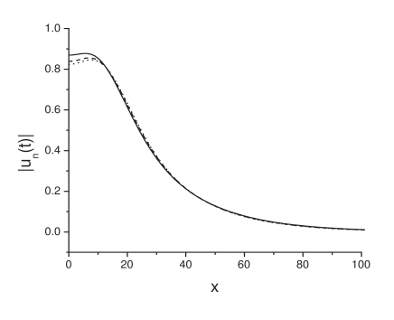
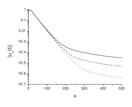
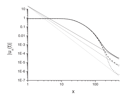
Figure 5: Profiles of the breather-like solutions obtained for the system of coupled oscillators for $t=100$ and $\alpha=1.21,1.51,1.91$ (solid, dashed and dotted curves respectively) in normal, the semi-logarithmic and in the double-logarithmic scales. Straight lines correspod to $f(x)\sim 1/x^{1+\alpha}$.

As a second kind of profile we consider two-parametric standing soliton solution of the standard sine-Gordon equation

$$u_{n}(0)=4\arctan\left[\frac{\nu}{\kappa\cosh(x)}\right],$$ (42)

where $\nu=1$ and $\kappa=0.05$. The constant was choosen such that the ratio wave length to the distance between oscillators is small. Three other constants in Eqs. (28), (29) were fixed to $J_{0}=0.01,\;J_{1}=J_{2}=0.1$. The number of oscillators $N+1=1001$, the distance between them $\Delta x=2L/(N+1)$ with $L=500$, and the periodic boundary conditions were applied $u_{n+2L+1}(t)=u_{n}(t)$. For the solution of the FSG equation the discretization we choose $h=\Delta x/2$.

Solutions of both equations appear in the form of a breather-like structures. They are ploted for different values of $\alpha$ in Figs. 2, 3 and 4. Solutions for the system of coupled oscillators are presented on the left panels of Fig. 2, 3 and 4, while solutions of the fractional sine-Gordon equation Eq. (29) are ploted on the right panels.

From these figures we conclude that in the infrared limit solutions of both systems are almost identical. Another conclution, that one can draw, is the low sensitivity of the core breather-like structure on the exponent $0<\alpha<2$. In Fig. 5 the snapshots of the breather-like solutions obtained for the same initial conditions are plotted for the time instant $t=100$. The long-range interaction mostly contributs to the behaviour of the tails of the breather-like solutions. The exponential spatial decay for short distances is modified by the power-law for large distances [36, 37] due to non-local interaction $\sim 1/x^{1+\alpha}$. In Fig. 5 (middle and low panels) the profiles of the breather-like solutions are ploted in semi-logarithmic and in double-logarithmic scales. The crossover from the exponential decay of the profile for a short distances to the power-law decay for a large distances is explicitly seen. With the increasing value of the parameter $\alpha$ the cross-over is shifted for longer time with the agreement to the reduction of the power-law interaction to the nearest-neighbor one for $\alpha\rightarrow\infty$. With a decrease of $\alpha$ the exponential part of the decay shrinks while the power-law decay is getting broad.

5 Conclusion

One-dimensional chain of classical interacting oscillators serve as a model for numerous applications in physics, chemistry, biology, etc. Long-range interactions, i.e., with forces proportional to $1/|x|^{1+\alpha}$ are important type of interaction for complex media. An interesting situation arrises when, for some reasons, the power $\alpha$ is non-integer. A remarkable feature of these interactions is the existence of a transform operator that replaces the set of coupled individual oscillator equations into the continuous medium equation with the space derivative of order $\alpha$, where $0<\alpha<2$, $\alpha\not=1$. Such transformation is an approximation and it appears in the infrared limit. This limit helps to consider different models and related phenomena in unified way applying different tools of fractional calculus.

Periodic space-localized oscillations which arise in discrete and continuous nonlinear systems have been widely studied in systems with short-range interactions. Here, the system with long-range interactions was considered. The method to map the set of equations of motion onto the continuos fractional order differential equation is developed in terms of the transform operator. It is known that the properties of a system with long-range interactions are very different from short-range one. The method offers a new tool for the analysis of different soliton- and breather-type solutions in such systems.

Vice versa, we hope that in some cases the obtained transform operator can be used to improve methods for numerical solutions of equations with fractional derivatives.

In quantum case the application of the transform operator would be highly interesting for example to a discrete nonlinear Schródinger-like equations with the power-law interactions.

References

- [1]
- [2] J.-P. Bouchaud, A. Georges, Phys. Rep. 195 (1990) 127-293.
- [3] G.M. Zaslavsky, Phys. Rep. 371 (2002) 461-580.
- [4] E.W. Montroll, M.F. Shlesinger, J. Lebowitz, E. Montroll (Eds.), North-Holland, Amsterdam, 1984, pp. 1-121.
- [5] A.I. Saichev, G.M. Zaslavsky, Chaos 7 (1997) 753-764.
- [6] V.V. Uchaikin, Physics-Uspekhi 46 (2003) 821-849; J. Exper. Theor. Phys. 97 (2003) 810-825.
- [7] M.F. Shlesinger, G.M. Zaslavsky, and J. Klafter, Nature (London) 263 (1993) 31-37.
- [8] J. Klafter, M.F. Shlesinger, G. Zumofen, Phys. Today 49 (1996) 32-39.
- [9] I.M. Sokolov, J. Klafter, A. Blumen, Phys. Today 55 (2002) 48-54.
- [10] R. Metzler, J. Klafter, Phys. Rep. 339 (2000) 1-77; J. Phys. A: Math. and Gen. 37 (2004) R161-R208.
- [11] J. Klafter, I.M. Sokolov, Phys. World 18 (2005) 29-32.
- [12] M.M. Meerschaert, D.A. Benson, B. Baeumer, Phys. Rev. E 63 (2001) 021112; Phys. Rev. E 59 (1999) 5026-5028.
- [13] R. Hilfer (Ed.), Applications of Fractional Calculus in Physics, World Scientific, Singapore, 2000.
- [14] N. Laskin, G.M. Zaslavsky, Submitted, E-print: nlin.SI/0512010 (2005).
- [15] V.E. Tarasov, G.M. Zaslavsky, Submitted, E-print: nlin.PS/0512013 (2005).
- [16] V.E. Tarasov, G.M. Zaslavsky, Physica A 354 (2005) 249-261.
- [17] F.J. Dyson, Commun. Math. Phys. 12 (1969) 91-107; Commun. Math. Phys. 12 (1969) 212-215; Commun. Math. Phys. 21 (1971) 269-283.
- [18] J. Frohlich, R. Israel, E.H. Lieb, B. Simon, Commum. Math. Phys. 62 (1978) 1-34.
- [19] S. Shima, Y. Kuramoto, Phys. Rev. E 69 (2004) 036213.
- [20] D. Mukamel, S. Ruffo, N. Schreiber, Phys. Rev. Lett. 95 (2005) 240604; J. Barre, F. Bouchet, T. Dauxois, S. Ruffo, J. Stat. Phys. 119 (2005) 677-713.
- [21] O.M. Braun, Y.S. Kivshar, Phys. Rep. 306 (1998) 2-108.
- [22] G.M. Zaslavsky, Physica D 76 (1994) 110-122.
- [23] G.M. Zaslavsky, M.A. Edelman, Physica D 193 (2004) 128-147.
- [24] B.A. Carreras, V.E. Lynch, G.M. Zaslavsky, Physics of Plasmas 8 (2001) 5096-5103.
- [25] V.V. Zosimov, L.M. Lyamshev, Uspekni Fizicheskih Nauk 165 (1995) 361-402.
- [26] R. Gorenflo, F. Mainardi, J. Comput. Appl. Math. 118 (2000) 283-299.
- [27] H. Weitzner, G.M. Zaslavsky, Commun. Nonlin. Sci. Numer. Simul. 8 (2003) 273-281.
- [28] A.V. Milovanov, J.J. Rasmussen, Phys. Lett. A 337 (2005) 75-80.
- [29] S.G. Samko, A.A. Kilbas, O.I. Marichev, Fractional Integrals and Derivatives Theory and Applications, Gordon and Breach, New York, 1993.
- [30] K.B. Oldham, J. Spanier, The Fractional Calculus, Academic Press, New York, 1974.
- [31] K.S. Miller, B. Ross, An Introduction to the Fractional Calculus and Fractional Differential Equations, Wiley, New York, 1993.
- [32] I. Podlubny, Fractional Differential Equations, Academic Press, New York, 1999.
- [33] L. Lewin, Polylogarithms and Associated Functions, North-Holland, New York, 1981.
- [34] V. Feller, An introduction to Probability Theory and its Applications, Vol. 2. Wiley, New York, 1971.
- [35] S. Flach, C.R. Willis, Phys. Rep. 295 (1998) 181-264.
- [36] S. Flach, Phys. Rev. E 58 (1998) R4116-R4119.
- [37] A. V. Gorbach, S. Flach, Phys. Rev. E 72 (2005) 056607.
- [38] O.M. Braun, Y.S. Kivshar, Phys. Rep. 306 (1998) 2-108.
- [39] Y. Ishimori, Prog. Theor. Phys. 68 (1982) 402-410.
- [40] O.M. Braun, Y.S. Kivshar, I.I Zelenskaya, Phys. Rev. B 41 (1990) 7118-7138.
- [41] Yu.B. Gaididei, S.F. Mingaleev, P.L. Christiansen, K.O. Rasmussen, Phys. Rev. E 55 (1997) 6141-6150; S.F. Mingaleev, Y.B. Gaididei, F.G. Mertens, Phys. Rev. E 58 (1998) 3833-3842.
- [42] G. Alfimov, T. Pierantozzi, L. Vazquez, in: Fractional differentiation and its applications, A. Le Mehautè, J.A. Tenreiro Machado, L.C. Trigeassou, J. Sabatier (Eds.), Proceedings of the IFAC-FDA’04 Workshop, Bordeaux, France, July 2004; pp. 153-162.
- [43] V.L. Pokrovsky, A. Virosztek, J. Phys. C 16 (1983) 4513-4525.
- [44] G.L. Alfimov, V.M. Eleonsky, L.M. Lerman, Chaos 8 (1998) 257-271.
- [45] G.L. Alfimov, V.G. Korolev, Phys. Lett. A 246 (1998) 429-435.
- [46] A. Erdèlyi, W. Magnus, F. Oberhettinger, F.G. Tricomi, Higher Transcendental Functions, Vol. 1. New York: Krieger, (1981) pp. 30-31.
- [47] M.M. Meerschaert, H.-P. Scheffler, C. Tadjeran, J. Comp. Phys. 211 (2006) 249-261.
- [48] R. Gorenflo and F. Mainardi, Feller fractional diffusion and Levy stable motions, in: Proceedings of the International Conference on ”Levy Processes: Theory and Applications”, Denmark, 18-22 January 1999, O.E. Barndorff-Nielsen, S.E. Graversen, T. Mikosch (Eds.), MPS-misc. 1999-11, pp. 11-122,