Fourier–Bessel functions of singular continuous measures and their many asymptotics

Abstract

We study the Fourier transform of polynomials in an orthogonal family, taken with respect to the orthogonality measure. Mastering the asymptotic properties of these transforms, that we call Fourier–Bessel functions, in the argument, the order, and in certain combinations of the two is required to solve a number of problems arising in quantum mechanics. We present known results, new approaches and open conjectures, hoping to justify our belief that the importance of these investigations extends beyond the application just mentioned, and may involve interesting discoveries.

1 Introduction and examples

Let $\mu$ be a positive measure, for which the moment problem is determined, and let $\{p_{n}(\mu;s)\}_{n\in{\bf N}}$ be its orthogonal polynomials. The Fourier-Bessel functions (F-B. for short) ${\cal J}_{n}(\mu;t)$ are the Fourier transforms of $p_{n}(\mu;s)$ with respect to $\mu$:

$${\cal J}_{n}(\mu;t):=\int d\mu(s)~{}p_{n}(\mu;s)~{}e^{-its}.$$ (1)

This nomenclature follows—for lack of better candidates—from the simple observation that when $\mu$ is the continuous measure with density $d\mu(s)=\frac{ds}{\pi\sqrt{1-s^{2}}}$, and therefore $p_{n}(\mu;s)$ are the (properly normalized) Chebyshev polynomials, the F-B. functions are the usual integer order Bessel functions: ${\cal J}_{n}(\mu;t)=(-i)^{n}J_{n}(t)$. When the measure is symmetrical with respect to the origin, as in this case, the F-B. functions are either real, or purely imaginary. A graph of the first few F-B. functions, multiplied by $i^{n}$, is displayed in Fig. 1 for a singular continuous measure supported on a real Julia set (to be introduced in the following). Notice the joyful oscillations that these F-B. functions feature, as opposed to the more disciplined, and in the end boring attitude of the $J_{n}$’s. This paper wants to be an ode to the fascinating properties of F-B. functions of singular continuous measures, that in my opinion are still largely unexplored: I shall present a few results, but mostly open problems. The style of this paper will be suggestive of possible developments, rather than assertive of formal results, and at times I shall gladly renounce to rigor in favor of intuition, hoping with confidence that others will take up where I have left, and complete the picture. In this way, I believe to be correctly interpreting Ed’s attitude towards mathematics as a communal endeavor, and it is not only a pleasure for me, but an honor, to dedicate to him these notes.

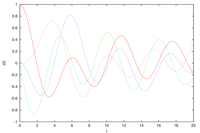
Fig. 1: F-B. functions $i^{n}{\cal J}_{n}(\mu;t)$, $n=0,1,2,3$, for a Julia set measure with $\lambda=2.9$. Different curves can be distinguished from the behavior at the origin: ${\cal J}_{n}(\mu;t)\sim t^{n}$, as in the Bessel case.

The asymptotic of F-B. functions for large values of the argument, $t$, is a classical theme of investigation, especially when $n=0$, since ${\cal J}_{0}(\mu;t)$ is the Fourier transform of the measure $\mu$ [1, 2, 3, 4, 5]. In this study, the nature of the orthogonality measure $\mu$ plays a major rôle. In fact, it is in the realm of singular, multi-fractal measures that the most interesting phenomena appear. First of all, at difference with the usual Bessel case, convergence of ${\cal J}_{n}(\mu;t)$ to zero is not to be expected, and indeed in Figure 2, that depicts a much larger argument range than Fig. 1, this time for a measure associated with a linear Iterated Function System, bursts of “activity” of ${\cal J}_{0}(\mu;t)$ are observed, amidst zones of quiescence. Because of similarities with the theory of turbulence, I have termed this phenomenon and its consequences quantum intermittency [6, 7, 8].

Fig. 2: F-B. function ${\cal J}_{0}(\mu;t)$ for an I.F.S. measure, over a larger $t$-scale than in Fig. (1).

A common technique to cope with these bursts is to take suitable time averages, like Cesaro’s. After averaging, decay of ${\cal J}_{n}(\mu;t)$ to zero actually takes place, according to an algebraic law. Now, two main problems can be investigated: the decay of the averaged F-B. functions themselves, and that of their (averaged) square moduli, this second problem having received larger attention than the first. In two recent papers [9, 10] we have collected known and new results on these questions, under the unifying theme of Mellin transforms. The following scheme is encountered in these theorems, under very broad hypotheses (typically, the existence of orthogonal polynomials): for any $x$ less than the divergence abscissa of a potential theoretic function, the Cesaro average of F-B. functions (or of their square moduli) decays faster than $t^{-x}$. The divergence abscissas entering these theorems are identified as the local dimension of the measure at zero in the first case, and as the correlation dimension of the measure in the second. The appearance of dimensional quantities of the orthogonality measure is not accidental: indeed, they play a major rôle in the asymptotics of F-B. functions, as it will become apparent in the following.

Quite different is the asymptotic behavior for large values of the order, and fixed argument. A general result can be obtained on the basis of a Chebyshev expansion of the matrix exponential [11]: this theorem states that under the sole hypothesis that the support of $\mu$ is bounded, at fixed time $t$, for any $\alpha\geq 0$, there exist a constant $C_{\alpha}$ so that the F-B. functions ${\cal J}_{n}(\mu;t)$ decay faster than exponentially in $n$:

$$|{\cal J}_{n}(\mu;t)|\leq C_{\alpha}e^{-\alpha n}\;\;\mbox{for all}\;n.$$ (2)

The need to refine this estimate will become apparent in Sect. 8.

So far we have described asymptotic questions of a quite conventional kinship. The best way to introduce and motivate the new questions that we would like to answer, is to outline a quantum mechanical interpretation of the F-B. functions. An alternative physical interpretation, that considers the propagation of excitations in chains of classical linear oscillators, can be found in [8].

Recall that the orthogonal polynomials $\{p_{n}(\mu;s)\}_{n\in{\bf N}}$ satisfy a recursion relation that can be written in vector form as

$$s\;{\bf p}(\mu;s)={\bf J}_{\mu}{\bf p}(\mu;s),$$ (3)

where ${\bf p}(\mu;s)$ is the infinite vector of orthogonal polynomials evaluated at position $s$, and ${\bf J}_{\mu}$ is the Jacobi matrix uniquely associated with $\mu$ (in the case when the moment problem is determined, of course). We can formally think of ${\bf J}_{\mu}$ as a self-adjoint operator acting in the space of square summable sequences, $l_{2}({\bf Z}_{+})$ (for the precise treatment of this part see [10]), and consider the evolution that it generates via Schrödinger equation:

$$i\frac{d}{dt}\psi(t)={\bf J}_{\mu}\psi(t).$$ (4)

In this equation, $\psi(t)$ is the wave-function, a vector that evolves in the space $l_{2}({\bf Z}_{+})$ and defines the state of the quantum system. At any time $t$, we can compute the projection of $\psi(t)$ on $e_{n}$, the $n$-th vector of the canonical basis of $l_{2}({\bf Z}_{+})$:

$$\psi_{n}(t):=(\psi(t),e_{n}),$$ (5)

where $(\cdot,\cdot)$ denotes the scalar product in $l_{2}({\bf Z}_{+})$.

The initial state of the evolution, $\psi(0)$, can be chosen freely. Letting it coincide with the first basis vector, $e_{0}$, leads to the conclusion [10] that $\psi_{n}(t)$, the projection of the time evolution on the $n$-th basis state, can be precisely identified with ${\cal J}_{n}(\mu;t)$, the $n$-th F-B. function:

$$\psi_{n}(t)={\cal J}_{n}(\mu;t).$$ (6)

The physical amplitudes of the quantum motion are the square moduli of the projections of the wave-function on the basis states of Hilbert space, $|\psi_{n}(t)|^{2}$. They are interpreted as the quantum probability to find the system in the state $e_{n}$ at the time $t$. As such, they can be used to define the expected values of dynamical operators. Unitarity of the quantum evolution operator, $e^{-it{\bf J}_{\mu}}$, implies the probability conservation formula

$$\sum_{n=0}^{\infty}|{\cal J}_{n}(\mu;t)|^{2}=1,$$ (7)

valid for all times $t$. This formula gives a new meaning to the analogous one already known for integer order Bessel functions.

Think now of $n$ as labelling the position in a regular one-dimensional lattice. Then, $\psi(0)=e_{0}$ describes a quantum system initially localized in the origin of this lattice, and consequently $|\psi_{n}(t)|^{2}$ describes the spreading of the quantum wave over this space. Figure 3 shows the initial part of the evolution in the case of the usual Bessel functions (for which the measure $\mu$ is absolutely continuous), and Figure 4 displays the same information in the case of a singular continuous Julia set measure. Differences between the two are apparent.

Fig. 3: F-B. functions $|{\cal J}_{n}(\mu;t)|^{2}$ versus time $t$ and space $n+1$, for $d\mu(s)=\frac{ds}{\pi\sqrt{1-s^{2}}}$.This, and all three–dimensional graphs are zoomable for better viewing.

Fig. 4: F-B. functions $|{\cal J}_{n}(\mu;t)|^{2}$ versus time $t$ and space $n+1$, for a Julia set measure with $\lambda=2.9$.

To gauge this spreading we utilize the moments of the position $n$,

$$\nu_{\alpha}(t):=\sum_{n=0}^{\infty}n^{\alpha}|\psi_{n}(t)|^{2}=\sum_{n=0}^{\infty}n^{\alpha}|{\cal J}_{n}(\mu;t)|^{2}.$$ (8)

Here, the index $\alpha$ takes all positive real values [12].

As it happens, for the singular measures that we are interested in, the asymptotic behavior of the position moments $\nu_{\alpha}(t)$ is power-law, with non–trivial exponents: we therefore define the growth exponents $\beta^{\pm}(\alpha)$ via the upper and lower limits

$$\beta^{\pm}(\alpha)=\frac{1}{\alpha}\lim_{t\rightarrow\infty}\mbox{$(\stackrel{{\scriptstyle sup}}{{\scriptstyle inf}})$}\frac{\log\nu_{\alpha}(t)}{\log t}.$$ (9)

The functions $\beta^{\pm}(\alpha)$ are also called the quantum intermittency functions.

In the setting so defined, trivially $\beta^{\pm}(\alpha)\leq 1$, and $\beta^{\pm}(\alpha)=1$ in the Bessel case. For singular measures, bounds related to dimensional characteristics become of importance [13]: under the sole request of existence of the orthogonal polynomials of $\mu$, it is proven that $\beta^{-}(\alpha)\geq\mbox{dim}_{H}(\mu),$ where $\mbox{dim}_{H}(\mu)$ is the Hausdorff dimension of $\mu$, and $\beta^{+}(\alpha)\geq\mbox{dim}_{p}(\mu),$ the last quantity being the packing (or Tricot) fractal dimension. Indeed, these theorems are even more general than required for our purpose: they apply to any quantum evolution in a separable Hilbert space, see the original references for details.

Notice that the above bounds do not depend upon the index $\alpha$. According to my definition, quantum intermittency is present when $\beta^{\pm}(\alpha)$ are not constant functions of the argument $\alpha$. However strange it might seem at first, this case is typical of singular continuous measures supported on Cantor sets. The name of the game of much recent theoretical research has therefore been to study these functions, and to track the origin of their behavior in the properties of the measure $\mu$, and of its orthogonal polynomials. This is the problem that will be discussed in this paper.

2 Kinematics, and expansion in orthogonal polynomials

The quantities described in the Introduction can be obviously expressed in terms of orthogonal polynomials. In fact, the position moments $\nu_{\alpha}(t)$ can be written as

$$\nu_{\alpha}(t)=\sum_{n=0}^{\infty}n^{\alpha}\int\!\!\int d\mu(s)d\mu(r)e^{i(r-s)t}p_{n}(\mu;s)p_{n}(\mu;r)\;.$$ (10)

We are therefore confronted with the highly singular kernel

$$K^{\alpha}_{\mu}(r,s):=\sum_{n=0}^{\infty}n^{\alpha}p_{n}(\mu;s)p_{n}(\mu;r).$$ (11)

When $\alpha=0$, we obtain the reproducing kernel of the orthogonal polynomials of $\mu$: $K^{0}_{\mu}(r,s)=\delta_{\mu}(r-s)$.

The behavior of individual F-B. functions can be rather erratic. The common procedure is then to perform a time average. Cesaro averaging is a common choice, but other forms of averaging work as well. For instance, Gaussian averaging,

$${\cal A}_{G}(f)(t):=\frac{1}{2t\sqrt{\pi}}\int_{-\infty}^{\infty}e^{-\frac{s^{2}}{t^{2}}}f(s)ds,$$ (12)

where $f$ is either $\nu_{\alpha}(t)$, or ${\cal J}_{n}(\mu;t)$, has the advantage of a better regularity in the windowing function: we have in fact

$${\cal A}_{G}(\nu_{\alpha})(t)=\sum_{n=0}^{\infty}n^{\alpha}\int\!\!\int d\mu(s)d\mu(r)\chi_{1/t}(r-s)p_{n}(\mu;s)p_{n}(\mu;r),\;$$ (13)

where $\chi_{\omega}(u)=e^{-\frac{u^{2}}{\omega^{2}}}$ is a smooth analogue of the characteristic function of the interval $[-\omega,\omega]$. For ease of notation, we use the convention $\omega:=t^{-1}$ throughout this paper.

3 Distribution functions and lower bounds to the growth exponents

In the study of the general problem (9) the consideration of a finite truncation of the $\alpha=0$ moment, turns out to be useful. Define

$$\nu_{0}(N,\omega):=\int\!\!\int d\mu(s)\,d\mu(r)\chi_{\omega}(r-s)\sum_{n=0}^{N}\,p_{n}(\mu;s)\,p_{n}(\mu;r)\;.$$ (14)

This is the Gaussian time average, up to time $t=\omega^{-1}$, of the sum of the squares of the first $N+1$ F-B. functions. Gaussian averaging is not as mandatory here as it is in the study of individual F-B. functions, since its regulating rôle can be also supplied by the summation over $n$, and yet I am not aware of any rigorous treatment involving only the Fourier kernel $\chi_{\omega}(r-s)=e^{-i(r-s)/\omega}$. In any case, we shall maintain this ambiguity offering theoretical results that require averaging, and—at times—experimental results showing that averaging can be disposed of.

In physical language, the discrete probability distribution $|\psi_{n}(t)|^{2}=|{\cal J}_{n}(\mu;t)|^{2}$ (recall the normalization condition Eq. (7)) is called the wave–packet, and therefore $\nu_{0}(N,\omega)$ is the distribution function of the Gaussian averaged wave–packet. It therefore contains all the information on this probability distribution, and a detailed control of this quantity, in $N$ and $\omega$, extends to the growth exponents.

Typically, upper bounds on $\nu_{0}(N,\omega)$ have been found, yielding lower bounds on growth exponents for positive $\alpha$. This can be easily seen by remembering that the quantum probability distribution $|\psi_{n}(t)|^{2}$ is normalized by eq. (7): $\lim_{N\rightarrow\infty}\nu_{0}(N,\omega)=1$ for all $\omega$; therefore, squeezing the head of the distribution fatten its tail. The original result is Guarneri’s inequality $\beta^{-}(\alpha)\geq D_{1}(\mu)$, extended by Combes [14] to many-dimensional Schrödinger operators, further refined by Guarneri and Schulz-Baldes [15], and by Tcheremchantsev et al. [16, 17] to a moment-dependent bound, in the form

$$\beta^{-}(\alpha)\geq D_{(1+\alpha)^{-1}}(\mu).$$ (15)

In the above, $D_{q}(\mu)$ are the generalized dimensions of the measure $\mu$, of index $q$, that we shall define in Sect. 5. The original hypothesis [15] that these dimensions exist for all $q\in{\bf R}$, and are finite for some $q<1$ has been weakened [17] to cover the case of the most general positive Borel measure $\mu$. Notice finally that these bounds involve generalized dimensions of positive index, between zero and one. Inspection of the proofs reveals that this is a limitation of the technique, that deals rather crudely with the role of the orthogonal polynomials $p_{n}(\mu;x)$.

4 Further lower bounds to the growth exponents

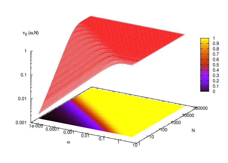
Fig. 5: Truncated, averaged moment $\nu_{0}(N,\omega)$ for a Julia set measure with $\lambda=2.9$. To the left of the figure, the region where the ansatz (16) is well verified. The flat plateau to the right, at $\nu_{0}(N,\omega)=1$, stretches over all values of $N$ that at time $t=\omega^{-1}$ have not yet been reached by the propagating wave.

An improvement of these estimates is obtained if one controls the growth rate of orthogonal polynomials. The first attempt in this direction has been the renormalization theory of orthogonal polynomials of IFS measures [7, 8] that we shall meet in the following. Successively, the imaginative formula for the function $\nu_{0}(N,\omega)$ proposed by Ketzmerick et al. [18] opened a different perspective:

$$\nu_{0}(N,\omega)\sim N^{d}\omega^{D_{2}(\mu)},$$ (16)

where $D_{2}(\mu)$ is the correlation dimension of the measure $\mu$ (see Sect. 5) and $d$ is a suitable constant that depends on properties of the orthogonal polynomials of $\mu$, as we shall discuss momentarily [19]. Formula (16) can obviously be valid only for $1\ll N\ll\omega^{-D_{2}(\mu)/d}$. It predicts a scaling form, both in time and space, of the wave–packet. Pictorially, the authors of [18] say that, at fixed time, the initial part of the wave-packet decays with $n$ as $n^{d-1}$. In Figure 5 the function $\nu_{0}(N,\omega)$ is plotted versus $\omega$ and $N$, in the case of Figs. 1 and 4. We observe that the scaling (16) is well verified, in the region in space–time that corresponds to the decay of excitations, behind the wave–front.

Starting from formula (16) Ketzmerick et al. have derived a lower bound to the growth exponents in the form $\beta(\alpha)\geq D_{2}(\mu)/d$. This result can be put on rigorous footing recalling the observation that the square moduli of all F-B. functions decay as $t^{-D_{2}(\mu)}$ [9]. Therefore $\nu_{0}(N,\omega)\,\omega^{-D_{2}(\mu)}$ is a bounded function of $\omega$. If in addition there exist $\gamma$ and $c$ larger than zero such that

$$\nu_{0}(N,\omega)\leq cN^{\gamma}\omega^{D_{2}(\mu)},$$ (17)

for all $N$ and $\omega$, we can conclude that

$$\beta_{-}(\alpha)\,\geq\,\frac{D_{2}(\mu)}{\gamma}\;,$$ (18)

for all positive values of $\alpha$. In Sect. 9 we shall comment on the effectiveness of this bound in an exactly computable situation. Notice that our definition of $\gamma$ over-estimates the parameter $d$ in Ketzmerick et al. surmise (16), and eq. (17) may be too crude of an estimate. Yet, in certain cases, numerical experiments as that of Fig. 5 show that in a region of space–time the surmise is a good description of the function $\nu_{0}(N,\omega)$, and $d$ is a good approximation of $\gamma$. As a matter of facts, the exponent $d$ has a dimensional flavor, which mixes the asymptotic properties of the orthogonal polynomials $p_{n}(\mu;s)$ and the local properties of the measure $\mu$. To see this, it is now time to briefly introduce the generalized dimensions of a measure $\mu$.

5 Generalized dimensions of the orthogonality measure

The spectrum of generalized dimensions $D_{q}(\mu)$ of a positive measure $\mu$ is given, for real $q\neq 1$, by the law

$$\int\!d\mu(r)(\mu(B_{\omega}(r)))^{q-1}\sim\omega^{(q-1)D_{q}(\mu)}.$$ (19)

The scaling law is made precise by taking superior and inferior limits, when $\omega$ tends to zero, of the logarithm of the l.h.s. integral over the logarithm of $\omega$. Of course, an appropriate formula exists also for $q=1$. A thorough study of generalized dimensions is to be found in [20], [21].

We mention now for future reference an alternative approach to the evaluation of the scaling law (19). Think of covering the support of $\mu$ by a family $\Sigma$ of disjoint intervals $I_{\sigma}$, of length $l_{\sigma}$, and measure $\pi_{\sigma}:=\mu(I_{\sigma})$. Then, $D_{q}(\mu)$ is defined as the divergence abscissa of $H(x,\Sigma)$,

$$H(x,\Sigma):=\sum_{\sigma\in\Sigma}\pi_{\sigma}^{q}\;l_{\sigma}^{(1-q)x},$$ (20)

when the generalized limit of finer and finer coverings is taken.

We can now understand why the correlation dimension have a rôle in our problem [22]. Let us start from the expansion

$${\cal A}_{G}(|{\cal J}_{n}(\mu;t)|^{2})=\int\!\!\int d\mu(s)d\mu(r)\chi_{\omega}(r-s)p_{n}(\mu;s)p_{n}(\mu;r),\;$$ (21)

and observe that, when $\omega\ll 1/n$, the variation of $p_{n}(\mu;s)$ over $B_{\omega}(r)$, the ball of radius $\omega$ centered at $r$, is negligible, so that $p_{n}(\mu;s)\simeq p_{n}(\mu;r)$ and

$${\cal A}_{G}(|{\cal J}_{n}(\mu;t)|^{2})\;\;\;\simeq\;\;\;\int\!d\mu(r)p_{n}^{2}(\mu;r)\!\int d\mu(s)\chi_{\omega}(r-s)\;\;\;\simeq\;\;\;\int\!d\mu(r)p_{n}^{2}(\mu;r)\mu(B_{\omega}(r)).$$ (22)

Now, the correlation dimension $D_{2}(\mu)$ is obtained setting $q=2$ in eq. (19). It so happens that the function $p_{n}^{2}(\mu;r)$ does not alter the asymptotic behavior of the last integral in eq. (22), and therefore $D_{2}(\mu)$ governs the asymptotic decay of the averaged square moduli of F-B. functions. Of course, this is not a substitute for a rigorous proof, that has been obtained in a variety of ways in the literature, as explained in detail in [9].

6 Asymptotics of the orthogonal polynomials and growth exponents

We can now return to the wave–propagation problem, and apply the same approximation as in eq. (22) to $\nu_{0}(N,\omega)$, to get

$$\nu_{0}(N,\omega)\simeq\int\!d\mu(r)\mu(B_{\omega}(r))\sum_{n=0}^{N}p_{n}^{2}(\mu;r).$$ (23)

Suppose now that the orthogonal polynomials verify a scaling relation of the kind

$$\sum_{n=0}^{N}p_{n}^{2}(\mu;r)\sim g(r)N^{d(r)},$$ (24)

for large $N$, with local dimension $d(r)$, and a smooth function $g(r)$ (where smooth is intended as a subleading behavior). Then one meets the problem, familiar in dimension theory, of determining the exponent $d(\omega)$, defined by

$$\int\!d\varrho_{\omega}(r)g(r)N^{d(r)}\sim N^{d(\omega)},$$ (25)

in terms of the measures $d\varrho_{\omega}(r):=\mu(B_{\omega}(r))d\mu(r)$. Suppose now that there exists constants $C$ and $\gamma$ such that

$$\sum_{n=0}^{N}p^{2}_{n}(\mu;x)\leq CN^{\gamma}$$ (26)

for any $x$ in the support of $\mu$, then Ketzmerick et al. surmise holds. A more refined analysis [15, 17] can be carried on restricting the integral with respect to $\mu$ to appropriate subsets $\Omega$ of the support of $\mu$, so to obtain lower bounds to $1-\nu_{0}(N,\omega)$. This analysis shows that indeed under the above hypothesis 26 the following lower bound holds:

$$\beta^{-}(\alpha)\geq\frac{1}{\gamma}D_{(1-\alpha/\gamma)}(\mu).$$ (27)

Two comments are in order: the first, is that eq. (27) is a better bound than $D_{2}(\mu)/\gamma$. The second, that generalized dimensions of argument less than one appear. We shall soon return to this fact.

In the same line is the local result [24]: suppose that there exists a Borel set $S$ of positive measure, so that the restriction of $\mu$ to this set is $a$-continuous (it gives zero weight to any set of null $a$-dimensional Hausdorff measure) and so that there exists $\gamma$ such that for any $x\in S$ (26) is verified, then

$$\beta^{-}(\alpha)\geq\frac{a}{\gamma}.$$ (28)

Further lower bounds are described in [23], [17].

7 Upper bounds to the quantum intermittency function

Lower bounds on $\nu_{0}(N,\omega)$ do not lead to upper bounds on $\beta(\alpha)$ [24], that are therefore much harder to find [8, 25, 26, 27], also because the strategy of restricting the consideration to a subset $\Omega$ of the support of $\mu$ is not sufficient here.

The last quoted reference describes a rather interesting situation that is worth presenting in some detail, also because the techniques on which it is based might find wider applicability. One starts from the Jacobi matrices ${\bf J}_{\theta,\eta}$ introduced in [28] and defined by

$$xp_{k}(x;\mu)=(V_{\eta}(k)+\theta\delta_{0,k})p_{k}(x;\mu)+p_{k-1}(x;\mu)+p_{k+1}(x;\mu)$$ (29)

labelled by the real parameters $\theta\in[\theta_{0},\theta_{1}]$, $0<\theta_{0}<\theta_{1}<\infty$ and $\eta\in(0,\infty)$. The structure of the recurrence relation renders ${\bf J}_{\theta,\eta}$ a discrete Schrödinger operator, with potential $V_{\eta}(k)$. This is chosen to be null, except on a set $B$ of selected barrier locations, $B=\{L_{n},n\in{\bf Z}^{+}\}$: $V_{\eta}(k)=\chi_{B}(k)\;k^{\eta}.$ The exponent $\eta$ links location and height of the barrier. The limit $\eta=\infty$ corresponds to a Dirichlet condition at each $L_{n}$, that clearly means no propagation and pure point spectrum. On the other hand, $\eta=0$ gives barriers of constant height, and generically absolutely continuous spectrum if these are sparse enough. Sparseness is a convenient request for analysis: assume that for some $a>1$ and all $n\in{\bf Z}$ $L_{n+1}\geq aL_{n}.$ Under these conditions one can prove [27] that for all $\alpha$, $0<\alpha\leq 2$, and almost all $\theta$ one has that

$$\beta^{-}(\alpha)\leq\frac{\alpha+1}{2\eta+\alpha+1},$$ (30)

while $\beta^{+}(\alpha)=1$: there is a part of the wave-packet that moves linearly in time (one says ballistically, in the usual jargon) while the main body follows at a slower pace. We refer to [27] for the detailed analysis and illustrative pictures.

8 Wave–front propagation: unsolved asymptotics

The previous sections have dealt with the shape of the wave–packet behind the wave–front. This implies that time, the argument of the F-B. functions, is much larger than space, the order. To complete the picture we must take into account what happens in the opposite limit, and, more importantly for our goals, in the region of the wave–front. This will explain our remark of Sect. 3, on the fact that lower bounds on $\nu_{0}(N,\omega)$ in the first region do not yield control of $\beta(\alpha)$.

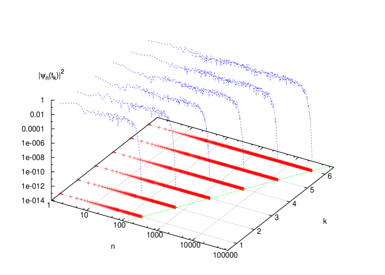
Fig. 6: Snapshots of $|\psi_{n}(t_{k})|^{2}$ at exponentially spaced times $t_{k}$, $k=1,\ldots,6$, versus $N$ and $k$ for an I.F.S. measure, described in Sect. 12. At the bottom of the graph, the fitting line for the wave–front indicates the law $n\sim t^{\eta}$, with $\eta=0.84165$.

A sequence of snapshots illustrating the wave-packet at exponentially spaced times is shown in Fig. 6. Over the time–span of the figure, the wave enlarges its size by more than two orders of magnitude. Two characteristics are to be remarked: the decay of the wave–packet is clearly consistent with eq. (2), but in addition it takes place rather abruptly past a wave–front position. The motion of this point, on the other hand, appears in Fig. 6 to follow an algebraic law, with exponent $\eta$. These two characteristics combined imply an upper bound to the growth exponents, $\beta^{+}(\alpha)\leq\eta$, for all positive values of $\alpha$.

In the usual Bessel case, it is well known that $\eta=1$ (Bessel functions decay abruptly when the order exceeds the exponent), and that the wave is propagating linearly, so that a speed of propagation can be defined. It is interesting to remark that Newton’s determination of the speed of sound ultimately relies on these properties [30],[8]. In the singular measure case, a speed cannot be defined, and we are forced to introduce the intermittency function $\beta$ of the moment order $\alpha$. In view of this, and of our previous remark on the difficulty of obtaining upper bounds to the growth exponents, it is of crucial relevance to develop techniques to control this particular asymptotics of the F-B. functions, so to enable us, for instance, to characterize the exponent $\eta$ observed in Fig. 6.

9 Julia Set Measures: renormalization equations

We now discuss an example that can be worked out exactly to a large extent. We choose for $\mu$ the balanced measure supported on a real Julia set, generated by the quadratic map $z\rightarrow z^{2}-\lambda$, for $\lambda\geq 2$ [31, 32]. The inverses of this map,

$$\phi_{j}(s)=j\;\sqrt{s+\lambda}$$ (31)

with $j=\pm 1$, can be seen as the non-linear maps of an Iterated Function System. The invariant measure of this I.F.S. is defined via the equation

$$\int f(x)d\mu(x)=\frac{1}{2}\sum_{j=\pm 1}\int(f\circ\phi_{j})(x)d\mu(x),$$ (32)

valid for any continuous function $f$. When $\lambda=2$, we obtain the orthogonality measure of the Chebyshev polynomials, suitably rescaled. When $\lambda>2$, the support of $\mu$ is a real Cantor set. In the graphs displayed in this paper, we have chosen $\lambda=2.9$ for no particular reason.

The hierarchical structure of the support of $\mu$ is brought to evidence by iterating the I.F.S. maps $k$ times: to keep the notation compact it is useful to define the index vector ${\bf\sigma}=(\sigma_{1},\ldots,\sigma_{k})$, with $\sigma_{i}\in\{+1,-1\}$, of length $|\sigma|=k$, and the associated composition maps $\phi_{\sigma}=\phi_{\sigma_{1}}\circ\phi_{\sigma_{2}}\circ\cdots\circ\phi_{\sigma_{k}}$. Let now $I_{\emptyset}$ be the convex hull of the support of the measure $\mu$, $I_{\emptyset}=[-\Lambda,\Lambda]$, where $\Lambda$ is the fixed point of $\phi_{+}$. At hierarchical order $k=|\sigma|$, the support of $\mu$ is covered by the intervals $I_{\sigma}$,

$$I_{\sigma}:=\phi_{\sigma}(I_{\emptyset}).$$ (33)

The following remarkable property holds for the orthogonal polynomials of this measure [33, 31]:

$$p_{2n}(\mu;\phi_{j}(s))=p_{n}(\mu;s),$$ (34)

for $j=\pm 1$. Applying this property, and the balance equation (32) to the Gaussian time averaged wave-function projections, ${\cal A}_{G}(|{\cal J}_{n}(\mu;t)|^{2})$, that we denote for short $\psi^{G}_{n}(t)$, we get:

$$\psi^{G}_{2n}(t)=\frac{1}{4}\sum_{\sigma,\sigma^{\prime}}\int\!\!\int d\mu(s)\,d\mu(r)\;\chi_{\omega}(\phi_{\sigma}(r)-\phi_{\sigma^{\prime}}(s))p_{n}(\mu;r)p_{n}(\mu;s).$$ (35)

Iterating the renormalization procedure $k$ times, we obtain the wave-function average projection at site $N=n2^{k}$, with $n$ and $k$ integers, in the form:

$$\psi^{G}_{N}(t)=\frac{1}{2^{2k}}\!\!\!\!\!\!\!\!\sum_{\scriptsize\begin{array}[]{c}\sigma,\sigma^{\prime}\\ |\sigma|=|\sigma^{\prime}|=k\end{array}}\!\!\!\!\!\!\!\!\int\!\!\int d\mu(s)\,d\mu(r)\;\chi_{\omega}(\phi_{\sigma}(r)-\phi_{\sigma^{\prime}}(s))\;p_{n}(\mu;r)p_{n}(\mu;s).$$ (36)

The non-diagonal contributions, $\sigma\neq\sigma^{\prime}$, in the balance equation (36) have a fast time decay and can be neglected. In addition, in the diagonal terms, the non-linear maps $\phi_{\sigma}$ can be replaced by a linearized version: for any $\sigma$, let now

$$l_{\sigma}(s):=\delta_{\sigma}s+\theta_{\sigma}$$ (37)

be the linear map, with coefficients $\delta_{\sigma}$ and $\theta_{\sigma}$, that takes $I_{\emptyset}$, the convex hull of the support of the measure $\mu$, exactly onto $I_{\sigma}$. In other words, $I_{\sigma}=\phi_{\sigma}(I_{\emptyset})=l_{\sigma}(I_{\emptyset})$, and the length of this cylinder is consequently proportional to $\delta_{\sigma}$: $|I_{\sigma}|=2\delta_{\sigma}\Lambda$. Usage of linear maps in the argument of $\chi_{\omega}$ has the effect of dividing $\omega$ by $\delta_{\sigma}$, so that

$$\psi^{G}_{N}(t)=\frac{1}{2^{2k}}\sum_{\sigma\mbox{\em\scriptsize s.t. }|\sigma|=k}\psi^{G}_{n}(t\delta_{\sigma})+{\cal E}(k,n,t),$$ (38)

where ${\cal E}(k,n,t)$ is the error involved in the approximations we have made. The related error estimates are rather involved, and aim to show that ${\cal E}(k,n,t)$ is negligible, in appropriate asymptotic expansions. We shall boldly do this in the following.

Eq. (38) is a renormalization equation, that links the wave-function projection at site $N$ and time $t$ to those at site $n$ and earlier times. As opposed to simple estimates of $\nu_{0}(\omega,N)$, this equation offers us a means of controlling the growth exponents. We have developed this idea in [7, 8] and in the more rigorous, yet less noticed ref. [34].

10 Julia set measures: analysis behind the wave front

We now employ the renormalization analysis, eq. (38), to compute exactly the behavior of $\nu_{0}(N,\omega)$ in the region behind the wave front:

$$\nu_{0}(N,\omega)\sim\sum_{j=0}^{n-1}2^{k}\psi^{G}_{j2^{k}}(\omega^{-1})\sim\sum_{\sigma\mbox{\em\scriptsize s.t. }|\sigma|=k}\sum_{j=0}^{n-1}\frac{1}{2^{k}}\psi^{G}_{j}(\delta_{\sigma}\omega^{-1})=\sum_{\sigma\mbox{\em\scriptsize s.t. }|\sigma|=k}\frac{1}{2^{k}}\nu_{0}(n,\omega/\delta_{\sigma}).$$ (39)

The form $\nu_{0}(N,\omega)\,\sim\,N^{\gamma}\;\omega^{\,D_{2}(\mu)}$ solves eq. (39); upon setting $\pi_{\sigma}:=2^{-k}$, we get

$$\sum_{\sigma\mbox{\em\scriptsize s.t. }|\sigma|=k}\pi_{\sigma}^{1+\gamma}\;\delta_{\sigma}^{-D_{2}(\mu)}\sim 1,$$ (40)

that implicitly determines $\gamma$. This determination is indeed transparent: comparing eq. (40) with the discrete evaluation of the generalized dimensions, eq. (20), we immediately obtain

$$D_{2}(\mu)\;=\;\gamma\;D_{1+\gamma}(\mu)\;,$$ (41)

and therefore

$$\gamma=1.$$ (42)

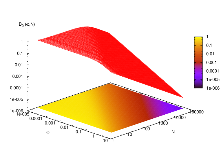
Fig. 7: $B_{0}(\omega,N):=N^{-1}\omega^{-D_{2}(\mu)}\nu_{0}(N,\omega)$ for the Julia set measure of Fig. 5.

Figure 7 shows the function $B_{0}(\omega,N):=N^{-1}\omega^{-D_{2}(\mu)}\nu_{0}(N,\omega)$, whose flat left piece confirms the validity of the scaling (16), and of the value $\gamma=1$.

According to Sect. 4, a consequence of this calculation is a lower bound on the positive exponents: $\beta(\alpha)\geq D_{2}(\mu)$. Notice that since $D_{2}(\mu)<D_{1}(\mu)$ this bound is weaker that the original Guarneri’s inequality $\beta(\alpha)\geq D_{1}(\mu)$ [35]. This fact is by no means accidental: information of the kind (16), and more general, on the $\nu_{0}(N,\omega)$ for small $N$ (with respect to an appropriate power of $\omega$) is not sufficient to control the growth exponents.

11 Surfing the Intermittent Quantum Wave

A treatment quite analogous to that of the previous section can be carried out for all truncated moments of order $\alpha>0$:

$$\nu_{\alpha}(N,\omega):=\sum_{n=0}^{N}n^{\alpha}{\cal A}_{G}(|{\cal J}_{n}(\mu;t)|^{2})=\int\!\!\int d\mu(s)\,d\mu(r)\chi_{\omega}(r-s)\sum_{n=0}^{N}\,n^{\alpha}p_{n}(\mu;s)\,p_{n}(\mu;r)\;.$$ (43)

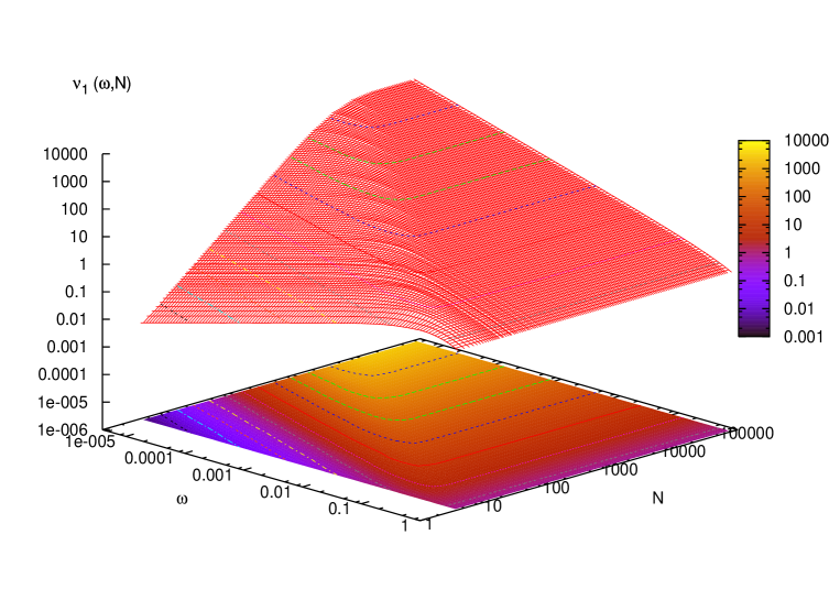
Fig. 8: Gaussian averaged, truncated first moment $\nu_{1}(\omega,N)$ for the Julia set measure with $\lambda=2.9$.

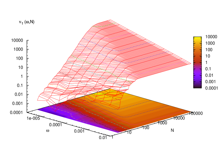
Fig. 9: Truncated first moment $\nu_{1}(\omega,N)$ for the Julia set measure with $\lambda=2.9$ without time–averaging. Notice the decay of fluctuations with increasing values of $N$.

Using the renormalization eq. (38) in the new situation leads to the result

$$\nu_{\alpha}(N,\omega)\,\sim\,N^{\gamma+\alpha}\;\omega^{\,D_{2}(\mu)},$$ (44)

valid in the regime of decaying F-B. functions, in the leftmost part of Fig. 8, where this behavior is clearly observed.

Notice that a new scaling region appears now to the right of the figure, ahead of the wave front, replacing the plateau that was obtained for $\alpha=0$: in fact, when the lattice site $N$ has not yet been reached by the wave, $\nu_{\alpha}(N,\omega)$ is independent of $N$, and is equal to the (Gaussian averaged) position moment of order $\alpha$. Therefore, in such region,

$$\nu_{\alpha}(N,\omega)\,\sim\,N^{0}\;\omega^{-\alpha\beta(\alpha)},$$ (45)

in which the intermittency function $\beta(\alpha)$ explicitly appears. Of course, this is a trivial observation. It can be turned into a constructive theory only if we can stretch our approximations to reach this region.

Pictorially, but appropriately, we can say that the lower bounds mentioned in the previous sections have been obtained by floating safely in the calm waters behind the wave–front. To the opposite, a complete theory of quantum intermittency can be obtained only if we are brave enough to catch the wave, boldly surfing on our approximation board the roaming waters of the F-B. wave–front, vividly depicted in Figure 4.

Achieving this goal is a rare accomplishment: the renormalization approach is the board that has enabled us to do this for Julia set measures [7, 8, 34]. First,

$$\nu_{\alpha}(t)\sim\sum_{j=0}^{\infty}2^{k}(j2^{k})^{\alpha}\psi^{G}_{j2^{k}}(t).$$ (46)

Then, employing again the renormalization eq. (36), we obtain

$$\nu_{\alpha}(t)\sim\sum_{\sigma\mbox{\em\scriptsize s.t. }|\sigma|=k}{2^{k(\alpha-1)}}\sum_{j=0}^{\infty}j^{\alpha}\psi^{G}_{j}(\delta_{\sigma}t)={2^{k(\alpha-1)}}\!\!\!\!\!\!\!\!\sum_{\sigma\mbox{\em\scriptsize s.t. }|\sigma|=k}\!\!\!\!\!\!\!\!\nu_{\alpha}(\delta_{\sigma}t)$$ (47)

This relation has the scaling solution $\nu_{\alpha}(t)\sim t^{\alpha\beta(\alpha)}$, whence by consistency

$$\sum_{\sigma\mbox{\em\scriptsize s.t. }|\sigma|=k}\pi_{\sigma}^{1-\alpha}\;\delta_{\sigma}^{\alpha\beta(\alpha)}\sim 1,$$ (48)

that unveils, by comparison with eq. (20), the fundamental Julia set relation

$$\beta(\alpha)\;=\;D_{1-\alpha}(\mu)\;,$$ (49)

that links growth exponents and generalized dimensions.

We have verified numerically that this relation holds exactly even without time–averaging [7, 8, 34]. Indeed, Fig. 9 displays the truncated, instantaneous value of the first moment versus $\omega$ and $N$: as we have remarked previously, summation over $n$ supplies the regularizing effect.

In [36] a relation formally written as eq. (49), but different in meaning, has been obtained by a renormalization procedure over Fibonacci Jacobi matrices. In such relation $\beta(\alpha)$ are the growth exponents of moments averaged over initial sites (which mathematically amounts to averaging over different Jacobi Hamiltonians), and $D_{q}$ are the thermodynamical dimensions of the logarithmic potential equilibrium measure, that we shall also consider in the next section. A proof of this result for a family of Jacobi matrices has been obtained recently [37].

12 Linear I.F.S.: renormalization theory and a conjecture

The results obtained in the previous three sections are certainly neat, but by no means universal. They stem from the clean renormalization properties of Julia set orthogonal polynomials, eq. (34), in a situation characterized by other remarkable symmetries, the most notable of which is perhaps the fact that the measure of the zeros of $p_{n}(\mu;s)$, the logarithmic potential equilibrium measure, coincides with $\mu$ itself. In addition, it is clear that we cannot approximate an arbitrary measure with Julia set measures.

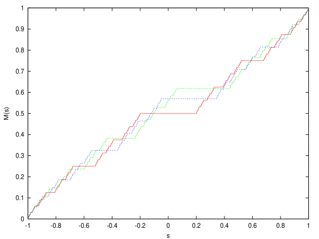
Fig. 10: Distribution functions $M(s):=\int_{-\infty}^{s}d\mu(s^{\prime})$ for three uniform Gibbs measures with the same $D_{q}(\mu)=D_{0}={\log 2}/({\log 5-\log 2})$, as described in the text.

To the contrary, linear iterated function systems [38, 39, 40, 41], in which we have at our disposal an unlimited number of maps of the kind (37), $l_{i}(s)=\delta_{i}s+\theta_{i}$, and associated probabilities $\pi_{i}$, $i=1,\ldots,M$ can approximate arbitrarily well any measure with bounded support [42]. These I.F.S. define invariant measures $\mu$ via the obvious generalization of eq. (32),

$$\int f(s)d\mu(s)=\sum_{i=1}^{M}\pi_{i}\int(f\circ l_{i})(s)d\mu(s).$$ (50)

Moreover, linearity of the maps implies the renormalization equation

$$p_{n}(\mu;l_{i}(s))=\sum_{k=0}^{n}\Gamma_{i,k}^{n}p_{k}(\mu;s).$$ (51)

The coefficients $\Gamma$ have a profound meaning, as they are the Lanczos vectors associated with a generalization of the Jacobi matrix ${\bf J}_{\mu}$ [43]. In ref. [8] I have employed eqs. (50),(51) in a similar fashion than in Sect. 11, to study the intermittency function $\beta(\alpha)$. It has not been possible, though, to close the asymptotic relations exactly, but only to obtain a sequence of approximation of the intermittency function. Nonetheless, this approximate renormalization theory has shown that the key to the asymptotic behavior of the moments $\nu_{\alpha}(t)$ lies in the properties of the coefficients $\Gamma$. Needless to say, these properties are rather elusive.

Fig. 11: Intermittency function $\beta(\alpha)$ for I.F.S. generated uniform Gibbs measures with the same spectrum of generalized dimensions, $D_{q}(\mu)=D_{0}={\log 2}/({\log 5-\log 2})$. Data plotted are for: two–maps I.F.S. (three lower coincident curves, crosses); a symmetrical three–maps I.F.S. (central curve, open squares), and an asymmetrical three–maps I.F.S. measure (top curve, filled squares).

In closing this paper I want to discuss an additional piece of evidence from [7] that might give us a clue on the general problem, and is still (to my knowledge) unexplained. Consider the set of linear I.F.S. generated by just two maps, for which

$$\pi_{i}=\delta_{i}^{D_{0}},\;\;i=1,2$$ (52)

where $D_{0}$ is a real number between zero and one, that must obviously satisfy the probability conservation equation

$$1=\sum_{i=1}^{2}\pi_{i}=\sum_{i=1}^{2}\delta_{i}^{D_{0}}.$$ (53)

Because of the latter equality, $D_{0}$ is the box-counting dimension of the support of $\mu$. Clearly, because of eqs. (52) and (53), only one parameter among the map weights and contraction rates is left free, and can be put in one to one relation with $D_{0}$.

Moreover, the two affine constants $\theta_{i}$ play no rôle in determining the power–law behavior of the moments $\nu_{\alpha}(t)$, since we can translate and stretch linearly the support of $\mu$ with the only effect of multiplying the F-B. functions by a complex number of modulus one, and of linearly rescaling their argument [44]. Notice finally that eq. (53) also implies that the I.F.S. is disconnected.

In conclusion, the family of two–maps linear IFS measures satisfying eq. (52) can be partitioned into equivalence classes labelled by the box–counting dimension $D_{0}(\mu)$. The distribution functions of three measures in the same equivalence class are displayed in Fig. 10. These measures enjoy distinctive properties. First of all, they are uniform Gibbs measures, according to the theory of Bowen [45]. Moreover, since eq. (20), with $\delta_{i}$ and $\pi_{i}$ in place of $l_{\sigma}$ and $\pi_{\sigma}$, and $H(x)=1$ instead of the asymptotic relation, defines the generalized dimensions of linear I.F.S. measures exactly, one finds easily that $D_{q}(\mu)=D_{0}(\mu)$ for all real values of $q$.

Now, figure 11 shows the functions $\beta(\alpha)$ extracted numerically for three I.F.S. belonging to the same equivalence class $D_{0}(\mu)=\frac{\log 2}{\log 5-\log 2}$. The coincidence of the curves (crosses) within numerical precision—that we have also verified for other values of $D_{0}$—lead us to conjecture that the intermittency function $\beta(\alpha)$ is an invariant of the equivalence classes defined above.

13 From linear I.F.S. to potential theory: another conjecture

Even prior to a formal proof of the conjecture just proposed, accepting its validity leads to interesting speculations, and raises intriguing questions. Clearly, the conjecture disproves any relation of the kind $\beta(\alpha)=D_{q(\alpha)}$, with $q$ a function of $\alpha$, like in the bounds (15), or in the Julia set relation (49). This is not necessarily bad news: it is just telling us once more that characteristics of the measure $\mu$ other than the generalized dimensions determine the dynamics: a few of these have been presented in this paper. How are the exponents $d(r)$ and $d(\omega)$ of eqs. (24) and (25) related, in and across the equivalence classes above? And the coefficients $\Gamma$ ? Moreover, we can also ask how curves with different values of $D_{0}$ map among themselves. But mostly, since eq. (52) is magnificent in its simplicity, is it there a simple argument to prove the conjecture?

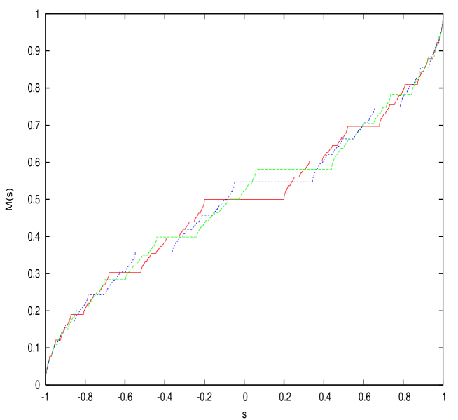
Fig. 12: Distribution functions $M(s):=\int_{-\infty}^{s}d\nu(s^{\prime})$ where $\nu$ are the equilibrium measures associated with the three I.F.S. measures of Fig. 10.

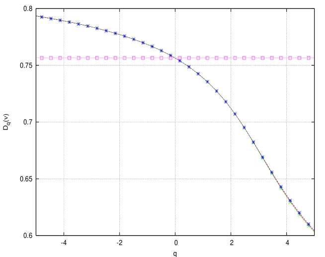
Fig. 13: Generalized dimensions of the three I.F.S. measures of Fig. 10 (squares, horizontal line) and of the associated equilibrium distributions (stars) of Fig. 12.

En suite, notice that the extension of the conjecture to I.F.S. with three or more maps, without further specifications, is not valid. In fact, an instructive counter–example is obtained setting $M=3$, and all contraction values and weights equal among themselves: $\delta_{i}=\delta<\frac{1}{3}$, $\pi_{i}=\frac{1}{3}$, for $i=1,2,3$. In this case, out of the three affine constants $\theta_{i}$, two can be set arbitrarily (for instance, so that $[-1,1]$ is the convex hull of the support of $\mu$), and one is left free to vary. This can be done so that the resulting I.F.S. is disconnected: its hierarchical structure is then composed of the iteration of three bands, the position of the central of which is variable. The one-parameter set of I.F.S. measures so obtained is composed of uniform Gibbs measures with $D_{q}(\mu)=D_{0}(\mu)=-\log(\delta)/\log(3)$. And yet, the functions $\beta(\alpha)$ are not invariant in this set: see figure 11, where $\delta$ is chosen so to obtain the same $D_{0}$ as in the two–maps case.

We can try an explanation of this fact. These latter three–maps I.F.S. measures have different quantum intermittency functions, even if they coincide “cylinderwise”, because their logarithmic potential equilibrium measures are different, since gaps between covering sets $I_{\sigma}$ have different geometric ratios, and consequently, we expect different asymptotic behavior of their orthogonal polynomials.

Having realized this, let us go back to the two–maps case. In what respect are then the equilibrium measures within the two–maps equivalence classes defined above “equivalent”? Direct inspection of their distribution functions, Fig. 10, provides no clue. It is Fig. 13 that contains the answer: the generalized dimensions of the equilibrium measures of two–maps I.F.S. in the same equivalence class are the same. One can therefore take the risk of putting forward a bolder conjecture: the intermittency function of uniform Gibbs measures, whose equilibrium measures are characterized by the same spectrum of generalized dimensions, are the same [46].

14 Conclusions

I have discussed in this paper a number of topics that have originally been developed by mathematical physicists interested in quantum mechanics, as it appears clearly from the list of references, but that would certainly profit a lot from the interest of specialists in orthogonal polynomials, special functions, and potential theory. In fact, my formulation via Fourier–Bessel functions, the original idea [47, 6] to study these problems in relation with Jacobi matrices of Iterated Function Systems, and my introduction of the renormalization approach of orthogonal polynomials denote clearly how much I owe to the community that has gathered for this conference, and that I had the fortune to meet back in my postdoc years here in Atlanta.

I have presented novel results on the asymptotic properties of F-B. functions for Julia set invariant measures, relating different asymptotics of the “wave–packets” $\nu_{\alpha}(N,\omega)$ to the properties of the invariant measure, and of its orthogonal polynomials. But mostly I have put forward open problems, numerical results, and conjectures that indicate–I hope–where to search for complete answers. How to turn this insight into a constructive technique for determining the intermittency function is the job that stays ahead. Having so arrived at the main topic of this conference, potential theory and its applications, I can certainly renew my best wishes to Ed, and retire in order.

Appendix: Numerical Techniques

In addition to standard procedures, the research described in this paper has required novel numerical algorithms for two main problems: the construction of Jacobi matrices of linear I.F.S., described in [43], [48], and the computation of the F-B. functions [11].

References

- [1] R.S. Strichartz, Fourier asymptotics of fractal measures, J. Funct. Anal. 89 (1990), pp. 154–187.
- [2] R.S. Strichartz, Self-similar measures and their Fourier transforms I, Indiana U. Math. J. 39 (1990), pp. 797–817.
- [3] R.S. Strichartz, Self-similar measures and their Fourier transforms II, Trans. Amer. Math. Soc. 336 (1993), pp. 335–361.
- [4] K.A. Makarov, Asymptotic Expansions for Fourier Transform of Singular Self-Affine Measures, J. Math. An. and App. 186 (1994), pp. 259–286.
- [5] K.S. Lau and J. Wang, Mean quadratic variations and Fourier asymptotic of self-similar measures, Monatsh. Math. 115 (1993), pp. 99–132.
- [6] I.Guarneri and G.Mantica, Multifractal Energy Spectra and their Dynamical Implications Phys. Rev. Lett. 73 (1994), pp. 3379–3382.
- [7] G. Mantica, Quantum Intermittency in Almost Periodic Systems Derived from their Spectral Properties, Physica D 103 (1997), pp. 576–589.
- [8] G. Mantica, Wave Propagation in Almost-Periodic Structures, Physica D 109 (1997), pp. 113–127.
- [9] G. Mantica and S. Vaienti, The Asymptotic Behaviour of the Fourier Transforms of Orthogonal Polynomials I: Mellin Transform Techniques, preprint mp–arc 04–314 (2004), submitted to Annales Henri Poincaré.
- [10] G. Mantica and D. Guzzetti, The Asymptotic Behaviour of the Fourier Transforms of Orthogonal Polynomials II: IFS measures and Quantum Mechanics, preprint mp–arc 04–361 (2004), submitted to Annales Henri Poincaré.
- [11] G. Mantica Fourier Transforms of Orthogonal Polynomials of Singular Continuous Spectral Measures, in Int. Ser. Numer. Mathematics, 131 (1999), pp. 153–163, W. Gautschi and G. Opfer Eds.
- [12] For , is the normalization condition (7). For negative values of we can still define moments by letting the summation in eq. (8) start from . These moments are of interest when completing the analogy with theory of the generalized dimension of singular measures.
- [13] I.Guarneri, H. Schulz Baldes, Lower Bounds on Wave-Packet Propagation by Packing Dimensions of Spectral Measures, Math. Phys. Elec. J. 5 (1999), pap. 1.
- [14] J.M. Barbaroux, J.M. Combes, and R. Montcho, Remarks on the relation between quantum dynamics and fractal spectra, J. Math. Anal. Appl. 213 (1997), pp. 698–772.
- [15] I.Guarneri, H. Schulz Baldes, Intermittent Lower Bound on Quantum Diffusion, Lett. Math. Phys. 49 (1999), pp. 317–324.
- [16] J.M. Barbaroux, F. Germinet, S. Tcheremchantsev, Fractal dimensions and the phenomenon of intermittency in quantum dynamics, Duke Math. J. 110 (2001), pp. 161–193.
- [17] S. Tcheremchantsev, Mixed lower bounds for quantum transport, J. Funct. Anal. 107 (2003), pp. 247–282.
- [18] R. Ketzmerick, K. Kruse, S. Kraut and T. Geisel, What Determines the Spreading of a Wave Packet?, Phys. Rev. Lett. 79 (1997), pp. 1959–1963.
- [19] In ref. [18], the quantity is improperly called the correlation dimension of the eigenfunctions, a name that in the physical literature denotes a different quantity, whose value is not universal, as it depends on the eigenfunction under investigation. It must also be remarked that the authors of [18] deal with proper eigenfunctions, since they consider finite truncations of the Jacobi Hamiltonian , that obviously have pure point spectrum. The theory of Gaussian integration shows that this is an approximation of our general formalism.
- [20] Y. Pesin, Dimension theory in dynamical system: contemporary views and applications, Univ. Chicago Press, (1996).
- [21] J.M. Barbaroux, F. Germinet, S. Tcheremchantsev, Generalized fractal dimensions: equivalence and basic properties, J. Math. Pures Appl. 80 (2001), pp. 977–1012.
- [22] R. Ketzmerick, G. Petschel, and T. Geisel, Slow decay of temporal correlations in quantum systems with Cantor spectra, Phys. Rev. Lett. 69 (1992), pp. 695–698.
- [23] J.M. Barbaroux, F. Germinet, S. Tcheremchantsev, Transfer matrices and transport for 1D Schrödinger operators with singular spectrum, Ann. Inst. Fourier 54 (2004), pp. 787–830.
- [24] R. Killip, A. Kiselev, and Y. Last, Dynamical upper bounds on wavepaket spreading, Amer. J. Math. 125 (2003), pp. 1165–1198.
- [25] I. Guarneri, H. Schulz Baldes, Upper bounds for quantum dynamics governed by Jacobi matrices with self–similar spectra, Rev. Math. Phys. 11, (1999) pp. 1249–1268.
- [26] J.-M. Barbaroux, H. Schulz Baldes, Anomalous transport in presence of singular continuous spectral measures, Ann. Inst. H. Poincaré Phys. Théo. 71 (1999) pp. 539-559.
- [27] J.M. Combes, and G. Mantica, Fractal dimensions and quantum evolution associated with sparse potential Jacobi matrices, in Long time behavior of classical and quantum systems, Ser. Concr. Appl. Math. 1, World Sci. Publishing, River Edge, NJ, 2001, pp. 107–123.
- [28] S. Jitomarskaya, Y. Last, Dimensional Hausdorff Properties of Singular Continuous Spectra, Phys. Rev. Lett. 76 (1996) 1765-1769.
- [29] A. Kiselev and Y. Last, Solutions, spectrum, and dynamics for Schrödinger operators on infinite domains, Duke Math. J. 102 (2000), pp. 125–150.
- [30] L. Brillouin, Wave Propagation in Periodic Structures, Dover Publications, NY, (1953).
- [31] M.F. Barnsley, J.S. Geronimo, and A.N. Harrington, Infinite-Dimensional Jacobi Matrices Associated With Julia Sets, Proc. Am. Math. Soc. 88 (1983), pp. 625–630.
- [32] J. Bellissard, D. Bessis, and P. Moussa, Chaotic States of Almost Periodic Schrödinger Operators, Phys. Rev. Lett. 49 (1982), pp. 702–704.
- [33] Pitcher and Kinney, Some connections between ergodic theory and the iteration of polynomials, Ark Mat. 8 (1969) pp. 25–32.
- [34] G. Mantica, Quantum Intermittency: Old or New Phenomenon? J. Phys. IV France 8 (1998), pp. Pr6-253–262.
- [35] In ref. [18], various examples are exhibited for which the bound is significantly better than . Yet, the (incorrect) statement is made that is an upper bound to for all negative values of (see [12]). Where this to be true, it would imply that , where the latter quantity can be defined by a limiting procedure, when is continuous. To the contrary, in Sect. 11 we show a case where .
- [36] F. Piéchon Anomalous diffusion properties of wave packets on quasiperiodic chains, Phys. Rev. Lett. 76 (1996), pp. 4372–4375.
- [37] J. Bellissard, I. Guarneri, H. Schulz-Baldes, Phase–averaged transport for quasi–periodic Hamiltonians, Comm. Math. Phys. 227 (2002) pp. 515–539.
- [38] J. Hutchinson, Fractals and Self-Similarity, Indiana J. Math. 30 (1981), pp. 713–747.
- [39] M.F. Barnsley and S.G. Demko, Iterated Function Systems and the Global Construction of Fractals, Proc. R. Soc. London A 399 (1985), pp. 243–275.
- [40] M.F. Barnsley, Fractals Everywhere, Academic Press, New York, (1988).
- [41] The asymptotics of the moments of I.F.S. measures has been studied in W. Goh and J. Wimp, Asymptotics for the moments of singular distributions, J. Approx. Theory 74 (1993) pp. 301–334; A generalized Cantor-Riesz-Nagy function and the growth of its moments, Asymptotic Anal. 8 (1994) pp. 379–392.
- [42] C.R. Handy and G. Mantica, Inverse Problems in Fractal Construction: Moment Method Solution, Physica D 43 (1990), pp. 17–36.
- [43] G. Mantica, A Stieltjes Technique for Computing Jacobi Matrices Associated With Singular Measures, Constr. Appr. 12 (1996), pp. 509–530.
- [44] Of course, with the exception of the case where the two I.F.S. maps have the same common fixed point, that so becomes the degenerate support of .
- [45] R. Bowen, Equilibrium States and the Ergodic theory of Anosov Diffeomorphisms, Lect. Notes in Math. 470, Springer-Verlag Berlin (1975).
- [46] Notice that Gibbs uniformity is required in this conjecture. In fact, it is not enough to require that measures be characterised by equilibrium measures with the same generalized dimensions. In fact, choose any of the two–maps I.F.S. of this section, and change the weights while keeping the contraction rates fixed. Since the equilibrium measure depends only on the support of , it does not change in the process. To the contrary, as shown already in [6], in these circumstances the intermittency functions are sensitive to the weights.
- [47] D. Bessis and G. Mantica, Orthogonal Polynomials associated to Almost Periodic Schrödinger Operators, J. Comp. Appl. Math., 48 (1993), pp. 17–32.
- [48] G. Mantica On Computing Jacobi Matrices associated with Recurrent and Möbius Iterated Functions Systems, J. Comp. Appl. Math. 115 (2000), pp. 419–431.