2D growth processes:
SLE and Loewner chains

Abstract

This review provides an introduction to two dimensional growth processes. Although it covers a variety processes such as diffusion limited aggregation, it is mostly devoted to a detailed presentation of stochastic Schramm-Loewner evolutions (SLE) which are Markov processes describing interfaces in 2D critical systems. It starts with an informal discussion, using numerical simulations, of various examples of 2D growth processes and their connections with statistical mechanics. SLE is then introduced and Schramm’s argument mapping conformally invariant interfaces to SLE is explained. A substantial part of the review is devoted to reveal the deep connections between statistical mechanics and processes, and more specifically to the present context, between 2D critical systems and SLE. Some of the SLE remarkable properties are explained, as well as the tools for computing with SLE. This review has been written with the aim of filling the gap between the mathematical and the physical literatures on the subject.

and

Notations:
${\bf P}[\cdots]=$ probability,
${\bf E}[\cdots]=$ expectation.
${\bf P}[\cdots|C]=$ probability conditioned on $C$,
${\bf E}[\cdots|C]=$ expectation conditioned on $C$.
$\mathcal{F}_{t}=$ filtration by $\sigma$-algebras.
$B_{t}=$ normalized Brownian motion with ${\bf E}[B_{t}B_{s}]={\rm min}(t,s)$.
$\xi_{t}=\sqrt{\kappa}\,B_{t}$, with covariance ${\bf E}[\xi_{t}\xi_{s}]=\kappa\ {\rm min}(t,s)$.
$\mathbb{U},\ \mathbb{D}=$ (planar) domain, ie. connected and simply connected open subset of the complex plane $\mathbb{C}$.
$\mathbb{K}=$ hulls, ie. connected compact subset of a domain $\mathbb{D}$ such that $\mathbb{D}\setminus\mathbb{K}$ is a domain.
$g_{\mathbb{K}}=$ holomorphic map uniformizing $\mathbb{D}\setminus\mathbb{K}$ into $\mathbb{D}$,
$f_{\mathbb{K}}:\mathbb{D}\to\mathbb{D}\setminus\mathbb{K}$ its inverse.
$\gamma_{[0,t]}=$ the SLE curve with tip $\gamma_{t}$ at time $t$.
$\mathbb{K}_{t}=$ the SLE hull at time $t$.
$\mathbb{D}_{t}\equiv\mathbb{D}\setminus\mathbb{K}_{t}$, the domain $\mathbb{D}$ with the hull $\mathbb{K}_{t}$ removed.
$g_{t}:\mathbb{D}_{t}\to\mathbb{D}$, the SLE Loewner map and $f_{t}:\mathbb{D}\to\mathbb{D}_{t}$, its inverse.
$U_{t}=g_{t}(\gamma_{t})$= image of the tip of the SLE curve.
$h_{t}:\mathbb{D}_{t}\to\mathbb{D}$, mapping the tip of the curve back to its starting point.
$\mathfrak{vir}=$ the Virasoro algebra.
$\mathfrak{g}_{h}$= a group element associated to a map $h$.
$G_{h}=$ representation of $\mathfrak{g}_{h}$ in CFT Hilbert spaces.
$h_{r;s}=[(r\kappa-4s)^{2}-(\kappa-4)^{2}]/16\kappa$ for $c=1-6(\kappa-4)^{2}/4\kappa$.
$|\psi_{r;s}\rangle=$ highest weight vector with dimension $h_{r;s}$.
$\varphi_{\delta}(x)=$ boundary primary field with dimension $\delta$.
$\psi_{r;s}(x)=$ degenerate boundary primary field with dimension $h_{r;s}$.
$\Phi(z,\bar{z})=$ bulk primary fields.
$\Phi_{r;s}(z,\bar{z})=$ degenerate bulk primary field with dimension $2h_{r;s}$.
$\langle\cdots\rangle_{\mathbb{D}}=$ CFT correlation functions in a domain $\mathbb{D}$.
$Z_{\mathbb{D}}=$ statistical partition function in a domain $\mathbb{D}$.
$\prec\cdots\succ_{\mathbb{D}}=$ statistical average in a domain $\mathbb{D}$.

1 Introduction

The main subject of this report is stochastic Loewner evolutions, and its interplay with statistical mechanics and conformal field theory.

Stochastic Loewner evolutions are growth processes, and as such they fall in the more general category of growth phenomena. These are ubiquitous in the physical world at many scales, from crystals to plants to dunes and larger. They can be studied in many frameworks, deterministic of probabilistic, in discrete or continuous space and time. Understanding growth is usually a very difficult task. This is true even in two dimensions, the case we concentrate on in these notes. Yet two dimensions is a highly favorable situation because it allows to make use of the power of complex analysis in one variable. In many interesting cases, the growing object in two dimensions can be seen as a domain, i.e. a contractile open subset of the Riemann sphere (the complex plane with a point at infinity added) leading to a description by so-called Loewner chains.

Stochastic Loewner evolution is a simple but particularly interesting example of growth process for which the growth is local and continuous so that the resulting set is a curve without branching. Of course other examples have been studied in connection with 2d physical systems. The motivations are sometimes very practical. For instance, is it efficient to put a pump in the center of oil film at the surface of the ocean to fight against pollution? The answer has to do with the Laplacian growth or Hele-Shaw problem. The names diffusion limited aggregation and dielectric breakdown speak for themselves. Various models have been invented, sometimes with less physical motivation, but in order to find more manageable growth processes. These include various models of iterated conformal maps, etc. As mentioned above, in most cases the shape of the growing domains is encoded in a uniformizing conformal map whose evolution describes the evolution of the domain. The dynamics can be either discrete or continuous in time, it can be either deterministic or stochastic. But the growth process is always described by a Loewner chain.

So we shall also give a pedagogical introduction to the beautiful subject of general Loewner chains. We wanted to show that it leads to many basic mathematical structures whose appearance in the growth context is not so easy to foresee, like integrable systems and anomalies to mention just a few. We have also tried to stress that some growth processes have rules which are easy to simulate on the computer. A few minutes of CPU are enough to get an idea of the shape of the growing patterns, to be convinced that something interesting and non trivial is going on, and even sometimes to get an idea of fractal dimensions. This is of course not to be compared with serious large scale simulations, but it is a good illustration of the big contrast between simple rules, complex patterns and involved mathematical structures. However, other growth models, and among those some have been conjectured to be equivalent to simple ones, have resisted until recently to precise numerical calculations due to instabilities.

To avoid any confusion, let us stress that being able to describe a growth process using tools from complex analysis and conformal geometry does not mean that the growth process itself is conformally invariant at all. Conformal invariance of the growth process itself puts rather drastic conditions on the density that appears in the Loewner chain and lead to stochastic Loewner evolutions.

Why do we think the emergence of stochastic Loewner evolutions is so important ? This question has several answers at various levels.

A first obvious answer is that stochastic Loewner evolutions are among the very few growth processes that can be studied analytically in great detail. The other growth processes we shall present in these notes are still very poorly understood, and many basic qualitative question like universality classes are still debated.

A second obvious answer is that stochastic Loewner evolutions solve a problem that had remained open for two decades despite the fact that the importance of conformal invariance had been fully recognized : the description of conformally invariant extended objects. This obvious answer is in fact best incorporated into a deeper one which is rooted in history.

There is a natural flow in the life of scientific discoveries, and conformal field theory was no exception to the rule.

Starting in 1984, conformal field theory has been an object of study for itself during a decade or so, revealing a fascinating richness. At a critical point and for short range interactions, statistical mechanics systems are expected to be conformally invariant. The argument for that was given two decades ago in the seminal paper on conformal field theory [21]. The rough idea is the following. At a critical point, a system becomes scale invariant. If the interactions on the lattice are short range, the model is described in the continuum limit by a local field theory and scale invariance implies that the stress tensor is traceless. In two dimensions this is enough to ensure that the theory transforms simply –no dynamics is involved, only pure kinematics– when the domain where it is defined is changed by a conformal transformation. The local fields are classified by representations of the infinite dimensional Virasoro algebra and this dictates the way correlation functions transform. This has led to a tremendous accumulation of exact results.

From the start, conformal field theory was also seriously directed towards applications, and this is even more true now that it has reached technical maturity. During the last twenty years or so, conformal field theory has become a standard tool, and a very powerful one indeed, to tackle a variety of problems. Significant progresses in condensed matter theory owe a lot to conformal field theory : computation of universal amplitudes for the Kondo problem, various aspects of the (fractional) quantum Hall effect, Luttinger liquid theory are just a few examples. String theory has sowed conformal field theory but also collected a lot.

This shift from goal to tool does not mean that everything is understood. In fact nothing could be less exact. A situation that is well under control is that of Virasoro unitary minimal models. The Hilbert space of the system splits as a finite sum of representations of the Virasoro algebra, each associated to a (local) primary field, and the corresponding correlation functions can be described rather explicitly. However, the initial hope of classifying all critical phenomena in two dimensions has vanished. Work has concentrated on special, manageable, classes of theories generalizing the Virasoro unitary minimal models. The most user-friendly theories are minimal for algebras extending the Virasoro algebra. For these a finite number of representations suffices to describe many physical properties of the underlying model. Even the classification of minimal theories is a formidable task and it is far from obvious that the goal will be achieved ever. Surprisingly maybe, adding unitarity on top of minimality does not help much.

On the other hand, many (most of the ?) important applications of conformal field theories, emerging for instance from string theory or disordered systems, involve non unitary and non minimal models. The presence of an infinite number of fields/representations makes their study extremely complex, and no unifying principle has emerged so far. Great ingeniosity has been devoted obtaining a core of deep and interesting but partial, scattered and sometimes controversial results.

Concerning interfaces –for instance domain boundaries– of critical systems in two dimensions, the situation was until recently also quite unsatisfactory. The few significant results obtained using conformal field theory before the emergence of stochastic Loewner evolutions were the outcome of highly clever craftsmanship and had nothing to do with systematic techniques. It should be stressed however that formulæ like Cardy’s percolation probability distribution had not escaped the notice of mathematicians, and have been a source of motivation for them that has finally lead to Schramm’s breakthrough.

Analysis of the interplay between conformal field theory and stochastic Loewner evolutions leads to a very exciting and positive message. The conformal field theories needed to understand interfaces have many nasty features, non minimality, non unitarity, etc. However for the first time physicists have a rigorous mathematical parapet, they can check their predictions and learn how to tame the pathologies that have prevented systematic progress until now. We are a long way from such an horizon, but in the long run this might be the main impact of stochastic Loewner evolutions in physics.

The Swiss army knife of axiomatic and/or constructive quantum field theory contains in particular algebra and representation theory, complex variables (for the analyticity of correlation functions and the S matrix in axiomatic field theory) and measure theory (in constructive quantum field theory). It is a happy accident, without deep significance, that these tools are also at the heart of the understanding of two dimensional critical interfaces that has emerged at the turn of the millenium.

Non local objects like interfaces are not classified by representations of the Virasoro algebra but the reasoning that led O. Schramm to the crucial breakthrough [118], i.e. the definition of stochastic Loewner evolutions, rests on a fairly obvious but cleverly exploited statement of what conformal invariance means for an interface. Surprisingly it allows to turn this problem into growth problem of Markovian character. From a naïve viewpoint, this is one of the most surprising features of stochastic Loewner evolutions. Maybe this is one of the reasons why they were not discovered by the impressive army of conformal field theorists. After all, in a statistical mechanics system with appropriate boundary conditions, a complete domain boundary is present in each sample, any dynamics building it piece after piece seems rather artificial, and correlations between the pieces at not short range. The discrete geometric random curves on which the interest of mathematicians has focused also do not give a clue. While percolation and some of its cousins and descendants can be very naturally viewed as growth processes, this is more the exception than the rule. The case of self avoiding walks is a significant example. The literature on the subject repeatedly stresses that changing the length of a self avoiding walk by one changes the measure globally in a complicated.

For some years, probabilistic techniques have been applied to interfaces, leading to a systematic understanding that was lacking on the conformal field theory side. There is now a satisfactory understanding of interfaces in the continuum limit. However, from a mathematical viewpoint, giving proofs that a discrete interface on the lattice has a conformally invariant limit remains a hard challenge and only a handful of cases has been settled up to now.

The organization of these notes is as follows.

Section 2 is an informal presentation of discrete lattice models, first of geometric random curves – starting with the most growth process like, percolation, and ending with the self avoiding walk–, then of statistical mechanics domain boundaries –the Ising model, the $O(n)$ models and $Q$-state Potts model–, ending with a few growth processes that are not expected to be conformally invariant in the continuum limit, like diffusion limited aggregation.

The first goal is to get some familiarity with the basic objects that are studied in the rest of this report. In particular we show that geometric random curves are easy to simulate and produce beautiful and complicated patterns. We emphasize that many variants of these geometric random curves are still to be discovered and studied. We also recall that appropriate statistical mechanics models domain boundaries are described by geometric random curves.

Section 3 introduces Loewner chains which are one of the basic tools to describe growth process in two dimensions. Riemann’s mapping theorem states that two domains (= connected and simply connected open sets different from $\mathbb{C}$ itself) are conformally equivalent. This allows to use a fixed simple reference domain, which is usually taken as the upper-half plane or the in/out side of the unit disk. This conformal equivalence is unique once an appropriate normalization, which may depend on the growth problem at hand, has been chosen. Cauchy’s theorem allows to write down an integral representation for the conformal map as an integral along the boundary of the reference domain, involving a (positive because of growth) density which is time dependent. A nice way to specify the growth rule is often directly on this density. The time derivative of the conformal map has an analogous representation, leading to an equation called a Loewner chain. Local growth is when the density is a finite sum of Dirac peaks. The positions of these peaks are functions of time and serve as of the Loewner evolution. This case is the most important for the ensuing study.

Schramm-Loewner evolutions (also called stochastic Loewner evolutions), the object of section 4 occur when the Loewner evolution measure is a single delta peak and the associated parameter is a Brownian motion. We reproduce Schramm’s argument that this is exactly the setting that describes conformally invariant measures on random curves. SLE has a number of avatars, depending on whether the random curves go from one boundary point to another to another boundary point –chordal SLE–, to a point in the bulk –radial SLE– or to an interval on the boundary –dipolar SLE–. The diffusion coefficient, i.e. the normalization of the Brownian motion $\kappa$ is the only parameter, and qualitative and quantitative features of SLE_κ samples depend on it. SLE_κ can be generalized to SLE_κ,ρ which we review briefly. The group theoretic formulation of the various SLEs as a random processes on groups is also presented

Section 5 makes contact with statistical mechanics and the interplay between the measure on domain boundaries and the full initial measure on configuration. Roughly speaking, to check that a measure on random curves is inherited from a statistical mechanics model, one has to check that a correlation function with fixed domain boundary, when averaged over the random curve measure supposed to describe the domain boundary, yields back the original correlation function. We rephrase this statement in terms of martingales. These observations, which are in general of little use –not only because nobody has a measure on domains boundaries to offer but also because the computation of correlation functions with fixed domain boundaries is well out of reach– becomes very efficient when conformal invariance is imposed. Indeed conformal field theory is able to reduce kinematically correlation functions in any domain to correlation function in a reference domain, and the measure on domain boundaries is an SLE. Hence Itô calculus becomes an efficient tool. This strategy is made explicit in the operator formalism for the variants of SLE introduced before. Its predictive power is illustrated on how it leads naturally to multiple SLEs.

Section 6 is concerned with geometric structures and properties of SLE samples. The locality property of SLE₆ (related to percolation) and the restriction property of SLE_8/3 (related to self avoiding walks) are presented. The application to the fractal dimension of the exterior perimeter of Brownian excursion is explained. Duplantier’s predictions concerning the fractal spectrum of harmonic measures of conformally invariant hulls are also presented. The section ends with a friendly introduction to the Brownian loop soup.

Section 7 illustrates how to compute explicit significant properties of SLE using tools from stochastic calculus and/or conformal field theories. Boundary hitting probabilities, crossing formulæ  fractal dimensions, etc are computed. The last part is devoted to a list of references to other important results.

Section 8 is an introduction to the study of more general growth processes via discrete and continuous time Loewner chains. The relationship between Laplacian growth and integrability is presented.

For the sake of completeness, we have included two appendices. While appendix B on conformal field theory basics is rather short, appendix A is a more substantial –but of course very limited– introduction to probabilistic methods and stochastic processes. This appendix contains enough material to help understand the probabilistic tools used systematically in the rest of the report: martingales, Brownian motion, Itô calculus. It seemed to us that these subject are not so familiar to physicists and that systematic reference to the probabilistic literature (excellent as it can be) would be awkward. This has not prevented us from giving a list of books that have proved valuable for us.

2 Constructive examples

Before we embark on more formal aspects, it is good to give a few explicit examples of the kind of structures that we aim to study, i.e. conformally invariant random curves in two dimensions.

SLE gives a description of such objects directly in the continuum, but the starting point is usually a discrete model of random curves on a lattice. It is a tough job, only achieved for a handful of cases at the time of this writing, to start from such a definition and show that in the continuum limit one recovers a conformally invariant probability distribution. The variety of examples will amply show that a general heuristic criterion to decide whether or not a given discrete interface distribution has a conformally invariant continuum limit is not so easy to exhibit. In quantum field theory, it is not easy to exhibit local field theories which are scale invariant but not conformally invariant [35], and there is a heuristic argument based on locality to explain why it is so. But a similar heuristic argument for SLE does not exist. We shall make a few remarks on this in the sequel.

Another feature of SLE is to present the random curves as growth processes: SLE gives a recipe to accumulate (infinitesimal) pieces on top of each other, with a form of Markov property to be elucidated below. For discrete models, a natural growth process definition is more the exception than the rule.

Let us also note that the favorite examples in the mathematics and physics community are not the same. Physicists are used to start from lattice models where each lattice site carries a degree of freedom, and the random distribution of these degrees of freedom is derived from a Boltzmann weight, i.e. an unnormalized probability distribution. In the presence of appropriate boundary conditions, some one dimensional defects appear. The weight of a defect of given shape can (in principle) be obtained by summing the Boltzmann weights over all configurations exhibiting this defect. On the other hand, mathematicians have often concentrated on interfaces with a more algorithmic and direct definition. For the cost of numerical simulations, this makes a real difference. At a more fundamental level however, the distinction is artificial because it is usually possible to cook up Boltzmann weights (for local degrees of freedom and with local interactions) that do the job of reproducing an interface distribution defined by more direct means or at least an interface distribution which is in the same universality class.

The model whose definition fits best with the image of a growth process is percolation, and we shall start with it. The growth aspect of the two next examples, the harmonic navigator (the GPL version of Schramm’s harmonic explorer) and loop-erased random walks, is only slightly less apparent. But self avoiding random walks to be introduced right after are of a quite different nature. We shall illustrate these cases with baby numerical simulations, referring the interested readers to the specialized literature for careful and clever large scale studies [140] and [76, 77, 78]. Our aim is mainly to give some concrete pictures of these remarkably beautiful objects. We shall also see on concrete examples that the landscape of algorithms used to produce the curves is rather varied and largely unexplored, sheltering fundamental problems.

We shall then consider interfaces defined via lattice models in the cases of the Potts and $O(n)$ models, with some pictures for the Ising model.

We shall finally define diffusion limited aggregation (DLA), a growth process which is expected to have a scaling but no conformally invariant continuum limit. DLA, together with its cousins and descendants, will reappear at the end of these notes because many of those can be defined via Loewner chains.

We start with some basic definitions.

In the sequel we shall often need the notion of a lattice domain.

A square lattice domain $\mathbb{D}$ is a domain in the usual sense, which can be decomposed as a disjoint union of open squares with side length 1 (faces), open segments of length 1 (edges) and points (vertices), in such a way that each open segment belongs to the boundary of two open squares and each vertex belongs to the boundary of four open segments. Unless stated explicitly, we assume that the number of faces is finite.

An admissible boundary condition is a couple of distinct points $(a,b)$, $a,b\notin\mathbb{D}$ such that there is a path from $a$ to $b$ in $\mathbb{D}$ i.e. a number $n\geq 1$ and a sequence $s_{1},\cdots,s_{2n+1}$ where $a=s_{1},b=s_{2n+1}$, the $s_{2m+1}$, $1\leq m<n$, (if any) are distinct vertices of the decomposition of $\mathbb{D}$ and the $s_{2m}$, $1\leq m<n$, are distinct edges of the decomposition of $\mathbb{D}$ with boundary $\{s_{2m-1},s_{2m+1}\}$. Any such path splits $\mathbb{D}$ into a left and a right piece.

If $s_{1},\cdots,s_{2n+1}$ is a path from $a$ to $b$ in $\mathbb{D}$ and $0\leq m<n$, the set $\mathbb{D}^{\prime}$ obtained by removing from $\mathbb{D}$ the sets $s_{l}$, $1<l\leq s_{2m+1}$ is still a domain, and $(s_{2m+1},b)$ is an admissible boundary condition for $\mathbb{D}^{\prime}$.

Similar definitions and properties would hold for an hexagonal lattice domain, regular hexagons with (say) side of length 1 replacing the squares, and three replacing four. The two examples in fig.1 will probably make obvious what kind of domain we have in mind.

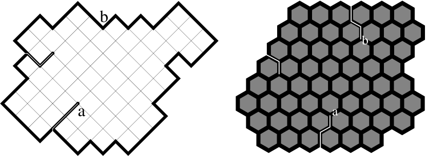
Figure 1: Example of square and hexagonal lattice domains.

Our main interest in the next subsections will be in measures on paths from $a$ to $b$ in $\mathbb{D}$ when $\mathbb{D}$ is a lattice domain and $(a,b)$ an admissible boundary condition.

Hexagonal lattice domains have useful special properties. Suppose $(\mathbb{D},a,b)$ is an hexagonal lattice domain with admissible boundary condition. The right (resp. left) hexagons are by definition those which are on the right (resp. left) of every path from $a$ to $b$ in $\mathbb{D}$. Left and right hexagons are called boundary hexagons. The other hexagons of $\mathbb{D}$ are called inner hexagons. Color the left hexagons in black (say) and the right hexagons in white as in Fig.2 on the left. If one colors the inner hexagons arbitrarily in black or white, then there is a single path from $a$ to $b$ in $\mathbb{D}$ such that the hexagon on the left (resp. right) of any of its edges is black (resp. white). This is illustrated in fig.2 on the right. This path can be defined recursively because $a$ is on the boundary of at least one left and at least one right hexagon: as $a$ is not in $\mathbb{D}$, in any coloring there is exactly one edge in $\mathbb{D}$ with $a$ on its boundary and bounding two hexagons of different colors. Start the path with this edge and go on.

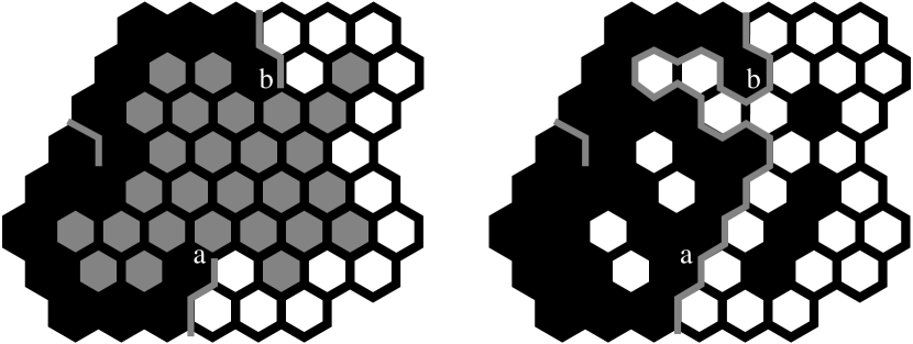
Figure 2: Left : the boundary of an hexagonal lattice domain with boundary conditions. Right : the interface associated to a configuration.

All the examples of interfaces we shall deal with in the sequel can be defined on arbitrary hexagonal lattice domain with admissible boundary condition, though sometimes we shall use square lattice domains. Geometrical examples will define directly a law for the interface or a probabilistic algorithm to construct samples. Examples from statistical mechanics will give a weight for each coloring of the inner hexagons, and the law for the interface will be derived (at least in principle) from this more fundamental weight. The model of interface can depend on some parameters, called collectively $p$ (for instance, temperature can be one of those).

Because arbitrary domains can be used, the statement of conformal invariance is non trivial and can be checked numerically. Fix an interface model and take a sequence of lattice domains $(\mathbb{D}_{n},a_{n},b_{n})$ and of positive scales $s_{n}\rightarrow 0^{+}$ such that (in an obvious notation) $s_{n}(\mathbb{D}_{n},a_{n},b_{n})$ converges to a domain with two boundary points marked, $(\mathbb{D},a,b)$. A continuum limit exists when there is a (domain independent) function $p(s)$ such that the distribution of interfaces in $s_{n}(\mathbb{D}_{n},a_{n},b_{n})$ with parameters $p(s_{n})$ converges to some limit. Then, different domains can be compared and conformal invariance can be checked on good lattice approximations of these domains.

2.1 Geometrical examples

2.1.1 Percolation

Let $(\mathbb{D},a,b)$ be an hexagonal lattice domain with admissible boundary condition. Color the left hexagons in black (say) and the right hexagons in white. A configuration is a choice of color (black or white) for the inner hexagons. Give each configuration the same probability. Equivalently, the colors of the inner hexagons are independent random variables taking each color with probability $1/2$. We could also introduce some asymmetry between the colors, but our main interest will be in the symmetric case, because it has a continuum limit, without adjusting any parameters.

As recalled above, each configuration defines an interface, i.e. the unique path from $a$ to $b$ in $\mathbb{D}$ such that the hexagon on the left (resp. right) of any of its edges is black (resp. white), see fig.3. Hence the probability distribution on configurations induces a probability distribution on paths from $a$ to $b$ in $\mathbb{D}$. This is called the (symmetric) percolation probability distribution.

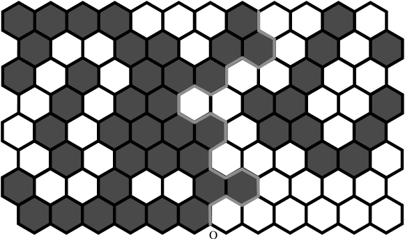
Figure 3: The definition of the percolation interface.

Because inner hexagon colors are independent, it is easy to compute the probability of a percolation path from $a$ to $b$ in $\mathbb{D}$ : if a path has an edge in common with $l$ distinct inner faces of $\mathbb{D}$, its probability is $2^{-l}$. The weight is given by a purely local rule. If $(\mathbb{D}^{\prime},a,b)$ is another hexagonal lattice domain with admissible boundary condition, a path common to $(\mathbb{D},a,b)$ and $(\mathbb{D}^{\prime},a,b)$ touching the same boundary and inner hexagons in both domains has the same probability in both domains : the percolation interface does not depend on the distribution of black and white sites away from itself. This is called locality, a property that singles out percolation.

In particular, locality allows to view percolation as a simple growth process, defined as follows. If $a$ is incident to no inner hexagon of $\mathbb{D}$, there is no choice in the first step of a path from $a$ to $b$ in $\mathbb{D}$. Else, $a$ is incident to exactly one inner hexagon of $\mathbb{D}$. Color it black or white using a fair coin, and make a step along the edge of $\mathbb{D}$ adjacent at $a$ whose adjacent faces have different colors. Then remove from $\mathbb{D}$ the edge corresponding to the first step and its other end point, call it $\dot{a}$ to get a new domain $\dot{\mathbb{D}}$. If $\dot{a}=b$ stop. Else $(\dot{\mathbb{D}},\dot{a},b)$ is a new hexagonal domain with admissible boundary condition and one can iterate as shown on the fig.4.

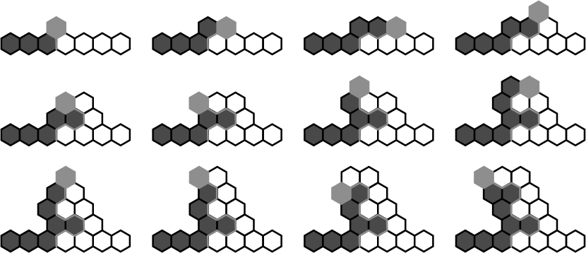
Figure 4: The percolation interface as a growth process.

There is exactly one coin toss for each inner face of $\mathbb{D}$ touching an edge of the path : this toss takes place the first time the inner face is touched by the tip of the path. In the rest of the process, this face becomes a boundary hexagon. Hence this growth process gives the percolation measure.

A geometry which is of frequent use is to pave the upper-half plane with regular hexagons and impose that the left (resp. right) hexagon be those intersecting the negative (resp. positive) real axis. This is an example with an infinite number of faces. No limiting procedure (taking larger and larger finite approximations of the upper-half plane) is necessary to get the correct weight for the initial steps of the percolation interfaces, again because of locality.

Fig.5 shows a few samples. They join the middle horizontal sides of similar rectangles of increasing size. The pseudo random sequence is the same for the four samples.

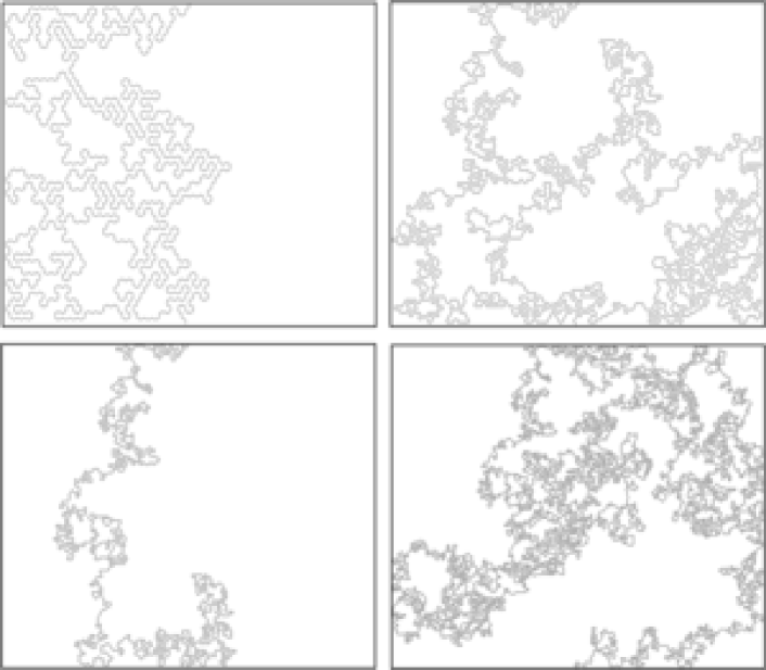
Figure 5: Samples of the percolation interface for increasing sizes.

Even for small samples, the percolation interface makes many twists and turns. By construction, the percolation interface is a simple curve, but with the resolution of the figure, the percolation interface for large samples does not look like a simple curve at all!

To estimate the (Hausdorff, fractal) dimension of the percolation interface, we have generated samples in similar rectangular domains of different sizes and made the statistics of the number of steps $S$ of the interface as a function of the size $L$ of the rectangle domain. One observes that $S\propto L^{\delta}$ and a modest numerical effort (a few hours of CPU) leads to $\delta=1.75\pm.01$.

The percolation interface is build by applying local rules involving only a few nearby sites, and we could wave our hands to argue that its scale invariance should imply its conformal invariance in the continuum limit. But the percolation process is one among the few systems that has been rigorously proved to have a conformally invariant distribution in the continuum limit, the fractal dimension being exactly $7/4$. As suggested by numerical simulations, the continuum limit does not describe simple curves but curves with a dense set of double points, and in fact the –to be defined later– SLE₆ process describes not only the percolation interface but also the percolation hull, which is the complement of the set of points that can be joined to infinity by a continuous path that does not intersect the percolation interface. As we shall see later, among SLE_κ’s, SLE₆ is the only one that satisfies locality, so what is really to prove in this case is conformal invariance in the continuum limit (a nontrivial task), and the value of $\kappa$ is for free.

2.1.2 Harmonic navigator

The harmonic navigator is a simple extension of the percolation process. The only difference is in the way randomness enters whenever a color choice for an hexagon has to be made. For percolation, one simply tosses a fair coin. For the harmonic navigator, the choice involves the spatial distribution of the boundary hexagons. Note that not only the initial boundary hexagons, but also the ones colored during the beginning of the process are considered as boundary hexagons. Explicitly, a symmetric random walk is started at the hexagon to be colored. The walk is stopped when it hits the boundary for the first time. The color of the starting point is chosen to be the color of the end point. To put this differently, the boundary splits into two pieces of different colors, and one tosses a coin biased by the discrete harmonic measure of the two boundary pieces seen from the hexagon to be colored. Fig.6 shows a few samples in domains of increasing size.

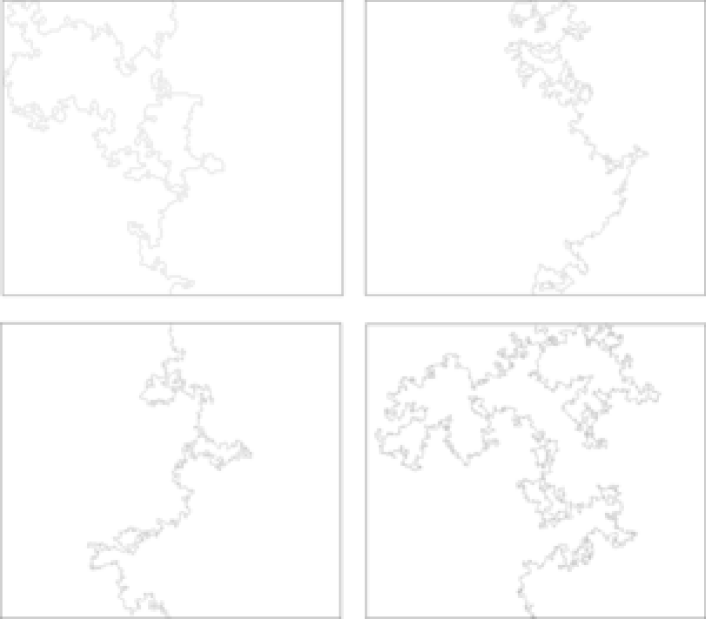
Figure 6: Samples of the harmonic navigator for increasing sizes.

We have also estimated the fractal dimension of the harmonic navigator. One finds a number close to $\delta=1.50\pm.01$. Again an accuracy of two significant digits can be achieved in a few hours of CPU. The computation time is of much longer than for percolation, and the ratio of the two does grows slowly when the size of the rectangular domain is changed. This is related to familiar properties of random walks : quite often, the random walk finds the boundary quickly, and hits it at a point nearby its starting point, most often at an hexagon bounding the growing interface. However, a look at the samples, obtained via the same pseudo random sequence but sharing only a modest initial portion, gives convincing evidence that from time to time, the walk hits the boundary far away from the interface. We shall come back to this later.

The study of the convergence, in the continuum limit, of the harmonic explorer to level lines in Gaussian (free) field theory and to SLE₄ (whose fractal dimension is exactly $3/2$) has seen important recent developments [120, 122].

The definition of the harmonic navigator can be extended in many directions.

The harmonic anti-navigator. Observe that if the neighborhood of an hexagon to be colored contains much more hexagons of one color than of the other, then with high probability it will get colored by the most abundant color. This means a repulsive force or excluded volume that tends to prevent the path from coming too close to another piece of itself. What if one decided to make the opposite color choice at each step? Then the resulting object would be much more dense, as confirmed by Fig.7 which shows a few samples in domains of increasing size.

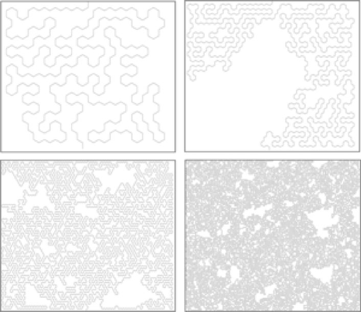
Figure 7: Samples of the harmonic anti-navigator for increasing sizes.

But does the harmonic anti-navigator have an interesting continuum limit? Is it related to conformal invariance?

The percolation navigator. What if we would replace the random walk by other processes that hit the boundary with probability 1 ? This means replacing the harmonic measure by another measure. For instance, we could start a percolation process at the tip of the growing interface, see the color of the boundary at the first hitting point and use this color for the new hexagon. It seems that nothing is known about this process. The samples in Fig.8 lead to expect nice fractals in the continuum limit. The fractal dimension can be estimated to be $\delta\sim 1.42$ and does not look like a simple number.

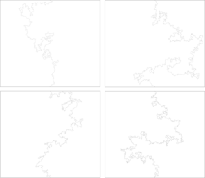
Figure 8: Samples of the percolation navigator for increasing sizes.

The boundary harmonic navigator. Yet another deformation of the harmonic navigator would be to keep only the initial boundary to compute the measure, i.e. let the interface be transparent to the random walk. In that case, the probability to color some hexagon in black or white depends only on the position of the hexagon, but not on the beginning of the interface. In fact one can color each inner hexagon by tossing a coin biased by the harmonic measure of the left and right boundaries seen from the hexagon. This leads to a statistical mechanics model with independent sites, and the probability of a given interface is just the product of the probabilities for all inner hexagons that have at least one edge on the interface. Hence, this process is similar to inhomogeneous percolation. The effect of the bias is a repulsive force away from the boundary of the initial domain and in the long range, the interfaces has a tendency to remain in regions where the bias is small and explore only a small part of the available space. On the other hand, in regions where the bias is small, at small scales the interface will look like percolation i.e. make many twists and turn. This is indeed the case, as shown on Fig.9. Due to the competition between small and large scales, conformal invariance is not expected. The CPU time needed to draw a sample is now much larger and grows faster when the size increases because the random walk has to explore space until it hits the initial boundary.

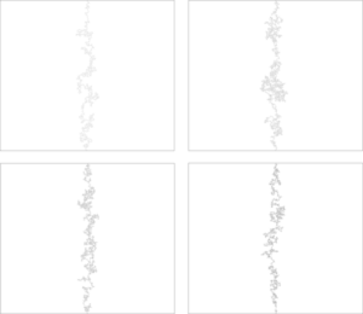
Figure 9: Samples of the boundary harmonic navigator for increasing sizes.

This is the first process that we meet for which removing the beginning of the path from the domain and starting the process for the cut domain at the tip is not the same as continuing the process in the initial domain. Thus this process does not have the so-called domain Markov property, an important feature of conformally invariant interfaces to which we shall come back later.

In fact all these variations –and many others– can be mixed. Deciding which one leads to a conformally invariant continuum limit is not so obvious. This illustrates that the landscape of plausible algorithms is vast and largely unexplored. There is room for numerical experiments and a lot of theoretical work.

2.1.3 Loop-erased random walks

This example still keeps some aspects of a growth process, in that new pieces of the process can be added recursively. A loop-erased random walk is a random walk with loops erased along as they appear. More formally, if $X_{0},X_{1},\cdots,X_{n}$ is a finite sequence of abstract objects, we define the associated loop-erased sequence by the following recursive algorithm.

Until all terms in the sequence are distinct,
Step 1 Find the couple $(l,m)$ with $0\leq l<m$ such that the terms with indexes from $0$ to $m-1$ are all distinct but the terms with indexes $m$ and $l$ coincide.
Step 2 Remove the terms with indexes from $l+1$ to $m$, and shift the indexes larger than $m$ by $l-m$ to get a new sequence.

Let us look at two examples.
For the “month” sequence j,f,m,a,m,j,j,a,s,o,n,d, the first loop is m,a,m, whose removal leads to j,f,m,j,j,a,s,o,n,d, then j,f,m,j, leading to j,j,a,s,o,n,d, then j,j leading to j,a,s,o,n,d where all terms are distinct.
For the “reverse month” sequence d,n,o,s,a,j,j,m,a,m,f,j, the first loop is j,j, leading to d,n,o,s,a,j,m,a,m,f,j, then a,j,m,a leading to d,n,o,s,a,m,f,j.

This shows that the procedure is not “time-reversal” invariant. Moreover, terms that are within a loop can survive: in the second example m,f, which stands in the j,m,a,m,f,j loop, survives because the first j is inside the loop a,j,m,a which is removed first.

A loop-erased random walk is when this procedure is applied to a (two dimensional for our main interest) random walk. In the full plane this is very easy to do. Fig.10 represents a loop-erased walk of 200 steps obtained by removing the loops of a 4006 steps random walk on the square lattice. The thin grey lines build the shadow of the random walk (where shadow means that we do not keep track of the order and multiplicity of the visits) and the thick line is the corresponding loop-erased walk. The time asymmetry is clearly visible and allows to assert with little uncertainty that the walk starts on the top right corner.

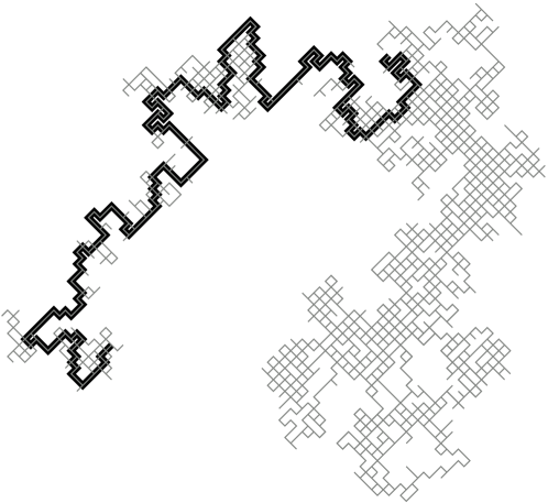
Figure 10: A loop-erased random walk with its shadow.

The same procedure can be applied to walks in the upper half plane. There are a few options for the choice of boundary conditions.
A first choice is to consider reflecting boundary conditions on the real axis for the random walk.
Another choice is annihilating boundary conditions: if the random walk hits the real axis, one forgets everything and starts anew at the origin. Why this is the natural boundary condition has to wait until Section 2.3.

Due to the fact that on a two-dimensional lattice a random walk is recurrent (with probability one it visits any site infinitely many times), massive rearrangement occur with probability one. This is already apparent on the small sample Fig.10 and means that if one looks at the loop-erased random walk associated to a given random walk, it does not have a limit in any sense when the size of the random walk goes to infinity. Let us illustrate this point. The samples in Fig.11 were obtained with reflecting boundary conditions. It takes 12697 random walk steps to build a loop-erased walk of length 633, but step 12698 of the random walk closes a long loop, and then the first occurrence of a loop-erased walk of length 634 is after 34066 random walk steps. Observe that in the mean time most of the initial steps of the loop-erased walk have been reorganized.

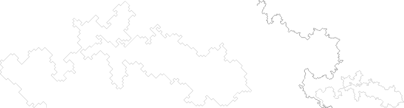
Figure 11: On the left: a large loop is about to be created. On the right: the massive rearrangement to go from 633 to 634 steps.

However, simulations are possible because when the length of the random walk tends to infinity, so does the maximal length of the corresponding loop-erased walk with probability one: there are times at which the loop-erased walk associated to a random walk will reach any number of steps $S$ ascribed in advance. If one stops the procedure the first time this happens, the random walk measure induces a measure on non-intersecting walks of $S$ steps which can be taken as a definition of the loop-erased random walk measure.

In a square lattice domain with admissible boundary condition $(\mathbb{D},a,b)$ we make the annihilating choice to define the loop-erased random walk measure. Consider all walks from $a$ to $b$ that do not touch the boundary except at $a$ before the first step and at $b$ after the last step and give each such walk of length $l$ a weight $4^{-l}$. Then erase the loops to get a probability distribution for loop-erased random walks from $a$ to $b$ in the domain. Observe that this choice is exactly the annihilating boundary condition. The probability for the simple symmetric random walk to hit the boundary for the first time at $b$ starting from $a$ can be interpreted as the partition function for loop-erased walks. A simple but expansive way to make simulations is to simulate simple random walks starting at $a$ and throw away those which hit the boundary before they leave at $b$.

Though annihilating boundary conditions lead to remove even more parts of the random walk than the reflecting ones, the corresponding process in the upper half plane can be arranged (conditioned in probabilistic jargon) to solve the problem of convergence as follows.

Instead of stopping the process when the loop-erased walk has reached a given length, one can stop it when it reaches a certain altitude, say $n$, along the $y$-axis. Whatever the corresponding random walk has been, the only thing that matters is the last part of it, connecting the origin to altitude $n$ without returning to altitude $0$. Moreover, the first time the loop-erased walk reaches altitude $n$ is exactly the first time the random walk reaches altitude $n$. Now a small miracle happens: if a 1d symmetric random walk is conditioned to reach altitude $n$ before it hits the origin again, the resulting walk still has the Markov property. It is a discrete equivalent to the 3d Bessel process (a Bessel process describes the norm of a Brownian motion, however no knowledge of Bessel processes is needed here, we just borrow the name). When at site m, $0<m<n$, the probability to go to $m\pm 1$ is $(1\pm 1/m)/2$, independently of all previous steps. Observe that there is no $n$ dependence so that we can forget about $n$, i.e. let it go to infinity. The discrete 3d Bessel process is not recurrent and tends to infinity with probability one: for any altitude $l$ there is with probability one a time after which the discrete 3d Bessel process remains above $l$ for ever. Henceforth, we choose to simulate a symmetric simple random walk along the $x$ axis and the discrete 3d Bessel process along the $y$-axis and we erase the loops of this new process. This leads to the convergence of the loop-erased walk and numerically to a more economical simulation.

Fig.12 is a simulation of about $10^{5}$ steps, both for reflecting and annihilating boundary conditions. At first glance, one observes in both cases similar simple (no multiple points) but irregular curves with a likely fractal shape. The intuitive explanation why a loop-erased random walk has a tendency not to come back too close to itself is that if it would do so, then with large probability a few more steps of the random walk would close a loop.

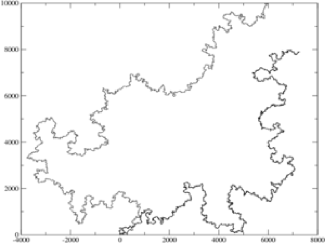
Figure 12: A sample of the loop-erased random walk for the two boundary conditions.

To estimate the Hausdorff dimensions in both cases, we have generated samples of random walks, erased the loops and made the statistics of the number of steps $S$ of the resulting walks compared to a typical length $L$ (end-to-end distance for reflecting boundary conditions, maximal altitude for annihilating boundary conditions). In both cases, one observes that $S\propto L^{\delta}$ and again a modest numerical effort (a few hours of CPU) leads to $\delta=1.25\pm.01$. This is an indication that the boundary conditions do not change the universality class.

To get an idea of how small the finite size corrections are, observe Fig.13. The altitude was sampled from $2^{4}$ to $2^{13}$. The best fit gives a slope $1.2496$ and the first two points already give $1.2403$.

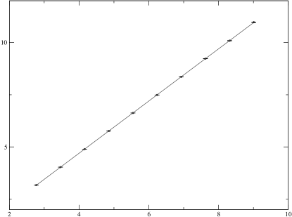
Figure 13: The logarithm of the average length of the loop-erased random walk versus logarithm of the maximum altitude. The numerical results are the circles, the straight line is the linear regression, the error bars are shown.

As recalled in the introduction, it is believed on the basis of intuitive arguments that in two dimensions scale invariance is almost enough for conformal invariance, providing there are no long range interactions. What does this absence of long range interactions mean for loop-erased random walks? Clearly along the loop-erased walk there are long range correlations, if only because a loop-erased random walk cannot cross itself. A possibly more relevant feature is that, in the underlying 2d physical space, interactions are indeed short range. At each time step, the increment of the underlying random walk is independent of the rest of the walk, and the formation of a loop to be removed is known from data at the present position of the random walk.

From the analytical viewpoint, the loop-erased random walk is one of the few systems that has been proved to have a conformally invariant distribution in the continuum limit, the fractal dimension being exactly $5/4$. A naive idea to get directly a continuum limit representation of loop-erased walks would be to remove the loops from a Brownian motion. This turns out to be impossible due to the proliferation of overlapping loops of small scale. However, the SLE₂ process, to be defined later, gives a direct definition. In fact, it is the consideration of loop-erased random walks that led Schramm [118] to propose SLE as a description of interfaces.

2.1.4 SAW

The self avoiding walk is one of the most important examples, and it is known to lead to notoriously difficult questions. One of the reasons is perhaps that a recursive definition is not known. And it is likely that before the discovery of SLE few people would have bet that the continuum limit of self avoiding walks would be described most naturally as a (Markovian!) growth process.

The statistical ensemble of self avoiding walks of $S$ steps can be defined on an arbitrary simple graph. The probability space consists of sequences of $S+1$ distinct adjacent vertices, and if not empty, it is endowed with the uniform probability measure. Conditioning on the initial and/or the end point leads to other ensembles, again with uniform probability distribution. We are interested mainly in the case when the graph is a simply connected piece of a 2-d lattice. One of the difficulty is that if $S=S^{\prime}+S^{\prime\prime}$ the $S^{\prime}$ first steps obviously build a self avoiding walks of length $S^{\prime}$ but the number of possible complements of length $S^{\prime\prime}$ depends on the first $S^{\prime}$ steps, so that the induced probability measure on the $S^{\prime}$ first steps obtained by summing over the last $S^{\prime\prime}$ steps is not uniform. So it is tricky to produce samples of self avoiding walks by a recursive procedure. In fact the most efficient way known at present to simulate self avoiding walks is via a dynamical Monte Carlo algorithm.

Let us pause for a second to recall the basic idea. To produce samples of a finite probability space $\Omega=\{a,b,c,\cdots\}$ (which we can assume to give a positive probability to each of its points), the starting point of a dynamical Monte Carlo algorithm is to view the points in the probability space as vertices of an abstract graph. The task is then to define enough edges to make a connected graph and cook up for each edge $\{a,b\}$ two oriented weights $z_{ab}$ to go from point $a$ to point $b$ and $z_{ba}$ to go from $b$ to $a$ in such a way that $p_{a}z_{ab}=p_{b}z_{ba}$ (detailed balance). Then a random walk on the graph using the weights $z_{ab}$, with arbitrary initial conditions, leads at large times to a stationary distribution which is exactly the probability distribution one started with. The art is in a clever choice of edges, also called elementary moves. The complete graph is most of the time not an option, not only for size questions. The point is that quite often $\Omega$ is hard to describe even if the probability law itself is simple (even uniform) because $\Omega$ lacks structure. But even in that situation, one can often guess simple choices of elementary moves and show that they are enough to ensure connectivity. This can be much easier than an enumeration of $\Omega$.

The simulation of self avoiding walks is a famous example of this strategy. On a regular lattice, a convenient choice of moves is given by so called “pivots” which we describe briefly, [127, 76]. To have a finite sample space of non-intersecting walks, fix their length and initial point. Let us describe a time step. Starting from any non-intersecting walk, at each step choose a vertex (called the pivot) on the walk and a lattice symmetry fixing the pivot, both with the uniform probability. Keep the part of the walk before the pivot, but apply the symmetry to the part of the walk after the pivot. If the resulting walk intersects itself, do nothing. Else move to the new walk. Decide that two non-intersecting walks are connected if one can go from one to the other in a time step. It is not too difficult to show that the resulting graph on non-intersecting walks is connected and that detailed balance holds for the uniform probability distribution on non-intersecting walks. Hence the stationary long time measure for the pivot Monte Carlo algorithm is the self avoiding walk measure.

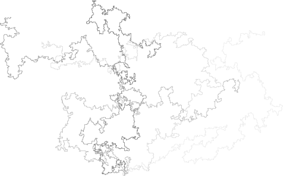
Figure 14: A few self avoiding walks.

Fig.14 shows a few samples. Producing a single clean sample of reasonable size starting from a walk far from equilibrium (like a straight segment) takes many Monte Carlo iterations. In fact it takes roughly the time needed to compute the fractal dimension with 1 percent error for our previous examples. However, once the large time regime is reached, one estimates that only a fraction of the number of iterations needed to thermalize is enough to get a new (almost) independent sample, so that a good numerical estimate of the fractal dimension of the self avoiding walk can still be obtained via a modest numerical effort. Thinking about the way samples are build, it may seem hard to believe that the self avoiding walk can be viewed as a growth process in a natural way, which is what SLE does.

In some respect the self avoiding walk is in a position similar to the one of percolation because it has a compelling characteristic property. Percolation has locality, and the self avoiding walk has the restriction property. If a sample space is endowed with the uniform probability measure and one concentrates on a subspace (or, in probabilistic language, conditions on a subspace) the measure induced on the subspace is obviously still uniform. Hence the self avoiding walk on a graph conditioned not to leave a certain subgraph is the self avoiding walk on the subgraph. This is called restriction. As we shall see later, among SLE_κ’s, SLE_8/3 is the only one that satisfies restriction. So if the continuum limit of the self avoiding walk exists and is conformally invariant –two facts which are still conjectural at the moment despite hard efforts of gifted people– it has to be SLE_8/3 and the value of its fractal dimension, $4/3$, comes for free.

It is also useful to consider ensembles of self avoiding walks of variable length. In the full plane, the logarithm of the number of self avoiding walks of $S$ steps is $\sim S\log\mu$ for large $S$ where $\mu$ is lattice dependant. To get a continuum limit made of long fluctuating walks, it is thus necessary to weight each self avoiding walk with weight $\mu^{-S}$.

We hope that these examples have convincingly supported our assessment in the introduction that the world of interfaces and of algorithms to explore it is incredibly rich and wide, harvesting many beautiful and fragile objects.

2.2 Examples from statistical mechanics

2.2.1 Ising model

Our first example from statistical mechanics is the celebrated Ising model, where we choose to put the spin variables on the faces of an hexagonal lattice domain with admissible boundary conditions $(\mathbb{D},a,b)$ and we use the low temperature expansion. The spins are fixed to be $up$ on the left and $down$ on the right faces. The energy of a configuration is proportional to the length of the curves separating up and down islands. There is one interface from $a$ to $b$ and a number of loops, see Fig.15.

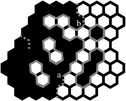
Figure 15: A configuration of the Ising model.

The proportionality constant in the configuration energy has to be adjusted carefully to lead to a critical system with long range correlations. This time, making accurate simulations is much more demanding. On the square lattice, the definition of the interface suffers from ambiguities, but these become less relevant for larger sample sizes. Fig.16 is an illustration.

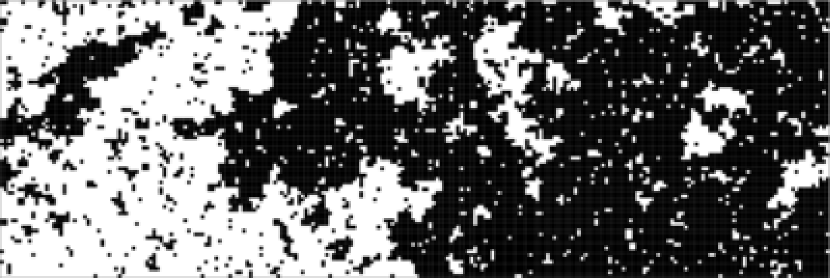
Figure 16: A sample for the critical Ising model. The bottom line, where the spins are frozen –black on the right, white on the left– is not represented. Courtesy of J. Houdayer.

Although there is no question that the fractal dimension of the Ising interface with the above boundary conditions is $11/8$ and is described by the –to be defined later– SLE₃ ensemble, a mathematical proof that a continuum limit distribution for the interface exists and is conformally invariant is still out of reach.

2.2.2 Potts models

The $Q$-state Potts model can be defined on an arbitrary simple graph $G=(V,E)$ with vertices $v\in V$ and edges $\{v,v^{\prime}\}\in E\subset\mathrm{sym}(V^{2})$, the collection of two-elements subsets of $V$. The parameter $Q$ is a positive integer to start with. Each vertex $v\in V$ carries a variable $S_{v}\in\{1,\cdots,Q\}$. The Boltzmann weight of a configuration is by definition

$$\prod_{\{v,v^{\prime}\}\in E}e^{\beta(\delta_{S_{v},S_{v^{\prime}}}-1)},$$

where $\beta>0$ is the temperature. Write $e^{\beta(\delta_{S_{v},S_{v^{\prime}}}-1)}=p\delta_{S_{v},S_{v^{\prime}}}+(1-p)$ where $p\equiv 1-e^{-\beta}\in[0,1]$, view the first term, $p\delta_{S_{v},S_{v^{\prime}}}$, as “the edge $\{v,v^{\prime}\}$ is occupied”, the second term as “the edge $\{v,v^{\prime}\}$ is not occupied” and expand the Boltzmann weight as a sum of $2^{|E|}$ terms. Each term is associated to a subgraph $C$ of $G$ with the same vertex set $V$, but edges in $E_{C}$, the subset of $E$ made of the occupied edges. The partition function $Z$ is obtained by summing each of the $2^{|E|}$ terms over the $Q^{|V|}$ spin configurations. Each connected component of $C$ gives a non vanishing factor only if all spins in it are the same. Hence, each cluster (=connected component) of $C$ gives a factor $Q$ (isolated points count as clusters) and the partition function can be rewritten, following Fortuin-Kastelyn [61], as a sum over cluster configurations

$$Z=\sum_{C}\,p^{|E_{C}|}\,(1-p)^{|E|-|E_{C}|}\,Q^{N_{C}}$$

where $N_{C}$ the number of clusters in the configuration $C$. This formula makes sense for arbitrary $Q$ now.

To introduce interfaces, one can consider for instance that the vertices of the graph on which the Potts model is defined are the faces of an hexagonal lattice domain. Freeze the left faces to a given color, so that a left cluster containing all left faces (plus possibly some other) can be defined and either freeze the right vertices at a different value, see Fig.17 for an illustration, or condition on configurations such that the left cluster does not contain right faces. There is a single simple lattice path bounded on the left by the left cluster, and it defines an interface. If the hexagons of the left cluster are colored black and the other ones white, the interface separates the two colors.

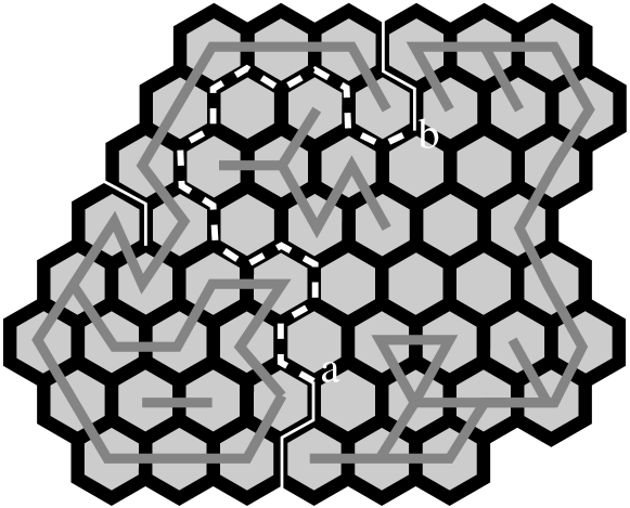
Figure 17: FK-clusters configuration in the Potts models and the corresponding interface.

For $Q\leq 4$ the parameter $p$ can be adjusted so that a continuum scale invariant limit exists. The interface is conjectured to be conformally invariant and statistically equivalent to an SLE trace [118, 115].

For $Q=2$, the Potts model Boltzmann weight is proportional to the Ising model weight, and for general $Q$, again up to a constant, the energy is given by the length of the curves separating islands of identical spins. However, when $Q>2$, these curves are complicated and not very manageable. This is related to the following fact. The reader will have noticed that we always choose situations when the lattice interface is a simple curve. This is needed to be in the SLE framework, but this is not a generic situation. For instance the physical interface separating clusters of different colors in the $Q=3$ Potts model do exhibit points where three lines meet, loops et cætera.

2.2.3 $O(n)$ models

The $O(n)$ model can also be defined on an arbitrary simple graph $G=(V,E)$ with vertices $v\in V$ and edges $\{v,v^{\prime}\}\in E\subset\mathrm{sym}(V^{2})$. This time each vertex $v\in V$ carries a variable $\sigma_{v}=(\sigma_{v}^{1},\cdots,\sigma_{v}^{n})\in S^{n-1}$, the sphere in $n$ dimensions with radius $\sqrt{n}$. The measure $d\mu$ is the rotation invariant measure of unit mass on that sphere, so that

$$\int d\mu(\sigma)=1\quad\int d\mu(\sigma)\sigma^{\alpha}\sigma^{\beta}=\delta^{\alpha\beta},$$

while the integrals of odd functions of $\sigma$ vanish.

The Boltzmann weight of a configuration is

$$\prod_{\{v,v^{\prime}\}\in E}w(\sigma_{v}\cdot\sigma_{v^{\prime}}),$$

where $\sigma_{v}\cdot\sigma_{v^{\prime}}\equiv\sigma_{v}^{1}\sigma_{v^{\prime}}^{1}+\cdots+\sigma_{v}^{n}\sigma_{v^{\prime}}^{n}$ is the scalar product. In the original version of the model, $w(x)=e^{\beta x}$, but for certain classes of graphs, there is a more convenient choice to which we shall come in a moment.

We start by defining the graph associated to an hexagonal lattice domain $\mathbb{D}$. We forget the open hexagons and only keep the edges and vertices in $\mathbb{D}$. Then we add the vertices needed to get a closed set in the plane, yielding the desired (planar) graph $G_{\mathbb{D}}$. Note that $\mathbb{D}$ can be recovered from $G_{\mathbb{D}}$ by adding the open hexagons needed to have each edge bounded on both sides, and then taking the topological interior to remove the unwanted vertices.

One good property of this class of graphs is that it is a subclass (that we do not try to characterize) of the class of graphs with vertices of valence at most three. A boundary vertex is by definition a vertex of valence $<3$. On such graphs, it is convenient to choose $w(x)=1+tx$ where $t$ is a parameter. The Boltzmann weight is $\prod_{\{v,v^{\prime}\}\in E}(1+t\,\sigma_{v}\cdot\sigma_{v^{\prime}})$.

To get a graphical representation of the partition function, expand the Boltzmann weight as a sum of monomials in the $\sigma_{v}\cdot\sigma_{v^{\prime}}$’s. Each monomial corresponds to a subgraph of $G$. Then integrate each monomial against $\prod_{v\in V}d\mu(\sigma_{v})$. Each $\sigma_{v}$ appears at most three times in a monomial, so that the trivial integrals listed above allow to compute everything. A monomial gives a nonzero contribution if and only if the subgraph it describes is a union of disjoint cycles, also called loops. Call such a subgraph a loop subgraph of $G$. Then

$$Z=\sum_{F\in\mathcal{F}}n^{l(F)}t^{b(F)},$$

where $F$ runs over all loop subgraphs of $G$, $l(F)$ is the number of loops of $F$ and $b(F)$ is the number of bonds (i.e. edges) in $F$. So we are summing over a loop gas. The temperature-like parameter $t$ can be reinterpreted as a bond fugacity.

Interfaces appear in a natural way via correlation functions. There are several options and we shall use the simplest: choose a component number, say $1$, and insert $\sigma^{1}$’s at boundary vertices $v_{1},\cdots,v_{2k}$. The insertion of an odd number of $\sigma^{1}$’s gives $0$. Up to now, we have mostly considered the case $k=1$ when only one interface is present. Again, $Z_{v_{1},\cdots,v_{2k}}\equiv Z\langle\sigma_{v_{1}}^{1}\cdots\sigma_{v_{2k}}^{1}\rangle$ has a graphical expansion as a sum over $\mathcal{F}_{v_{1},\cdots,v_{2k}}$, the collection of subgraphs of $G$ consisting on the one hand of $k$ connected component which are (simple) lines pairing the insertion points and on the other hand of an arbitrary number of connected component which are loops. Again, each loop gives a factor $n$, but the lines give a factor $1$. Explicitly,

$$Z_{v_{1},\cdots,v_{2k}}=\sum_{F\in\mathcal{F}_{v_{1},\cdots,v_{2k}}}n^{l(F)}t^{b(F)}.$$

Alternatively we could choose several component numbers (if $n$ is large enough). Then each component number has to appear an even number of times to give a non-vanishing result, and then different kinds of lines appear, pairing insertion points with the same component numbers. Note that this can be seen as a conditioning of the previous situation.

We could also look at correlators which are scalar products, yielding slightly different rules to weight the lines, depending whether they connect two insertions which build a scalar product or not.

Up to now, we have seen the graphical expansion as a trick to study the original spin model, which could be formulated only for integral $n$. However, the graphical expansion gives a meaning when $n$ is a formal parameter, in particular a real or complex number. The general model is interesting for its own sake. For instance, one can introduce conditioning. One can restrict the sums over subgraphs which contain all vertices of $G$, leading to so-called fully packed models. One can also impose say that a given bulk lattice point belongs to an interface, and we would like to interpret the corresponding partition function as a correlator with a certain field inserted at that point. The price to pay for such extensions is that the original local Boltzmann weight is replaced by nonlocal weights. We shall see later that nevertheless the $O(n)$ model for general $n$ still has a very important property, the domain Markov property.

Take an hexagonal lattice domain $\mathbb{D}$ and choose a “loops and lines” configuration for $G_{\mathbb{D}}$. If one associates a $+$ sign to an arbitrary hexagon of $\mathbb{D}$ there is a single way to extend this assignment to all hexagons of $\mathbb{D}$ by continuity, flipping the sign only when a loop or a line is crossed. So there is another version of the configuration space using Ising like variables. A “loops and lines” configuration can be seen as the frontier between island of opposite signs.

For $n=1$, we recover that Kramers-Wannier duality between the low temperature expansion of the Ising model for spins on the faces of $\mathbb{D}$ that we studied before and the high temperature expansion of the Ising model for spins on the vertices of $G_{\mathbb{D}}$.

Note also that for $n=0$ one recovers the correct weight for self-avoiding walks as introduced before. This is another illustration that the physical approach via statistical mechanics and the mathematical approach via combinatorics are in fact closely related.

Considering the previous superficial remarks, it is probably not surprising that the phase structure of $O(n)$ models is rather complicated and interesting. when $n\in[-2,2]$, one can adjust $t$ so that a continuum scale invariant limit exists. The interface is again conjectured to be conformally invariant and statistically equivalent to an SLE trace.

2.3 The domain Markov property

We have already insisted that the models of interfaces should be defined on lattice domains of arbitrary shapes. Let us however note that the possibility to have a natural definition on arbitrary lattice domains is not so obvious. For models of geometric interfaces, there is no general recipe, and for specific cases we have taken a definition which may look arbitrary, as illustrated by the loop erased random walk example. For statistical mechanics, the models we have introduced have a natural definition on any domain because they are based on nearest neighbor interactions and need only an abstract graph structure.
Suppose that $(\mathbb{D},a,b)$ is a lattice domain with admissible boundary condition and $\gamma_{[ab]}\equiv(s_{1},\cdots,s_{2n+1})$ is a path from $a$ to $b$ in $\mathbb{D}$. Recall that this means that $a=s_{1},b=s_{2n+1}$, the odd $s_{2m+1}$, $1\leq m<n$, (if any) are distinct vertices of the decomposition of $\mathbb{D}$ and the even $s_{2m}$, $1\leq m<n$, are distinct edges of the decomposition of $\mathbb{D}$ with boundary $\{s_{2m-1},s_{2m+1}\}$. We use $P_{(\mathbb{D},a,b)}$ to denote the probability distribution for the interface $\gamma_{[ab]}$ from $a$ to $b$ in $\mathbb{D}$.

Choose an integer $m$ such that $0\leq m<n$ and set $s_{2m+1}\equiv c$. Decompose $\gamma_{[ab]}=\gamma_{[ac]}\cdot\gamma_{[cb]}$, where the $\cdot$ means concatenation. The set $\mathbb{D}^{\prime}\equiv\mathbb{D}\setminus\gamma_{]ac]}$, obtained by cutting along $\gamma_{[ac]}$ with scissors, i.e. by removing from $\mathbb{D}$ the sets $s_{l}$, $1<l\leq s_{2m+1}$, is still a domain, and $(c,b)$ is an admissible boundary condition for $\mathbb{D}^{\prime}$. Hence we can compare two things.
1) The probability in $(\mathbb{D},a,b)$ of $\gamma_{[ab]}$ conditioned to start with $\gamma_{[ac]}$, that is the ratio of the probability of $\gamma_{[ab]}$ by the probability for the interface to start with $\gamma_{[ac]}$.
2) The probability of $\gamma_{[bc]}$ in $(\mathbb{D}^{\prime},c,b)$. This is illustrated on Fig.18.

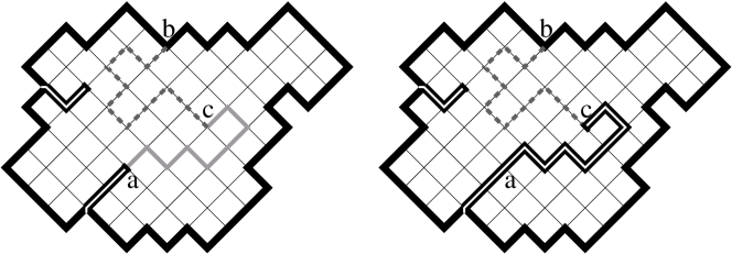
Figure 18: An illustration of situations 1) and 2) for the case of loop-erased walks. What is the distribution of the dotted curve in both situations ?

The domain Markov property is the statement that these two probabilities are equal. In equations

$$P_{(\mathbb{D},a,b)}(\;.\;|\gamma_{[ac]})=P_{(\mathbb{D}\setminus\gamma_{]ac]},c,b)}(\;.\;).$$

All the examples of interfaces introduced so far have the domain Markov property, but for a single exception. First, it is obvious that these two probabilities are supported on the same set, namely simple curves along the edges of the lattice, going from $c$ to $b$ in $\mathbb{D}\setminus\gamma_{]ac]}$. Let us however note that for loop-erased random walks, annihilating boundary conditions are crucial. Reflecting boundary conditions clearly do not work, if only because the supports do not coincide in that case.

– For percolation, the domain Markov property is seen directly by using the definition of percolation as a growth process.

– For the harmonic navigator, the domain Markov property rests on the fact that the random walk can go not only on the initial boundary but also on the beginning of the interface. This is still true of the variants that we introduced, except the one we called the boundary harmonic navigator, when we imposed that the initial part of the interface be transparent and the random walk could accost only the initial boundary.

– For the case of the loop erased walk a little argument is needed. Take any random walk (possibly with loops) $W_{0}=a,W_{1},\cdots,W_{l}=b$ that contributes to an interface $\gamma_{[ab]}$ which is $\gamma_{[ac]}$ followed by some $\gamma_{[cb]}$. Let $m$ be the largest index for which the walk visits $c$. Because the interface has to start with $\gamma_{[ac]}$, the walk $W_{m}=c,\cdots,W_{l}=b$ cannot cross $\gamma_{[ac[}$ again, so it is in fact a walk in $\mathbb{D}\setminus\gamma_{[ac[}$ from $c$ to $b$ leading to the interface $\gamma_{[cb]}$. The weight for the walk $W_{0}=a,W_{1},\cdots,W_{l}=b$ is $4^{-l}$, i.e. simply the product of weights for the walks $W_{0}=a,W_{1},\cdots,W_{m}=c$ and $W_{m}=c=a,\cdots,W_{l}=b$. Then a simple manipulation of weights leads directly to the announced result.

– The domain Markov property for the self avoiding walk rests (just like the restriction property) on the fact it endows non-intersecting walks with the uniform probability measure. Then the self avoiding walk measure conditioned on the beginning of the interface is still uniform, so it is the self avoiding walk measure on the cut domain.

– For the statistical mechanics model, in fact more is true: we can view $P_{(\mathbb{D},a,b)}$ not only as a probability distribution for the interface, but as the full probability distribution for the full configuration space and still check the identity of 1) and 2). For orientation, first restrict attention to the O(n) model when $n$ is an integer. The supports are the same for 1) and 2), namely any configuration of the colors, except that the colors on both sides of $\gamma_{[ac]}$ are fixed. The Boltzmann weight involves only nearest neighbor interactions. The conditional probability in 1) takes into account the interactions between the colors along the interface $\gamma_{[ac]}$, whereas the probability in 2) does not take into account the interactions between the colors along the cut left by the removal of $\gamma_{]ac]}$. However, the corresponding colors are fixed anyway, so the Boltzmann weights for the configurations that are in the support of 1) or 2) differ by an overall multiplicative constant, which disappears when probabilities are computed.
This argument extends immediately to systems with only nearest neighbor interactions. They can be defined on any graph. If any subset of edges is chosen and the configuration at both end of each edge is frozen, it makes no difference for probabilities to consider the model on a new graph in which the frozen edges have been deleted.
When $Q$ (Potts model) or $n$ ($O(n)$ model) are not integers, the Boltzmann weights are not local anymore, but again the Boltzmann weights for the configurations that are in the support of 1) or 2) differ by an overall multiplicative constant, related to the length of $\gamma_{[ac]}$, which disappears when probabilities are computed.

The domain Markov property –which, as should be amply evident, has nothing to do with conformal invariance– together with the conformal invariance assumption is at the heart of O. Schramm’s derivation of stochastic Loewner evolutions.

We end our discussion of the domain Markov property by an illustration of its predictive power. We have seen on the example of the $O(n)$ model that dealing with several interfaces is easy in the framework of statistical mechanics. What about trying to define directly several interfaces, say two, for loop erased random walks for instance? We want that one goes from $a$ to $b$ and the second from $a^{\prime}$ to $b^{\prime}$. We shall sum over pairs of random walks, but how should we restrict the sum. Should the random walks avoid each other, or should they simply be such that the associated loop erased walk avoid each other. If the domain Markov property is to be preserved, the answer is neither. The recipe can be nothing but the following: build the first loop erased walk $\gamma_{[a,b]}$ from $a$ to $b$ in $\mathbb{D}$ and cut the domain in two pieces, keep only the piece $\mathbb{D}^{\prime}_{\gamma_{[a,b]}}$ that contains $a^{\prime}$ and $b^{\prime}$ and then build the second loop erased walk from $a^{\prime}$ to $b^{\prime}$ in the sub-domain. The recipe looks asymmetric: for $\gamma_{[a,b]}$ we sum over walks in $\mathbb{D}$, but for $\gamma_{[a^{\prime},b^{\prime}]}$ we sum over walks in $\mathbb{D}^{\prime}_{\gamma_{[a,b]}}$. Let $S$ be this sum. Write $S=S^{\prime}-S^{\prime\prime}$ where $S$ is the sum over all couples of random walks (which is symmetric), and $S^{\prime}$ is the sum of couples of random walks such that the walk from $a^{\prime}$ to $b^{\prime}$ hits $\gamma_{[a,b]}$. Now split $S^{\prime\prime}=S^{\prime\prime\prime}+S^{\prime\prime\prime\prime}$ where $S^{\prime\prime\prime}$ is the sum over couples of random walks such that the each one touches the other loop erased walk (which is symmetric), and $S^{\prime\prime\prime\prime}$ is the sum over couples of random walks such that the one from $a$ to $b$ does not touch $\gamma_{[a^{\prime},b^{\prime}]}$ but the one from $a^{\prime}$ to $b^{\prime}$ does touch $\gamma_{[a,b]}$. Then removes the loops that hit $\gamma_{[a,b]}$ on the walk from $a^{\prime}$ to $b^{\prime}$ to graft them in the appropriate order on the walk from $a$ to $b$ and to see that $S^{\prime\prime\prime\prime}$ is in fact symmetric. This is closely related to the general definition of multiple SLE’s, either by imposing commutativity [48] or by imposing properties natural from the viewpoint of statistical mechanics [14].

2.4 Other growth processes

Previous examples, either geometrical or extracted from statistical mechanic models, are actually static. The growth dynamics arises – or will arise soon in the following Sections – only via the way we choose to described them. The fact that such dynamical description of static objects is efficient is tided to their conformal properties. There are however a large class of truly growth processes specifying the dynamics of fractal domains. The most famous is diffusion limited aggregation (DLA) which described successive aggregations of tiny particles. Since DLA only assumed that the growth is governed by diffusion its domain applicability – for instance to aggregation or deposition phenomena – is quite large. Of course many works, experimental, numerical or theoretical, have been devoted to DLA, see refs.[22, 65, 68, 18, 130, 129] for alternative reviews and extra references. We shall not review all of them but only have a glance on that field. Another standard example, the so-called Hele-Shaw problem, has an hydrodynamic origin [22, 117, 37]. It may be viewed as describing the invasion of an oil domain by an air bubble. Its dynamics leads to very interesting formation of domains with finger-like shapes which are non-linearly selected [123, 38]. It is one of the basics models of non-linear pattern formations and selections. Both, DLA and Hele-Shaw, are related to Laplacian growth (LG), see eg.[22].

2.4.1 DLA

DLA stands for diffusion limited aggregation [141]. It refers to processes in which the domains grow by aggregating diffusing particles. Namely, one imagines building up a domain by clustering particles one by one. These particles are released from the point at infinity, or uniformly from a large circle around infinity, and diffuse as random walkers. They will eventually hit the domain and the first time this happens they stick to it. By convention, time is incremented by unity each time a particle is added to the domain. Thus at each time step the area of the domain is increased by the physical size of the particle. The position at which the particle is added depends on the probability for a random walker to visit the boundary for the first time at this position.

In a discrete approach one may imagine that the particles are tiny squares whose centers move on a square lattice whose edge lengths equal that of the particles, so that particles fill the lattice when they are glued together. The center of a particle moves as a random walker on the square lattice. The probability $Q(x)$ that a particle visits a given site $x$ of the lattice satisfies the lattice version of the Laplace equation $\nabla^{2}Q=0$. It vanishes on the boundary of the domain, i.e. $Q=0$ on the boundary, because the probability for a particle to visit a point of the lattice already occupied, i.e. a point of the growing cluster, is zero. The local speed at which the domain is growing is proportional to the probability for a site next to the interface but on the outer domain to be visited. This probability is proportional to the discrete normal gradient of $Q$, since the visiting probability vanishes on the interface. So the local speed is $v_{n}=(\nabla Q)_{n}$. It is not so easy to make an unbiased simulation of DLA on the lattice. One of the reasons is that on the lattice there is no such simple boundary as a circle, for which the hitting distribution from infinity is uniform. The hitting distribution on the boundary of a square is not such a simple function. Another reason is that despite the fact that the symmetric random walk is recurrent is 2d, each walk takes many steps to glue to the growing domain. The typical time to generate a single sample of reasonable size with an acceptable bias is comparable to the time it takes to make enough statistics on loop-erased random walks or percolation to get the scaling exponent with two significant digits. Still this is a modest time, but it is enough to reveal the intricacy of the patterns that are formed. Fig.19 is such a sample.

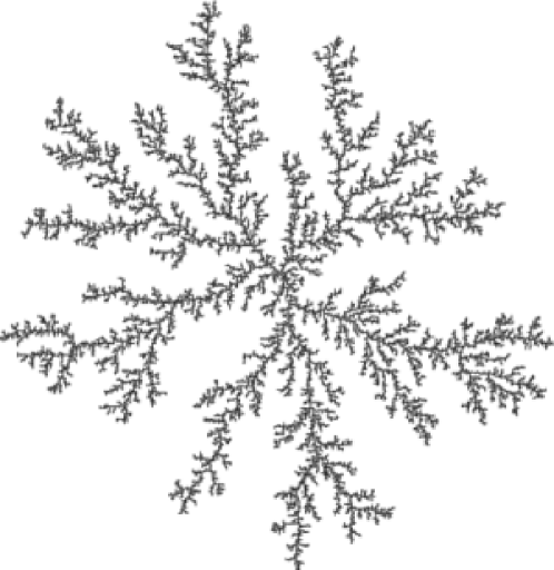
Figure 19: A DLA sample.

During this process the clustering domain gets ramified and develops branches and fjords of various scales. The probability for a particle to stick on the cluster is much higher on the tip of the branches than deep inside the fjords. This property, relevant at all scales, is responsible for the fractal structure of the DLA clusters.

Since its original presentation [141], DLA has been studied numerically quite extensively. There is now a consensus that the fractal dimension of 2d DLA clusters is $D_{\rm dla}\simeq 1.71$. There is actually a debate on whether this dimension is geometry dependent but a recent study [128] seems to indicate that DLA clusters in a radial geometry and a channel geometry have identical fractal dimension. To add a new particle to the growing domain, a random walk has to wander around and the position at which it finally sticks is influenced by the whole domain. To rephrase this, for each new particle one has to solve the outer Laplace equation, a non-local problem, to know the sticking probability distribution. This is a typical example when scale invariance is not expected to imply conformal invariance.

2.4.2 Laplacian growth and others

DLA provides a discrete analogue of Laplacian growth. The particle size plays the role of an ultraviolet cutoff. Laplacian growth is a process in which the growth of a domain is governed by the solution of Laplace equation, i.e. by an harmonic function, in the exterior of the domain with appropriate boundary conditions. It has many interpretation either in terms of aggregation of particles as in DLA but also in hydrodynamic terms (then the solution of Laplace equation is the pressure) or electrostatic terms (then the solution is the electrostatic potential).

To be a bit more precise [22], let $P$ be the real solution of Laplace equation, $\nabla^{2}P=0$, in the complement of an inner domain in the complex plane with the boundary behavior $P=-\log|z|+\cdots$ at infinity and $P=0$ on the boundary curve. The time evolution of the domain is then defined by demanding that the normal velocity of points on the boundary curve be equal to minus the gradient of $P$: $v_{n}=-(\nabla P)_{n}$.

One may also formulate Laplacian growth using a language borrowed from electrostatics by imagining that the inner domain is a perfect conductor. Then $V=\Re{\rm e}\,\Phi_{t}$ is the electric potential which vanishes on the conductor but with a charge at infinity. The electric field $\vec{E}=\vec{\nabla}V$ is $\bar{E}\equiv E_{x}-iE_{y}=\partial_{z}\,\Phi_{t}$. Its normal component $E_{n}=|f_{t}^{\prime}(u)|^{-1}$ is proportional to the surface charge density. A slight generalization of this model to be discussed in Section 8.2 leads to a model of dielectric breakdown [107].

In the hydrodynamic picture, one imagines that the inner domain is filled with a non viscous fluid, say air, and the outer domain with a viscous one, say oil. Air is supposed to be injected at the origin and there is an oil drain at infinity. The pressure in the air domain is constant and set to zero by convention. In the oil domain the pressure satisfies the Laplace equation $\nabla^{2}P=0$. If we neglect the surface tension, then pressure vanishes on the boundary curve and the model is equivalent to Laplacian growth. In presence of surface tension then the pressure on the boundary condition is $P=-\sigma\kappa$ with $\sigma$ the surface tension and $\kappa$ the curvature of the boundary curve. This is the so-called Hele-Shaw problem. For non zero surface tension, it provides a regularization of Laplacian growth. There are nice experiences on these systems [129].

Besides DLA, another class of discrete growth processes are theoretically defined by iterating conformal maps. The similarity with the sample in Fig.38 obtained by this method and that obtained by aggregation, Fig.19, is striking. But a quantitative comparison of the two models is well out of analytic control and belongs to the realm of extensive simulations. We shall described them at the end of this review, see Section 8.4.

All these models involve very nice pattern formations. Their relations with Loewner chains will be described in Section 8, but it is already clear that their solutions involve analytic functions and that there are challenging physics and mathematics behind these problems.

3 Loewner chains

The description of Loewner chains and SLE processes is based on coding domain shapes in conformal maps using techniques – especially Riemann theorem – from basic theory of analytical functions that we recall briefly in this Section. More details may of course be found in standard references [39, 2] on analytic functions.

3.1 Conformal mappings

A domain is a non empty connected and simply connected open set strictly included in the complex plane $\mathbb{C}$. Simple connectedness is a notion of purely topological nature which in two dimensions asserts essentially that a domain has no holes and is contractible: the domain has the same topology as a disc. But it is a deep theorem of Riemann that two domains are always conformally equivalent, i.e. there is an invertible holomorphic map between them. These maps are usually called uniformizing maps. For instance, the upper-half plane $\mathbb{H}$ and the unitary disc $\{z\in\mathbb{C},|z|<1\}$ centered on the origin are two domains. The conformal transformation $f(z)=i\frac{1-z}{1+z}$ maps the unitary disc onto the upper half plane with $f(0)=i$ and $f(1)=0$.

It is well known that the upper half plane has a three dimensional Lie group of conformal automorphisms, $PSL_{2}(\mathbb{R})$, that also acts on the boundary of $\mathbb{H}$. This group is made of homographic transformations $f(z)=\frac{az+b}{cz+d}$ with $a,b,c,d$ real and $ad-bc=1$. To specify such map we have to impose three real conditions. Hence, there is a unique automorphism – possibly followed by a transposition – that maps any triple of boundary points to any other triple of boundary points. Similarly there is unique homographic transformation that maps any pair made of a bulk point and a boundary point to another pair of bulk and boundary points. By Riemann’s theorem, this is also true for any other domain – at least if the boundary is not too wild – so that uniformizing maps are fully specified once three conditions have been imposed.

Riemann’s theorem is used repeatedly in the rest of this review. It is the starting point of many approaches to growth phenomena in two dimensions since it allows to code the shapes of growing domains in their uniformizing conformal maps. To make the description precise one has to choose a reference domain against which the growing domains are compared. Again by Riemann theorem we may choose any domain as reference domain – and depending on the geometry of the problem some choices are simpler than others. To simplify statements we use in this Section the upper half plane $\mathbb{H}$ as the reference domain.

For later use, we note that one can be a bit more explicit when the domain $\mathbb{D}$ differs only locally from the upper half plane $\mathbb{H}$, that is if $\mathbb{K}=\mathbb{H}\setminus\mathbb{D}$ is bounded. Such a set $\mathbb{K}$ is called a hull. See Fig.20. The real points in the closure of $\mathbb{K}$ in $\mathbb{C}$ form a compact set which we call $\mathbb{K}_{\mathbb{R}}$. Let $f:\mathbb{H}\mapsto\mathbb{D}$ be a conformal bijection and $g:\mathbb{D}\mapsto\mathbb{H}$ its inverse. One can use the $PSL_{2}(\mathbb{R})$ automorphism group of $\mathbb{H}$ to ensure that $f$ is holomorphic at $\infty$ and $f(w)-w=O(1/w)$ there. This is called the hydrodynamic normalization. It involves three conditions, so there is no further freedom left. We shall denote this special representative by $f_{\mathbb{K}}$, which is uniquely determined by $\mathbb{K}$: any property of $f_{\mathbb{K}}$ is an intrinsic property of $\mathbb{K}$.

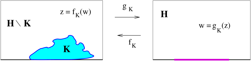
Figure 20: An example of hull $K$ in the upper hall plane together with the uniformizing map $f_{K}:\mathbb{H}\to\mathbb{H}\setminus\mathbb{K}$ and its invserse $g_{K}:\mathbb{H}\setminus\mathbb{K}\to\mathbb{H}$.

Consider for instance the hull formed by the segment $\{z=iy,\ y\in[0,a]\}$, $a>0$, drawn between the origin $0$ and point $ia$ in the upper half plane. The uniformizing map $g$ from $\mathbb{H}\setminus[0,ia]$ to $\mathbb{H}$ and its inverse are given by:

$$g(z)=\sqrt{z^{2}+a^{2}}\quad,\quad f(z)\equiv g^{-1}(z)=\sqrt{z^{2}-a^{2}}$$

The square root cut is specified by demanding that $g(z)\sim z$ at infinity so that $g(x)$ is negative (positive) on the real axis for $x$ negative (positive). It has a cut along the segment $[0,ia]$: the left hand of side of the segment is mapped on the real axis on the interval $[-a,0]$ and the right hand side on $[0,+a]$.

Another simple example is for $\mathbb{K}$ a semi-disc of radius $r$ centered on the origin $\{z\in\mathbb{H},\ |z|\leq r\}$. The uniformizing map of the upper half plane minus the semi-disc back onto the upper half plane is $g(z)=z+\frac{r^{2}}{z}$ and its inverse is $f(w)=\frac{1}{2}[w+\sqrt{w^{2}-4r^{2}}]$. It is clear that $g(z)$ is real for $z$ real or for $z$ on the semi-circle of radius $r$, so that the boundary of the upper half plane minus the semi-disc is mapped on the real axis.

A slight generalization consists in considering the infinitesimal hull $\mathbb{K}_{\epsilon;\rho}=\{z=x+i\epsilon y,\ 0<y\leq\pi\rho(x)\}$ made of the set of point included between the real axis and the curve $x\to i\epsilon\pi\rho(x)$, $\epsilon\ll 1$ with $x$ real. To first order in $\epsilon$, the normalized uniformizing map of $\mathbb{H}\setminus\mathbb{K}_{\epsilon;\rho}$ onto the upper half plane is

$$g(z)=z+\epsilon\int\frac{dx\rho(x)}{z-x}+\cdots,\quad\epsilon\ll 1,$$ (1)

as can be seen by covering the hull by a series of semi-disc, or by noticing that this map is real on the curve $z=x+i\epsilon\pi\rho(x)$.

Consider now again a domain $\mathbb{D}=\mathbb{H}\setminus\mathbb{K}$ with $\mathbb{K}$ generic hull and $f_{\mathbb{K}}$ its hydrodynamically normalized uniformizing map. As the boundary of $\mathbb{H}$ is smooth, $f_{\mathbb{K}}$ has a continuous extension to $\overline{\mathbb{R}}\equiv\mathbb{R}\cup\infty$, and $f_{\mathbb{K}}^{-1}(\overline{\mathbb{R}}\setminus\mathbb{K}_{\mathbb{R}})$ is a non-empty open set in $\overline{\mathbb{R}}$ with compact complement. We call the complement the cut of $f_{\mathbb{K}}$. By the Schwarz symmetry principle, defining $f_{\mathbb{K}}(z)=\overline{f_{\mathbb{K}}(\bar{z}})$ for $\Im{\rm m}\,z\leq 0$ gives an analytic extension of $f$ to the whole Riemann sphere minus the cut. Across the cut, $f$ has a purely imaginary non-negative discontinuity which we write as a Radon-Nikodym derivative $d\mu_{f_{\mathbb{K}}}/dx$. Cauchy’s theorem yields

$$f_{\mathbb{K}}(w)=w+\frac{1}{2\pi}\int_{\mathbb{R}}\frac{d\mu_{f_{\mathbb{K}}}(x)}{x-w},$$ (2)

Anticipating a little bit, let us note immediately that giving a dynamical rule for the evolution of the finite positive measure $d\mu_{f_{\mathbb{K}}}(x)$ is a good way to define growth processes. A quantity that plays an important role in the sequel is

$$C_{\mathbb{K}}\equiv\frac{1}{2\pi}\int_{\mathbb{R}}d\mu_{f_{\mathbb{K}}}(x),$$

a positive (unless $\mathbb{K}=\emptyset$) number called the capacity of $\mathbb{K}$, which is such that $f_{\mathbb{K}}(w)=w-C_{\mathbb{K}}/w+O(1/w^{2})$ at infinity. The usefulness of capacity stems from its good behavior under compositions: if $\mathbb{K}$ and $\mathbb{K}^{\prime}$ are two hulls, $\mathbb{K}\cup f_{\mathbb{K}}(\mathbb{K}^{\prime})$ is a hull and

$$C_{\mathbb{K}\cup f_{\mathbb{K}}(\mathbb{K}^{\prime})}=C_{\mathbb{K}}+C_{\mathbb{K}^{\prime}},$$ (3)

as seen by straightforward expansion at infinity of $f_{\mathbb{K}}\circ f_{\mathbb{K}^{\prime}}$, the map associated to $\mathbb{K}\cup f_{\mathbb{K}}(\mathbb{K}^{\prime}).$ In particular capacity is a continuous increasing function on hulls.

3.2 Evolutions

3.2.1 Loewner chains

Evolutions of family of increasing hulls $\mathbb{K}_{t}$ parameterized by some ‘time’ $t$ are going to be coded in the evolutions of their uniformizing map. Let $f_{t}\equiv f_{\mathbb{K}_{t}}$ be the conformal homeomorphism from $\mathbb{H}$ to $\mathbb{H}\setminus\mathbb{K}_{t}$ hydrodynamically normalized at infinity: $f_{t}(w)=w+O(1/w)$. Define $g_{t}:\mathbb{H}\setminus\mathbb{K}_{t}\mapsto\mathbb{H}$ to be the inverse of $f_{t}$. Then $g_{t}(z)=z+O(1/z)$ at infinity.

To study the evolution of the family of hulls $\mathbb{K}_{t}$, fix $\varepsilon\geq 0$ and consider the hull $\mathbb{K}_{\varepsilon,t}\equiv g_{t}(\mathbb{K}_{t+\varepsilon}\setminus\mathbb{K}_{t})$. Define $f_{\varepsilon,t}\equiv f_{\mathbb{K}_{\varepsilon,t}}$. Then $g_{t}=f_{\varepsilon,t}\circ g_{t+\varepsilon}$ on $\mathbb{H}\setminus\mathbb{K}_{t+\varepsilon}$. Using the representation of $f_{\mathbb{K}_{\varepsilon,t}}$ in terms of its discontinuity eq.(2), we obtain

$$g_{t+\varepsilon}(z)-f_{\varepsilon,t}\circ g_{t+\varepsilon}(z)=g_{t+\varepsilon}(z)-g_{t}(z)=\frac{1}{2\pi}\int_{\mathbb{R}}\frac{d\mu_{f_{\varepsilon,t}}(x)}{g_{t+\varepsilon}(z)-x}$$

For $\varepsilon$ small, the hull $\mathbb{K}_{\varepsilon,t}$ is small so that $f_{\varepsilon,t}$ is approaching the identity map and we may expect to be able to expand its discontinuity measure to first order in $\varepsilon$ as $d\mu_{f_{\varepsilon,t}}(x)\simeq\varepsilon 2\pi d\nu_{t}(x)$. In such cases, in the limit $\varepsilon\to 0$ we get the evolution equations:

$$\frac{d}{dt}g_{t}(z)=\int_{\mathbb{R}}\frac{d\nu_{t}(x)}{g_{t}(z)-x}$$ (4)

These sets of equations are called “Loewner chains”. The Loewner measures $d\nu_{t}$ may depend non linearly on the map $g_{t}$. They possess a simple physical interpretation. Indeed recall that the map $f_{\varepsilon,t}$ uniformizes $\mathbb{K}_{\varepsilon,t}$ which is the image by $g_{t}$ of the complement of $\mathbb{K}_{t}$ in $\mathbb{K}_{t+\varepsilon}$. The hull $\mathbb{K}_{\varepsilon,t}$ may be viewed as a domain bounded by the real axis and by a curve with height of order $\varepsilon$ and which is the image by $g_{t}$ of the matter added to go from $\mathbb{K}_{t}$ to $\mathbb{K}_{t+\varepsilon}$. The map $f_{\varepsilon,t}$ is then given by equation (1) to first order in $\varepsilon$ so that $d\nu_{t}(x)/dx$ is proportional to the height of the curve bounding $\mathbb{K}_{\varepsilon,t}$.

To make it more precise, let $f_{t}$, analytic in the upper half plane, be the inverse of $g_{t}$. It satisfies Loewner equation:

$$\frac{d}{dt}f_{t}(w)=-f^{\prime}_{t}(w)\,\int_{\mathbb{R}}\frac{d\nu_{t}(x)}{w-x}$$

This may be viewed as a Riemann-Hilbert problem for the ratio $\partial_{t}f_{t}(w)/f_{t}^{\prime}(w)$ since Loewner equation is equivalent to the following boundary value problem on the real axis:

$$\lim_{\varepsilon\to 0^{+}}\Im{\rm m}\,[\partial_{t}f_{t}(w)/f_{t}^{\prime}(w)]_{w=y+i\varepsilon}=\pi\rho_{t}(y)$$

with $d\nu_{t}(x)=\rho_{t}(x)dx$. By construction the boundary curve of the hull $\mathbb{K}_{t}$ is the image of the real axis, that is $f_{t}(\zeta)$, $\zeta\in\mathbb{R}$. Its evolution is governed by its normal velocity $v_{n}(\zeta)$ since the tangent velocity is parameterization dependent. The normal velocity is equal to $|f^{\prime}_{t}(\zeta)|\Im{\rm m}\,[\partial_{t}f_{t}/f_{t}^{\prime}](\zeta)$, so that it may be expressed in terms of the density $d\nu_{t}(x)$ as:

$$v_{n}(\zeta)\,d\zeta=\pi\,|f_{t}^{\prime}(\zeta)|\,d\nu_{t}(\zeta)$$

Comparing this formula with the previous heuristic interpretation with see that the factor $\varepsilon d\nu_{t}(\zeta)$ codes for the matter added in $\mathbb{K}_{\varepsilon,t}$ between time $t$ and $t+\varepsilon$ while $|f^{\prime}_{t}(\zeta)|$ is implementing the dilatation in going from $\mathbb{K}_{\varepsilon,t}$ to $\mathbb{K}_{t+\varepsilon}$.

Time parameterization has not yet been specified. In SLE context it is very useful – if not mandatory – to use the capacity as time variable so that we define the time parameter by $2t\equiv C_{\mathbb{K}_{t}}$. This imposes $\int_{\mathbb{R}}d\nu_{t}(x)=2$. The factor $2$ is just historical. The additivity property of capacity ensures the consistency of notation, namely $C_{\mathbb{K}_{t}\cup f_{\mathbb{K}_{t}}(\mathbb{K}_{s})}=t+s$. With this time parameterization, the maps behave as $g_{t}(z)=z+2t/z+O(1/z^{2})$ and $f_{t}(w)=w-2t/w+O(1/w^{2})$ at infinity.

3.2.2 Local growth

We introduce now the notion of local growth which is crucial for interfaces. In particular it applies to the case when the hulls $\mathbb{K}_{t}$ are portion of curves. Namely, let $\gamma_{[0,\infty]}$ be a simple curve from $0$ to $\infty$ in $\mathbb{H}$ and $\gamma_{]0,t]}$ be a portion of it with end point $\gamma_{t}$. Then $\mathbb{K}_{t}\equiv\gamma_{]0,t]}$ are growing hulls with capacity $2t$ by our choice of time parameterization. When $\varepsilon$ is small, $\mathbb{K}_{\varepsilon,t}\equiv g_{t}(\gamma_{]t,t+\varepsilon]})$ is a tiny piece of a curve and the support of the discontinuity measure $d\mu_{f_{\varepsilon,t}}$ is small and becomes a point when $\varepsilon$ goes to $0$. Measures supported at a point are $\delta$ functions, so there is a point $\xi_{t}$ such that, as a measure, $d\mu_{f_{\varepsilon,t}}/dx\sim 2\varepsilon\delta(x-\xi_{t})$ as $\varepsilon\rightarrow 0^{+}$. If $\mathbb{K}_{t}$ is a more general increasing family of hulls of capacity $2t$, we say that the condition of local growth is satisfied if the above small $\varepsilon$ behavior holds. At first sight, it might seem that local growth is only true for curves, but this is not true. We shall give an example below.

Letting $\varepsilon\rightarrow 0^{+}$, from the local growth condition, we infer the existence of a real function $\xi_{t}$ such that

$$\frac{dg_{t}}{dt}(z)=\frac{2}{g_{t}(z)-\xi_{t}}.$$ (5)

Had we used another parameterization of the curve, the $2$ in the numerator would be replaced by a positive function of the parameter along the curve.

It is useful to look at this equation from a slightly different point of view, taking the function $\xi_{t}$ as the primary data. For fixed $z$, this is a first order differential equation for $g_{t}$, which can be integrated at least for $t$ small enough. The solutions $g_{t}(z)$ of this equation for a given function $\xi_{t}$ with initial condition $g_{0}(z)=z$ is called a Loewner evolution. The image of $\xi_{t}$ by $g_{t}^{-1}$ is the tip $\gamma_{t}$ of the curve at time $t$. A more proper definition is

$$\gamma_{t}=\lim_{\epsilon\to 0^{+}}g^{-1}_{t}(\xi_{t}+i\epsilon)$$ (6)

In short $g_{t}(\gamma_{t})=\xi_{t}$. It is a theorem that if $\xi_{t}$ is regular enough – namely Hölder of exponent $>1/2$ – then $\gamma_{t}=g_{t}^{-1}(\xi_{t})$ is a curve. In particular continuity of $\xi_{t}$ is clearly a necessary condition for $\gamma_{t}$ to be a curve as otherwise any jumps in time of $\xi_{t}$ produce branchings in $\gamma_{t}$. The real function $\xi_{t}$ provides a parameterization of the growing curve $\gamma_{]0,\infty]}$.

Informally, if $\mathbb{K}_{t}$ is a growing curve, we expect that $g_{t+\varepsilon}(z)-g_{t}(z)$ describes an infinitesimal cut. This is confirmed by the explicit solution of eq.(5) for the trivial case $\xi_{t}\equiv 0$, which yields $g_{t}(z)^{2}=z^{2}+4t$, the branch to be chosen being such that at large $z$, $g_{t}(z)\sim z$. As previously explained, this describes a growing segment along the imaginary axis. So intuitively, the simple pole in eq.(5) accounts for the existence of a cut and different functions $\xi_{t}$ account for the different shapes of curves.

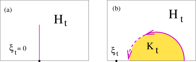
Figure 21: (a) The upper half plane cuted along a vertical slit. (b) The upper half plane cuted along a semi-circle. At the critical time at which the curve touches the real axis back, the hull is formed by all points surrounded by the curve, that is by the semi-disc.

One can also solve the case when $\mathbb{K}_{t}$ is an arc of circle going from $0$ to $2R$ along a circle of radius $R$. In this case the driving function is $\xi_{t}=3[R-\sqrt{R^{2}-2t}]$. See Fig.21. It has a square root singularity $\xi_{t}\propto\sqrt{R^{2}-2t}$ when the arc approaches the real axis at time $t_{c}=R^{2}/2$. The capacity remains finite, and goes to $R^{2}$, and the map itself has a limit $g_{t_{c}}(z)=z+R^{2}/(z+R)$ which has swallowed the half disk without violating the local growth condition. One can start the growth process again. Making strings of such maps with various values of the radii is a simple way to construct growing families of hulls that are not curves and that nevertheless grow locally. Note that a square root singularity for $\xi_{t}$ is the marginal behavior as if $\xi_{t}$ is Hölder of exponent $>1/2$, Loewner evolution yields a simple curve.

3.3 Miscellaneous iterations

Uniformizing maps are defined up to $SL(2,\mathbb{R})$ transformations and so do the Loewner equations. These equations also take different forms depending on which domain is used as a reference domain. Above we chose the upper half plane as reference domain and the hydrodynamic normalization to fix the uniformizing map uniquely. It leads to eq.(4) which is usually called chordal Loewner evolutions. There are other possibilities and some of them will be discussed below in connection with different SLE configurations.

In Section 8.1, we shall present another version of Loewner equation, called radial Loewner evolution, which uses the unit disk as a reference domain. The conformal map are then uniquely fixed by imposing normalization conditions on a bulk point.

There is yet another way to generalize the previous evolutions. It consists in discretizing the time parameter so that the evolutions are then defined by successive iterations of conformal maps. The elementary maps involved at each iteration code for the addition of tiny pieces to the domain. This procedure will be described in Section 8.4.

4 Stochastic Schramm-Loewner evolution

We are interested in the continuous limit of the interfaces of 2d statistical we just described in Section 2 at criticality. Based on heuristic arguments of scale invariance plus locality, it was conjectured in [21] about twenty years ago that such curves should be conformally invariant (in an appropriate sense). This statement was made really precise and powerful by Oded Schramm who understood what are the consequences of conformal invariance for a set of random curves and how to exploit them. This leads him to the definition of the Loewner-Schramm stochastic evolutions (SLE).

The aim of this Section is to explain Schramm’s argument in the simplest case, called chordal SLE, describing curves joining two boundary points of a planar domain.

Let us fix the notation.

Consider a domain $\mathbb{D}$, with two distinct points on its boundary, which we call $a$ and $b$. A simple curve, denoted by $\gamma_{[ab]}$, from $a$ to $b$ in $\mathbb{D}$ is the image of a continuous one-to-one map $\gamma$ from the interval $[0,+\infty]$ to $\mathbb{D}\cup\{a,b\}$ such that $\gamma(0)=a$, $\gamma(\infty)=b$ and $\gamma_{]ab[}\equiv\gamma(]0,\infty[)\subset\mathbb{D}$. Alternatively, a simple curve from $a$ to $b$ is an equivalence class of such maps under increasing reparametrizations. A point on it has no preferred coordinate but is has a past and a future. If $c\in\mathbb{D}$ is an interior point, we use a similar definition for a simple curve $\gamma_{[ac]}$ from $a$ to $c$ in $\mathbb{D}$.

For any of these, we use ${\bf P}_{(\mathbb{D},a,b)}$ to denote the probability distribution for the interface $\gamma_{[ab]}$ from $a$ to $b$ in $\mathbb{D}$.

4.1 Conformal covariance

Before embarking into Schramm’s argument let us point out a possible caveat concerning conformal invariance. If a probability measure on curves, or hulls, is defined say in the upper half plane $\mathbb{H}$, one can always transport it to any other non empty simply connected open sets in $\mathbb{C}$ to get new probability measures on curves or hulls. But if we have nothing against which to compare the transported measures, this statement is purely tautological – and almost empty – since it just tells us how to transport probability measures. What is highly nontrivial is that continuum limits of discrete 2D critical statistical mechanics models are conformally covariant. Such models are usually defined on a lattice, say $a\mathbb{Z}+ia\mathbb{Z}$ where $a>0$ is a unit of length. Criticality is the statement that when $a$ goes to zero certain nontrivial physical observables survive and do not depend on any scale. The limit has to be defined carefully. If $\mathbb{U}$ and $\mathbb{V}$ are two conformally equivalent open subsets of $\mathbb{C}$, related by a conformal map $\varphi$, one can consider the model in the intersection of the lattice $a\mathbb{Z}+ia\mathbb{Z}$ with $\mathbb{U}$ or $\mathbb{V}$. When $a$ goes to $0$, scale invariance does not a priori imply that the limit theories on $\mathbb{U}$ and $\mathbb{V}$ are related in a simple way. Using another physical language, it was conjectured in [21] that the limiting theory is well defined on the abstract Riemann surface which is the equivalence class of all open subsets of $\mathbb{C}$ conformally equivalent to $\mathbb{U}$. For instance correlation functions of local observables become sections of appropriate bundles, i.e. have transformations that involve derivatives of $\varphi$ when going from $\mathbb{U}$ to $\mathbb{V}$. Interfaces are directly related by $\varphi$ and the probability law governing their fluctuations as well.

As we shall explain, SLE curves behave geometrically as they should to encode the statistics of critical interfaces. They have the proper behavior under conditioning and conformal transformations. However, they do it in a very specific way, involving Loewner evolutions and $1d$ Brownian motion. Schramm’s argument for SLE may be decomposed in three steps:
(i) a comparison of the probability distribution of curves $\gamma_{[ab]}$ in a domain $\mathbb{D}$ conditioned on a portion $\gamma_{[ac]}$ of the curve with the probability distribution in the cutted domain $\mathbb{D}\setminus\gamma_{[ac]}$;
(ii) a formulation of conformal transport of probability distributions of curves between two conformally equivalent domains;
(iii) a mixture of the two previous steps which implies a Markov and stationarity of increments property for conformally invariant random curves.
Let us make it plain.

4.1.1 The domain Markov property

We first go to the point, valid for all the discrete examples we have described, which relates properties of conditioned probability of curves to properties of models of statistical mechanics.

Suppose that we fix the beginning $\gamma_{[ac]}$ of a possible interface in domain $\mathbb{D}$, up to a certain point $c$. Then:
(i) we can consider the conditional distribution for the rest of the interface and
(ii) we can remove the beginning of the interface from the domain to create a new domain and consider the distribution of the interface in this new domain.
This is illustrated on Fig.18 on the lattice and in Fig.27 on the continuum.

We claim – or demand – that the distributions defined in (i) and (ii) coincide, ie.:

$$\gamma_{[ab]}\ {\rm in}\ \mathbb{D}\ |\ \gamma_{[ac]}\equiv_{{\rm in~{}law}}\gamma_{[cb]}\ {\rm in}\ \mathbb{D}\setminus\gamma_{[ac]}$$

where the vertical line means ‘conditioned by’. Equivalently, in equations:

$${\bf P}_{(\mathbb{D},a,b)}[\;.\;|\gamma_{[ac]}]={\bf P}_{(\mathbb{D}\setminus\gamma_{[ac[},c,b)}[\;.\;].$$ (7)

It is obvious that these two probabilities are supported on the same set, namely simple curves along the edges of the lattice, going from $c$ to $b$ in $\mathbb{D}\setminus\gamma_{[ac[}$.

In the lattice statistical mechanics formulation, this property is a simple consequence for instance of the locality of the interaction. Let us however note that for loop-erased random walks, annihilating boundary conditions are crucial. Reflecting boundary conditions clearly do not work, if only because the supports do not coincide in that case.

For the case of percolation and the Ising model, in fact more is true: we can view ${\bf P}_{(\mathbb{D},a,b)}$ not only as a probability distribution for the interface, but as the full probability distribution for the colors of the hexagons and still check the identity of (i) and (ii). Again, the supports are the same for (i) and (ii), namely any configuration of the colors, except that the colors on both sides of $\gamma_{[ac]}$ are fixed. For the case of percolation, the colors are independent of each other so the identity of (i) and (ii) is clear. For the Ising model, the difference is that the conditional probabilities in (i) take into account the interactions between the colors along the interface, whereas the probability in (ii) does not take into account the interactions between the spins along the cut left by the removal of the interface. However, as already mentioned above, the corresponding colors are fixed anyway, so the Boltzmann weights for the configurations that are in the support of (i) or (ii) differ by a multiplicative constant, which disappears when probabilities are computed.

This argument extends immediately to systems with only nearest neighbor interactions. They can be defined on any graph. If any subset of edges is chosen and the configuration at both end of each edge is frozen, it makes no difference for probabilities to consider the model on a new graph in which the frozen edges have been deleted. Instead of looking for further generalizations, we argue more heuristically that the continuum limit for a system with short range interactions should satisfy locality property. Its use – which, as should be amply evident, has nothing to do with conformal invariance – together with the conformal invariance assumption is at the heart of O. Schramm’s derivation of stochastic Loewner evolutions.

4.1.2 Conformal transport

For studying conformally invariant probability measures on the set of simple curves from $a$ to $b$ in $\mathbb{D}$, there is a purely kinematic step which demands that if $h$ is any conformal map that sends $\mathbb{D}$ to another domain $\hat{\mathbb{D}}\equiv h(\mathbb{D})$, the measure for $(h(\mathbb{D}),h(a),h(b))$ should be the image by $h$ of the measure for $(\mathbb{D},a,b)$. Namely:

$$h(\gamma_{[ab]}\ {\rm in}\ \mathbb{D})\equiv_{{\rm in~{}law}}\gamma_{[h(a)h(b)]}\ {\rm in}\ h(\mathbb{D})$$

or explicitly,

$${\bf P}_{(\mathbb{D},a,b)}[\gamma_{[ab]}\subset U]={\bf P}_{(h(\mathbb{D}),h(a),h(b))}[\gamma_{[h(a)h(b)]}\subset h(U)],$$

where ${\bf P}_{(\mathbb{D},a,b)}[\gamma_{[ab]}\subset U]$ denotes the probability for the curve $\gamma_{[ab]}$ to remain in a subset $U$ of $\mathbb{D}$. See Fig.22.

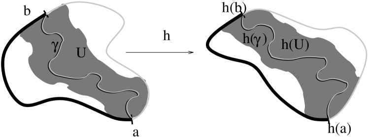
Figure 22: Conformal invariance for change of domain. The measure on curves is simply transported by the conformal map.

This condition is natural and it is the one that conformal field theory suggests immediately. Let us note however that a totally different definition of conformal invariance is understood in the familiar statement “two dimensional Brownian motion is conformally invariant”.

Without any further constraint this condition is a kind of tautology as it only tells how to transport the measure from one domain to another. It only imposes to the measure to be invariant under the one parameter group of automorphisms that fixes $(\mathbb{D},a,b)$. Indeed we could take any measure for $(\mathbb{D},a,b)$ – well, with the invariance under the one parameter group of automorphisms that fixes $(\mathbb{D},a,b)$ – and declare that the measure in $h(\mathbb{D})$ is obtained by definition by the rule above.

This condition becomes a non empty statement only when we start comparing the transported measures with those obtained as continuum limits of measures of discrete interfaces of lattice statistical models. If this condition holds for the limit measure the interfaces are said to be conformally invariant.

To make progress – without going back to the discrete models – we need to combine conformal invariance with the domain Markov property. This is the basic observation made by O. Schramm.

4.1.3 Conformally invariant interfaces

This short Section establishes the most crucial properties of conformally invariant interfaces: the Markov property and the stationarity of increments of conformally invariant interfaces.

Take $c\in\mathbb{D}$ and let $\gamma_{[ac]}$ be a simple curve from $a$ to $c$ in $\mathbb{D}$. Observe that $\mathbb{D}\setminus\gamma_{]ac]}$ is a domain. To answer the question “if the beginning of the interface is fixed to be $\gamma_{[ac]}$, what is the distribution of the rest $\gamma^{\prime}_{[cb]}$ of the interface?” we apply the domain Markov property to argue that this is exactly the distribution of the interface in $\mathbb{D}\setminus\gamma_{]ac]}$. We map this domain conformally to $\mathbb{D}$ via a map $h_{\gamma_{[ac]}}$ sending $b$ to $b$ and $c$ to $a$:

$$h_{\gamma_{[ac]}}(\mathbb{D}\setminus\gamma_{]ac]})=\mathbb{D}\quad h_{\gamma_{[ac]}}(c)=a\quad h_{\gamma_{[ac]}}(b)=b$$

so that the image by $h_{\gamma_{[ac]}}$ of the rest of the curve $\gamma^{\prime}_{[cb]}$ is curve from $a$ to $b$ in $\mathbb{D}$, see Fig.23.

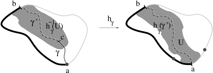
Figure 23: Conformal invariance for conditional probabilities.

Conformal transport implies that the image measure is the original measure, ${\bf P}_{(\mathbb{D},a,b)}[\cdot|\gamma_{[ac]}]=h_{\gamma_{[ac]}}^{*}\circ{\bf P}_{(\mathbb{D},a,b)}[\cdot]$, so that $h_{\gamma_{[ac]}}(\gamma^{\prime}_{[cb]})$ behaves an interface from $a$ to $b$ that has forgotten $\gamma_{[ac]}$. More explicitly:

$${\bf P}_{(\mathbb{D},a,b)}[\gamma_{[cb]}\subset U|\gamma_{[ac]}]={\bf P}_{(\mathbb{D},a,b)}[\gamma_{[ab]}\subset h_{\gamma_{[ac]}}(U)],$$

for any subset $U\subset\mathbb{D}\setminus\gamma_{]ac]}$.
To summarize :

$h_{\gamma_{[ac]}}(\gamma^{\prime}_{[cb]})$ is independent of $\gamma_{[ac]}$ (the Markov property) and has the same distribution as the original interface itself from $a$ to $b$ (stationarity of increments).

This property is what is meant by conformallly invariant interfaces and is the main observation done by Schramm [118].

We end this Section with another caveat. The above statement, that SLE is conformally covariant under domain changes, should not be confused with the, incorrect in general, statement that SLE growth processes are conformally invariant in the sense 2d Brownian motion is conformally invariant. A local conformal transformation maps Brownian motion to Brownian motion modulo a random time change. But SLE is conformally invariant in that sense only in a special case, namely for $\kappa=6$ which corresponds to percolation for which the central charge and the conformal weight to be introduced later both vanish. See Section 5.3.

4.2 Chordal SLE: basics

The Markov and stationarity of increments property make it plain that to understand the distribution of the full interface, it is enough to understand the distribution of a small, or even infinitesimal, initial segment, and then glue segments via conformal maps.

This calls for a description by differential equations, which turns out to be conveniently described by Loewner evolutions.

For clarity let us recall basics and notations from Section 3. Using conformal invariance, we can restrict ourselves to the situation when $(\mathbb{D},a,b)=(\mathbb{H},0,\infty)$. If $\gamma_{[0\infty]}$ is a simple curve from $0$ to $\infty$ in $\mathbb{H}$, and $\gamma_{t}$ a point on it, we know that $\mathbb{H}\setminus\gamma_{]0,t]}$ is a domain. As in previous Section, it is convenient to use the capacity as a parameterization and define a time parameter by $2t\equiv C_{\gamma_{]0,t]}}$.

Let $f_{t}$ be the conformal homeomorphism from $\mathbb{H}$ to $\mathbb{H}\setminus\gamma_{]0,t]}$ normalized to satisfy $f_{t}(w)=w-2t/w+O(1/w^{2})$ at infinity. Define $g_{t}:\mathbb{H}\setminus\gamma_{]0,t]}\mapsto\mathbb{H}$ to be the inverse of $f_{t}$. It satisfies $g_{t}(z)=z+2t/z+O(1/z^{2})$ at infinity. Then, for $\gamma_{]0,t]}$ a simple curve, there exists a real function $\xi_{t}$ such that the time evolution of these maps – and therefore the growth of the curve – are described by the first order Loewner differential equation (5):

$$dg_{t}(z)/dt=2/(g_{t}(z)-\xi_{t}).$$

The solutions of this equation for a given function $\xi_{t}$ with initial condition $g_{0}(z)=z$ is called a Loewner evolution. By construction, the image of $\xi_{t}$ by $g_{t}^{-1}$ is the tip of the curve at time $t$, $\gamma_{t}=\lim_{\varepsilon\to 0^{+}}g_{t}^{-1}(\xi_{t}+i\varepsilon)$, so that the function $\xi_{t}$ provides an alternative parameterization of the curve.

More generally, see Section 3, if $\xi_{t}$ is not regular enough – eg. if it has square root singularity – solutions of the Loewner equation (5) may produce conformal maps $g_{t}$ which uniformize the complements of hulls $\mathbb{K}_{t}\equiv\mathbb{H}\setminus g_{t}^{-1}(\mathbb{H})$ which do not coincide with the curves $\gamma_{]0,t]}$ but which are grown locally from these curves.

With these tools in hands we may now conclude Schramm’s argument and present the definition of SLEs.

4.2.1 Definition

If we sample locally growing hulls $\mathbb{K}_{t}$ with a certain distribution, we get an associated random process $\xi_{t}$. In the case of a conformally invariant distribution, we have established two crucial properties: Markov property and stationarity of increments. To finish Schramm’s argument leading to SLE, what remains is to see the implications of these properties on the distribution of $\xi_{t}$.

The argument and expressions for the meaning of Markov property and stationarity of increments involved a map $h$ that mapped the tip of the piece of interface to the initial marked point $a$ and the final marked point $b$ to itself. The map $h_{t}(z)=g_{t}(z)-\xi_{t}$ has the required property when the domain is the upper-half plane with $0$ and $\infty$ as marked points: it maps the tip of the curve back to the origin. It behaves like $h_{t}(z)=z-\xi_{t}+2t/z+O(1/z^{2})$ at infinity. We infer that for $s>t$, $h_{t}(\mathbb{K}_{s}\setminus\mathbb{K}_{t})$ is independent of $\mathbb{K}_{t^{\prime}},\;t^{\prime}\leq t$ (Markov property) and is distributed like a hull of capacity $s-t=C_{h_{t}(\mathbb{K}_{s}\setminus\mathbb{K}_{t})}$ (stationarity of increments).

The hull determines the corresponding map $h$, so this can be rephrased as: the map $h_{s}\circ h_{t}^{-1}$, which uniformizes $h_{t}(\mathbb{K}_{s}\setminus\mathbb{K}_{t})$, is independent of $h_{t^{\prime}},\;t^{\prime}\leq t,$ and distributed like an $h_{s-t}$. As $h_{s}\circ h_{t}^{-1}=z-(\xi_{s}-\xi_{t})+2(s-t)/z+O(1/z^{2})$ at infinity, the driving parameter for the process $h_{s}\circ h_{t}^{-1}$ is $\xi_{s}-\xi_{t}$. To summarize:

the Markov property and stationarity of increments for the interface lead to the familiar statement for the process $\xi_{t}$: for $s>t$, $\xi_{s}-\xi_{t}$ is independent of $\xi_{t^{\prime}},\;t^{\prime}\leq t,$ (Markov property) and distributed like a $\xi_{s-t}$ (stationarity of increments).

To conclude, two last physical inputs are needed. One first demands that the interface does not branch, which means that at two nearby times the growth is at nearby points. This implies that $\xi_{t}$ is a continuous process, in the sense that it has continuous trajectories. One also requires that the distribution of the curve is left-right symmetric under reflexion with to respect to the imaginary axis. This implies that $g_{t}(z)$ and $-\overline{g_{t}(-\bar{z})}$ are identically distributed which as consequence implies that $\xi_{t}$ and $-\xi_{t}$ are alike.

One is now in position to apply a mathematical theorem: a 1d Markov process with continuous trajectories, stationary increments and reflexion symmetry is proportional to a Brownian motion. We conclude that there is a real positive number $\kappa$ such that $\xi_{t}=\sqrt{\kappa}B_{t}$ for some normalized Brownian motion $B_{t}$ with covariance $\mathbb{E}[B_{s}B_{t}]=\min(s,t)$. The same argument without imposing that the time parameterization is given by the capacity of the hull would lead to the conclusion that the driving parameter is a continuous martingale, which is nothing but a Brownian motion after a possibly random time change.

To summarize:
A solution of Loewner equation with a Brownian motion as driving term,

$$\frac{dg_{t}}{dt}(z)=\frac{2}{g_{t}(z)-\xi_{t}}\quad,\quad\xi_{t}=\sqrt{\kappa}B_{t},$$ (8)

with $g_{t=0}(z)=z$, is called a chordal Schramm-Loewner evolution of parameter $\kappa$, in short a chordal SLE, in the upper half plane $\mathbb{H}$ with two marked points $0$ and $\infty$. Given $z\in\mathbb{H}$, eq.(8) may be integrated up to time $\tau_{z}$, called the swallowing or exploding time, for which $g_{\tau_{z}}(z)=\xi_{\tau_{z}}$.

By construction, chordal SLE enjoys the two following properties:

• $g_{t}(z)$ and $g_{\lambda^{2}t}(\lambda z)$ are identically distributed. This is direct consequence of usual scaling property of the Brownian motion. Since dilatation is the only conformal map preserving the upper half plane with its two marked points $0$ and $\infty$, this ensures the coherence of the process.

• $h_{t}(z)\equiv g_{t}(z)-\xi_{t}$ has the Markov property. Furthermore, $h_{s}\circ h_{t}^{-1}$ is independent of $h_{t}$ and distributed as $h_{s-t}$ for $s>t$. Again this is a direct consequence of Brownian motion properties.

The connection of this equation with interfaces relies mainly on conformal invariance. But local growth, absence of branches, and to a lower level locality at the interface, also play a crucial role.

4.2.2 Basics properties

The set of exact results obtained for SLE forms an impressive body of knowledge. See for instance the physical [67, 74, 12, 34] or mathematical [101, 134, 138] reviews. In this Section, we list just a few “pictorial” properties with some comments and we leave more detailed computations for the following Sections. They – the properties and the comments – should be understood with the standard proviso “almost surely” or “with probability $1$”.

We start with a surprisingly difficult result [118, 90, 91, 92, 115, 20].

• Whatever the value of $\kappa$, the pre-image of the driving parameter

  $$\gamma_{t}\equiv\lim_{\varepsilon\rightarrow 0^{+}}g_{t}^{-1}(\sqrt{\kappa}B_{t}+i\varepsilon)$$

  is a continuous curve, called the SLE trace. The curve starts at $\xi_{t=0}=0$ and it reaches the point at infinity at infinite time, $\lim_{t\to\infty}\gamma_{t}=\infty$. The trace never crosses itself. This property is crucial if the trace is to be interpreted as a curve separating two phases.

• For $\kappa\in[0,4]$ the SLE trace is a simple curve. For $\kappa\in]4,8[$, it has double points. For $\kappa\in[8,\infty[$, it is space filling. A probabilistic argument for this property is given at the end of this Section.

• The fractal dimension $d_{\kappa}$ of the trace is $1+\kappa/8$ for $\kappa\leq 8$ and $2$ for $\kappa\geq 8$. See Section 7.4.

Using the formula for the dimension of the trace and confronting with the numerical simulations of Section 2, it is plausible (actually, these are among the few cases for which a mathematical proof exists) that loop-erased random walks correspond to $\kappa=2,d=5/4$ and percolation to $\kappa=6,d=7/4$. This is also compatible with the general shape of the numerical samples, which indicate that loop-erased random walks indeed lead to simple curves and that percolation doesn’t.

The hull $\mathbb{K}_{t}$ is by definition $\mathbb{H}\setminus g_{t}^{-1}(\mathbb{H})$. It is also the set of point which have been swallowed by the trace at time $t$, namely $\mathbb{K}_{t}=\{z\in\mathbb{H};\ \tau_{z}<t\}$. It has the following properties:

• The hull $\mathbb{K}_{t}$ is the complement of the connected component of $\infty$ in $\mathbb{H}\setminus\gamma_{]0,t]}$.

• For $\kappa\in[0,4]$, the SLE hull is a simple curve coinciding with the trace. For $\kappa\in]4,\infty[$, the SLE hull has a non empty connected and relatively dense interior.

Furthermore, there is a duality conjecture which states that the exterior frontiers of SLE hulls for $\kappa>4$ looks locally as SLE curves but for a dual value $\kappa_{*}=16/\kappa<4$. It is still unproved.

These properties may seem surprising at first sight. They are the signs that for $\kappa>4$, the drift $\sqrt{\kappa}B_{t}$ goes fast enough for the swallowing procedure to take place, as described in the previous closing arc example, but on all scales. Although, for $4<\kappa<8$, SLE produces non trivial hulls $\mathbb{K}_{t}$, the tip of the curves $\gamma_{[0,t]}$ is always emerging from the hulls towards infinity and never reenter into the hull. This is a consequence of local growth. This is summarized by Fig.24.

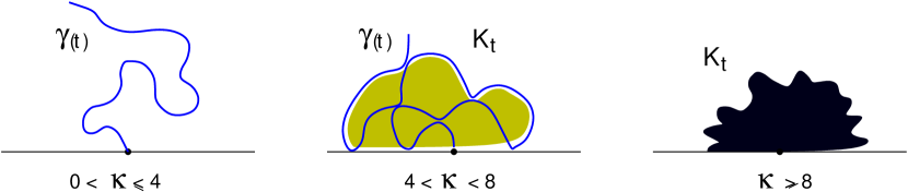
Figure 24: The phases of SLE.

The existence of these different phases may be grasped by looking at the motion of a point of the real axis. So let $x\in\mathbb{R}$ and consider the real process $Y_{t}\equiv h_{t}(x)/\sqrt{\kappa}=(g_{t}(x)-\xi_{t})/\sqrt{\kappa}$. By construction it is a Bessel process since it satisfies the stochastic equation $dY_{t}=\frac{(2/\kappa)}{Y_{t}}dt+dB_{t}$. A $d$-dimensional Bessel process is the process given by the modulus of Brownian motion in dimension $d$. If $R_{t}$ denotes this modulus, it satisfies the stochastic equation $dR_{t}=\frac{(d-1)/2}{R_{t}}+dB_{t}$, see Appendix A. So the effective dimension for the process $Y_{t}$ is $d_{\rm eff}=\frac{4+\kappa}{\kappa}$. Now a Brownian motion is recurrent in dimension less than $2$ – meaning that it reaches the origin an infinite number of times with probability one – and not recurrent in dimension bigger than $2$. So with probability one $Y_{t}$ vanishes in finite time with probability one for $\kappa>4$ and remains finite with probability one for $\kappa<4$. Since the vanishing of $Y_{t}$ signals that the SLE curve has touched the real axis between $x$ and $\infty$, this tells us that the SLE curve touches the real axis an infinite number of time with probability one for $\kappa>4$ and does not touch the real axis for $\kappa<4$. Markov and independent increment properties then imply that the curve has an infinite number of double points for $\kappa>4$ and none for $\kappa<4$. We shall present in a following Section an argument indicating the SLE trace is space filling for $\kappa>8$. The phase diagram simply expresses this behavior.

Nice images of SLE and other growth processes can be found on Vincent Beffara’s webpage http://www.umpa.ens-lyon.fr/ṽbeffara/pics.php. We just quote two examples, $\kappa=4$ and $\kappa=6$ on Fig.25.

      

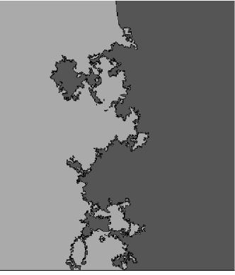
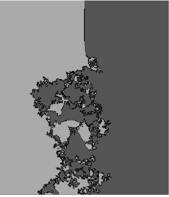
Figure 25: Two SLE samples for $\kappa=4$ and $\kappa=6$.

4.3 Other SLEs

Chordal SLEs yield measures $P_{(\mathbb{D},a,b)}$ on sets of curves joining two boundary points $a$, $b$ of a domain $\mathbb{D}$. There are a few other versions of SLEs corresponding to different boundary conditions. In simply connected planar domains, there are three possible definitions (preserving reflection symmetry): chordal, radial and dipolar SLEs. A group theoretical explanation of this classification will be given in the following Section 4.4. As for chordal SLE, they are defined via a version of Loewner equation for a uniformizing map $g_{t}$ from which one reconstructs the curve. They are conformally invariant in the sense that they satisfy the Markov and identical increment properties. They differ by their global topological behavior but their local properties are identical. For instance, they have three different phases depending on the value of $\kappa$ as for chordal SLE – with the same phase diagram – and their traces have identical fractal dimensions.

There has been attempts to specify SLE in two dimensional manifold of more general topology. See Section 5.6 for an overview. Here we shall only present the definition of SLEs in simply connected domains. For each SLE there is an adapted geometry – the upper half plane was adapted to chordal SLE – and we shall use these geometries to give the definitions but, of course, the processes can be defined in any geometry by conformal transport.

4.3.1 Radial SLE

Radial SLE [118, 115, 90, 101] describes curves joining a point on the boundary to a point in the bulk of the domain, which have to be specified. So the radial SLE data are: the domain $\mathbb{D}$, the starting boundary point $x_{0}$ and the final bulk point $z_{*}$. Notice that there is no non-trivial global conformal transformation preserving these data (contrary to the chordal case in the upper half plane in which dilatation preserves the data). It was originally defined using the unit disk as reference domain $\mathbb{D}=\{z,\ |z|<1\}$ with $1$ as the boundary point where the SLE trace emerges and $0$ as the inside point where the SLE trace converges. The Loewner equation then becomes:

$$\partial_{t}g_{t}(z)=-g_{t}(z)\ \frac{g_{t}(z)+U_{t}}{g_{t}(z)-U_{t}},\quad U_{t}=\exp(i\xi_{t})$$ (9)

with $g_{t=0}(z)=z$. The origin is kept fix $g_{t}$ and the map is normalized so that its derivative at the origin is real. The time $t$ is defined via $g_{t}^{\prime}(0)=e^{t}$. The radial SLE trace $\gamma_{t}$ is reconstructed via the Loewner map by $\gamma_{t}=g_{t}^{-1}(U_{t})$. As for chordal SLE, the hull coincides with the trace for $0<\kappa\leq 4$ and the curve has infinitely many double points for $4\leq\kappa\leq 8$.

Radial SLE is particularly simple on a semi-infinite cylinder of circumference $\Lambda\pi$, whose boundary is a circle. In this geometry the defining equation simply reads:

$$\frac{dg_{t}}{dt}(z)=\frac{2\Lambda^{-1}}{\tan[(g_{t}(z)-\xi_{t})/\Lambda]},\quad\xi_{t}=\sqrt{\kappa}B_{t}$$ (10)

The trace $\gamma_{t}=g^{-1}(\xi_{t})$ starts on the boundary of the cylinder and winds many times before reaching infinity, which is a bulk point of the cylinder.

Without breaking conformal invariance, ie. the Markov and independent increment property, we have the freedom in radial SLE to choose as driving source $U_{t}=\sqrt{\kappa}B_{t}+\alpha t$, with a linear-in-time drift term, instead of the simple choice $\xi_{t}=\sqrt{\kappa}B_{t}$. In the disc geometry, this breaks rotation invariance but provides a way to account for the winding number of the SLE trace around the origin.

4.3.2 Dipolar SLE

To define dipolar SLE [13] one specifies a boundary point, which is going to be the starting point of the trace, and a boundary interval not including the starting point, which is going to included the termination point of the trace. Then dipolar SLE describes curves starting on the specified boundary point and stopped the first instant they hit the specified boundary interval. So the dipolar SLE data are: the domain $\mathbb{D}$, the starting point $x_{0}$ and the two boundary points $x_{\pm}$ of the terminal interval $[x_{-},x_{+}]$. As for radial SLE, there is no non-trivial conformal map preserving this data. An adapted geometry is the strip of width $\pi\Delta$, $\mathbb{S}_{\Delta}=\{z,\ 0<\Im{\rm m}z<\pi\Delta\}$, with two boundary points at $\pm\infty$, in which case the equation reads:

$$\frac{dg_{t}}{dt}(z)=\frac{\Delta^{-1}}{\tanh[(g_{t}(z)-\xi_{t})/2\Delta]},\quad\xi_{t}=\sqrt{\kappa}B_{t}$$ (11)

with $g_{t=0}(z)=z$. The trace $\gamma_{t}=g^{-1}(\xi_{t})$ starts at the origin and ends randomly on the upper boundary side. For $0<\kappa\leq 4$, the hull coincide with the trace which is then a curve joining lower and upper boundary side, touching them only once. For $4\leq\kappa\leq 8$, the curve has infinitely many double points so that it does not coincide with its hull. The hulls touch the lower boundary infinite many times but only once the upper boundary – and this happens at infinite time. As a consequence the hulls do not invade the full domain but only a random subset of it, and this is one of the main differences between dipolar SLE and chordal or radial SLE.

In the limit of infinitely large strip dipolar SLEs converge to chordal SLEs on the upper half plane or, alternatively, chordal SLEs describe locally dipolar SLEs in the neighborhood of their starting points. This indirectly shows that the chordal SLE traces reach the point at infinity with probability one.

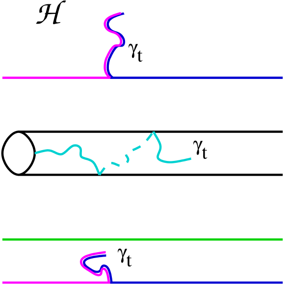
Figure 26: Three avatars of SLE: chordal, radial and dipolar.

4.3.3 SLE($\kappa,\rho$)

SLE($\kappa,\rho$) involves [97] the same data as dipolar SLE: the domain $\mathbb{D}$, the starting point $x_{0}$ and two other boundary points $x_{+}$ and $x_{-}$. Although not originally defined this way, it may be viewed as a generalization of dipolar SLE in which reflection symmetry is not imposed but conformal invariance is still preserved. This is possible because there is no non-trivial global conformal map preserving the data. In the strip geometry of width $\Delta\pi$, with the boundary points $x_{\pm}=\pm\infty$, this amounts to add a linear-in-time drift to the driving term, so that the defining equation becomes:

$$\frac{dg_{t}}{dt}(z)=\frac{\Delta^{-1}}{\tanh[(g_{t}(z)-U_{t})/2\Delta]},\quad U_{t}=\sqrt{\kappa}B_{t}+\alpha t$$ (12)

with $g_{t=0}(z)=z$. The effect of the drift is to push the SLE trace preferably towards one of the two boundary points $x_{\pm}$. Of course it reduces to dipolar SLE for $\alpha=0$.

SLE($\kappa,\rho$) were initially defined in the upper half plane $\mathbb{H}$, with a marked point $x$ on the real line, via the stochastic equation:

$$d\hat{g}_{t}(z) = \frac{2dt}{\hat{g}_{t}(z)-\hat{U}_{t}},$$ (13)

$$d\hat{U}_{t} = \sqrt{\kappa}dB_{t}+\frac{\rho\,dt}{\hat{U}_{t}-\hat{g}_{t}(x)}$$

The trace emerges from the point $\hat{U}_{0}$, say $x<\hat{U}_{0}$, and ends on the real axis between point $x$ and the point at infinity. For $\rho=0$ it reduces to SLE_κ and SLE($\kappa,\kappa-6$) is a chordal SLE from $U_{0}$ to $x$ but with a non standard normalization of the conformal map.

The two descriptions are actually equivalent, as shown for instance in [84, 121]. The mapping from one definition to the other requires mapping conformally the strip into the upper half plane, with the appropriate normalization, and a random time change. The definition via eqs.(13) treats the two marked points $x$ and $\infty$ very asymmetrically contrary the first definition (12). The relation between $\alpha$ and $\rho$ is $\rho=\frac{\kappa-6}{2}+\alpha$. In particular, SLE($\kappa,\frac{\kappa-6}{2}$) is equivalent to dipolar SLE.

To make explicit the relation between the two descriptions is computationally a bit long so we only give hints for it. We start from the first formulation in a strip of width $\pi$ and define $k_{t}(z)=\exp(-t+g_{t}(\log z))$ and $W_{t}=\exp(-t+U_{t})$. The map $k_{t}$ is, up to a random time change and a translation, the SLE$(\kappa,\rho)$ map in the upper half plane with marked point $x=0$ and starting point $\hat{U}_{0}=1$. So let us change time by defining $ds=W^{2}_{t}dt$ and $Z_{s}=W_{t(s)}$. We set $\hat{g}_{s}(z)=k_{t(s)}(z)+X_{s}$ and $\hat{U}_{s}=Z_{s}+X_{s}$ with $X_{s}$ solution $dX_{s}=-\frac{2ds}{Z_{s}}$. Then $\hat{g}_{s}$ and $\hat{U}_{s}$ satisfy the SLE$(\kappa,\rho)$ equation (13) with $X_{s}=\hat{g}_{s}(0)$ (the marked point is $x=0$) and $\hat{U}_{0}=1$ (the starting point is $1$).

There exits a nice interplay [136] between SLE$(\kappa,\rho)$ and restriction measure to be described below in Section 6.2. Certain restriction properties and their relations with the duality conjecture $\kappa\to 16/\kappa$ have been presented in [46].

4.4 Geometry of SLE

The aim of this Section is to arrive at an alternative group theoretical formulation of SLE processes which may later be used to make contact with the group theoretical formulation of conformal field theory. In our way, this will teach us what is the geometry – in the sense of differential geometry – of the stochastic equations underlying SLEs and how this geometry is linked to conformal invariance.

4.4.1 Conformal transport

Our starting point is a discussion of conformal covariance for stochastic differential equations in the following sense. It is well known that trajectories of points on manifolds are related to vector fields. The case of interest for us is when the manifold is a Riemann surface $\Sigma$. Suppose $z\in\mathbb{U}\subset\mathbb{C}$ is a coordinate system for some open subset of $\Sigma$ and $\varphi$ maps $\mathbb{U}$ conformally to some domain $\mathbb{V}\subset\mathbb{C}$. Suppose that an intrinsic motion of points on $\Sigma$, when written in the local coordinate in $\mathbb{U}$, satisfies the family of differential equations $dh_{t}(z)=dt\,\nu(h_{t}(z))$, with initial conditions $h_{0}(z)=z$, where $\nu$ is holomorphic in $\mathbb{U}$. Then, when written in the local coordinate in $\mathbb{V}$, the corresponding map is $h^{\varphi}_{t}\equiv\varphi\circ h_{t}\circ\varphi^{-1}$, which satisfies $dh^{\varphi}_{t}=dt\,(\nu^{\varphi}\circ h^{\varphi}_{t})$ with $\nu^{\varphi}\circ\varphi=\varphi^{\prime}\nu$. This equation expresses that $w=\nu(z)\partial_{z}$ is a holomorphic vector field on some open subset of $\Sigma$.

What happens now if the motion on $\Sigma$ is stochastic? Suppose that $\xi_{t}$ a Brownian motion with covariance ${\bf E}[\xi_{t}\,\xi_{s}]=\kappa\,{\rm min}(t,s)$ and that the motion, written in local coordinate in $\mathbb{U}$ reads

$$dh_{t}(z)=dt\,\sigma(h_{t}(z))+d\xi_{t}\,\rho(h_{t}(z)),$$ (14)

For each trajectory $\xi_{t}$ there is a random but almost surely positive time $T$ and a non empty open domain $\mathbb{U}_{T}\subset\mathbb{U}$ such that $h_{t}$ maps $\mathbb{U}_{T}$ into $\mathbb{U}$ and solves the above differential equation for $t\in[0,T]$ and $z\in\mathbb{U}_{T}$. Then, the motion in $\mathbb{V}$, obtained by transport from $\mathbb{U}$, is given by $h^{\varphi}_{t}\equiv\varphi\circ h_{t}\circ\varphi^{-1}$. By Itô’s formula it satisfies

$$dh^{\varphi}_{t}=dt\,(\sigma^{\varphi}\circ h^{\varphi}_{t})+d\xi_{t}\,(\rho^{\varphi}\circ h^{\varphi}_{t})$$

with $\rho^{\varphi}\circ\varphi=\varphi^{\prime}\rho$ and $\sigma^{\varphi}\circ\varphi=\varphi^{\prime}\sigma+\frac{\kappa}{2}\varphi^{\prime\prime}\rho^{2}$. By a simple rearrangement, this means that

$$w_{-1}\equiv\rho(z)\,\partial_{z}\quad\mathrm{and}\quad w_{-2}\equiv\frac{1}{2}\left(-\sigma(z)+\frac{\kappa}{2}\rho(z)\rho^{\prime}(z)\right)\partial_{z}$$ (15)

are holomorphic vector fields on an open subset of $\Sigma$. Under the motion, some points may leave this open subset before time $t$. The corresponding random subsets of $\mathbb{U}$ and $\mathbb{V}$ are related by $\varphi$. Eq.(15) is another, more geometrical, way to formulate conformal transport as it tells us how to define the flow in one domain if we know it in another conformally equivalent domain.

The two vector fields $w_{-1}$ and $w_{-2}$ and the Lie algebra they generated play a peculiar role. This points towards a group theoretical formulation which emphasizes it.

To make contact with group theory we want to view the flow $h_{t}$ as element of a group. So let us assume that there is a linear space ${O}$ of holomorphic functions and a group $N$ that (anti) acts faithfully on $O$ by composition, $\mathfrak{g}_{h}\cdot F\equiv F\circ h$ for $F\in{O}$ and $h\in N$, and furthermore that $h_{t}\in N$ at least up to a possibly random but strictly positive time. In this situation we may view $h_{t}$ as a random process $\mathfrak{g}_{h_{t}}$ on $N$. We shall exhibit the appropriate spaces ${O}$ and groups $N$ for SLEs in the following Section.

Itô’s formula shows that $(\mathfrak{g}_{h_{t}}^{-1}\cdot d\mathfrak{g}_{h_{t}})\cdot F=(dt\,\sigma+d\xi_{t}\,\rho)F^{\prime}+dt\,\frac{\kappa}{2}\rho^{2}F^{\prime\prime}$, for any function $F\in{O}$, or equivalently

$$\mathfrak{g}_{h_{t}}^{-1}\cdot d\mathfrak{g}_{h_{t}}=dt\,(-2w_{-2}+\frac{\kappa}{2}w_{-1}^{2})+d\xi_{t}\,w_{-1}.$$ (16)

since $N$ acts faithfully on ${O}$. This equation may be transformed into an ordinary differential equation for the map $g_{t}\equiv e^{-\xi_{t}w_{-1}}\cdot h_{t}$ which is obtained by transporting $h_{t}$ along the one parameter subgroup generated by $w_{-1}$. The corresponding group element is given by $\mathfrak{g}_{g_{t}}=\mathfrak{g}_{h_{t}}e^{-\xi_{t}w_{-1}}$ and it satisfies the ordinary differential equation

$$\mathfrak{g}_{g_{t}}^{-1}\cdot d\mathfrak{g}_{g_{t}}=-2dt\,(e^{\xi_{t}w_{-1}}w_{-2}e^{-\xi_{t}w_{-1}}).$$

Eq.(16) equation involves only intrinsic geometric objects. It clearly reveals that the vector field $w_{-1}$ drives the Brownian motion while $w_{-2}$ specifies the drift. It is at the heart of the relation between SLE and conformal field theory. The structure of the Lie algebra generated by $w_{-1}$ and $w_{-2}$ will play an important role and the possibility to embed this Lie algebra in the Virasoro algebra will turn out to be crucial. As recall in Appendix B, it is the (essentially unique) central extension of the Witt algebra, which is the Lie algebra of Laurent polynomial vector fields $\ell_{n}$,

$$\ell_{n}\equiv-z^{n+1}\partial_{z},$$

in $\mathbb{C}$ with commutation relations $[\ell_{n},\ell_{m}]=(n-m)\ell_{m+n}$.

4.4.2 Group theoretical formulation

Let us now describe the group theoretical formulation of the three SLEs – chordal, radial, dipolar – and SLE$(\kappa,\rho)$. For later use in connection with conformal field theory, we shall specify the vector fields $w_{-1}$ and $w_{-2}$ using the standard complex coordinate $z$ in the upper half plane $\mathbb{H}$ but, of course, they can be transported to any domain.

$\bullet$ Chordal SLE.
It is useful to define $h_{t}(z)\equiv g_{t}(z)-\xi_{t}$ which satisfies the stochastic (Loewner) differential equation:

$$dh_{t}=\frac{2dt}{h_{t}}-d\xi_{t}.$$

The germ of $h_{t}$ at infinity belongs to the group $N_{-}$ of germs of holomorphic functions at $\infty$ of the form $z+\sum_{m\leq-1}h_{m}z^{m+1}$ (with real coefficients) – fixing infinity and with derivative one there. The group $N_{-}$ (anti)acts by composition on ${O}_{-}$, the space of germs of holomorphic functions at $\infty$ fixing $\infty$ – but without normalized derivative their. As above, to $h_{t}$ we associate $\mathfrak{g}_{h_{t}}\in N_{-}$ which satisfies eq.(16) i.e. explicitly

$$\mathfrak{g}_{h_{t}}^{-1}\cdot d\mathfrak{g}_{h_{t}}=dt(\frac{2}{z}\partial_{z}+\frac{\kappa}{2}\partial_{z}^{2})-d\xi_{t}\partial_{z}.$$ (17)

According to our previous discussion, we identify $w_{-1}=-\partial_{z}$ and $w_{2}=-\frac{1}{z}\partial_{z}$, ie. $w_{-1}=\ell_{-1}$ and $w_{-2}=\ell_{-2}$. The first vector field is holomorphic in $\mathbb{H}$ and tangent to the boundary, so that by the Schwarz reflection principle it extends automatically to a holomorphic vector field in the full complex plane. The second one is holomorphic in $\mathbb{H}$ and tangent to the boundary except at the origin. For the same reason it extends automatically to a holomorphic vector field in the complex plane with the origin removed; the extension has a simple pole with residue $2$ as its sole singularity. Both $w_{-1}$ and $w_{-2}$ vanish at infinity, a double and triple zero respectively, which accounts for the fact that $h_{t}(z)=z+O(1)$ at infinity. They have no other common zero, which is the geometric reason why the SLE trace goes to infinity at large $t$.

Note that to define Brownian motion along a curve, one needs a parameterization. The fact that $\ell_{-1}$ is the infinitesimal generator of a one parameter group of conformal automorphisms of $\mathbb{H}$ that extend to the boundary can be viewed as providing such a parameterization.

$\bullet$ Radial SLE.
For radial SLE conformal covariance allows to choose $\mathbb{H}$ as domain, $0$ as the boundary point where the SLE trace emerges and $i$ as the inside point where the SLE trace converges. In terms of geometry of vector fields, we can still use holomorphicity, the Schwarz symmetry principle and left-right symmetry, and impose that $-2w_{-2}$ has after extension a simple pole at the origin and that $w_{-1}$ is holomorphic. The sole difference with the chordal case is that this time the vector fields have to vanish at $i$, where the SLE trace converges. This gives two real conditions, so the situation is more rigid than in the chordal case. One finds $w_{-2}=-\frac{(1+z^{2})}{4z}\partial_{z}$, and $w_{-1}=-\frac{1+z^{2}}{2}\partial_{z}$. The choice of the proportionality factor is just a normalization. For the space ${O}$ we choose this time the germs of holomorphic functions at $i$ fixing $i$ and $N$ is the subspace of $O$ made of the germs with non vanishing derivative at $i$. Hence:

$$w_{-2}=\frac{1}{4}(\ell_{-2}+\ell_{0})=-\frac{1+z^{2}}{4z}\partial_{z}\quad,\quad w_{-1}=\frac{1}{2}(\ell_{-1}+\ell_{1})=-\frac{1+z^{2}}{2}\partial_{z}.$$

Observe that this time we do not use translations but another one parameter subgroup of the group of conformal automorphisms of $\mathbb{H}$, namely the ones fixing $i$, to parameterize the real axis and define Brownian motion.

Radial SLE is then governed by eq.(16). As explained in previous Section, the ordinary differential equation governing radial SLE in $\mathbb{H}$ is obtained by considering $g_{t}=e^{-\xi_{t}w_{-1}}\cdot h_{t}$. Since $e^{\xi_{t}w_{-1}}w_{-2}e^{-\xi_{t}w_{-1}}=-(\frac{1+z^{2}}{4})\,\frac{1+z\tan\xi_{t}/2}{z-\tan\xi_{t}/2}$, the map $g_{t}$ satisfies:

$$\partial_{t}g_{t}(z)=\big{(}\frac{1+g_{t}(z)^{2}}{2}\big{)}\ \frac{1+g_{t}(z)\tan\xi_{t}/2}{g_{t}(z)-\tan\xi_{t}/2}.$$ (18)

This is radial SLE in the upper half plane. It is clear that the map $g_{t}$ fixes the map $i$ towards which the curve converges.

$\bullet$ Dipolar SLE.
If one realizes that radial SLE is closely linked to a compact Cartan torus of $SL_{2}(\mathbb{R})$, related to rigid rotations of the disk, it is tempting to look at non compact Cartan torus of $SL_{2}(\mathbb{R})$. This yields dipolar SLE. It amounts to replace the complex fixed point $i$ by the pair of real fixed points $1$ and $-1$ and leads to

$$w_{-2}=\frac{1}{4}(\ell_{-2}-\ell_{0})=-\frac{1-z^{2}}{4z}\partial_{z}\quad,\quad w_{-1}=\frac{1}{2}(\ell_{-1}-\ell_{1})=-\frac{1-z^{2}}{2}\partial_{z},$$

For $O$ and $N$, one has two natural choices: germs of holomorphic functions at $\pm 1$ fixing $\pm 1$.

One can check that the corresponding ordinary differential equation,

$$\partial_{t}g_{t}(z)=\big{(}\frac{1-g_{t}(z)^{2}}{2}\big{)}\ \frac{1-g_{t}(z)\tanh\xi_{t}/2}{g_{t}(z)-\tanh\xi_{t}/2}.$$ (19)

is the Loewner equation when the Loewner map is normalized to fix $1$ and $-1$ and have the same derivative at these two points : $g^{\prime}_{t}(\pm 1)=e^{-t}$.

$\bullet$ SLE($\kappa,\rho$).
The group theoretical formulation of SLE($\kappa$,$\rho$) can be found in [84]. It follows by using, as in eq.(12), the fact that it coincides with dipolar SLE but with a driving source $U_{t}=\xi_{t}+\alpha t$ instead of $\xi_{t}=\sqrt{\kappa}B_{t}$ with $\rho=\frac{\kappa-6}{2}+\alpha$. This amounts to translate $w_{-2}$ into $w_{-2}-\frac{\alpha}{2}w_{-1}$ since it simply adds a supplementary drift term.

5 Statistical mechanics and processes

In this Section we explain how stochastic processes may be defined – in a natural way – in any models of statistical mechanics such that conditioned correlation functions of the statistical models are martingales for these processes. As a very general statement this remark may look tautological but it is nevertheless quite instructive. In particular it provides a key to decipher the relation between SLEs and conformal field theories.

The main idea is very simple. Consider as above a lattice statistical model defined on a domain $\mathbb{D}$ with boundary conditions forcing the existence of interfaces. When computing partition or correlation functions one has to sum over all possible configurations of the statistical model. One may arrange this sum by first summing over all configurations corresponding to prescribe shapes of portions of interfaces, say of fixed total length $T$, and then summing over all possible shapes of the portions of interfaces. By basic rules of statistical mechanics, probabilities of occurrence of portions of interfaces are given by ratio of conditioned partition functions, see eq.(21) below. Increasing the length of these portions of interfaces amounts to add informations so that we may view it as a process with the total length $T$ playing the role of ‘time’. The statistical sums over configurations with prescribed portions of interfaces of total length $T$ are then ‘time’ dependent observables whose expectations – with respect to the probability distribution of the interfaces – are time independent, because they are equal to the statistical sums over all configurations.

To make it plain, let us denote by $\prec\mathcal{O}\succ_{\mathbb{D}}$ the statistical sum of the observable $\mathcal{O}$ in a domain $\mathbb{D}$ and $\prec\mathcal{O}\succ_{|\gamma_{T}}$ the statistical sum restricted to the set of configurations corresponding to a prescribed shape of the portions $\gamma_{T}$ of interfaces of total length $T$. Then:

$${\mathbf{E}}\left[\,\prec\mathcal{O}\succ_{|\gamma_{T}}\,\right]=\prec\mathcal{O}\succ_{\mathbb{D}}$$ (20)

where the average is over all possible shapes of interfaces with the measure ${\mathbf{E}}\left[\cdots\right]$ induced by the Bolztman weights, that is the one in which the probability of occurrence of given shape of interfaces are defined by the ratio of the partition functions (21). We shall named this relation the “statistical martingale trick”.

The relation (20) applies to any statistical model, at criticality or not. It is well defined and simple for lattice models – and as such it is a bit tautological. It becomes more relevant in the continuum. There, the measure on the shapes of interfaces is less under control, as it is difficult to control the convergence of the ratio of the lattice partition functions. We may however use alternative arguments or properties to specify the measure on the interfaces, as it is done with SLEs. Eq.(20) then becomes information-full as it couples this measure on interfaces, ${\mathbf{E}}\left[\cdots\right]$, to the statistical observables, $\prec\mathcal{O}\succ_{\mathbb{D}}$.

This observation applies to critical interfaces, and hence to CFTs and SLEs. The remarkable observation made by O. Schramm is that conformal invariance implies that the filtration associated to the partial knowledge of the interfaces is that of a continuous martingale, i.e. that of a Brownian motion if time is chosen cleverly. The only parameter is $\kappa$. The physical parameters of the CFTs, for instance the central charge, can be retrieved by imposing the condition (20) to the correlation functions. This gives the relation:

$$c=1-6\frac{(\kappa-4)^{2}}{4\kappa}$$

The relation (20) gives actually more. At criticality and in the continuum the statistical averages are expected to converge to ratio of conformal correlation functions:

$$\prec\mathcal{O}\succ_{\mathbb{D}}\to\frac{\langle\mathcal{O}\rangle_{\mathbb{D},\ b.c.}}{\langle{\bf I}\rangle_{\mathbb{D},\ b.c.}}$$

The indices b.c. refers to the boundary conditions. The denominator $\langle{\bf I}\rangle_{\mathbb{D},\ b.c.}$ represents the CFT partition function. It therefore depends on the boundary conditions. See eq.(5.2) below for more detailed explanations. As a consequence of eq.(20), we learn that these ratios of CFT correlation functions, but in the domain $\mathbb{D}\setminus\gamma_{T}$ cutted along the interfaces $\gamma_{T}$, are conserved in mean during the SLE evolution. More precisely, these ratios are martingales for the SLE processes. Since martingales are basic tools to compute probabilities, this implies that SLE probabilities are expressible as ratio of conformal correlation functions. This is of course in accordance with basic rules of statistical mechanics.

We start this Section by first describing in detail the intrusion of stochastic processes in statistical mechanics. This may sound a bit paradoxal as statistical mechanics refers to static configurations while stochastic processes refer to random evolutions. The resolution of this paradox consists in viewing the ‘time arrow’ as the increase of informations known on the statistical system. We then apply it to describe the SLE/CFT correspondence, starting from chordal SLE and then moving to other SLEs. Detailed computations, mostly based on the statistical martingale trick, are confined to the Section 7.

5.1 Conditioning and partition functions

We make the previous (tautological) argument precise. Let $\mathcal{C}$ be the configuration space of a lattice statistical model defined on a domain $\mathbb{D}$. For simplicity we assume $\mathcal{C}$ to be discrete and finite but as large as desired. Let $w_{c}$ be the Boltzmann weights and $Z_{\mathbb{D}}$ the partition function, $Z_{\mathbb{D}}=\sum_{c\in\mathcal{C}}\ w_{c}$.

We imagine having introduced a family $\mathcal{Q}_{T}$ of partitions of the configuration space whose elements $\mathcal{C}_{\gamma_{T}}$ are labeled by indices $\gamma_{T}$:

$$\mathcal{C}=\bigcup_{\gamma_{T}}\mathcal{C}_{\gamma_{T}},\qquad\mathcal{C}_{\gamma_{T}}\ {\rm disjoints}.$$

The index $T$, which will be identified with ‘time’, labels the partitions. By convention $\mathcal{Q}_{0}$ is the trivial partition with $\mathcal{C}$ as its single piece. We assume these partitions to be finer as $T$ increases, which means that for any $S>T$ and any element $\mathcal{C}_{\gamma_{T}}$ of the partition at time $T$ there exist elements of $\mathcal{Q}_{S}$ which form a partition of $\mathcal{C}_{\gamma_{T}}$.

An example of such partitions in case of spin statistical models consists in specifying the values of local spin variables at an increasing number of lattice points. Block spin clustering used in renormalization group is another way to produce such partitions. In the present context, we imagine that the partition is defined by specifying the shapes and the positions of portions of interfaces of increasing lengths – there could be different portions of interfaces starting at different points on the boundary of the domain. See Fig.27 below. In such case, $\mathcal{C}_{\gamma_{T}}$ is just the set of configurations for which the portions of interfaces coincide with the prescribed portions $\gamma_{T}$ of interfaces, and indeed, specifying longer and longer portions of interfaces defines finer and finer partitions of the configuration space.

To define a stochastic process we have to specify the probability space and a filtration on it. By construction the probability space should be the total configuration space $\mathcal{C}$ equipped with the probability measure induced by the Boltzmann weights, ie. ${\bf P}[\{c\}]=w_{c}/Z_{\mathbb{D}}$. To any partition $\mathcal{Q}_{T}$ is associated a $\sigma$-algebra $\mathcal{F}_{T}$ on $\mathcal{C}$, ie. the one generated by the elements of this partition. Since these partitions are finer as ‘time’ $T$ increases, it induces a filtration $\mathcal{F}_{T}$ on $\mathcal{C}$ with $\mathcal{F}_{S}\subset\mathcal{F}_{T}$ for $T>S$. Physically $\mathcal{F}_{T}$ is the set of events, observable at ‘time’ $T$, which are unions of the sets $\mathcal{C}_{\gamma_{T}}$. The fact that we trivially get a filtration simply means that increasing ‘time’ $T$ increases the knowledge on the system.

We define the conditioned partition function $Z_{\mathbb{D}}[\gamma_{T}]$ by the restricted sum:

$$Z_{\mathbb{D}}[\gamma_{T}]\equiv\sum_{c\in\mathcal{C}_{\gamma_{T}}}w_{c}~{}.$$

Since restricting the summation to a subset amounts to impose some condition on the statistical configurations, $Z_{\mathbb{D}}[\gamma_{T}]$ is the partition function conditioned by the knowledge specified by $\mathcal{C}_{\gamma_{T}}$. In particular the probability of the event $\mathcal{C}_{\gamma_{T}}$, ie. the probability of occurrence of the portions $\gamma_{T}$ of interfaces, is the ratio of the partition functions

$${\bf P}[\mathcal{C}_{\gamma_{T}}]=Z_{\mathbb{D}}[\gamma_{T}]/Z_{\mathbb{D}}.$$ (21)

Now, given an observable $\mathcal{O}$ of the statistical model, ie. a function $c\to\mathcal{O}_{c}$ on the configuration space, we can define its conditional average $\prec\mathcal{O}\succ_{T}\equiv{\mathbf{E}}\left[\mathcal{O}|\mathcal{F}_{T}\right].$ By definition of conditioned expectations, $\prec\mathcal{O}\succ_{T}$ is a function on the configuration space which is constant on any set $\mathcal{C}_{\gamma_{T}}$ such that ${\mathbf{E}}\left[{\bf 1}_{\mathcal{C}_{\gamma_{T}}}\prec\mathcal{O}\succ_{T}\right]={\mathbf{E}}\left[{\bf 1}_{\mathcal{C}_{\gamma_{T}}}\mathcal{O}\right]$ with ${\bf 1}_{\mathcal{C}_{\gamma_{T}}}$ the characteristic function of the set $\mathcal{C}_{\gamma_{T}}\subset\mathcal{C}$. Hence, $\prec\mathcal{O}\succ_{T}=\sum_{\gamma_{T}}\prec\mathcal{O}\succ_{|\gamma_{T}}\ {\bf 1}_{\mathcal{C}_{\gamma_{T}}}$ with

$$\prec\mathcal{O}\succ_{|\gamma_{T}}\equiv\frac{1}{Z_{\mathbb{D}}[\gamma_{T}]}\sum_{c\in\mathcal{C}_{\gamma_{T}}}\mathcal{O}_{c}\ w_{c}.$$ (22)

This is simply the statistical average conditioned on the knowledge specified by the set $\mathcal{C}_{\gamma_{T}}$. The unconditioned statistical average is $\prec\mathcal{O}\succ_{\mathbb{D}}=Z_{\mathbb{D}}^{-1}\sum_{c}\mathcal{O}_{c}w_{c}$.

By construction the averages of the conditioned expectation $\prec\mathcal{O}\succ_{T}$ is time independent and equals to the statistical average:

$${\mathbf{E}}\left[\prec\mathcal{O}\succ_{T}\right]=\sum_{\gamma_{T}}{\bf P}[\mathcal{C}_{\gamma_{T}}]\ \prec\mathcal{O}\succ_{\gamma_{T}}=\frac{1}{Z_{\mathbb{D}}}\sum_{c\in\mathcal{C}}\mathcal{O}_{c}\ w_{c}=\prec\mathcal{O}\succ_{\mathbb{D}}.$$ (23)

This is a simple but a key equation. One may be more precise and check that $\prec\mathcal{O}\succ_{T}$ is a (closed) martingale with respect to $\mathcal{F}_{T}$. See Appendix A for definition. Indeed, for $T>S$,

$${\mathbf{E}}\left[\prec\mathcal{O}\succ_{T}|\mathcal{F}_{S}\right]={\mathbf{E}}\left[{\mathbf{E}}\left[\mathcal{O}|\mathcal{F}_{T}\right]|\mathcal{F}_{S}]\right]={\mathbf{E}}\left[\mathcal{O}|\mathcal{F}_{S}\right]=\prec\mathcal{O}\succ_{S},$$

where we used standard properties of conditional expectations and the fact that $\mathcal{F}_{T}\subset\mathcal{F}_{S}$ for $T>S$.

If the partition of the configuration space is given by specifying portions of interfaces the restricted partition functions are simply the partition functions of the statistical model in the domain $\mathbb{D}_{T}\equiv\mathbb{D}\setminus\gamma_{T}$ obtained from $\mathbb{D}$ by cutting it along the specified interfaces: $Z_{\mathbb{D}}[\gamma_{T}]=Z_{\mathbb{D_{T}}}$. Similarly the conditioned expectation $\prec\mathcal{O}\succ_{|\gamma_{T}}$ are simply the statistical averages in the cutted domain:

$$\prec\mathcal{O}\succ_{|\gamma_{T}}=\prec\mathcal{O}\succ_{\mathbb{D}_{T}}=\prec\mathcal{O}\succ_{\mathbb{D}\setminus\gamma_{T}}.$$

This observation applies to CFTs and SLEs. The CFT situation is particularly favorable in that going from $\prec\mathcal{O}\succ_{\gamma_{T}}$ to $\prec\mathcal{O}\succ_{\mathbb{D}}$ is pure kinematics.

5.2 Statistical mechanics martingales

Our aim is now to use conformal invariance to make the statistical martingale trick (20,23) concrete and powerful. We start from the situation at the end of the previous Section. We assume that the statistical model is defined on a domain $\mathbb{D}$. To be able to deal with a collection of an arbitrary number of interfaces we also assume that the boundary conditions change at $N$ positions along the boundary of $\mathbb{D}$. See Fig.27.

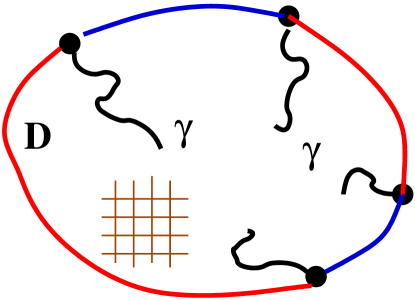
Figure 27: A domain $\mathbb{D}$ cutted along portions of interfaces.

Assuming the model to be at its critical point, we expect to be able to describe its continuum limit by a conformal field theory (CFT). At least for a wide class of observables $\mathcal{O}$, the partition function and statistical expectation values become CFT correlation functions:

$$\prec\mathcal{O}\succ_{\mathbb{D}}\to\frac{\langle\mathcal{O}\rangle_{\mathbb{D},\ b.c.}}{\langle{\bf I}\rangle_{\mathbb{D},\ b.c.}}$$

where $\langle\cdots\rangle_{\mathbb{D},\ b.c.}$ refer to the CFT correlation functions in the domain $\mathbb{D}$ with specific boundary conditions (b.c.). We need to write the correlation function of identity ${\bf I}$, proportional to the partition function $Z_{\mathbb{D}}$, in the denominator because the boundary conditions may already have led to insertions of boundary changing operators [26] that we have not mentioned explicitly. This partition function depends on the positions $x^{(j)}$ at which the boundary conditions have been changed.

With boundary condition changing at $N$ points $x^{(1)},\dots,x^{(N)}$ on the boundary, partitioning the configuration space amounts to specify portions of $N$ interfaces starting at these points. Denote by $\gamma_{[x^{(j)}\gamma_{T}^{(j)}]}$ these interfaces – starting at $x^{(j)}$ and ending at $\gamma^{(j)}_{T}$ – and by $\gamma_{T}$ their unions. As in previous Section, let $\mathcal{C}_{\gamma_{T}}$ be the set of configuration with interfaces $\gamma_{T}$. The statistical expectation $\prec\mathcal{O}\succ_{|\gamma_{T}}$ conditioned on $\gamma_{T}$ is identical to the statistical expectation on the domain $\mathbb{D}_{T}$ obtained from the original domain $\mathbb{D}$ by removing the interfaces $\gamma_{T}$. Thus, in the continuum and at criticality we expect that

$$\prec\mathcal{O}\succ_{|\gamma_{T}}\to\frac{\langle\mathcal{O}\rangle_{\mathbb{D}_{T},\ b.c}}{\langle{\bf I}\rangle_{\mathbb{D}_{T},\ b.c.}}\quad,\quad\mathbb{D}_{T}=\mathbb{D}\setminus\gamma_{T}$$

In the continuum limit, the interfaces may have double points so that they encircle a set of hulls $\mathbb{K}_{T}$. In that case $\mathbb{D}_{T}$ is $\mathbb{D}$ with the hulls (and not only the traces) removed.

For certain (but not all) observables, $\prec\mathcal{O}\succ_{\mathbb{D}}$ is computing a probability, which in a conformal field theory ought to be conformally invariant. But $\prec\mathcal{O}\succ_{\mathbb{D}}$ is written as a quotient, and this means that the numerator and denominator should transform homogeneously (and with the same factor) under conformal transformations. In particular, the denominator should transform homogeneously. This means that $\langle{\bf I}\rangle_{\mathbb{D},\ b.c.}$ – which depends on the position of the boundary condition changes – behaves like a product of boundary primary fields. Then, by locality, for any $\mathcal{O}$, the transformation of the numerator under conformal maps will split in two pieces: one containing the transformations of $\mathcal{O}$ and the other one canceling with the factor in the denominator. So we infer the existence in the CFT of a primary boundary field, denoted by $\psi(x)$ in what follows, which implements boundary condition changes at which interfaces anchor. Hence we may write

$$\langle{\bf I}\rangle_{\mathbb{D},\ b.c.}=\langle\psi(x^{(1)})\cdots\psi(x^{(N)})\rangle_{\mathbb{D}}$$

and

$$\langle\mathcal{O}\rangle_{\mathbb{D}}=\langle\mathcal{O}\psi(x^{(1)})\cdots\psi(x^{(N)})\rangle_{\mathbb{D}}.$$

Conformal invariance relates correlation in $\mathbb{D}_{T}$ and $\mathbb{D}$ provided they are conformally equivalent so that $\langle\mathcal{O}\rangle_{\mathbb{D}_{T}}$ possesses a simple expression in term $\langle\mathcal{O}\rangle_{\mathbb{D}}$. Write the transformation of the observable $\mathcal{O}$ as $g:\mathcal{O}\rightarrow\;^{g}\,\mathcal{O}$ under a conformal map $g$. Denote by $g_{T}$ a conformal representation of $g_{T}:\mathbb{D}_{T}\rightarrow\mathbb{D}$ and write $g_{T}(\gamma^{(j)}_{T})\equiv X^{(j)}_{T}$. The expression for the closed martingale $\prec\mathcal{O}\succ_{T}$ can then be simplified further

$$\prec\mathcal{O}\succ_{|\gamma_{T}}=\prec\mathcal{O}\succ_{\mathbb{D}_{T}}\to\frac{\langle\,^{g_{T}}\mathcal{O}\,\psi(X^{(1)}_{T})\cdots\psi(X^{(N)}_{T})\rangle_{\mathbb{D}}}{\langle\psi(X^{(N)}_{T})\cdots\psi(X^{(N)}_{T})\rangle_{\mathbb{D}}}.$$ (24)

with ${}^{g_{T}}\mathcal{O}$ the image of $\mathcal{O}$ by the map $g_{T}$. The CFT correlation functions are now defined on the original domain $\mathbb{D}$ but the insertion point $X_{T}^{(j)}$ have been moved by the uniformizing map $g_{T}$ which erase all the portions of the interfaces. The Jacobians coming from the transformations of the boundary changing primary field $\psi$ have canceled in the numerator and denominator. Of course, we have cheated a little. For the actual map $g_{T}$, which is singular at the $\gamma^{(j)}_{T}$’s, these Jacobians are infinite. A more proper derivation would go through a regularization but locality should ensure that the naive formula remains valid when the regularization is removed. Eq.(24) is the starting point of our analysis.

5.3 CFTs of SLEs: chordal case

In the continuum limit and at criticality the probability measure on interfaces (21) induced by the Boltzmann weight is expected to converge in an appropriate sense to a SLE measure. However, SLEs depend only an unique parameter $\kappa$ and details on the statistical model has been erased. The connection between SLE and the CFT representing the statistical model at criticality is restored by demanding that the condition expectations $\prec\mathcal{O}\succ_{|\gamma_{T}}$ represented in eq.(24) are SLE martingales. Imposing this relation constraints the CFT moduli as a function of the SLE parameters. The output of the derivation we shall explain next may be stated in simple words:

• SLEs with parameter $\kappa$ describe interfaces in CFTs of Virasoro central charge

  $$c_{\kappa}=\frac{(6-\kappa)(3\kappa-8)}{2\kappa}=1-6\frac{(\kappa-4)^{2}}{4\kappa}.$$ (25)

  Notice that $c_{\kappa}<1$ and that it is invariant under the duality $\kappa\leftrightarrow 16/\kappa$. Examples of correspondences are given below.

• The boundary conformal operator $\psi(x)$ implementing the change of boundary condition at the point on which the interface emerges has scaling dimension

  $$h_{1;2}=\frac{6-\kappa}{2\kappa}.$$ (26)

  It is a Virasoro primary operator degenerate at level two. In the CFT literature this field is often denoted $\psi_{1;2}$, a notation which makes references to the so-called Kac’s labels. See Appendix B for an explanation of this statement.

For chordal SLE there is only one interface so that there are only two boundary changing operators, one at the starting point $x_{0}$ and at the terminal point $x_{\infty}$ of the interface. If, as in previous Section, we cut the domain $\mathbb{D}$ along a portion of the interface and remove the corresponding hull $\mathbb{K}_{t}$, the boundary changing operators are then localized at the tip $\gamma_{t}$ of the hull and again at $x_{\infty}$. The correlation function in $\mathbb{D}_{t}$ are then:

$$\langle\mathcal{O}\rangle_{\mathbb{D}_{t},b.c.}=\langle\mathcal{O}\psi(x_{\infty})\psi(\gamma_{t})\rangle_{\mathbb{D}_{t}},\quad\psi\equiv\psi_{1;2}$$

Since the cutted domain $\mathbb{D}_{t}$ is conformally equivalent to $\mathbb{D}$, with the Loewner map $g_{t}$ intertwining the two domains, we may use conformal invariance to express these correlation functions as correlation functions in the original domain $\mathbb{D}$. Using the fact that $g_{t}(\gamma_{t})=U_{t}$, (with $U_{t}=\sqrt{\kappa}B_{t}$ if $\mathbb{D}=\mathbb{H}$), the statistical martingale (24) then becomes:

$$\prec\mathcal{O}\succ_{\mathbb{D}_{t}}=\frac{\langle^{g_{t}}\mathcal{O}\psi(x_{\infty})\psi(U_{t})\rangle_{\mathbb{D}}}{\langle\psi(x_{\infty})\psi(U_{t})\rangle_{\mathbb{D}}}$$ (27)

where ${}^{g_{t}}\mathcal{O}$ is the image of $\mathcal{O}$ under the conformal map $g_{t}$.

As explained below the fact that eq.(27) is a (local) martingale for chordal SLEs relies on second order differential equations satisfied by the CFT correlation functions with insertions of the boundary operators $\psi$. The correspondence between SLE and CFT thus relies on a identification of the Fokker-Planck like second order differential operators driving the SLE processes with the CFT differential equations – which are consequences of null vector relations satisfied by primary fields of specific representations of the Virasoro algebra.

5.3.1 SLE/CFT correspondence

We exemplify the SLE/CFT correspondence in a few specific cases. Let us start with the example considered in original Schramm’s paper: loop erased random walk (LERW). There [118, 95], it was shown that LERW does correspond to SLE with $\kappa=2$ and so to CFT with central charge $c=-2$ – a very special and simple CFT. The proof relies first in establishing that LERW satisfies the domain Markov property, at least in the continuum limit, and second in proving by estimating some observables that the driving Loewner process converges to a Brownian motion. The dual value $\kappa=8$, which is the marginal case in the space-filling phase, describes uniform spanning trees [81].

As shown by Smirnov’s [125], critical percolation corresponds to $\kappa=6$ and vanishing central charge. The dual value $\kappa=8/3$ is expected to describe self avoiding random walk (SAW), although there is no complete mathematical proof yet, but see ref.[96].

Boundaries of Ising spin clusters are conjectured to be described by SLE at $\kappa=3$ and central charge $1/2$. The boundary operator $\psi_{1;2}$, which then codes for the change of boundary conditions from $+$ spins to $-$ spins, has dimension $1/2$.

The $Q$-state Potts models correspond to $Q=4\cos^{2}(4\pi/\kappa)$ with $4\leq\kappa<8$, see ref.[7]. The SLE traces are expected to describe the continuum limit of the boundary of the Fortuin-Kastelyn [61] clusters arising in the hight temperature expansion of the Potts models. The $Q=2$ Potts model represents the Ising model, it corresponds to the dual value $\kappa=16/3$.

The self dual value $\kappa=4$ is special in the sense that it corresponds to a Gaussian massless free field with central charge $1$. Assuming Dirichlet boundary conditions, the SLE curves may be thought as discontinuity curves of the free field. The curves start from the boundary point at which the Dirichlet boundary conditions jump by a specific amount so that this discontinuity propagates inside the domain. The mathematical proof that such discontinuity line exists almost surely for each realization of the Gaussian field is not so simple as a Gaussian free field is actually a distribution and not a function. This was nevertheless done is ref.[122] by taking the scaling limit of discrete model. A relation with domino tiling is described in refs.[79, 80].

There are two phases in the critical $O(n)$ models [108, 109, 25]: the dilute and the dense phase. Parameterizing $n$ as $n=-2\cos(\pi g)$, the two values $g$ and $2-g$ give the same value of $n$ but $1\leq g\leq 2$ corresponds to the dilute phase while $0\leq g\leq 1$ to the dense phase. The relation with $O(n)$ loops and SLE is via $g=4/\kappa$ so that the dense phase is for $4\leq\kappa\leq 8$ and the dilute phase for $2\leq\kappa\leq 4$. This is in accordance with the SLE phases. The $O(n=1)$ model corresponds in the dilute phase to the Ising model with $g=4/3$ ($\kappa=3,\ c=1/2$) and in the dense phase to percolation with $g=2/3$ ($\kappa=6,\ c=0$). The $O(n=0)$ model describes in the dilute phase self avoiding walk (SAW) with $g=3/2$ ($\kappa=8/3,\ c=0)$ and in the dense phase uniform spanning trees (UST) with $g=1/2$ ($\kappa=8,\ c=-2$). Loop erased random walk (LERW) corresponds to the $O(n=-2)$ in the dilute phase with $g=2$ ($\kappa=2,\ c=-2$). There is no $O(n)$ models corresponding to $\kappa\in[0,2[$.

In conformal field theory these correspondences were predicted some time ago using the coulomb gas representation of the $O(n)$ models [108, 109, 83, 25]. The basic ingredients of these correspondences are as follows. Recall from Section 2 that the lattice $O(n)$ models may be presented as a loop gas model. The first step towards the coulomb gas representation consists in introducing a field $\phi$ at each site of the dual lattice. There is then a one-to-one mapping between configurations of the oriented loops and of the field. The rules are as follows: fix $\phi=0$ on the boundary and increase (decrease) $\phi$ by a fixed amount, say $\pi$, each time a loop is crossed which goes to the left (right). The fact that the loops are closed makes this procedure consistent. In the scaling limit, $\phi$ takes continuous values and the $O(n)$ lines are identified with the level lines of $\phi$. They form a set of non-intersecting loops. These level lines are also the current lines of the current $j^{\mu}=\epsilon^{\mu\nu}\partial_{\nu}\phi$ so that the direction of the current orientates the loops. The boundary condition ensures that the loop cannot cross the boundary. The last but crucial step consists in arguing that the action of $\phi$, which gives the weight of each loop configuration, renormalizes to that of a Gaussian free field with a background charge at infinity [108, 109, 25].

5.3.2 Correlation functions

This Section aims at giving a proof of the SLE/CFT correspondence using properties of CFT correlation functions. The main point consists in proving that for an appropriate choice of the CFTs and the boundary condition changing operators $\psi$ the ratios of correlation functions (27) are local martingales. This amounts to check that there is no drift term in their Itô derivative.

For simplicity we deal with chordal SLE in the upper half plane $\mathbb{H}$ with $x_{0}=0$ and $x_{\infty}=\infty$. The boundary operator localized at infinity creates a state, which we denote by $\langle\psi_{1;2}|$, and the two point function $\langle\psi(x_{\infty})\psi(\xi_{t})\rangle_{\mathbb{H}}$ becomes trivial so that the statistical martingale (27) reduces to the CFT correlation function:

$$\langle\mathcal{O}\rangle_{\mathbb{H}_{t}}=\langle\psi_{1;2}|^{g_{t}}\mathcal{O}\,\psi(\xi_{t})|0\rangle$$ (28)

with $|0\rangle$ the conformal vacuum. To simplify further we only sketch the computation when the operator $\mathcal{O}$ is a product of an arbitrary number $l$ of boundary primary fields $\mathcal{O}=\prod_{\alpha=1}^{l}\varphi_{\delta_{\alpha}}(Y^{(\alpha)})$ at positions $Y^{(\alpha)}$ and with scaling dimensions $\delta_{\alpha}$. The insertion points $Y^{(\alpha)}$ are away from the boundary changing operators $\psi$. This operator transform covariantly under conformal map so that:

$${}^{g_{t}}\mathcal{O}=\prod_{\alpha=1}^{l}\Big{[}\,g^{\prime}_{t}(Y^{(\alpha)})^{\delta_{\alpha}}\cdot\varphi_{\delta_{\alpha}}(g_{t}(Y^{(\alpha)}))\,\Big{]}$$ (29)

The Loewner map $g_{t}$ is regular with positive derivative at the insertion points $Y^{(\alpha)}$. Substitution of ${}^{g_{t}}\mathcal{O}$ in formula (28) yields:

$$\langle\mathcal{O}\rangle_{\mathbb{H}_{t}}=\prod_{\alpha=1}^{l}g^{\prime}_{t}(Y^{(\alpha)})^{\delta_{\alpha}}\cdot\langle\psi_{1;2}|\prod_{\alpha=1}^{l}\varphi_{\delta_{\alpha}}(g_{t}(Y^{(\alpha)}))\,\psi(\xi_{t})|0\rangle$$

We shall denote by $J_{t}^{\varphi}=\prod_{\alpha=1}^{l}g^{\prime}_{t}(Y^{(\alpha)})^{\delta_{\alpha}}$ is the Jacobian and by $Z_{\mathbb{H}_{t}}^{\varphi}$ the CFT correlation function.

We need to compute the Itô derivative of $\langle\mathcal{O}\rangle_{\mathbb{H}_{t}}$. Ito’s formula for the $\psi$’s gives

$$d\psi(\xi_{t})=\psi^{\prime}(\xi_{t})d\xi_{t}+\frac{\kappa}{2}\psi^{\prime\prime}(\xi_{t})dt.$$

Using the Loewner equation for $g_{t}(z)$ and its derivative with respect to $z$, one checks that

$$d\left(\varphi_{\delta}(g_{t}(Y))g^{\prime}_{t}(Y)^{\delta}\right)=2g^{\prime}_{t}(Y)^{\delta}\left(\frac{\varphi^{\prime}_{\delta}(g_{t}(Y))}{g_{t}(Y)-\xi_{t}}-\delta\frac{\varphi_{\delta}(g_{t}(Y))}{(g_{t}(Y)-\xi_{t})^{2}}\right)dt.$$ (30)

The time $t$ being given, we can simplify the notation. Set $x\equiv\xi_{t}$ and $y_{\alpha}\equiv g_{t}(Y^{(\alpha)})$ and view $Z^{\varphi}_{\mathbb{H}_{t}}$ as a function of $y_{\alpha}$ and $x$. From the chain rule we get

$$d(Z_{\mathbb{H}_{t}}^{\varphi}J^{\varphi}_{t}) = {J^{\varphi}_{t}}\,\left[d\xi_{t}\partial_{x}+dt\left(\frac{\kappa}{2}\partial_{x}^{2}+2\sum_{\alpha}\left[\frac{1}{y_{\alpha}-x}\partial_{y_{\alpha}}-\frac{\delta_{\alpha}}{(y_{\alpha}-x)^{2}}\right]\right)\right]Z_{\mathbb{H}_{t}}^{\varphi}$$

The left hand side defines the differential operators driving the SLE processes. Thus, the drift term in the Itô derivative of the putative martingale vanishes if and only if

$$\left(\frac{\kappa}{2}\partial_{x}^{2}+2\sum_{\alpha}\left[\frac{1}{y_{\alpha}-x}\partial_{y_{\alpha}}-\frac{\delta_{\alpha}}{(y_{\alpha}-x)^{2}}\right]\right)Z_{\mathbb{H}_{t}}^{\varphi}=0.$$ (31)

This is a standard example of differential equation fulfills by CFT correlation functions. It should hold true for any number of insertions of primary operators $\varphi_{\delta_{\alpha}}$. This implies that $\psi$ is a degenerate field with a vanishing descendant at level two and conformal weight $h_{1;2}=\frac{6-\kappa}{2\kappa}$. The central charge is $c_{\kappa}=\frac{(6-\kappa)(3\kappa-8)}{2\kappa}$. See Appendix B for further information on degenerate field in conformal field theories.

5.3.3 Operator formalism

The aim of this Section is to derive the SLE/CFT correspondence using the CFT operator formalism which was initially developed in ref.[6, 7, 9]. This will reveal deep relation between SLEs and special representations of the Virasoro algebra.

We start with the group theoretical formulation of chordal SLE as explained in Section 4.4. Recall that $h_{t}(z)\equiv g_{t}(z)-\xi_{t}$ satisfies the stochastic differential equation $dh_{t}={2dt}/{h_{t}}-d\xi_{t}.$ According to Section 4.4.2, to $h_{t}$ we can associate $\mathfrak{g}_{h_{t}}\in N_{-}$, with $N_{-}$ the group of germs of holomorphic functions at $\infty$ of the form $z+\sum_{m\leq-1}h_{m}z^{m+1}$. By Itô’s formula, it satisfies:

$$\mathfrak{g}_{h_{t}}^{-1}\cdot d\mathfrak{g}_{h_{t}}=dt(-2\ell_{-2}+\frac{\kappa}{2}\ell_{-1}^{2})+d\xi_{t}\ell_{-1}.$$ (32)

with $\ell_{-2}=-z^{-1}\partial_{z}$ and $\ell_{-1}=-\partial_{z}$. Compare with eq.(17).

In conformal field theory the operators $\ell_{n}=-z^{n+1}\partial_{z}$, with $[\ell_{m},\ell_{n}]=(m-n)\ell_{m+n}$, are represented by operators $L_{n}$ which satisfy the Virasoro algebra $\mathfrak{vir}$:

$$[L_{m},L_{n}]=(m-n)L_{m+n}+\frac{c}{12}m(m^{2}-1)\delta_{m+n;0}$$

with $c$ the Virasoro central charge. See Appendix B for the necessary information on the Virasoro algebra and its representations. We need to introduce the notation $\mathfrak{n}_{-}$ for the sub-algebra of $\mathfrak{vir}$ generated by the $L_{n}$’s with $n<0$. In the following we shall only deal with highest weight representations. These are representations of $\mathfrak{vir}$ which possess a highest weight vector $|h\rangle$ are such that $L_{n}|h\rangle=0$ for $n>0$ and $L_{0}|h\rangle=h|h\rangle$. The parameter $h$ is called the conformal dimension of the representation.

The representations of $\mathfrak{vir}$ are not automatically representations of $N_{-}$, one of the reasons being that the Lie algebra of $N_{-}$ contains infinite linear combinations of the generators $\ell_{n}$’s. However, as explained in ref.[9, 11], highest weight representations of $\mathfrak{vir}$ can be extended in such a way that $N_{-}$ get embedded in a appropriate completion $\overline{\mathcal{U}(\mathfrak{n}_{-})}$ of the enveloping algebra of the sub-algebra $\mathfrak{n}_{-}$ of $\mathfrak{vir}$. This allows to associate to any $\mathfrak{g}_{h}\in N_{-}$ an operator $G_{h}$ acting on appropriate representations of $\mathfrak{vir}$ and satisfying $G_{g\circ f}=G_{f}\cdot G_{g}$ so that the map $\mathfrak{g}_{h}\to G_{h}$ is a homomorphism.

One may think about $G_{h}$ as the operator implementing the conformal map $h(z)$ of the form $z+\sum_{m\leq-1}h_{m}z^{m+1}$ in the Virasoro representations and thus in the CFT Hilbert spaces. In particular if $\varphi_{\delta}(Y)$ is a boundary primary field of scaling dimension $\delta$ acting on the representations of $\mathfrak{vir}$ then $G_{h}$ acts by conjugaison as:

$$G^{-1}_{h}\,\varphi_{\delta}(Y)\,G_{h}=|h^{\prime}(Y)|^{\delta}\,\varphi_{\delta}(h(Y))$$

More generally, the image ${}^{h}\mathcal{O}$ of an operator $\mathcal{O}$ by the conformal map $h$ is obtained by conjugating it by the operator $G_{h}$ as standard rules of quantum mechanics tells us: ${}^{h}\mathcal{O}=G^{-1}_{h}\,\mathcal{O}\,G_{h}$. In particular, $G_{h}$ acts on the CFT stress tensor $T(z)=\sum_{n}L_{n}z^{n-2}$ as:

$$G_{h}^{-1}\,T(z)\,G_{h}=T(h(z))\,h^{\prime}(z)^{2}+\frac{c}{12}\,Sh(z),$$ (33)

with $Sh(z)=(\frac{h^{\prime\prime}}{h^{\prime}})^{\prime}-\frac{1}{2}(\frac{h^{\prime\prime}}{h^{\prime}})^{2}$ the Schwarzian derivative of $h$. This extra term reflects the anomalous transformation law of the CFT stress tensor under conformal transformations [21].

Implementing this construction for the random Loewner map $h_{t}$ yields random operators $G_{h_{t}}\in\overline{\mathcal{U}(\mathfrak{n}_{-})}$ which satisfy the stochastic Itô equation [6, 7]:

$$G_{h_{t}}^{-1}dG_{h_{t}}=dt(-2L_{-2}+\frac{\kappa}{2}L_{-1}^{2})+d\xi_{t}L_{-1}.$$ (34)

This follows directly from eq.(17) and the fact that the correspondence $\mathfrak{g}_{h}\to G_{h}$ is a homomorphism. This may be viewed as defining a Markov process in the enveloping algebra $\overline{\mathcal{U}(\mathfrak{n}_{-})}$.

Eq.(34) does not contain more information than eq.(17), or than the Loewner equation, but it now makes sense in the CFT Hilbert spaces. This immediatly leads to the following important result:

• Let $|\psi_{1;2}\rangle$ be the highest weight vector in the irreducible highest weight representation (degenerate at level two) of $\mathfrak{vir}$ of central charge $c_{\kappa}=\frac{(6-\kappa)(3\kappa-8)}{2\kappa}$ and conformal weight $h_{1;2}\equiv\frac{6-\kappa}{2\kappa}$.
  Then $G_{h_{t}}|\psi_{1;2}\rangle$ is a local martingale.

• Assuming appropriate boundedness conditions on $\langle v|$, the scalar product $\langle v|G_{h_{t}}|\psi_{1;2}\rangle$ is a martingale so that ${\mathbf{E}}\left[\langle v|G_{h_{t}}|\psi_{1;2}\rangle|\{{G_{h_{u}}}\}_{u\leq s}\right]$ is time independent for $t\geq s$ and:

  $${\mathbf{E}}\left[\,\langle v|G_{h_{t}}|\psi_{1;2}\rangle\,\big{|}\{G_{h_{u}}\}_{u\leq s}\right]=\langle v|G_{h_{s}}|\psi_{1;2}\rangle$$ (35)

  In particular, $\langle v|G_{h_{t}}|\psi_{1;2}\rangle$ is conserved in mean for any $\langle v|$.

This result is a direct consequence of eq.(34) and the null vector relation at level two, $(-2L_{-2}+\frac{\kappa}{2}L_{-1}^{2})|\psi_{1;2}\rangle=0$, so that $dG_{h_{t}}|\psi_{1;2}\rangle=G_{h_{t}}L_{-1}|\psi_{1;2}\rangle d\xi_{t}$. The null vector condition is what fixes the values of the conformal weight and of the central charge.

Since $G_{h_{t}}$ is the operator intertwining the conformal field theories in $\mathbb{H}$ and in the random domain $\mathbb{H}_{t}$, this result has the following important consequences. Consider CFT correlation functions in $\mathbb{H}_{t}$. They can be computed by looking at the same theory in $\mathbb{H}$ modulo the insertion of an operator representing the deformation from $\mathbb{H}$ to $\mathbb{H}_{t}$. This operator is $G_{h_{t}}$. Recall the expression (28) of expectation values in the upper half plane with the hull removed which, after translating by $\xi_{t}$ to go from $g_{t}$ to $h_{t}=g_{t}-\xi_{t}$, can be written as:

$$\langle\mathcal{O}\rangle_{\mathbb{H}_{t}}=\langle\psi_{1;2}|\,^{h_{t}}\mathcal{O}\,\psi(0)|0\rangle.$$

The boundary operator $\psi\equiv\psi_{1;2}$ with dimension $\frac{6-\kappa}{2\kappa}$ is the operator which create the highest weight vector $|\psi_{1;2}\rangle$ at the tip of the hull, so that $\psi(0)|0\rangle=|\psi_{1;2}\rangle$. Using ${}^{h_{t}}\mathcal{O}=G^{-1}_{h_{t}}\mathcal{O}G_{h_{t}}$ we get:

$$\langle\mathcal{O}\rangle_{\mathbb{H}_{t}}=\langle\psi_{1;2}|\mathcal{O}\,G_{h_{t}}|\psi_{1;2}\rangle$$ (36)

where we use $\langle\psi_{1;2}|G^{-1}_{h_{t}}=\langle\psi_{1;2}|$ since $G_{h_{t}}$ is the operator implementing a conformal map fixing infinity and with derivative $1$ at infinity.

Suppose now that the central charge is $c=(6-{\kappa})(3\kappa-8)/2\kappa$, then $\langle\mathcal{O}\rangle_{\mathbb{H}_{t}}$ is a local martingale because so is $G_{h_{t}}|\psi_{1;2}\rangle$. In particular, the correlation functions of the conformal field theory in the fluctuating geometry $\mathbb{H}_{t}$ are in average time independent:

$${\mathbf{E}}\left[\langle\mathcal{O}\rangle_{\mathbb{H}_{t}}\right]=\langle\mathcal{O}\rangle_{\mathbb{H}},$$

a result that we also found by computing directly the CFT correlation functions in the previous Section.

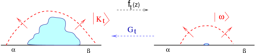
Figure 28: A representation of the boundary hull state $|K_{t}\rangle=G_{h_{t}}|\psi_{1;2}\rangle$ and of the map intertwining different formulations of the CFT.

The state $G_{h_{t}}|\psi_{1;2}\rangle$ may be interpreted as follows. Imagine defining the conformal field theory in $\mathbb{H}_{t}$ via a radial quantization, so that the conformal Hilbert spaces are defined over curves topologically equivalent to half circles around the origin. Then, the SLE hulls manifest themselves as disturbances localized around the origin, and as such they generate states in the conformal Hilbert spaces. Since $G_{h_{t}}$ intertwines the CFT in $\mathbb{H}$ and in $\mathbb{H}_{t}$, these states are $G_{h_{t}}|\psi_{1;2}\rangle$ with $|\psi_{1;2}\rangle$ keeping track of the boundary conditions. See Fig.28.

The operator formalism shows directly that the state $G_{h_{t}}|\psi_{1;2}\rangle$ is a generating function of local martingales, since it may be expanded on any appropriate basis. This was used in ref.[8] to show that the vector space of martingale polynomials in the Taylor coefficients of the Loewner map $h_{t}$ carries a representation of the Virasoro algebra. Explicit expressions of the Virasoro generators acting on this space were given in terms of differential operators so that all polynomial martingales can be obtained by iterative applications of these differential operators.

5.4 Other SLEs

The aim of this Section is to extend the SLE/CFT correspondence to the other SLEs. Again the correspondence is attached to the construction of SLE martingales using tools from CFT. As in the chordal case we can use either a formalism based on correlation function or an operator formalism.

In the correlation function formalism, we shall identify the statistical martingales as ratio of CFT correlation functions:

$$\prec\mathcal{O}\succ_{\mathbb{D}_{t}}=\frac{\langle\mathcal{O}\rangle_{\mathbb{D}_{t},b.c.}}{\langle{\bf I}\rangle_{\mathbb{D}_{t},b.c.}}$$

What distinguished the different SLEs are the different boundary conditions which depends on the marked points specific to each SLEs and on the behavior of the SLEs map in the neighborhood of these points. This translates into the insertions of appropriate boundary and/or bulk operators in the CFT correlation functions.

In the operator formalism we start from the stochastic equation (16) satisfied by the group element $\mathfrak{g}_{h_{t}}$ associated to the Loewner map. As for the chordal case, this element is then promoted to an operator $G_{h_{t}}$ acting on representations of the Virasoro algebra and thus acting on CFT Hilbert spaces. The operator $G_{h_{t}}$ is the operator which intertwines the conformal field theories in the domain $\mathbb{D}$ and in the domain $\mathbb{D}_{t}$ with the hull removed so that ${}^{h_{t}}\mathcal{O}=G_{h_{t}}^{-1}\mathcal{O}G_{h_{t}}$ for any operator $\mathcal{O}$. By construction it satisfies an equation analogous to eq.(16) of the following form:

$$G_{h_{t}}^{-1}\cdot dG_{h_{t}}=dt\,(-2W_{-2}+\frac{\kappa}{2}W_{-1}^{2})+d\xi_{t}\,W_{-1},$$ (37)

with $W_{-2}$ and $W_{-1}$ elements of the Virasoro algebra. Their precise forms depend on the type of SLE we are considering.

5.4.1 Radial SLE

Radial SLE describes curves in a domain $\mathbb{D}$ starting from a boundary point $x_{0}$ and ending at a bulk point $z_{*}$. The CFT correlation functions take into account these boundary conditions by the insertion a boundary field $\psi$, which is going to be $\psi_{1;2}$ as in the chordal case, at the tip of the curve and a bulk field, which we shall soon identify as $\Phi_{0;1/2}$, at the bulk point. Thus:

$$\langle\mathcal{O}\rangle_{\mathbb{D}_{t},b.c.}=\langle\mathcal{O}\,\Phi_{0;1/2}(z_{*})\psi(\gamma_{t})\rangle_{\mathbb{D}_{t}}$$

Similarly the conditioned partition function is $\langle{\bf I}\rangle_{\mathbb{D}_{t},b.c.}=\langle\Phi_{0;1/2}(z_{*})\psi(\gamma_{t})\rangle_{\mathbb{D}_{t}}$. By definition of the radial SLE map $g_{t}$, the tip of the curve is mapped to the driving process $U_{t}=g_{t}(\gamma_{t})$ and the terminal bulk point $z_{*}$ is fixed by $g_{t}$. Thus for radial SLE the statistical martingale reads:

$$\prec\mathcal{O}\succ_{\mathbb{D}_{t}}=\frac{\langle^{g_{t}}\mathcal{O}\,\Phi_{0;1/2}(z_{*})\psi(U_{t})\rangle_{\mathbb{D}}}{\langle\Phi_{0;1/2}(z_{*})\psi(U_{t})\rangle_{\mathbb{D}}}$$ (38)

It is then a matter a simple computation – which we leave to the reader but which is very much parallel to the one done for the chordal case in the previous Section – to verify that the above expectation values is a SLE martingale provided that [10]:

• the boundary operator $\psi$ is the boundary primary operator $\psi_{1;2}$ degenerate at level two with scaling dimension $h_{1;2}=\frac{6-\kappa}{2\kappa}$;

• the bulk operator $\Phi_{0;1/2}$ is a spinless primary operator with scaling dimension $2h_{0;1/2}=\frac{(\kappa-2)(6-\kappa)}{8\kappa}$.

As in the chordal case, the martingale property for $\prec\mathcal{O}\succ_{\mathbb{D}_{t}}$ essentially relies on the differential equation satisfied by CFT correlation functions with insertion of the degenerate operator $\psi$. The need for the insertion of the bulk operator $\Phi_{0;1/2}$ at the point where the SLE curves terminate is in agreement with the identification of the operators $\Phi_{0;n/2}$ as those testing for the presence of $n$ SLE traces in the neighborhood of a bulk point. See Section 7.

The SLE/CFT correspondence may also be done using the operator formalism. Let $G_{h_{t}}$ be the operator representing the action of $\mathfrak{g}_{h_{t}}$ in the CFT Hilbert spaces for radial SLE. It satisfies eq.(37). We look at radial SLE in the upper half plane geometry. The Loewner equation is then given in eq.(18). We have seen in Section 4.4 that $w_{-1}=\frac{1}{2}(\ell_{-1}+\ell_{1})$ and $w_{-2}=\frac{1}{4}(\ell_{-2}+\ell_{0})$, so that

$$W_{-1}=\frac{1}{2}(L_{-1}+L_{1}),\qquad W_{-2}=\frac{1}{4}(L_{-2}+L_{0}).$$

A simple rearrangement leads to $(-2W_{-2}+\frac{\kappa}{2}W_{-1}^{2})|\psi_{1;2}\rangle=2h_{0;1/2}|\psi_{1;2}\rangle$. From eq.(37) we then deduce that $G_{h_{t}}^{-1}dG_{h_{t}}|\psi_{1;2}\rangle=2h_{0;1/2}|\psi_{1;2}\rangle+d\xi_{t}W_{-1}|\psi_{1;2}\rangle$ and thus that

$$e^{-2h_{0;1/2}t}G_{h_{t}}|\psi_{1;2}\rangle$$

is a local martingale. The prefactor $e^{-2h_{0;1/2}t}$ accounts for the insertion of a bulk conformal field of scaling dimension $2h_{0;1/2}$ localized at the fixed point. See ref.[10] for further details.

The radial SLE is for instance well adapted to the $O(n)$ models with the insertion of the operators $\psi_{1;2}$ and $\Phi_{0;1/2}$ conditioning on the presence of an $O(n)$ trace from their boundary and bulk insertion points.

5.4.2 Dipolar SLE

Dipolar SLE describes curves in a domain $\mathbb{D}$ starting from a boundary point $x_{0}$ and stopped the first instant it hits a boundary interval $[x_{-},x_{+}]$ excluding the starting point. The CFT correlation functions take into account these boundary conditions by the insertion a boundary field $\psi$, which creates the SLE trace, at the tip of the curve and two other boundary fields, which we shall soon identify as $\psi_{0;1/2}$, at the two marked points $x_{\pm}$. Thus we expect:

$$\langle\mathcal{O}\rangle_{\mathbb{D}_{t},b.c.}=\langle\mathcal{O}\,\psi_{0;1/2}(x_{-})\psi_{0;1/2}(x_{+})\psi(\gamma_{t})\rangle_{\mathbb{D}_{t}}$$

By definition of the radial SLE map $g_{t}$, the tip of the curve is mapped to the driving process $U_{t}=g_{t}(\gamma_{t})$ and the marked boundary points $x_{\pm}$ fixed by $g_{t}$. Thus for dipolar SLE the statistical martingales read:

$$\prec\mathcal{O}\succ_{\mathbb{D}_{t}}=\frac{\langle^{g_{t}}\mathcal{O}\,\psi_{0;1/2}(x_{-})\psi_{0;1/2}(x_{+})\psi(U_{t})\rangle_{\mathbb{D}}}{\langle\psi_{0;1/2}(x_{-})\psi_{0;1/2}(x_{+})\psi(U_{t})\rangle_{\mathbb{D}}}$$ (39)

Again as for radial SLE, it is then a matter of a simple computation – which we leave to the reader – to verify that the above expectation values are SLE martingales provided that [13]:

• the boundary operator $\psi$ creating the SLE trace is the boundary primary operator $\psi_{1;2}$ degenerate at level two with scaling dimension $h_{1;2}=\frac{6-\kappa}{2\kappa}$;

• the two boundary operators $\psi_{0;1/2}$ at the two marked points have each scaling dimension $h_{0;1/2}=\frac{(\kappa-2)(6-\kappa)}{16\kappa}$.

As it is now usual, the martingale property for $\prec\mathcal{O}\succ_{\mathbb{D}_{t}}$ essentially relies on the differential equation satisfied by CFT correlation functions with insertion of the degenerate operator $\psi$.

We now describe the operator formalism for dipolar SLE. Let $G_{h_{t}}$ be the operator representing the action of $\mathfrak{g}_{h_{t}}$ in the CFT Hilbert spaces for dipolar SLE. It satisfies eq.(37). We look at dipolar SLE in the upper half plane geometry. The Loewner equation is then given in eq.(19). We have seen in Section 4.4 that $w_{-1}=\frac{1}{2}(\ell_{-1}-\ell_{1})$ and $w_{-2}=\frac{1}{4}(\ell_{-2}-\ell_{0})$, so that

$$W_{-1}=\frac{1}{2}(L_{-1}-L_{1}),\qquad W_{-2}=\frac{1}{4}(L_{-2}-L_{0}).$$

A simple computation leads to $(-2W_{-2}+\frac{\kappa}{2}W_{-1}^{2})|\psi_{1;2}\rangle=-2h_{0;1/2}|\psi_{1;2}\rangle.$ As for radial SLE, this together with eq.(37) immediately imply that

$$e^{+2h_{0;1/2}t}G_{h_{t}}|\psi_{1;2}\rangle$$

is a local martingale. The prefactor $e^{+2h_{0;1/2}t}$ accounts for the insertion of two boundary conformal fields, each of dimension $h_{0;1/2}$, localized at the two fixed points.

In the Ising model $(\kappa=3)$, for instance, $\psi_{1;2}$ of dimension $1/2$ corresponds to change from $+$ to $-$ boundary conditions while $\psi_{0;1/2}$ of dimension $1/16$ corresponds to change from free to $+$ (or to $-$) boundary conditions. So dipolar SLE at $\kappa=3$ describes Ising model with boundary conditions changing from $+$ to $-$ to free and back to $+$ along the boundary.

5.4.3 SLE($\kappa,\rho)$

As explained in Section 4.3.3, SLE($\kappa,\rho$) may be viewed as dipolar SLE but with an extra drift in the driving source. So the SLE/CFT correspondence is analogous [84] to that for dipolar SLE except that one has to change the nature of the boundary operator inserted at the two marked point $x_{\pm}$ kepted fix by the Loewner map. Thus we expect that:

$$\langle\mathcal{O}\rangle_{\mathbb{D}_{t},b.c.}=\langle\mathcal{O}\,\psi_{h_{-}}(x_{-})\psi_{h_{+}}(x_{+})\psi(\gamma_{t})\rangle_{\mathbb{D}_{t}}$$

The SLE($\kappa,\rho)$ statistical martingales similarly read:

$$\prec\mathcal{O}\succ_{\mathbb{D}_{t}}=\frac{\langle^{g_{t}}\mathcal{O}\,\psi_{h_{-}}(x_{-})\psi_{h_{+}}(x_{+})\psi(U_{t})\rangle_{\mathbb{D}}}{\langle\psi_{h_{-}}(x_{-})\psi_{h_{+}}(x_{+})\psi(U_{t})\rangle_{\mathbb{D}}}$$ (40)

As proved in [84], the above expectation values are SLE martingales provided that:

• the boundary operator $\psi$ creating the SLE trace is again the primary operator $\psi_{1;2}$ degenerate at level two with scaling dimension $h_{1;2}=\frac{6-\kappa}{2\kappa}$;

• the boundary operators $\psi_{h_{-}}$ and $\psi_{h_{+}}$ have scaling dimensions $h_{+}=\frac{\rho(\rho+4-\kappa)}{4\kappa}$ and $h_{-}=\frac{(\rho+2)(\rho+6-\kappa)}{4\kappa}$.

The conformal dimensions $h_{\pm}$ have a clear CFT interpretation. They are the generic dimensions of the primary operators satisfying the fusion rules with $\psi_{1;2}$ such that the three point function $\langle\psi_{h_{-}}(x_{-})\psi_{h_{+}}(x_{+})\psi_{1;2}(x_{0})\rangle_{\mathbb{D}}$ is non vanishing. They satisfy

$$h_{+}-h_{-}=\alpha/\kappa\quad,\quad h_{+}+h_{-}=2h_{0;1/2}+\alpha^{2}/2\kappa$$

with $\alpha=\frac{6-\kappa}{2}+\rho$ the drift coefficient in the driving source $U_{t}=\sqrt{\kappa}B_{t}+\alpha\,t$, see eq.(12).

The operator formalism for SLE$(\kappa,\rho)$ also follows directly from that of dipolar SLE since the vector fields $w_{-2}$ and $w_{-1}$ of SLE$(\kappa,\rho)$ are obtained from those of dipolar SLE by a translation, see Section 4.3.3:

$$W_{-2}^{{\rm SLE}(\kappa,\rho)}=W_{-2}^{\rm dip.}-\frac{\alpha}{2}\,W_{-1}^{\rm dip.}\quad,\quad W_{-1}^{{\rm SLE}(\kappa,\rho)}=W_{-1}^{\rm dip.}$$

As a consequence, the state

$$Z^{-1}_{t}\,G_{h_{t}}|\psi_{1;2}\rangle,\quad{\rm with}\quad Z^{-1}_{t}=\exp{[(2h_{0;1/2}+\frac{\alpha^{2}}{2\kappa})t-\frac{\alpha}{\sqrt{\kappa}}B_{t}]}$$

is a local martingale. The extra term $Z^{-1}_{t}$ takes into account the insertion of two operators $\psi_{h_{\pm}}$ in the partition function $\langle\psi_{h_{-}}(x_{-})\psi_{h_{+}}(x_{+})\psi_{1;2}(U_{t})\rangle_{\mathbb{H}}$. The microscopic interpretation of $SLE(\kappa,\rho)$ in terms of lattice statistical models is less clear but a few hints have been given in ref.[33].

5.5 Multiple SLEs

Multiple SLEs describe the local growth of $n$ interfaces in critical models, ie. in CFT, joining fixed points on the boundary by a Loewner chain with random driving source. See Fig.29. The first attempt – however not complete – to define them was done in [32]. A very interesting appraoch based on commutativity of the growths of the interfaces has then been developed in ref.[48, 49]. We shall instead follow the approach of ref.[14] which is based on implementing the statistical martingale trick to constrain the processes driving the growth of the traces. We assume that $0\leq\kappa<8$.

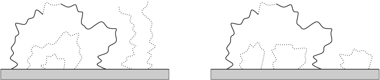
Figure 29: A representation of two configurations of growing curves forming arches whenever they touch themself.

5.5.1 The basic equations

We list here the set of necessary conditions and equations defining multiple SLEs. By conformal invariance, it is enough to give its definition when the domain is the upper half plane $\mathbb{H}$. The curves, labeled by an integer $i=1,\cdots,n$ and starting at position $X_{i}$, generate a hull whose complement is uniformized by a map $g_{t}$, which we assume to be hydrodynamically normalized at infinity as for a single chordal SLE. Since the hull is generated by $n$ curves, this map satisfies a Loewner equation with $n$ simple poles:

$$dg_{t}(z)=\sum_{i=1}^{n}\frac{2a^{(i)}_{t}dt}{g_{t}(z)-X^{(i)}_{t}}.$$ (41)

The initial condition is $g_{0}(z)=z$. The positive function $a^{(i)}_{t}$ parameterizes the speed of growth of the $i^{\rm th}$ curve. We normalize them by $\sum_{i}a^{(i)}_{t}=1$ so that the total capacity of the growing hulls at time $t$ is $2t$.

The processes $X^{(i)}_{t}$, which are the images of the tips of the curves by $g_{t}$, are solutions of the stochastic differential equations:

$$dX^{(i)}_{t}=d\xi^{(i)}_{t}+\kappa a^{(i)}_{t}dt\,(\partial_{x_{i}}\log Z)(X_{\cdot})+\sum_{j\neq i}\frac{2a^{(j)}_{t}dt}{X^{(i)}_{t}-X^{(j)}_{t}}.$$ (42)

with $d\xi^{(i)}_{t}=\sqrt{\kappa a_{t}^{(i)}}\,dB_{t}^{(i)}$ where $B_{t}^{(i)}$ are $n$ independent normalized Brownian motions. This choice ensures that the curves grow locally as SLE traces. The initial conditions are $X_{0}^{(i)}=X_{i}$ ordered in such a way that $X_{1}<X_{2}<\cdots<X_{n}$.

The system depends on a function $Z(x_{1},\cdots,x_{n})$ which reflect the interactions between the curves. It has to fulfill the following requirements:
$(i)$ $Z(x_{1},\cdots,x_{n})$ is defined and positive for $x_{1}<x_{2}<\cdots<x_{n}$,
$(ii)$ $Z(x_{1},\cdots,x_{n})$ is translation invariant and homogeneous. Its weight is $h_{1;n-2m+1}-nh_{1;2}$ for some nonnegative integer $m\leq n/2$, where $2\kappa h_{1;m+1}\equiv m(2(m+2)-\kappa).$ The number $m$ is expected to be the number of curves growing towards infinity.
$(iii)$ $Z(x_{1},\cdots,x_{n})$ is annihilated by the $n$ differential operators

$${\mathcal{D}}_{i}=\frac{\kappa}{2}\partial_{x_{i}}^{2}+2\sum_{j\neq i}\left[\frac{1}{x_{j}-x_{i}}\partial_{x_{j}}-\frac{h_{1}(\kappa)}{(x_{j}-x_{i})^{2}}\right].$$ (43)

The function $Z$ actually refers to the partition function of the underlying statistical models. As it should be the behavior of the curves, which are expected to represent the statistical interfaces, depend on the partition function since it codes for the boundary condition imposed on the statistical models.

This system of equations for $n$ curves joining together points $X_{1},\cdots,X_{n}$ and possibly the point at infinity has be called a $n$SLE system [14]. Systems for radial and dipolar versions of $n$SLE could probably be defined analogously. Still some mathematical work may have to be done to make rigorous sense of this system – these problems are still under active consideration. The problems might be of different natures for $\kappa\leq 4$ and $4<\kappa<8$. Nevertheless, the $n$SLE systems is the only SLE like system compatible with statistical mechanics in the sense that it is the only system which admits the conditioned statistical averages as martingales – in the same way as chordal SLE does.

Let us sketch the argument. As for chordal SLE, we simplify the presentation by only doing the computation when the operator $\mathcal{O}$ is a product of an arbitrary number $l$ of boundary primary fields $\mathcal{O}=\prod_{\alpha=1}^{l}\varphi_{\delta_{\alpha}}(Y^{(\alpha)})$ at positions $Y^{(\alpha)}$ and with scaling dimensions $\delta_{\alpha}$. It transform under conformal map as in eq.(29) so that its statistical average (24) in the upper half plane cut with the hull removed is:

$$\prec\mathcal{O}\succ_{\mathbb{H}_{t}}=J_{t}^{\varphi}\ {Z_{\mathbb{H}_{t}}^{\varphi}}/{Z_{\mathbb{H}_{t}}}$$

where $J_{t}^{\varphi}=\prod_{\alpha=1}^{l}g^{\prime}_{t}(Y^{(\alpha)})^{\delta_{\alpha}}$ is the Jacobian and $Z_{\mathbb{H}_{t}}^{\varphi}$ and $Z_{\mathbb{H}_{t}}$ are the CFT correlation functions:

$$Z_{\mathbb{H}_{t}}^{\varphi} = \langle\prod_{\alpha=1}^{l}\varphi_{\delta_{\alpha}}(Y_{t}^{(\alpha)})\,\prod_{i=1}^{n}\psi(X^{(i)}_{t})\rangle_{\mathbb{H}}$$ (44)

$$Z_{\mathbb{H}_{t}} = \langle\prod_{i=1}^{n}\psi(X^{(i)}_{t})\rangle_{\mathbb{H}}.$$ (45)

where we set $Y_{t}^{(\alpha)}=g_{t}(Y^{(\alpha)})$ as in previous Section. For proving that $\prec\mathcal{O}\succ_{\mathbb{H}_{t}}$ is a (local) martingale one has to compute its Itô derivative and check that its drift term vanishes. So one has to write the stochastic equation of the driving process $X^{(i)}$ as

$$dX_{t}^{(i)}=d\xi^{(i)}_{t}+F^{(i)}_{t}dt$$

and to look under which conditions on $F^{(i)}_{t}$ the drift term in $d\prec\mathcal{O}\succ_{\mathbb{H}_{t}}$ vanishes. The output [14] is that the boundary operator $\psi$ has to be a Virasoro primary operator degenerate at level two and that

$$F^{(i)}_{t}=\kappa a^{(i)}_{t}(\partial_{x_{i}}\log Z_{\mathbb{H}_{t}})+2\sum_{j\neq i}\frac{a^{(j)}_{t}}{x_{i}-x_{j}},$$

where $Z_{\mathbb{H}_{t}}$ is a partition function as in the $n$SLE system. It is under this condition that it describes the growth of $n$ interfaces in a way compatible with statistical mechanics and conformal field theory.

For $n=2$, the partition function $Z$ is proportional to $(X_{2}-X_{1})^{\Delta}$ with $\Delta=2/\kappa$ or $\Delta=(\kappa-6)/\kappa$. This case, easy to study, has been analyzed in details in [14]. The first choice $\Delta=2/\kappa$ selects configurations with no curve ending at infinity – so that we are actually describing standard chordal SLE joining to the two initial positions of $X_{1}$ and $X_{2}$ – while choosing $\Delta=(6-\kappa)/\kappa$ selects configurations with two curves emerging from the initial positions of $X_{1}$ and $X_{2}$ and ending both at infinity.

If one demands that one of the curves is not growing, eg. by imposing $a_{2}=0$ and $a_{1}=1$, then the case $n=2$ with $Z=(X_{2}-X_{1})^{\rho/\kappa}$ is equivalent to SLE$(\kappa,\rho)$, written as in eq.(13).

The $n$SLE system has recently been further generalized in [66] by considering the possibility that each of the traces are created by different operators. The outcome is that these operators have to be either $\psi_{1;2}$ or $\psi_{2;1}$, which are all degenerate at level two but for the same value of the central charge.

5.5.2 Arch probabilities

It is known from CFT that, relaxing the positivity constraint, the solutions to the conditions $(i),\;(ii),\;(iii)$ imposed on the auxiliary function $Z$ of the $n$SLE system form a vector space of dimension $d_{n,m}\equiv{n\choose m}-{n\choose m-1}=\frac{(n+1-2m)n!}{m!(n-m+1)!}$. The numbers $d_{n,m}$ have many combinatorial interpretations, but the one relevant for us is the following. Draw $n+1$ points $X_{1}<X_{2}\cdots<X_{n}<\infty$ ordered cyclically on the real line bounding the upper half plane $\mathbb{H}$. Consider $n-m$ disjoint curves in $\mathbb{H}$ such that each $X_{i}$ is an end point of exactly $1$ curve and $\infty$ is an end point of exactly $n-2m$ curves. There are $d_{n,m}$ topologically inequivalent configurations, called arch configurations when $n-2m=0$. Motivated by this, it was claimed in ref.[14] that:
— To each arch configuration $\alpha$ corresponds an extremal state $Z_{\alpha}$ in the following sense: the solution of the $n$SLE system with partition function $Z\propto Z_{\alpha}$ can be defined up to a (possibly infinite) time, at which the growing curves have either paired together or joined the point at infinity and at that time the topology is that of the arch $\alpha$ with probability one.
— One can decompose a general solution $Z$ of $(i),\;(ii),\;(iii)$ as a sum of extremal states with positive weights $p_{\alpha}$:

$$\sum_{\alpha\,\in\,{\mathrm{arch}}}p_{\alpha}\,Z_{\alpha}.$$

— The probability that a solution of the $n$SLE system with auxiliary function $Z$ ends in arch configuration $\alpha$ is the ratio

$$\frac{p_{\alpha}\,Z_{\alpha}(X_{1},\cdots,X_{n})}{Z(X_{1},\cdots,X_{n})}$$

evaluated at the initial condition $(X_{1},\cdots,X_{n})$.

This claim has not been yet proved in full generality but a few examples are known [14]. A first step toward a derivation of the above results will be to explain how to construct martingales with appropriate limiting behavior when arches are formed. The $n$SLE system is such that the quotient

$$\frac{Z_{\alpha}(X^{(1)}_{t},\cdots,X^{(n)}_{t})}{Z(X^{(1)}_{t},\cdots,X^{(n)}_{t})}$$

are local martingales. This can be proved directly using Ito’s formula. They are bounded by $1$, hence they also are martingales. A standard argument shows that if ${\bf P}_{\alpha}$ is the probability that the system ends in a definite arch configuration $\alpha$ (once one has been able to make sense of it) then ${\bf P}_{\alpha}(X^{(1)}_{t},\cdots,X^{(n)}_{t})$ is a martingale. To get a full proof, one would then have to analyze the behavior of $Z_{\alpha}(X^{(1)}_{t},\cdots,X^{(n)}_{t})$ when one arch closes, or when one growing curve cuts the system in two, to get recursively a formula that looks heuristically like

$$\frac{p_{\alpha}\,Z_{\alpha}(X^{(1)}_{t},\cdots,X^{(n)}_{t})}{Z(X^{(1)}_{t},\cdots,X^{(n)}_{t})}\sim\delta_{\alpha,\alpha^{\prime}}$$

if the system forms asymptotically the arch system $\alpha^{\prime}$ at large time $t$. Such a formula rests on properties of $Z_{\alpha}(x_{1},\cdots,x_{n})$ when some points come close together in a way reminiscent to the formation of arch $\alpha^{\prime}$: $Z_{\alpha^{\prime}}(x_{1},\cdots,x_{n})$ should dominate all $Z_{\alpha}$’s, $\alpha\neq\alpha^{\prime}$ in such circumstances.

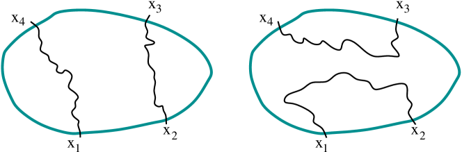
Figure 30: Arch configurations for four SLE processes in an arbitrary domain.

To present the simplest non trivial example [14] we consider critical models in the upper half plane $\mathbb{H}$ with boundary conditions changing at $4$ points so that there is two interfaces each joining a pair of points. See Fig.30. By conformal invariance we may normalize the points so that $X_{1}=0$, $X_{2}=x$, $X_{3}=1$ and $X_{4}=\infty$ with $0<x<1$. There are two distinct topological configurations and therefore two pure partition functions, which by construction may be written as correlation functions

$$Z(x)=\langle\psi(\infty)\psi(1)\psi(x)\psi(0)\rangle_{\mathbb{H}}$$

Their behavior when points are fused are governed by CFT fusion rules. As a consequence, $Z(x)$ behave either as $x^{\frac{\kappa-6}{\kappa}}$ or as $x^{\frac{2}{\kappa}}$ as $x\to 0$. The pure partition functions $Z_{I}$ and $Z_{II}$ are specified by the way they behave when points are fused together:

$$Z_{I}(x) = x^{\frac{\kappa-6}{\kappa}}\times[1+\cdots],\quad~{}~{}~{}~{}~{}~{}~{}~{}~{}~{}~{}~{}{\rm as}\ x\to 0$$

$$= (1-x)^{\frac{2}{\kappa}}\times[{\rm const.}+\cdots],\quad~{}{\rm as}\ x\to 1$$

and $Z_{II}(x)=Z_{I}(1-x)$. The function $Z_{I}$ turns out to be the pure partition function for configurations in which the curves join the pairs $[0x]$ and $[1\infty]$ while $Z_{II}$ corresponds to the configurations $[x1]$ and $[\infty 0]$. The rationale behind these conditions consists in imposing that the pure partition function possesses the leading singularity, with exponent $(6-\kappa)/\kappa$, when $x$ is approaching the point allowed by the configuration but has sub-leading singularity, with exponent $2/\kappa$, when $x$ is approaching the point forbidden by the configuration. This set of conditions uniquely determines the functions $Z_{I}$ and $Z_{II}$. These follows from CFT rules but may also be checked by explicitly solving the differential equation that these functions satisfy. Writing $Z(x)=x^{2/\kappa}(1-x)^{2/\kappa}\;G(x)$ yields,

$$\kappa^{2}x(1-x)G^{\prime\prime}(x)+8\kappa(1-2x)G^{\prime}(x)-4(12-\kappa)G(x)=0$$

so that $G(x)$ is an hypergeometric function and

$$Z_{II}(x)={\rm const.}x^{2/\kappa}(1-x)^{2/\kappa}\;F(\frac{4}{\kappa},\frac{12-\kappa}{\kappa};\frac{8}{\kappa}|x)$$

with the constant chosen to normalize $Z_{I}$ as above. Using this explicit formula one may verify that $Z_{I}(x)$ is effectively a positive number for any $x\in[0;1]$ so it has all expected properties to be a pure partition function. For $\kappa=4$, $Z_{I}(x)=\sqrt{(1-x)/x}$ and for $\kappa=2$, $Z_{I}(x)=(1-x^{2})/x^{2}$.

A generic partition function $Z$ is a weighted sum of the pure partition functions: $Z(x)=p_{I}Z_{I}(x)+p_{II}Z_{II}(x)$ with $p_{I}$ and $p_{II}$ positive. The probability of occurrence of topological configurations $I$ and $II$ are then:

$${\bf P}[{\rm config}_{I}]=p_{I}Z_{I}(x)/Z(x)\quad,\quad{\bf P}[{\rm config}_{II}]=p_{II}Z_{II}(x)/Z(x)$$

— Ising spin clusters correspond to $\kappa=3$. The boundary changing operator $\psi$ has dimension $1/2$ and may thus be identified with a fermion on the boundary. However the pure partition functions do not correspond to the free fermion conformal block. By solving the differential equation with the appropriate boundary condition we get:

$$Z_{I}(x)_{\rm spin\ Ising}=\mathrm{const.}\,\frac{1-x+x^{2}}{x(1-x)}\int_{x}^{1}dy\frac{(y(1-y))^{2/3}}{(1-y+y^{2})^{2}}$$

The total partition function $Z_{I}(x)+Z_{I}(1-x)$ is proportional to $\frac{1-x+x^{2}}{x(1-x)}$, which is the free fermion result. Hence, the Ising configuration probabilities, which are nothing but crossing formula for spin clusters, are:

$${\bf P}[{\rm config}_{I}]_{\rm spin\ Ising}=\int_{x}^{1}dy\frac{(y(1-y))^{2/3}}{(1-y+y^{2})^{2}}\;\Big{/}\int_{0}^{1}dy\frac{(y(1-y))^{2/3}}{(1-y+y^{2})^{2}}$$

— FK Ising clusters correspond to $\kappa=16/3$. The operator $\psi$ has then dimension $1/16$. The pure partition function are given by:

$$Z_{I}(x)_{\rm FK\ Ising}=\frac{(1-x)^{3/8}}{x^{1/8}(1+\sqrt{x})^{1/2}}$$

and the crossing probabilities by:

$${\bf P}[{\rm config}_{I}]_{\rm FK\ Ising}=\frac{\sqrt{(1-x)+(1-x)^{3/2}}}{\sqrt{x+x^{3/2}}+\sqrt{(1-x)+(1-x)^{3/2}}}$$

— The other critical random cluster (or Potts) models with $0\leq Q\leq 4$ have $Q=4\cos^{2}\big{(}\frac{4\pi}{\kappa}\big{)}$, $4\leq\kappa\leq 8$, and it is straightforward to obtain explicit crossing formulas involving only hypergeometric functions. The case $\kappa=6$ reproduces Cardy’s crossing formula for percolation.

5.6 Miscellaneous

Another approach to the CFT/SLE correspondence has been proposed in [62, 63]. It uses the restriction properties to be discussed in Section 6.2. The restriction property holds for SLE only for $\kappa=8/3$, which corresponds to the central charge $c=0$. However, the restriction property can be recovered for $\kappa<8/3$ be dressing the SLE curves with Brownian bubbles associated to the Brownian loop soup to be described in Section 6.4. This approach was later generalized in [43] to identify the CFT stress-tensor within the SLE framework.

Generalizations of SLEs to a larger class of CFTs, with central charges bigger than one and with more degrees of freedom than those described above, have of course been considered. These include supersymmetric [112, 102] or logarithmic [113, 106] generalizations. The cases corresponding to CFT with Lie-group symmetry, described by the Wess-Zumino-Witten models, have been discussed in ref.[24]. The outcome of these studies is that for describing interfaces in CFT with higher central charges one needs to add extra degrees of freedom along the interfaces but as a geometrical objects, ie. as curves, these interfaces are still described by the standard SLE with some effective parameter $\kappa$ corresponding to some effective central charge less than one. This had to be expected because Schramm’s argument implies that conformally invariant curves have to be described by the standard SLEs.

SLEs in different topologies than that of a disc have been considered: refs.[45, 142, 11] discussed SLEs in annuli and ref.[15, 16, 17] defined SLEs in multiply connected domains. These explicit constructions show that the moduli parameters of the domains change in time while the SLE curves are growing. This is clear in the case of the annuli in which case the only moduli is the ratio of radii of the inner and outer circles. An annulus cutted along a piece of curve grown say from the outer circle is topologically equivalent to another annulus but with different ratio of radii. In the annulus case the SLE process stops at the instant the curve touches the inner circle. An attempt to formalize SLEs as motions in the moduli spaces of Riemann surfaces has been written in [64].

6 SLE delicatessen

This Section aims at presenting some of the remarkable – and quite beautiful – structures and properties of conformally invariant curves or hulls. Some of them are pure SLE properties, others involve extra conformally invariant measures on hulls. The first is a locality property of SLE₆ which is inherited from the locality property of percolation. The second refers to the notion of restriction measures which concerns measures on hulls such that the measures for hulls on a domain $\mathbb{D}$ conditioned not to touch some fixed hull $\mathbb{A}$ is identical to the measure for hulls on $\mathbb{D}\setminus\mathbb{A}$. This properties holds for SLE only for $\kappa=8/3$. It also holds for Brownian excursion and this provides a way to prove [93, 97] Mandelbrot’s conjecture that the fractal dimension of the exterior perimeter of Brownian excursion is $4/3$. We also presents Duplantier’s predictions concerning the fractal spectrum of harmonic measures of conformally invariant hulls. To prove this prediction is one of the remaining big challenge of the SLE project. Finally we describe the Brownian loop soup which was introduced in ref.[98] in connection with restriction measures.

6.1 Locality of $SLE_{6}$

In percolation there is no interaction in the sense that the color of the sites are chosen with given probability independently to those of the other sites of the system. This implies that, on the lattice, the exploration process used to recursively construct an interface is defined by local rules. In the continuum, and at criticality, this translates into the locality property of SLE₆ which signifies that its hull does not feel the boundary of the domain, or portion the domain, before it visits it.

To be more concrete consider chordal SLE in the upper half plane $\mathbb{H}$. Let us deform it by removing a hull $\mathbb{A}$. Let $\phi_{\mathbb{A}}$ be the map uniformizing $\mathbb{H}\setminus\mathbb{A}$ onto $\mathbb{H}$ normalized by $\phi_{\mathbb{A}}(0)=0$, $\phi_{\mathbb{A}}(\infty)=\infty$ and $\phi_{\mathbb{A}}^{\prime}(\infty)=1$. We want to compare SLE in $\mathbb{H}$ and in $\mathbb{H}\setminus\mathbb{A}$. By conformal transport, this amounts to compare the SLE trace $\gamma_{[0,t[}$ in $\mathbb{H}$ and its image $\phi_{\mathbb{A}}(\gamma_{[0,t[})$, again in $\mathbb{H}$, with the hope of proving that they have identical law,

$$\gamma_{[0,t[}\ \equiv_{\rm in~{}law}\phi_{\mathbb{A}}(\gamma_{[0,t[})$$ (46)

up to a possible random time change. This turns out to be true only at $\kappa=6$.

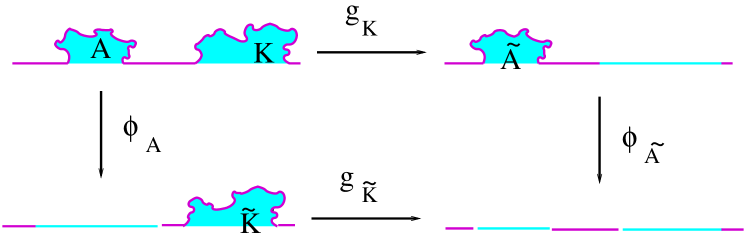
Figure 31: The commutative diagram associated to the two alternative ways of uniformizing the complement of two hulls. It codes for the relation $\phi_{\tilde{A}}\circ g_{K}=g_{\tilde{K}}\circ\phi_{A}$.

This proof is an interesting exercise [90, 101]. It is based on the fact that we can uniformize the complement of the union of the hull and of the trace in two different ways: either erasing first the trace $\gamma_{[0,t[}$ using the SLE Loewner map $g_{t}$ and then the modified hull $\mathbb{A}_{t}$ using a map $\phi_{\mathbb{A}_{t}}$, or erasing first the hull $\mathbb{A}$ using $\phi_{\mathbb{A}}$ and then the modified curve $\phi_{A}(\gamma_{[0,t[})$ using another Loewner map $k_{t}$. See Fig.31. This translates into the commutative diagram [90, 97]:

$$\phi_{\mathbb{A}_{t}}\circ g_{t}=k_{t}\circ\phi_{\mathbb{A}}.$$ (47)

Here $\phi_{\mathbb{A}_{t}}$ is normalized the same way as $\phi_{\mathbb{A}}$. Since $k_{t}$ is a map (properly normalized) uniformizing of the complement of a curve, it satisfies the Loewner equation $\partial_{t}k_{t}(z)=a_{t}/(z-W_{t})$. The source $W_{t}$ is the image of the modified curve, $k_{t}(\phi_{\mathbb{A}}(\gamma_{t}))$, which is equal to $W_{t}=\phi_{\mathbb{A}_{t}}(\xi_{t})$ thanks to the commutative diagram. The evolution equation for $\phi_{\mathbb{A}_{t}}$ directly follows from the commutative diagram:

$$\partial_{t}\phi_{\mathbb{A}_{t}}(w)=\frac{a_{t}}{\phi_{\mathbb{A}_{t}}(w)-W_{t}}-\frac{2\phi_{\mathbb{A}_{t}}^{\prime}(\xi_{t})}{w-\xi_{t}}$$

The map $\phi_{\mathbb{A}_{t}}$ is regular at point $\xi_{t}$ because the modified hull $\mathbb{A}_{t}$ is away from it. Demanding that its time derivative is also regular at $\xi_{t}$ fixes $a_{t}=2\phi_{\mathbb{A}_{t}}^{\prime}(\xi_{t})^{2}$. The limit is then $\partial_{t}\phi_{\mathbb{A}_{t}}(\xi_{t})=-3\phi_{\mathbb{A}_{t}}^{\prime\prime}(\xi_{t})$.

To prove locality we have to prove that $k_{t}$ defines a SLE process up to a random time change which amounts to prove that $W_{t}$ is a Brownian motion up to the random time change specified by $a_{t}$. Itô’s formula gives $dW_{t}=\partial_{t}\phi_{\mathbb{A}_{t}}(\xi_{t})dt+\phi_{\mathbb{A}_{t}}^{\prime}(\xi_{t})d\xi_{t}+\frac{\kappa}{2}\phi_{\mathbb{A}_{t}}^{\prime\prime}(\xi_{t})dt$. Thanks to the previous evaluation of $\partial_{t}\phi_{\mathbb{A}_{t}}(\xi_{t})$ the first and last terms are similar so that:

$$dW_{t}=(\frac{\kappa-6}{2})\phi_{\mathbb{A}_{t}}^{\prime\prime}(\xi_{t})dt+\phi_{\mathbb{A}_{t}}^{\prime}(\xi_{t})d\xi_{t}$$

The drift term vanishes for $\kappa=6$ so that $W_{t(s)}$ is a Brownian motion up to the change $ds=\phi_{\mathbb{A}_{t}}^{\prime}(\xi_{t})^{2}dt$. This proves locality at $\kappa=6$.

6.2 Restrictions

Restriction measures [97] are measures for conformally invariant random hulls with the property that the law of the hulls in a domain $\mathbb{D}$ conditioned not to visit a fixed hull $\mathbb{A}$ is identical to that of the random hulls in the domain $\mathbb{D}\setminus\mathbb{A}$ with the hull removed, see Fig.32.

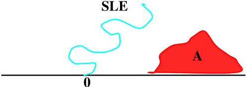
Figure 32: A SLE curve growing in the upper half plane minus a hull $\mathbb{A}$ or conditioned not to touch this hull.

These laws of been studied and classified in [97]: there is a one parameter family of such measures. By conformal invariance it is enough to look at them for hulls in the upper half plane. Let $\mathbb{K}\subset\mathbb{H}$ be the random hulls. Their law is characterized by the set of probabilities ${\bf P}[\mathbb{K}\cap\mathbb{A}=\emptyset]$ that they do not intersect fixed hulls $\mathbb{A}$. As proved in [97], the restriction property imposes that these probabilities are of the following form:

$${\bf P}[\mathbb{K}\cap\mathbb{A}=\emptyset]=\phi_{\mathbb{A}}^{\prime}(0)^{\alpha},\quad{\rm for}\ \mathbb{K}\subset\mathbb{H}$$ (48)

with $\phi_{\mathbb{A}}$ the conformal map uniformizing $\mathbb{H}\setminus\mathbb{A}$ back onto $\mathbb{H}$, normalized by $\phi_{\mathbb{A}}(0)=0$, $\phi_{\mathbb{A}}(\infty)=\infty$ and $\phi_{\mathbb{A}}^{\prime}(\infty)=1$. The exponent $\alpha$ specifies the measure. It has to be bigger than $5/8$. The greater is $\alpha$ the thicker are the hulls: $\alpha=5/8$ corresponds to random simple curves – actually to SLE_8/3 as we shall see below.

It is an instructive exercise to check that the measures (48) indeed satisfy the restriction property, ie. the law in $\mathbb{H}$ of the hulls $\mathbb{K}$ conditioned not to touch a given hull $\mathbb{A}$ is identical to the law in $\mathbb{H}\setminus\mathbb{A}$:

$$\mathbb{K}\subset\mathbb{H}\ \Big{|}(\mathbb{K}\cap\mathbb{A}=\emptyset)\equiv_{\rm in~{}law}\mathbb{K}\subset\mathbb{H}\setminus\mathbb{A}$$

To check it we pick another arbitrary hulls $\mathbb{B}$ disjoint from $\mathbb{A}$, we look at the probabilities that the hulls viewed as conditioned hulls in $\mathbb{H}$ or as hulls in $\mathbb{H}\setminus\mathbb{A}$ do not intersect $\mathbb{B}$ and we prove that:

$${\bf P}_{\rm in~{}\mathbb{H}}[\mathbb{K}\cap\mathbb{B}=\emptyset\ \Big{|}\mathbb{K}\cap\mathbb{A}=\emptyset]={\bf P}_{\rm in~{}\mathbb{H}\setminus\mathbb{A}}[\mathbb{K}\cap\mathbb{B}=\emptyset]$$

The conditioned probability in the left hand side is the ratio of the probability that $\mathbb{K}$ does not touch $\mathbb{A}\cup\mathbb{B}$ by the probability that it does not touch $\mathbb{A}$, so it is $\phi_{\mathbb{A}\cup\mathbb{B}}^{\prime}(0)^{\alpha}/\phi_{\mathbb{A}}^{\prime}(0)^{\alpha}$ where $\phi_{\mathbb{A}\cup\mathbb{B}}$ and $\phi_{\mathbb{A}}$ are the respective uniformizing conformal maps properly normalized. The complement of the union $\mathbb{A}\cup\mathbb{B}$ can be uniformized in two steps: first erasing the hull $\mathbb{A}$ using $\phi_{\mathbb{A}}$ and then erasing the image $\hat{\mathbb{B}}\equiv\phi_{\mathbb{A}}(\mathbb{B})$ of the remaining hull using the appropriate normalized conformal map $\phi_{\hat{\mathbb{B}}}$. This yields $\phi_{\mathbb{A}\cup\mathbb{B}}=\phi_{\hat{\mathbb{B}}}\circ\phi_{\mathbb{A}}$ so that:

$${\bf P}_{\rm in~{}\mathbb{H}}[\mathbb{K}\cap\mathbb{B}=\emptyset\ \Big{|}\mathbb{K}\cap\mathbb{A}=\emptyset]=\phi_{\hat{\mathbb{B}}}^{\prime}(0)^{\alpha},\quad\hat{\mathbb{B}}=\phi_{\mathbb{A}}(\mathbb{B})$$

This is also ${\bf P}_{\rm in~{}\mathbb{H}\setminus\mathbb{A}}[\mathbb{K}\cap\mathbb{B}=\emptyset]$ because the law in $\mathbb{H}\setminus\mathbb{A}$ is defined from that in the upper half plane by conformal transport.

As explained in [136], there exists a nice interplay between SLE$(\kappa,\rho)$ and restriction measures. Indeed an SLE$(\kappa,\rho)$ can be viewed as an SLE_κ conditioned not to touch a restriction sample with exponent $\alpha=\rho(\rho+4-\kappa)/4\kappa$. Furthermore, an SLE$(\kappa,\rho)$ conditioned not touch a restriction sample with exponent $\alpha$ is another SLE$(\kappa,\bar{\rho})$ with $2\bar{\rho}=\kappa-4+\sqrt{16\kappa\alpha+(2\rho+4-\kappa)^{2}}$. A relation between reflected Brownian motions and restriction measures is given in [97].

6.2.1 The restriction property of SLE_8/3

Here we present the arguments [97] showing that chordal SLE_8/3 satisfies the restriction property with $\alpha=5/8$. Note that this value is that of the dimension of the operator $\psi_{1;2}$ creating the SLE trace: $h_{1;2}=5/8$ at $\kappa=8/3$. So we have to compute the probability that the SLE_8/3 curve does not touch a bounded hull $\mathbb{A}$ away from the origin. If it is equal to $\phi_{\mathbb{A}}^{\prime}(0)^{5/8}$, then, by the usual Markov and independent increment properties of SLE, the process (up to the hitting time of $\mathbb{A}$),

$$M_{t}(\mathbb{A})=\phi_{\mathbb{A}_{t}}^{\prime}(\xi_{t})^{5/8},\quad\kappa=8/3$$

is a martingale with $\mathbb{A}_{t}\equiv g_{t}(\mathbb{A})$ with $g_{t}$ the SLE Loewner map and $\phi_{\mathbb{A}_{t}}$ the corresponding uniformizing map fixing $0$ and $\infty$ with $\phi_{\mathbb{A}_{t}}^{\prime}(\infty)=1$. We shall prove it a bit later.

Reciprocally, if $M_{t}(\mathbb{A})$ is a martingale then

$${\bf P}[\gamma_{[0,\infty[}\cap\mathbb{A}=\emptyset]=\phi_{\mathbb{A}}^{\prime}(0)^{5/8},\quad\kappa=8/3$$

Indeed, choose a very large semi circle ${\mathcal{C}}_{R}$ of radius $R$ in $\mathbb{H}$ centered at the origin. Let $\tau_{R}$ be the first time when the trace touches either $\mathbb{A}$ or ${\mathcal{C}}_{R}$. Then $\tau_{R}$ is a stopping time and we claim that $\phi_{\hat{\mathbb{A}}_{\tau_{R}}}^{\prime}(\xi_{\tau_{R}})$ is $0$ if the SLE hull hits $\mathbb{A}$ at $\tau_{R}$ and goes to $1$ for large $R$ if the SLE hull hits ${\mathcal{C}}_{R}$ at $\tau_{R}$. Indeed, when the hull approaches $\mathbb{A}$, one or more points on $\hat{\mathbb{A}}_{t}$ approach $\xi_{t}$, and at the hitting time, a bounded connected component is swallowing $\xi_{t}$ indicating that the derivative has to vanish there. On the other hand, if ${\mathcal{C}}_{R}$ is hit first, then $\hat{\mathbb{A}}_{\tau_{R}}$ is dwarfed so that $\phi_{\hat{\mathbb{A}}_{\tau_{R}}}$ is close to the identity map away from $\hat{\mathbb{A}}_{\tau_{R}}$ and in particular at the point $\xi_{\tau_{R}}$. (The normalization of the conformal maps are crucial for proving these statements.) Hence, the martingale $\phi_{\hat{\mathbb{A}}_{t}}^{\prime}(\xi_{t})^{5/8}$, at $t=\tau_{R}$, is $0$ if $\mathbb{A}$ is hit before ${\mathcal{C}}_{R}$ and close to $1$ if the opposite is true. But the expectation of a martingale is time independent, so that the probability that the trace does not hit $\mathbb{A}$ is $\phi_{\mathbb{A}}^{\prime}(0)^{5/8}$. This shows that SLE_8/3 satisfies the restriction property.

The proof that $M_{t}(\mathbb{A})$ is a martingale is similar to the proof of the locality property [97]. It is again based on the commutative diagram (47): $\phi_{\mathbb{A}_{t}}\circ g_{t}=k_{t}\circ\phi_{\mathbb{A}}$. Let us recall that $k_{t}$ is the map uniformizing the complement of the image curve $\phi_{\mathbb{A}}(\gamma_{[0,t[})$. It satisfies the Loewner equation $\partial_{t}k_{t}(z)=a_{t}/(z-W_{t})$ with $W_{t}=\phi_{\mathbb{A}_{t}}(\xi_{t})$ and $a_{t}=2\phi_{\mathbb{A}_{t}}^{\prime}(\xi_{t})^{2}$. The evolution equation for $\phi_{\mathbb{A}_{t}}$ follows from the commutative diagram:

$$\partial_{t}\phi_{\mathbb{A}_{t}}(w)=\frac{2\phi_{\mathbb{A}_{t}}^{\prime}(\xi_{t})^{2}}{\phi_{\mathbb{A}_{t}}(w)-W_{t}}-\frac{2\phi_{\mathbb{A}_{t}}^{\prime}(\xi_{t})}{w-\xi_{t}}$$

The map $\phi_{\mathbb{A}_{t}}$ is regular at point $\xi_{t}$ because the modified hull $\mathbb{A}_{t}$ is away from $\xi_{t}$. Taking the derivative with respect to $w$ and then the limit $w\to\xi_{t}$ gives:

$$\partial_{t}\phi_{\mathbb{A}_{t}}^{\prime}(\xi_{t})=\phi_{\mathbb{A}_{t}}^{\prime\prime}(\xi_{t})^{2}/2\phi_{\mathbb{A}_{t}}^{\prime}(\xi_{t})-4\phi_{\mathbb{A}_{t}}^{\prime\prime\prime}(\xi_{t})/3$$

This allows to compute the Itô derivative of $\phi_{\mathbb{A}_{t}}^{\prime}(\xi_{t})^{\alpha}$ :

$$d\phi_{\mathbb{A}_{t}}^{\prime}(\xi_{t})^{\alpha}=\alpha\phi_{\mathbb{A}_{t}}^{\prime}(\xi_{t})^{\alpha}[\,(3\kappa-8)\frac{\phi_{\mathbb{A}_{t}}^{\prime\prime\prime}(\xi_{t})}{6\phi_{\mathbb{A}_{t}}^{\prime}(\xi_{t})}+(\kappa\alpha-\kappa+1)\frac{\phi_{\mathbb{A}_{t}}^{\prime\prime}(\xi_{t})^{2}}{2\phi_{\mathbb{A}_{t}}^{\prime}(\xi_{t})^{2}}\,]dt+[\cdots]d\xi_{t}$$

The drift term vanishes for $\kappa=8/3$ and $\alpha=5/8$, which proves that $M_{t}(\mathbb{A})$ is a local martingale.

For $\kappa\not=8/3$, the process $\phi_{\mathbb{A}_{t}}^{\prime}(\xi_{t})^{5/8}$ is not a martingale but the following one [97],

$$\phi_{\mathbb{A}_{t}}^{\prime}(\xi_{t})^{h_{1;2}}\,\exp-\frac{c}{6}\int_{0}^{t}ds\,(S\cdot\phi_{\mathbb{A}_{s}})(\xi_{s}),$$ (49)

with $S\cdot\phi$ the Schwarzian derivative of $\phi$, $c=(6-\kappa)(8\kappa-3)/2\kappa$ the central charge and $h_{1;2}=(6-\kappa)/2\kappa$, is a martingale. The fact that it is a martingale can be proved as above using the commutative diagram [97] or using the algebraic formulation of SLE [9]. The extra term is present for non zero central charge because this martingale codes the way SLEs react to deformations of the domain. Similar formula exist for other SLEs, eg. for radial SLE [97, 10].

6.2.2 The Brownian exterior perimeter

Naively, a two dimensional Brownian excursion $\mathfrak{B}_{t}$ from say $0$ to $\infty$ is a Brownian walk started at the origin conditioned to remain in the upper half plane and to escape to $\infty$. This has to be made more precise since such events happen with probability zero! The cleaner mathematical definition consists in setting $\mathfrak{B}_{t}=B_{t}+iY_{t}$ with $B_{t}$ a standard Brownian motion and $Y_{t}$ a Bessel process. Instead, we choose the most physical one, and we consider a Brownian walk started at point $i\epsilon$ ($\epsilon>0$) conditioned to escape first through line $i\Lambda+\mathbb{R}$ $(\Lambda>0)$ before touching the real axis $\mathbb{R}$. This happens with probability $\epsilon/\Lambda$. We then take the limit $\epsilon\to 0$ and $\Lambda\to\infty$ and we look at events for which the conditioned probabilities are finite in this limit.

Let us show that Brownian excursion satisfies the restriction property. Let $\mathbb{A}$ be a hull in the upper half plane. We have to compute the probability ${\bf P}(\mathfrak{B}_{]0,\infty[}\cap\mathbb{A}=\emptyset)$ that the Brownian excursion does not touch this hull. By the above definition, this is the probability for a 2d Brownian motion started at $i\epsilon$ not to touch $\mathbb{A}$ conditioned to escape first on $i\Lambda+\mathbb{R}$. So it is the ratio of the probability that the 2d Brownian motion started at $i\epsilon$ does not touch $\mathbb{A}$ and escapes through $i\Lambda+\mathbb{R}$ by the probability – equal to $\epsilon/\Lambda$ – that it escapes through $i\Lambda+\mathbb{R}$. To compute it we use conformal invariance of the 2d Brownian motion. Let $\phi_{\mathbb{A}}$ be the conformal map uniformizing $\mathbb{H}\setminus\mathbb{A}$ onto $\mathbb{H}$ fixing $0$ and $\infty$ and such that $\phi_{\mathbb{A}}^{\prime}(\infty)=1$. The image of the starting point under this map is $\phi_{\mathbb{A}}(i\epsilon)\simeq i\epsilon\phi_{\mathbb{A}}^{\prime}(0)$ for $\epsilon\ll 1$ and the straight line $i\Lambda+\mathbb{R}$ at infinity is mapped under a line at infinity slightly waving around $i\Lambda+\mathbb{R}$ since $\phi_{\mathbb{A}}(\infty)=\infty$ and $\phi_{\mathbb{A}}^{\prime}(\infty)=1$. Thus, the probability that the 2d Brownian motion started at $i\epsilon$ does not touch $\mathbb{A}$ and escapes through $i\Lambda+\mathbb{R}$ is, by conformal invariance, the probability that the 2d Brownian motion started at $i\epsilon\phi_{\mathbb{A}}^{\prime}(0)$ escapes through the line $i\Lambda+\mathbb{R}$. This is equal to $\epsilon\phi_{\mathbb{A}}^{\prime}(0)/\Lambda$. Finally, the probability that the Brownian excursion does not touch the hull $\mathbb{A}$ is:

$${\bf P}[\mathfrak{B}_{]0,\infty[}\cap\mathbb{A}=\emptyset]=\frac{\epsilon\phi_{\mathbb{A}}^{\prime}(0)/\Lambda}{\epsilon/\Lambda}=\phi_{\mathbb{A}}^{\prime}(0)$$

Since this is valid for any hull, it proves that Brownian excursions in the upper half plane – more precisely hulls obtained by filling the domain surrounded by the Brownian excursions – form a restriction measure with exponent $1$.

We can now compare Brownian excursions and self avoiding walks. Consider $5$ independent Brownian excursions. By construction they form a restriction measure with exponent $5$ – that is the probability that none of these excursions hit a hull $\mathbb{A}$ is $\phi_{\mathbb{A}}^{\prime}(0)^{5}$. Similarly $8$ independent SLE_8/3 – ie. $8$ self avoiding walks – also form a restriction measure with exponent $5$ since each of them form a restriction measure with exponent $5/8$. As a consequence we have an identification of the distribution of these hulls [97]:

$$5\ {\rm Brownian~{}excursions}\equiv_{\rm in~{}law}8\ {\rm SLE}_{8/3}$$

This identification yields to a poor (wo)man argument for Mandelbrot’s conjecture on the fractal dimension of the Brownian exterior perimeter. Indeed, the exterior perimeter of the hull formed by filling the space surrounded by the five Brownian excursions is locally the exterior perimeter of one of these excursions. Similarly, the exterior perimeter of the hull formed by the eight SLE_8/3 is locally one of these SLEs since they are simple curve. Thus the fractal dimension of the exterior perimeter of a Brownian excursion equals that of $SLE_{8/3}$. Namely

$${\rm dim.~{}Brownian~{}perimeter}=d_{8/3}=4/3$$

The mathematical proof of this statement has been one of the main achievement of the SLE project [93, 97]. It was originally based on the observation that the outer boundary of Brownian excursion is the same as that of SLE₆. SLE also gives the dimension $3/4$, which is the dimension of the set of double points in SLE₆, for the set of cut points of Brownian paths.

6.3 Multifractal harmonic measure

6.3.1 Harmonic measure

The harmonic measure of a planar domain $\mathbb{U}$ is linked to the hitting probability distribution of a random walker when she/he escapes from $\mathbb{U}$. To be more precise let us consider a planar domain $\mathbb{U}$ with the topology of a disc and point $z_{0}$ in the interior of $\mathbb{U}$. Consider a two dimensional Brownian motion $X_{t}$ started at point $z_{0}$ and stopped at the first instant $\tau_{\mathbb{U}}$ it exits from $\mathbb{U}$. Then the harmonic measure $\mu_{z_{0}}$, which is a measure on the boundary, is the probability that the Brownian motion escapes from the domain through a subset of its boundary:

$$\mu_{z_{0}}({F})\equiv{\bf P}_{z_{0}}[X_{\tau_{\mathbb{U}}}\in{F}],\quad{F}\subset\partial\mathbb{U}$$

By construction, it is harmonic as a function of the starting position $z_{0}$ with boundary condition $\mu_{z_{0}}({F})=1$ if $z_{0}\in F$ and $0$ if $z_{0}$ is approaching the complement of $F$ on $\partial\mathbb{U}$. The harmonic measure has many applications to generalized Dirichlet problems [110].

The simplest example is for $\mathbb{U}$ the unit disc and $z_{0}$ the origin. The hitting distribution is then uniform on the unit circle so that in this case $d\mu_{0}=d\theta/2\pi$ with $\theta\in[0,2\pi[$ the angle parameterizing the unit circle. This gives a way to compute the harmonic measure (for sufficiently regular boundary). Let $w$ be a conformal map uniformizing $\mathbb{U}$ onto the unit disc with $w(z_{0})=0$, then $\mu_{z_{0}}(F)=\int_{F}|dw(z)|$ by conformal invariance of the two dimensional Brownian.

The harmonic measure is sensible to the local geometry of the boundary and linked to the behavior of the (derivative of the) uniformizing map close the boundary. Consider for instance the wedge $\mathcal{W}_{\theta}\equiv\{z\in\mathbb{C},0<{\rm arg}\,z<\theta\}$ of angle $\theta$. A uniformizing map of $\mathcal{W}_{\theta}$ onto the unit disc is $w(z)=\frac{z^{\pi/\theta}+i}{z^{\pi/\theta}-i}$. For $z$ at a distance $\varepsilon$ from the boundary $\varepsilon\,|w^{\prime}(z)|$ behaves as $\varepsilon^{\pi/\theta}$. The harmonic measure $\mu_{*}(\partial W_{\theta}\cap B_{\varepsilon})$ of the portion of the boundary of the wedge contained in the ball of size $\varepsilon$ centered at the tip of the wedge scales the same way as $\varepsilon^{\pi/\theta}$.

We shall be interested in cases in which a portion of the boundary of the domain is the boundary of critical clusters so that it looks locally as a SLE curve with parameter $\kappa<4$. We may for instance have in mind a domain minus SLE hulls (run during sufficiently enough time).

6.3.2 Multifractal spectrum

The multifractal spectrum of harmonic measures of boundaries of critical clusters has been predicted by B. Duplantier in a serie of papers [55, 56, 57, 58] using arguments based on applications of 2D gravity and of the KPZ formula [82] for gravitationally dressed dimensions. See the reviews [59, 60]. It is defined by considering the expectation values of moments of the harmonic measure of the boundary curve. More precisely, let us define

$$\mathcal{Z}_{n}={\bf E}\left[{\sum_{B_{\varepsilon}}[\mu_{*}(\gamma\cap B_{\varepsilon})]^{n}}\right]$$

where the sum is over a set of boxes $B_{\varepsilon}$ of size $\varepsilon$ covering the boundary curve $\gamma$ and $\mu_{*}$ is the harmonic measure. For $n=0$ the sum is simply the number of boxes needed to cover the curve. So by definition of the fractal dimension it scales as $\mathcal{Z}_{0}\approx\varepsilon^{-d_{\kappa}}$. For $n=1$ the sum reproduces the total harmonic measure $\mu_{*}(\gamma)$ of the curve which we assumed to be normalized to one, so that $\mathcal{Z}_{1}=1$. More generally, scaling behavior of $\mathcal{Z}_{n}$ defines the multifractal exponents $\tau_{n}$ via $\mathcal{Z}_{n}\approx\varepsilon^{\tau_{n}}$. Duplantier’s prediction is:

$$\tau_{n}=\frac{n-1}{2}+\frac{\kappa+4}{16\kappa}\,\big{[}{\sqrt{16n\kappa+(\kappa-4)^{2}}-(\kappa+4)}\big{]}$$ (50)

As it should be, it is invariant under the duality $\kappa\to 16/\kappa$ and $-\tau_{0}$ reduces to the fractal dimension of the exterior perimeter. The harmonic measure is only sensible to the exterior perimeter, so we shall choose the branch $\kappa<4$.

By standard multifractal arguments [104, 71], the multifractal dimensions $f_{\alpha}$ are obtained from $\tau_{n}$ by a Legendre transform. Let us recall it. Consider the set $\mathcal{C}_{\alpha}$ of points in which the harmonic measure, evaluated on a ball $B_{\varepsilon}$ intersecting the curve at a point of $\mathcal{C}_{\alpha}$, scales as $\varepsilon^{\alpha}$. By definition, $f_{\alpha}$ is the fractal dimension of $\mathcal{C}_{\alpha}$. We may replace the sum defining $\mathcal{Z}_{n}$ by a sum over all boxes of sizes $\varepsilon$ covering the full domain – there are of order $\approx\varepsilon^{-2}$ of such boxes – and over the sets $\mathcal{C}_{\alpha}$ weighted by the probability that they intersect one of these balls – this probability scales as $\varepsilon^{2-f_{\alpha}}$ by definition of the fractal dimension. Over the set $\mathcal{C}_{\alpha}$ the $n^{\rm th}$ moment of the harmonic measure behaves as $\varepsilon^{n\alpha}$. Hence, $\mathcal{Z}_{n}$ scales as $\int d\nu_{\alpha}\,\varepsilon^{n\alpha-f_{\alpha}}$. Saddle point approximation valid for $\varepsilon\to 0$ gives

$$\tau_{n}=n\alpha-f_{\alpha},\quad df_{\alpha}/d\alpha=n$$

This is a Legendre transform so that $f_{\alpha}$ may be computed by inverting it: $f_{\alpha}=\tau_{n}-n\alpha$ with $d\tau_{n}/dn=\alpha$. The result is:

$$f_{\alpha}=\frac{(\kappa+4)^{2}}{16\kappa}\,\frac{3\alpha-2}{2\alpha-1}-\frac{(\kappa-4)^{2}}{16\kappa}\,\alpha$$ (51)

with $\alpha\in]1/2,+\infty[$. It satisfies Makarov’s theorem [103] which states that $\tau^{\prime}(1)=1$ or alternatively $f_{\alpha=1}=1$. By construction, the maximum of $f_{\alpha}$ is for $df_{\alpha}/d\alpha=0$ so that $f_{\alpha}|_{\rm max}=-\tau_{0}$ is the fractal dimension.

The sets $\mathcal{C}_{\alpha}$ are sets of points in which the exterior perimeter has locally the geometry of a wedge with angle $\pi/\alpha$, so that the harmonic measure scales locally as $\varepsilon^{\alpha}$. The typical geometry is a wedge of angle $\theta^{*}=\pi/\alpha^{*}=\pi(1-\kappa/4)$, we choose the branch $\kappa<4$. It corresponds to the value $\alpha^{*}$ at which $f_{\alpha}$ reaches its maximum. The minimum value $\alpha_{\rm min}=1/2$ corresponds to the maximum angle $2\pi$ so that the curve looks locally like a needle. This minimum value governs the large $n$ behavior of the multifractal exponents $\tau_{n}\simeq n/2$ for $n\gg 1$. Large values of $\alpha$ correspond to small angles and therefore to local fjords, and $f_{\alpha}\simeq n^{*}\alpha$ asymptotically for $\alpha\gg 1$. They govern the behavior of the lowest moments as $n\searrow n^{*}$. Moments of order less that $n^{*}$ do not exist.

No mathematically complete proof of Duplantier’s predictions have yet been published. Besides original Duplantier’s arguments there are however hints for these formulas based on conformal field theory. The first hint comes by observing [7] that KPZ formulas of 2D gravity [82] naturally arise in SLE because they are linked to operator product expansion with the conformal operator $\psi_{1;2}$ creating a SLE curve. This implies that moments of the SLE uniformizing map should naturally be expressed in terms of the gravitationally dressed dimensions. The second set of hints [23] is based on the observation that the harmonic measure evaluated on a ball of size $\varepsilon$ and the derivative of the uniformizing map $w^{\prime}(z)$ evaluated at a distance $\varepsilon$ from the boundary scale the same way:

$$\mu_{*}(\gamma\cap B_{\varepsilon})\approx\varepsilon\,|w^{\prime}(z)|,\quad{\rm dist}(z,\gamma)\approx\varepsilon$$

Hence their $n^{\rm th}$ moments behave the same way and the multifractal exponents $\tau_{n}$ may be expressed as

$$\tau_{n}=x_{n}+n-d_{\kappa},$$

where $x_{n}$ denote the exponents of the conformal map, ${\bf E}[|w^{\prime}(z)|^{n}]\approx\varepsilon^{x_{n}}$ for $z$ at distance $\varepsilon$ from the boundary, and where the extra term $-d_{\kappa}$ comes from the sum over the balls in the definition of $\mathcal{Z}_{n}$. The exponents $x_{n}$ are estimated [23] by using the trick of statistical martingales starting from the CFT correlation function

$$\langle\cdots\Phi_{h}(z,\bar{z})\Phi_{0;1}(z_{0},\bar{z}_{0})\psi_{1;2}(x_{0})\rangle_{\mathbb{D}}$$

Computing this correlation function in the fixed domain $\mathbb{D}$ and in its average in the deformed domain $\mathbb{D}_{t}$ with the hull removed yields informations on expectations of (derivative of) the uniformizing maps. The boundary operator $\psi_{1;2}$ creates the boundary curve at point $x_{0}$, the bulk operator $\Phi_{0;1}(z_{0},\bar{z}_{0})$ conditions on the presence of the curve in the neighborhood of point $z_{0}$ and the operator $\Phi_{h}(z,\bar{z})$ of dimension $2h$ is there to test scaling properties of the uniformizing map at point $z$. It is clear that the properties of the uniformizing map for $z$ close to the boundary are then coded into the operator product expansions of these operators. Details involve the Coulomb gas technique and lead to the formula

$$x_{n}=\frac{n}{2}-\frac{\kappa+4}{8}\,\Delta_{n}$$

with $\Delta_{n}$ given by the KPZ formula: $\Delta_{n}\left({\Delta_{n}-\frac{\kappa-4}{\kappa}}\right)=\frac{4}{\kappa}n$. This coincides with eq.(50). It would be very interesting to have a more complete proof.

6.4 The Brownian loop soup

The Brownian loop soup has been introduced in [98], see also the book [101]. It is a Poisson realization from a measure on unrooted loops, so that it describes an ensemble – ie. a soup – of possibly overlapping closed curves – ie. loops. This measure, which is constructed using the 2d Brownian motion, satisfies both conformal invariance and the restriction property. The Brownian loop soup has deep relations with SLEs and with restriction measures. Boundaries of clusters made by the loops of the soup have recently been conjectured to be of the SLE type [137].

We first start by describing loops, random walk loops, and the loop soup in a discrete setting. This was considered in [100]. Our approach is slightly different as we emphasize the connection with statistical mechanics. We then go to the continuum and present elements of the Brownian loop soup.

6.4.1 Discrete considerations on loops

The discrete counterpart of the Brownian loop soup is interesting in its own sake, and leads naturally to a statistical mechanics framework. So we present this case in relative detail. The (formal) adaptation to the Brownian loop soup is then straightforward.

If $V$ is a set, which can be assumed for simplicity reasons to be finite or countable, a weighted graph on $V$ is a map $A$ from $V\times V$ to ${\mathbb{R}}^{+}$. We use a matrix notation $A_{v,v^{\prime}}$ instead of $A(v,v^{\prime})$ because matrix products appear naturally in what follows. If $A_{v,v^{\prime}}>0$ we say that there is an edge from $v$ to $v^{\prime}$, and that this edge carries weight $A_{v,v^{\prime}}$. This defines an oriented graph $G_{A}$ associated to $A$ and explains the name weighted graph.

Two canonical examples arise starting from a simple graph $G$ with vertex set $V$. The first one is when $A$ is the adjacency matrix of $G$, with $A_{v,v^{\prime}}=1$ or $A_{v,v^{\prime}}=0$ depending whether $\{v,v^{\prime}\}$ is an edge of $G$ or not. The simplicity of $G$ means that $A$ has zeroes on the diagonal. This case is related to path counting with the uniform measure. The second one is when $2A-I$ is the discrete Laplace operator on $G$, i.e. $A_{v,v^{\prime}}=1/d$ if $v$ has $d$ neighbors in $G$ and $v^{\prime}$ is one of those, but $A_{v,v^{\prime}}=0$ in all other cases. This case is related to random walks on $G$. In the applications we have in mind, $G$ will be the graph of a regular lattice, and the two cases differ only by a normalization.

Fix a weighted graph $A$ with associated graph $G_{A}$. A loop in $G$ of length $n\geq 1$ is a sequence $(v_{0},v_{1},\cdots,v_{n-1})$ of vertices such that

$$A_{v_{0},v_{1}}A_{v_{1},v_{2}}\cdots A_{v_{n-2},v_{n-1}}A_{v_{n-1},v_{0}}>0,$$

i.e. such that the $n$ edges are present in $G_{A}$. The space of loops of length $n$ is denoted by ${\mathcal{P}}_{n}$, and ${\mathcal{P}}\equiv\cup_{n\geq 1}{\mathcal{P}}_{n}$ (a disjoint union) is the space of (rooted) loops.

The cyclic group of order $n$, ${\mathbb{Z}}/n{\mathbb{Z}}$ acts naturally on loops of length $n$, permuting cyclically $(v_{0},v_{1},\cdots,v_{n-1})$. An equivalence class of loops of length $n$ under this action is called an unrooted loop of length $n$. The space of unrooted loops of length $n$ is denoted by ${\mathcal{L}}_{n}\equiv{\mathcal{P}}_{n}/({\mathbb{Z}}/n{\mathbb{Z}})$, and ${\mathcal{L}}\equiv\cup_{n\geq 1}{\mathcal{L}}_{n}$ (a disjoint union) is the space of unrooted. We denote by $||L||$ the dimension of the class $L$. By construction $||L||=n/|{\rm Aut}L|$ with $|{\rm Aut}L|$ the order of the subgroup ${\rm Aut}L$ of $\mathbb{Z}/n\mathbb{Z}$ fixing any representative $P$ of the class $L$. We call ${\rm Aut}L$ the automorphism group of $L$.

Fix two positive numbers $\alpha$, $\lambda$ and, if $P\in{\mathcal{P}}_{n}$ is the rooted loop $(v_{0},v_{1},\cdots,v_{n-1})$, define the weight of $P$ to be

$$w(P)=\lambda\alpha^{n}\,A_{v_{0},v_{1}}\cdots A_{v_{n-1},v_{0}}.$$

By averaging this induces a measure on unrooted loops $L\in\mathcal{L}_{n}$ via $w(L)\equiv\frac{1}{n}\sum_{P\in L}w(P)$ where the sum is on loops belonging to the equivalence class $L$. Explicitly, if $L\in{\mathcal{L}}_{n}$ is the class of the loop $(v_{0},v_{1},\cdots,v_{n-1})$ its weight is

$$w(L)\equiv\frac{\lambda\alpha^{n}}{|{\rm Aut}L|}\ A_{v_{0},v_{1}}A_{v_{1},v_{2}}\cdots A_{v_{n-2},v_{n-1}}A_{v_{n-1},v_{0}}$$ (52)

It is indeed independent of the loop representing $L$. We use this weight to define a (positive) measures $\nu$ on ${\mathcal{L}}_{n}$, hence on the disjoint union ${\mathcal{L}}\equiv\cup_{n\geq 1}{\mathcal{L}}_{n}$ in an obvious way as follows. Namely, if $B\equiv(B_{1},B_{2},\cdots)\subset{\mathcal{L}}$ then

$$\nu(B)\equiv\sum_{n\geq 1}\sum_{L_{n}\in B_{n}}w(L_{n}),$$

a possibly infinite number. Observe that

$$\sum_{L\in{\mathcal{L}}_{n}}w(L)=\frac{\lambda\alpha^{n}}{n}\,{\rm Tr}\,A^{n},$$

as can be seen by writing the sum over $L\in{\mathcal{L}}_{n}$ as a sum over $P\in{\mathcal{P}}_{n}$ and noting that the $|{\rm Aut}L|$ factor is just what is needed to get a free sum over sequences of vertices $(v_{0},\cdots,v_{n-1})$. In the language of statistical mechanics, $\alpha$ is a fugacity.

6.4.2 Discrete considerations on the loop soup

We can go one step further, from a measure on unrooted loops to a measure on the unrooted loop soup, see ref.[100]. The unrooted loop soup is simply the set of maps from ${\mathcal{L}}$ to $\mathbb{N}$, or equivalently the set of formal linear combinations ${\mathbf{m}}\equiv\sum_{L\in{\mathcal{L}}}m_{L}L$ of unrooted loops with (non-negative) integer coefficients. We extend the definition of the weight $w$ to the loop soup by

$$w({\mathbf{m}})\equiv\prod_{L\in{\mathcal{L}}}\frac{w(L)^{m_{L}}}{m_{L}!}.$$

Indeed, if all $m_{L}$’s vanish but for one which is equal to one, the weight of the corresponding soup is the weight of its single component.

A formal manipulation which could be made rigorous for instance by taking $V$ finite and $\alpha$ small enough shows that the partition function $Z\equiv\sum_{\mathbf{m}}w({\mathbf{m}})=e^{\sum_{L\in{\mathcal{L}}}w(L)}$. But $\sum_{L\in{\mathcal{L}}}w(L)=\sum_{n\geq 1}\frac{\lambda}{n}\alpha^{n}Tr\;A^{n}$ so that

$$Z=\left[\ {\rm det}\;(1-\alpha A)\ \right]^{-\lambda}.$$

In the same spirit, if $z_{L}$ are formal variables, an immediate computation shows that

$${\bf E}[\prod_{L\in{\mathcal{L}}}z_{L}^{m_{L}}]=\prod_{L\in{\mathcal{L}}}e^{(z_{L}-1)w(L)},$$

saying that the $m_{L}$’s are independent Poisson variables with mean $w(L)$. It is immediate that the random variables $N_{B}\equiv\sum_{L\in B}m_{L}$ for $B\subset{\mathcal{L}}$ such that $\nu(B)<+\infty$ define the Poisson random measure on ${\mathcal{L}}$ associated to the measure $\nu$. Namely, $N_{B}$ counts the number of loops in the set $B$ and their characteristic functions

$${\bf E}[z^{N_{B}}]=\exp[(z-1)\nu(B)]$$

are those of Poisson variables with mean $\nu(B)$. This explains the name Poisson soup of loops, as defined in the Appendix A. Furthermore, given any function $L\to C_{L}$ on the unrooted loop space $\mathcal{L}$, we have:

$${\bf E}[\sum_{L\in\mathcal{L}}m_{L}\,C_{L}]=\sum_{n}\frac{1}{n}\sum_{P\in\mathcal{P}_{n}}w(P)\,C_{P}$$

where the function $C_{P}=C_{L}$ if $P$ belongs to the class $L$. As before, this can be checked by writing the sum over $L\in{\mathcal{L}}_{n}$ as a sum over $P\in{\mathcal{P}}_{n}$ and using that the $|{\rm Aut}L|$ factor is just what is needed to get a free sum over rooted loops.

The operator $\Gamma\equiv(1-\alpha A)^{-1}$ plays an important role. It deserves the name of Green function or propagator: think of the case when $2A-I$ is the discrete Laplace operator on the intersection of a domain and a regular lattice of mesh $\varepsilon$, and adjust $\alpha(\varepsilon)-2=O(\varepsilon^{2})$ to recover the free (massive) Euclidean propagator of field theory.

Further interesting observables can be evaluated. If $L\in{\mathcal{L}}$ has a representative $(v_{0},v_{1},\cdots,v_{n-1})$, and $v\in V$ define $c_{L}(v)=\delta_{v,v_{0}}+\cdots+\delta_{v,v_{n-1}}$, which is simply the number of occurrences of $v$ in $L$. If $v_{1},\cdots,v_{k}$, $k\geq 2$, are distinct vertices, the observable $N(v_{1},\cdots,v_{k})\equiv\sum_{L\in{\mathcal{L}}}m_{L}\prod_{j=1}^{k}c_{L}(v_{j})$ counts the occupation of vertices $v_{1},\cdots,v_{k}$ in the soup. A tedious computation shows that

$${\bf E}[N(v_{1},\cdots,v_{k})]=\lambda\sum_{v^{\prime}_{1},\cdots,v^{\prime}_{k}}\Gamma_{v^{\prime}_{1},v^{\prime}_{2}}\cdots\Gamma_{v^{\prime}_{k-1},v^{\prime}_{k}}\Gamma_{v^{\prime}_{k},v^{\prime}_{1}},$$

where the sum is over all cyclic orderings of $v^{\prime}_{1},\cdots,v^{\prime}_{k}$ of $v_{1},\cdots,v_{k}$. These sample computations should be enough to convince the reader that the Poisson loop soup is a probabilistic construction which shows some analogies with free field theory without being identical to it.

Let us conclude these elementary constructions by mentioning another important loop soup. We can start just from a graph $G$ and replace the data of a weighted graph given by $A$ by something else. We construct as before the space of unrooted self avoiding loops on $G$ (loops with $v_{0},v_{1},\cdots,v_{n-1}$ all distinct), and define the self avoiding unrooted loop measure $\nu^{sa}$ and the corresponding self avoiding loop soup by taking each unrooted loop of length $n$ to have weight $\lambda\alpha^{l}$. Making explicit computations with the self avoiding loop soup is a very difficult open problem.

6.4.3 Brownian loops

We want to describe measures on continuous closed curves in the plane, see ref.[101]. We want these curves to look locally like Brownian motions, and these come with a preferred time parameterization that can be recovered by the quadratic variation. So we can view each sample of the closed curves we are interested in as parameterized and having a well defined time duration. This leads to represent closed curves as periodic functions from $\mathbb{R}$ to $\mathbb{C}$, the period depending on the curve. Remember that a non constant periodic function $\gamma$ has a well defined minimal period $t_{\gamma}\in\;]0,+\infty[$, which we call “the” period of the function.

With these intuitive considerations in mind, let $\mathcal{P}$ denote the space of continuous non constant periodic functions from $\mathbb{R}$ to $\mathbb{C}$ (we hope that the use of the same notation as in the discrete case will help the reader and not confuse him). If $\mathbb{D}$ is a domain in $\mathbb{C}$, let ${\mathcal{P}}_{\mathbb{D}}$ denote the subspace $\{\gamma\in{\mathcal{P}}\;|\;\gamma({\mathbb{R}})\subset{\mathbb{D}}\}$ of continuous non constant periodic functions from $\mathbb{R}$ to $\mathbb{D}$.

We define a measure on $\mathcal{P}$ by giving finite dimensional distributions. Let $K(z,t)\equiv\frac{1}{2\pi t}\exp({-\frac{|z|^{2}}{2t}})$ denote the heat kernel in $\mathbb{C}$. Fix $n\geq 1$. If $0\leq u_{1}<\cdots<u_{n}<1$ and $z_{1},\cdots,z_{n}\in{\mathbb{C}}$ set $u_{n+1}\equiv 1+u_{1}$, $z_{n+1}\equiv z_{1}$ and define

$$K_{n}(t,z_{1},u_{1},\cdots,z_{n},u_{n})\equiv K(z_{2}-z_{1},t(u_{2}-u_{1}))\cdots K(z_{n+1}-z_{n},t(u_{n+1}-u_{n})).$$

Let $A$ be a Borel subset on $]0,+\infty[$, $B_{1},\cdots,B_{n}$ be Borel subsets of $\mathbb{C}$ and define the measure of the (cylinder) subset $C(A,u_{1},B_{1},\cdots,u_{n},B_{n})$ of $\mathcal{P}$ consisting of curves $\gamma$ whose period $t_{\gamma}$ belongs to $A$ and such that $\gamma(tu_{i})$ belongs to $B_{i}$ for $i=1,\cdots,n$ to be

$$\mu(C(A,u_{1},B_{1},\cdots,u_{n},B_{n})) \equiv$$

$$\hskip-56.9055pt\int_{A}\frac{dt}{t}\int_{B_{1}}d^{2}z_{1}\cdots\int_{B_{n}}d^{2}z_{n}\,K_{n}(t,z_{1},u_{1},\cdots,z_{n},u_{n}).$$

Here, no constraint has been imposed to the root $z_{0}$ of loops so that we have integrated $z_{0}$ over the complex plane. Note that $\mu$ on cylinder sets takes values in $[0,+\infty]$ for $n\geq 0$. As for the standard definition of Brownian motion via cylinder sets, the Kolmogorov consistency condition is satisfied (i.e. if $n\geq 2$ and $B_{i}={\mathbb{R}}$ for some $i$, the measure of $C(A,u_{1},B_{1},\cdots,u_{n},B_{n})$ where $u_{i}$ and $B_{i}$ are omitted is recovered) so that $\mu$ on $\mathcal{P}$ extends to the $\sigma$-algebra generated by all cylinder sets. We can restrict $\mu$ to a measure $\mu_{\mathbb{D}}$ on ${\mathcal{P}}_{\mathbb{D}}$. For an appropriate topology, a curve close to a curve contained in $\mathbb{D}$ is itself in $\mathbb{D}$, so ${\mathcal{P}}_{\mathbb{D}}$ is large enough to ensure that $\mu_{\mathbb{D}}$ is nontrivial. By construction, $\mu_{\mathbb{D}}$ has the restriction property i.e. if ${\mathbb{D}}^{\prime}\subset{\mathbb{D}}$, $\mu_{{\mathbb{D}}^{\prime}}$ is the restriction of $\mu_{\mathbb{D}}$ to those loops that are in ${\mathbb{D}}^{\prime}$.

As our aim is to produce locally Brownian loops, the formula for $\mu$ needs little explanation. It mimics closely the definition of the measure of cylinder sets for Brownian motion, and the measure on periods $dt/t$ is reminiscent of what has been done in the discrete setting above : we are defining a measure on rooted loops. Note that the loops with a nontrivial automorphism group can be shown to have measure $0$ and no symmetry factor correction needs to be taken into account. One can decompose $\mathcal{P}$ according to periods as a disjoint union ${\mathcal{P}}=\cup_{t>0}{\mathcal{P}}_{t}$. There is a circle action on ${\mathcal{P}}_{t}$ : if $r\in S^{1}\equiv{\mathbb{R}}/{\mathbb{Z}}$ and $\gamma\in{\mathcal{P}}_{t}$ the translated loop $\gamma$ is defined by ${}^{r}\gamma(tu)\equiv\gamma(t(u+r)$. We can consider ${\mathcal{L}}_{t}\equiv{\mathcal{P}}_{t}/S^{1}$ and the space of unrooted loops ${\mathcal{L}}\equiv\cup_{t>0}{\mathcal{L}}_{t}$. The image of the measure $\mu$ on $\mathcal{P}$ is a measure $\nu$ on ${\mathcal{L}}$ for which the periods are integrated with the (uniform, counting) measure $dt$. This amounts to average uniformly on the starting point of the loop. For instance the measure of the set of unrooted loops with period $t$ belonging to $A$ and visiting the balls $B_{i}$ and spending time $tu_{i}$ between the visit of $B_{i}$ and $B_{i+1}$ is:

$$\int_{A}\frac{dt}{t}\int_{B_{1}}d^{2}z_{1}\cdots\int_{B_{n}}d^{2}z_{n}\ K(z_{2}-z_{1},tu_{1})\cdots K(z_{n+1}-z_{n},tu_{n})$$

with $z_{n+1}=z_{1}$ and $\sum_{k}u_{k}=1$. The measure $\nu$ restricts to measures $\nu_{\mathbb{D}}$ which again have the restriction property.

The factor $1/t$ has another nice interpretation. It ensures that if $p\neq 0$ and $q$ are two complex numbers

$$\mu(C(|p|^{2}A,u_{1},pB_{1}+q,\cdots,u_{n},pB_{n}+q))=\mu(C(A,u_{1},B_{1},\cdots,u_{n},B_{n}))$$

as a direct substitution in the definition shows. Hence the measure on $\mathcal{P}$ is invariant under similarities, and so is its image $\nu$ on $\mathcal{L}$. But there is more.

In fact, the measure $\nu$ on ${\mathcal{L}}$ is even conformally invariant but the measure $\mu$ on $\mathcal{P}$ is not. Inspired by the case of Brownian motion, we define an action of conformal transformations on ${\mathcal{P}}$. If $\gamma\in{\mathcal{P}}_{\mathbb{D}}$ and $f$ is a conformal (one to one) map from ${\mathbb{D}}$ to $\tilde{\mathbb{D}}$, set $\tilde{s}\equiv\int_{0}^{s}|f^{\prime}(\gamma(u)|^{2}du$ (so that $\tilde{s}$ is an increasing continuous function of $s$) and $\tilde{\gamma}(\tilde{s})=f(\gamma(s))$. This gives a bijection from ${\mathcal{P}}_{\mathbb{D}}$ to ${\mathcal{P}}_{\tilde{\mathbb{D}}}$ which changes the period from $t$ to $\tilde{t}=\int_{0}^{t}|f^{\prime}(\gamma(u)|^{2}du$. To see the effect on $\mu$, split it as $\mu=({dt}/{t})\,\mu_{t}$ where $\mu_{t}$ is a measure on loops of period $t$. As recalled in Appendix A, $2d$ Brownian motion is conformally invariant, and the same argument applies to loops. If $\gamma$ of period $t$ is a $\mu_{t}$ sample in ${\mathcal{P}}_{\mathbb{D}}$, $\tilde{\gamma}$ is a $\mu_{\tilde{t}}$ sample in ${\mathcal{P}}_{\tilde{\mathbb{D}}}$. Hence the sole discrepancy between $\mu$ on ${\mathcal{P}}_{\tilde{\mathbb{D}}}$ and the image of $\mu$ by $f$ from ${\mathcal{P}}_{\mathbb{D}}$ comes from the variation of $({dt}/{t})$. Now $({d\tilde{t}}/{\tilde{t}})=|f^{\prime}(\gamma(t)|^{2}({dt}/{\tilde{t}})$ which is not $({dt}/{t})$. Observe that $({dt}/{\tilde{t}})$ does not depends on the starting point of $\gamma$, but $|f^{\prime}(\gamma(t)|^{2}=|f^{\prime}(\gamma(0)|^{2}$ does: for $\gamma$ rotated to start at $u$, we would get $|f^{\prime}(\gamma(u)|^{2}$. But the measure $\nu$ on the unrooted loop space ${\mathcal{L}}$ is unchanged because we have to average over the starting point $u\in[0,t]$ with the uniform measure $({du}/{t})$, and this reconstructs $({dt}/{t})$. Hence $\nu$ is conformally invariant despite the fact that $\mu$ is not.

One remark on notations is in order : fixing $t$, taking $u_{1}=0$ and setting $z\equiv z_{1}$, the factor $\int_{B_{2}}d^{2}z_{2}\cdots\int_{B_{n}}d^{2}z_{n}K_{n}(t,z_{1},u_{1},\cdots,z_{n},u_{n})$ can be used to define a measure on loops starting at $z$. The mass of this measure is seen to be $1/2\pi t$ by taking $n=1$. Normalized to become a probability, this defines the Brownian bridge starting at $z$. If the Brownian bridge probability is used instead of our unnormalized measure in the definition of the measure of Brownian loops, an additional $1/2\pi t$ appears in the formulae, as in most presentations by probabilist [98, 101].

6.4.4 The Poisson soup of Brownian loops

Now that the measure $\nu$ on ${\mathcal{L}}$ is defined, we can introduce [98] a new non-negative parameter $\lambda$ and define the Poisson soup of Brownian loop (in short the loop soup $LS$) of intensity $\lambda$ as the random Poisson measure associated to the measure $\lambda\nu$. Recall that this amounts to demand that the number of unrooted loops belonging to some given subset of $B\subset{\mathcal{L}}$ are Poisson variables with mean $\lambda\nu(B)$. See Appendix A for more details. The loop soup inherits naturally the restriction property and conformal invariance from the analogous properties of $\nu$. These properties make it a very important tool in the study of SLE. Indeed, SLE_κ for $\kappa\leq 8/3$ has the loop soup of intensity $\lambda(\kappa)=\frac{(8-3\kappa)(6-\kappa)}{2\kappa}$ as a natural companion since the intensity compensate the central charge $\lambda(\kappa)+c(\kappa)=0$. We refer the reader to the literature [98] for details and mention only a few examples. A complete understanding of the loop soup from a CFT view point is still missing, but the identity $\lambda+c=0$ suggests a deep relationship.

As explained in Section 2, (chordal) loop-erased random walks are obtained by erasing loop as they appear on a $2d$ random walk which is just the simple symmetric random walk along the horizontal axis, but is an excursion along the vertical axis (i.e. a simple symmetric random walk conditioned to reach an arbitrarily high altitude before going back to the origin, this is also a discrete analog of the $3d$ Bessel process). In the continuum, such a systematic removal of loops is impossible, because Brownian motion makes loops at all scales. But one can work the other way round [98]. The loop soup companion of SLE₂, known to describe the continuum limit of loop erased random walks, is LS₂. One can show that if one takes an LS₂ sample and attaches its loops to a growing SLE₂ sample when they are hit, one gets a sample of a $2d$ Brownian motion conditioned to reach an arbitrarily high altitude before coming back to the horizontal axis.

For a general $\kappa\leq 8/3$, one can do the analogous construction. Take LS_λ(κ) sample, fill in the loops and attach them to a growing SLE_κ sample if they touch it. One can show [97] that the resulting hull is a sample of the restriction measure with parameter $\alpha(\kappa)=(6-\kappa)/2\kappa$.

7 Computing with SLEs

This Section is devoted to illustrate possible computations with SLE – as such it is probably the most technical part of this review. They deal with boundary or bulk properties giving informations on geometrical properties of the SLE hulls or traces. We shall only present samples of such computations – as there is almost no limits to possible computations. We have selected those which yield to concrete results and which enlighten the relation between SLE and CFT. Miscellaneous results obtained via SLE are described at the end of this Section.

In CFT literature the conformal operators conditioning on the presence of SLE curves in the neighborhood of their insertion point have been identified some time ago using Coulomb gas technique [108, 109]. These computations give confirmations of these identifications. The nature of these operators depends whether the point is on the boundary or in the bulk of the domain:

• The operators ‘creating’ $n$ SLE traces at a boundary point are the boundary operators $\psi_{1;n+1}$ with dimension

  $$h_{1;n+1}=n(4+2n-\kappa)/2\kappa$$

• The operators ‘creating’ $n$ SLE curves at a bulk point are the bulk operators $\Phi_{0;n/2}$ with dimension

  $$2h_{0;n/2}=[4n^{2}-(\kappa-4)^{2}]/16\kappa$$

In Section 5.3, we already identified the boundary operator $\psi_{1;2}$ as creating one SLE curve on the boundary. This is the operator used in constructing the statistical mechanics martingales. To check that the operator $\psi_{1;3}$ creates two curves from the boundary we shall compute the density probability for the SLE curves to touch the real axis, since one curve touching the real axis looks locally as two curves merging from it. This probability vanishes for $\kappa<4$. For $4<\kappa<8$, it is proportional to $(dx/|x|)^{(8-\kappa)/\kappa}$. Its scaling is indeed compatible with the dimension $h_{1;3}=(8-\kappa)/\kappa$. For $\kappa>8$ the curve is space filling so that it covers the real axis. More generally we shall compute the hitting probability that the SLE curves visit an interval on the real axis and show how it is related to CFT correlation functions. Identification of the other operators follow by recursively fusing them as CFT fusions correspond to the merging of the SLE traces.

In Section 5.4 on radial SLE we already identified the bulk operator $\Phi_{0;1/2}$ as conditioning on the presence of a SLE trace at its insertion point. Since by cutting it an SLE trace passing through a neighborhood of a point may be viewed as two SLE traces emerging from it, the operator $\Phi_{0;1}$ may be viewed either as creating two SLE curves or as forcing one SLE curve to pass in the neighborhood of a point. The computation of the fractal dimension of the SLE curves, which is based on computing the probability for a SLE curve to pass in the neighborhood of a bulk point (see below), will confirm this identification. The fractal dimension of the SLE curve is linked to the dimension of this operator via $d_{\kappa}=2-2h_{0;1}$. More generally, since the operator $\Phi_{0;n/2}$ are those conditioning on the presence of $n$ SLE traces emerging from the neighborhood of their bulk insertion point, the dimension of the set of points with $n$ curves emerging from their neighborhood is $d_{\kappa}(n)=2-2h_{0;n/2}$ that is:

$$d_{\kappa}(n)=[(\kappa+4)^{2}-4n^{2}]/8\kappa.$$ (53)

By Kolmogorov’s $0/1$ law, these points exist almost surely if $d_{\kappa}(n)>0$ but do not if $d_{\kappa}(n)<0$. These two cases correspond to whether the operator $\Phi_{0;n/2}$ is relevant or not. The dimension $d_{\kappa}(2)=1+\kappa/8$, which is the fractal dimension of the curve, is of course positive – so the curve exists. The dimension $d_{\kappa}(4)=[(\kappa+4)^{2}-64]/8\kappa$ is the dimension of the set of double points of the SLE curves – since four traces emerge from a neighborhood. It is negative for $\kappa<4$ but positive for $\kappa>4$, so that with probability one double points exist for $\kappa>4$ but do not for $\kappa<4$. This is in accordance with the different phases of the SLE traces discussed in Section 4.2.2. The dimension $d_{\kappa}(6)$ is positive for $\kappa>8$, that is in the phase in which the SLE trace is space-filling.

Another set of important results are crossing formulas. The most famous is that of Cardy [27] which gives the probability that there exists a percolating cluster in critical percolation connecting to opposite sides of a rectangle. Its original derivation involves the relation between percolation and the Q-states Potts models in the limit $Q\to 0$ and Cardy’s intuition on boundary conformal field theories. It was motivated by numerical computations of crossing probabilities in critical percolation done by Langlands et al [85]. The latter did play an important role because they exhibit explicit and concrete manifestations of conformal invariance in two dimensional critical percolation.

In its original formulation [27], Cardy’s formula was written in terms of hypergeometric function, because it was related to CFT correlation functions in the upper half plane and then transported to the rectangle by conformal invariance. It gives the probability $\pi_{v}$ that there is a percolating cluster from the top to the bottom of a rectangle with aspect ratio $r$ – equal to the height over the width:

$$\pi_{v}=\frac{3\Gamma(2/3)}{\Gamma(1/3)^{2}}\,\eta^{1/3}\,_{2}F_{1}(1/3,2/3,4/3;\eta)$$ (54)

with ${}_{2}F_{1}$ the hypergeometric functions and $\eta=[(1-k)/(1+k)]^{2}$ for an aspect ratio $r=K(1-k^{2})/[2K(k^{2})]$ where $K(u)$ is the complete elliptic integral of the first kind. This formula did agree very well the numerical data of [85].

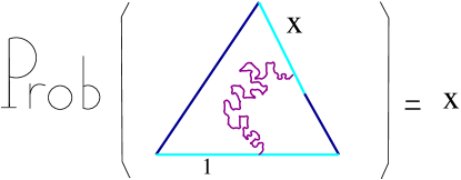
Figure 33: Crossing probability in a equilateral triangle.

It was later realized by Carleson (unpublished) that the formula becomes simpler if we look at it in a triangle instead in a rectangle. So let us consider site percolation in a triangular lattice with sites colored in black/white with probability 1/2 to ensure criticality. SLE and CFT deal with universal properties valid in the continuum limit in which the mesh of the lattice goes to zero. Formulas simplify if we look at percolation in an equilateral triangle with sides of length $1$ and with corners at positions $0$, $1$ and $e^{i\pi/3}$. Assume boundary conditions such that all sites on the bottom side $[0,1]$ of the triangle are black. Cardy’s formula is for the probability for the existence of clusters of black sites connecting the bottom side to a segment attached to the opposite corner $e^{i\pi/3}$ and of length $x<1$, see Fig.33. In this setting it becomes particularly simple as it is linear in $x$:

$${\bf P}[\ {\rm crossing~{}in~{}a~{}triangle}\ ]=x$$

This was proved by Smirnov [125] by actually considering a generalization of this probability involving a point in the bulk and not only on the boundary. Namely, with identical boundary conditions and given a point $z$ inside the triangle, he looked for the probability that there exists a path, included in a cluster of black sites, connecting the sides $[0,1]$ and $[1,e^{i\pi/3}]$ and leaving the point $z$ on its right. Smirnov’s proof is based on the observation that this probability is harmonic as a function of $z$. Namely:

$${\bf P}[\ {\rm cluster~{}on~{}the~{}left~{}of}~{}z\ ]=-\frac{2}{\sqrt{3}}\,\Im{\rm m}(z\,e^{-i\pi/3})$$

With $z$ approaching the boundary it reduces to Cardy’s formula.

Below, we present the derivation of Cardy’s formula using chordal SLE and that of Smirnov formula using dipolar SLE. However, we start with computations of hitting probabilities in order to exemplify the techniques. All these results, which require computing specific probabilities, can be found either using probabilistic or conformal field theory arguments. As usual with Markov processes, most of these probabilities may be computed by identifying the appropriate martingales. Since the SLE/CFT correspondence of Section 5.3 shows that SLE martingales are provided by ratios of CFT correlation functions, all these SLE probabilities can be expressed in terms ratio of CFT correlation functions. We shall alternatively use chordal, radial or dipolar SLEs to illustrate these facts.

7.1 Boundary hitting probabilities

Boundary hitting probabilities are the probabilities that the SLE curve visits a set of intervals on the real axis in a given order. We are going to show on a simple example how these probabilities are related to particular CFT correlation functions of boundary primary fields. These relations reveal connections between topological properties of SLE paths and fusion algebras and operator production expansions in conformal field theory.

We consider chordal SLE and we assume $4<\kappa<8$ so that the SLE trace touches the real axis infinitely many times with probability one. Consider the probability, first computed in [115], that the SLE curve touches an interval $[x,X]$ on the positive real axis. We shall compute its complement ${\bf P}[\gamma_{[0;\infty[}\cap[x,X]=\emptyset]$ that the curve does not touch the interval which is also equal to the probability that the two points $x$ and $X$ are swallowed at the same instant. The result is the following expression with $s=x/X$:

$${\bf P}[\gamma_{[0;\infty[}\cap[x,X]=\emptyset]=\frac{s^{\frac{\kappa-4}{\kappa}}\Gamma\left(\frac{4}{\kappa}\right)}{\Gamma\left(\frac{\kappa-4}{\kappa}\right)\Gamma\left(\frac{8-\kappa}{\kappa}\right)}\int_{0}^{1}d\sigma\sigma^{-\frac{4}{\kappa}}(1-s\sigma)^{2\frac{4-\kappa}{\kappa}}.$$ (55)

Its behavior as $X\to x$ gives the probability density for the SLE trace to touch the real axis in the neighborhood of the point $x$:

$${\bf P}[\gamma_{[0;\infty[}\cap[x,x+dx]\not=\emptyset]\propto\ (dx/|x|)^{{(8-\kappa)}/{\kappa}}$$

It agrees with the dimension $h_{1;3}=(8-\kappa)/\kappa$ of the operator coding for two SLE paths emerging from the real axis.

To simplify notation, let $p(x,X)\equiv{\bf P}[\gamma_{[0;\infty[}\cap[x,X]=\emptyset]$. By dimensional analysis it only depends on the ratio $x/X$ so that $p(x,X)=p(x/X,1)$. This probability is $0$ if $x\to 0$, or $X\to\infty$, and it is $1$ in the limit of coinciding points $X\to x$.

Let us start with the probabilistic argument. It is based on constructing an appropriate martingale using the Markov property of chordal SLE. Thus consider the probability that the SLE trace touches the interval $[x,X]$ conditioned on the knowledge of the SLE trace $\gamma_{[0;t[}$ up to time $t$ for $t<\tau_{x}$. As a conditional probability – and thus conditional expectation value – this is a martingale. Indeed, if we average it over $\gamma_{[0,t[}$ we reproduce the probability that the SLE trace touches the interval $[x,X]$. By Markov property we may start again the SLE process at time $t$ by erasing the SLE trace using the Loewner conformal map $h_{t}=g_{t}-\xi_{t}$. By conformal invariance the image of the rest of the SLE trace is then distributed as the original SLE trace but the point $x$ and $X$ have been moved to position $h_{t}(x)$ and $h_{t}(X)$. Hence this conditional probability is the probability that the SLE trace touches the interval $[h_{t}(x),h_{t}(X)]$:

$${\bf P}[\gamma_{[0;\infty[}\cap[x,X]=\emptyset\Big{|}\gamma_{[0;t[}]={\bf P}[\gamma_{[0;\infty[}\cap[h_{t}(x),h_{t}(X)]=\emptyset]$$

Because this conditional probability is a martingale, the drift term in its Itô derivative vanishes. It thus satisfies the second order differential equation:

$$\left(\frac{2}{x}\partial_{x}+\frac{2}{X}\partial_{X}+\frac{\kappa}{2}(\partial_{x}+\partial_{X})^{2}\right)p(x,X)=0.$$ (56)

Since it only depends on $s=x/X$ this translates into:

$$\left(\frac{d^{2}}{ds^{2}}+\left(\frac{4}{\kappa s}+\frac{2(4-\kappa)}{\kappa(1-s)}\right)\frac{d}{ds}\right)p(s,1)=0.$$

The integration is then straightforward with the normalization $p(s=0,1)=0$ and $p(s=1,1)=1$. It gives the formula (55) quoted above.

To illustrate the SLE/CFT correspondence we now re-derive this expression using CFT techniques. This is again based on exhibiting the appropriate martingale but now the latter is expressed in terms of CFT data [7]. To prepare for this computation, we study the CFT correlation function

$$\langle\psi_{1;2}|\varphi_{0}(X)\varphi_{0}(x)|\psi_{1;2}\rangle_{\mathbb{H}}.$$

For $4<\kappa<8$ we may choose it such that it vanishes as $x\to 0$ and takes value $1$ at $X\to x$. Indeed, if $x$ comes close to $0$, we can expand this function by computing the operator product expansion of $\varphi_{0}(x)|\psi_{1;2}\rangle$. This is constrained by the fusion rules which arise from the null vector $(4L_{-2}-{\kappa}L_{-1}^{2})|\psi_{1;2}\rangle=0$. It can involve at most two conformal families of dimension $h_{1;2}=\frac{6-\kappa}{2\kappa}$ or $h_{1;0}=\frac{\kappa-2}{\kappa}$. We demand that only the conformal family of dimension $h_{1;0}$ appears in the operator product expansion. Then, $\varphi_{0}(x)|\psi_{1;2}\rangle\sim x^{\frac{\kappa-4}{\kappa}}|\psi_{1;0}\rangle,$ with $|\psi_{1;0}\rangle$ the state created by $\psi_{1;0}(0)$. This goes to $0$ for $\kappa>4$. If the points $x$ and $X$ come close together, the operator product expansion $\varphi_{0}(X)\varphi_{0}(x)$ is more involved. General rules of conformal field theory ensure that the identity operator contributes, but apart from that, there is no a priori restrictions on the conformal families $\varphi_{\delta}$ that may appear. However, only those for which $\langle\psi_{1;2}|\varphi_{\delta}|\psi_{1;2}\rangle\neq 0$ remain, and this restricts to two conformal families, the identity and $\psi_{1;3}$. Namely, when $x$ and $X$ come close together,

$$\langle\psi_{1;2}|\varphi_{0}(X)\varphi_{0}(x)|\psi_{1;2}\rangle_{\mathbb{H}}\simeq 1+\cdots+\hat{C}\,(X-x)^{h_{1;3}}\,\langle\psi_{1;2}|\psi_{1;3}(x)|\psi_{1;2}\rangle_{\mathbb{H}}+\cdots$$

with $h_{1;3}=\frac{8-\kappa}{\kappa}$ and $\hat{C}$ some fusion coefficient. The dominant contribution to $\langle\psi_{1;2}|\varphi_{0}(X)\varphi_{0}(x)|\psi_{1;2}\rangle_{\mathbb{H}}$ is either $1$ or $(X-x)^{h_{1;3}}$, depending on whether $\kappa<8$ or $\kappa>8$. Hence, if $4<\kappa<8$, the correlation function vanishes as $x\to 0$ and takes value $1$ at $X\to x$.

Now, for nonzero $t$, we consider the CFT correlation function which is a martingale thanks to the statistical martinagle trick:

$$\langle\psi_{1;2}|\varphi_{0}(h_{t}(X))\varphi_{0}(h_{t}(x))|\psi_{1;2}\rangle_{\mathbb{H}}$$

If the position $a_{x}$ of the SLE trace at $t=\tau_{x}$ satisfies $x<a_{x}<X$, then $h_{\tau_{x}}(X)$ remains away from the origin but $\lim_{t\nearrow\tau_{x}}h_{t}(x)=0$ and the correlation function vanishes. On the other hand, if $X\leq a_{x}$, it is a general property of hulls that $\lim_{t\nearrow\tau_{x}}h_{t}(x)/h_{t}(X)=1$ and the correlation function is unity. Thus

$$\lim_{t\nearrow\tau_{x}}\langle\psi_{1;2}|\varphi_{0}(h_{t}(X))\varphi_{0}(h_{t}(x))|\psi_{1;2}\rangle_{\mathbb{H}}=\mathbf{1}_{\{\tau_{x}=\tau_{X}\}}.$$

with $\mathbf{1}_{\{\tau_{x}=\tau_{X}\}}$ the characteristic function of the events with $\tau_{x}=\tau_{X}$. From the martingale property extended to the stopping time $\tau_{x}$, we infer that the expectation values of this martingale is equal to its values at initial time. Since ${\bf E}[\mathbf{1}_{\{\tau_{x}=\tau_{X}\}}]$ is the probability that the curve does not touch the interval $[x,X]$ we get:

$${\bf P}[\gamma_{[0;\infty[}\cap[x,X]=\emptyset]=\langle\psi_{1;2}|\varphi_{0}(X)\varphi_{0}(x)|\psi_{1;2}\rangle_{\mathbb{H}}.$$ (57)

Furthermore, the fact that $\langle\psi_{1;2}|\varphi_{0}(X)\varphi_{0}(x)(-4L_{-2}+{\kappa}L_{-1}^{2})|\psi_{1;2}\rangle=0$ translates into a differential equation for the correlation function which coincides with eq.(56). See Appendix B. The differential operator annihilates the constants, a remnant of the fact that the identity operator has weight 0. With the chosen normalization for $\varphi_{0}(x)$, the relevant solution vanishes at the origin. The integration is then straightforward and it gives the formula (55).

This example is instructive, because it clearly shows how the CFT correlation functions are selected according to the topological behavior specified by the probabilities one computes. It shows in a fairly simple case that the thresholds $\kappa=4,8$ for topological properties of SLE appear in the CFT framework as thresholds at which divergences emerge in operator product expansions. Probability for visiting, in a given order, collections of intervals of the real axis are similarly related to CFT correlation functions with insertion a boundary operator of dimension zero at each end points of these intervals. Some of them have been explicitly computed in ref.[11]. However the general rules relating these probabilities to the specific conformal correlation functions, and thus to the specific intermediate families, have not been given yet.

7.2 Cardy’s crossing formulas

Cardy’s formula for critical percolation applies to SLE₆. It may be extended [90, 91, 92] to a formula valid for arbitrary $\kappa>4$. The problem is then formulated as follows. Consider chordal SLE. Let $-\infty<a<0<b<\infty$ and define the stopping times $\tau_{a}$ and $\tau_{b}$ as the first times at which the SLE trace touches the interval $(-\infty,a]$ and $[b,+\infty)$ respectively. By definition, the crossing probability is the probability that the trace hits first the interval $(-\infty,a]$ before it hits the interval $[b,+\infty)$, that is ${\bf P}[\tau_{a}<\tau_{b}].$ See Fig.34.

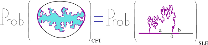
Figure 34: Crossing probability is identical to SLE swallowing probabilities.

The probabilistic argument is the same as in previous Section. Let $p_{c}(a,b)\equiv{\bf P}[\tau_{a}<\tau_{b}]$ be the crossing probability. By the Markov and identical increment properties of SLE, the process $t\to p_{c}(h_{t}(a),h_{t}(b))$ is a martingale. Hence the drift term of its Itô derivative vanishes. This yields the second order differential equation:

$$\left(\frac{2}{a}\partial_{a}+\frac{2}{b}\partial_{b}+\frac{\kappa}{2}(\partial_{a}+\partial_{b})^{2}\right)p(a,b)=0.$$

By scaling argument, $p_{c}(a,b)$ only depends on the ratio $r=-a/b>0$ with boundary condition $p_{c}(a=0,b)=1$, since then $a$ is clearly swallowed first, and $p_{c}(a,b=0)=0$, since then $b$ is swallowed first. Direct integration gives:

$$p_{c}(a,b)=\frac{\Gamma(2(\kappa-4)/\kappa)}{\Gamma((\kappa-4)/\kappa)^{2}}\ \int^{\infty}_{r}d\sigma\,\sigma^{-4/\kappa}(1+\sigma)^{2(4-\kappa)/\kappa},$$ (58)

with $r=-a/b$. This is proportional to the hypergeometric function:

$$p_{c}(a,b)=1-\frac{\kappa r^{1-4/\kappa}}{\kappa-4}\,_{2}F_{1}(\frac{4}{\kappa},1-\frac{4}{\kappa},2-\frac{4}{\kappa},\frac{r}{1+r})$$

For $\kappa=6$ it reduces to Cardy’s formula [27].

The CFT derivation is simpler than the one of previous Section. As it starts to become usual it consists in exhibiting the appropriate CFT martingale. So let us consider the following correlation function which, by the SLE/CFT correspondence, is a martingale:

$$F(h_{t}(a)/h_{t}(b))\equiv\langle\psi_{1;2}|\varphi_{0}(h_{t}(a))\varphi_{0}(h_{t}(b))|\psi_{1;2}\rangle_{\mathbb{H}}$$

with $\varphi_{0}$ a boundary conformal field of scaling dimension zero. By dimensional analysis it is only a function of the ratio $h_{t}(a)/h_{t}(b)$. There exist actually two linearly independent correlators, one of them being constant, but we shall not specify yet which non constant correlation function we pick. $F(a/b)$ can be computed explicitly, in terms of hypergeometric function, thanks to the null vector equation $(4L_{-2}-\kappa L_{-1}^{2})|\psi_{1;2}\rangle=0$.

The basic observation is that the ratio $h_{t}(a)/h_{t}(b)$ takes two simple non-random values depending whether $\tau_{a}<\tau_{b}$ or not, ie. depending whether the point $a$ have been surrounded by the SLE trace first or not. Let $\tau={\rm min}(\tau_{a},\tau_{b})$. If $\tau_{a}<\tau_{b}$, the point $a$ has been swallowed first so that $h_{\tau}(a)\simeq 0$ while $h_{\tau}(b)$ remains finite and thus $\lim_{t\nearrow\tau}\,h_{t}(a)/h_{t}(b)=0$. Similarly if $\tau_{b}<\tau_{a}$ then $\lim_{t\nearrow\tau}\,h_{t}(a)/h_{t}(b)=\infty$. Thus we have

$$\lim_{t\nearrow\tau}\,F(h_{t}(a)/h_{t}(b))={\bf 1}_{\{\tau_{a}<\tau_{b}\}}\,F(0)+{\bf 1}_{\{\tau_{a}>\tau_{b}\}}\,F(\infty).$$

Making the argument precise require checking that $F(0)$ and $F(\infty)$ are finite. As in previous Section, this follows from CFT fusion rules and it is true for $4<\kappa<8$. We can then compute $\lim_{t\nearrow\tau}\,{\bf E}[F(h_{t}(a)/h_{t}(b)]$ in terms of the swallowing probability ${\bf P}[\tau_{a}<\tau_{b}]$:

$$\lim_{t\nearrow\tau}\,{\bf E}[F(h_{t}(a)/h_{t}(b)]={\bf P}[\,\tau_{a}<\tau_{b}\,]\,F(0)+(1-{\bf P}[\,\tau_{a}<\tau_{b}]\,)\,F(\infty)$$

where we used that ${\bf P}[\,\tau_{a}>\tau_{b}\,]=1-{\bf P}[\,\tau_{a}<\tau_{b}\,]$. Applying the martingale property so that $\lim_{t\nearrow\tau}\,{\bf E}[\,F(h_{t}(a)/h_{t}(b))\,]=F(a/b)$, we get:

$${\bf P}[\,\tau_{a}<\tau_{b}\,]=\frac{F(a/b)-F(\infty)}{F(0)-F(\infty)}$$ (59)

For $\kappa=6$, this is Cardy’s formula [27]. In this form the formula is independent of the chosen normalization for $F$, but it can be further simplified by choosing boundary conditions on $F$ such that $F(0)=1$ and $F(\infty)=0$, which is possible for $4<\kappa<8$. It is very reminiscent of the probability for a one dimension Markov process driven by a stochastic differential equation to escape on a prescribed side of an interval containing its starting point.

7.3 Harmonic probabilities and Smirnov’s formula

Analogues of Smirnov’s formula give informations on bulk properties. For $\kappa>4$ they cannot be found using chordal or radial SLE because the hulls then invade the full domain. So we have to deal with dipolar SLE defined say in the strip $\mathbb{S}=\{z,\ 0<\Im{\rm m}z<\pi\}$ with marked point $x_{\pm}=\pm\infty$ and $x_{0}=0$.

We shall evaluate the probabilities $P_{l}(z,\bar{z})$ – resp. $P_{r}(z,\bar{z})$ – for a bulk point $z$ not to be swallowed by the SLE trace and to be on the left – resp. the right – of the trace. This is the probability for the point $z$ to be on the left – resp. the right – of the exterior frontier of the SLE hull viewed from the boundary point $x_{-}$ – resp. $x_{+}$. It is therefore the probability for the existence of a path joining $x_{-}$ – resp. $x_{+}$ – to the boundary interval $[x_{+},x_{-}]$ leaving the point $z$ on its right – resp. left – and included into one cluster of the underlying model of statistical mechanics. The result is [13]:

$$P_{l}(z,\bar{z})=1-\frac{\Im{\rm m}\,\hat{F}(z)}{\Im{\rm m}\,\hat{F}(\infty)},\quad\hat{F}(z)\equiv\int_{-\infty}^{z}\frac{du}{(\sinh u/2)^{4/\kappa}}.$$ (60)

A noticeable property is that it is a harmonic function. For $\kappa=6$ it reproduces Smirnov’s formula [125]. At the end of this Section we give another formula for the probability for the point $z$ to be in the SLE hull.

The function $\hat{F}(z)$ has a nice geometrical interpretation: it uniformizes the strip onto a triangle with corners $\hat{F}(-\infty)=0$, $\hat{F}(+\infty)=e^{-i2\pi/\kappa}I$ and $\hat{F}(0)=e^{-i4\pi/\kappa}J$ with $I=\int_{-\infty}^{+\infty}dy(\cosh y/2)^{-4/\kappa}$ and $J=\int_{0}^{\infty}dy(\sinh y/2)^{-4/\kappa}$. We have $I=2J\cos(2\pi/\kappa)$. The geometry becomes even simpler in the case $\kappa=6$ because the triangle is then equilateral. This explains why Smirnov’s formula is simply linear in an equilateral triangle. More on the relation between SLE$(\kappa,\rho)$ and triangle may be found in ref.[44].

As usual, a way to compute these probabilities is to notice that the process $t\to P(h_{t}(z),\overline{h_{t}(z)})$ is a local martingale. Indeed, since $h_{s}\circ h_{t}^{-1}$, $s>t$, is independent of $h_{t}$ and distributed as $h_{s-t}$, the function $P(h_{t}(z),\overline{h_{t}(z)})$ is the wanted probability conditioned on the process up to time $t$ and, as such, it is a martingale. As a consequence, the drift term in its Itô derivative vanishes which implies that $P(z,\bar{z})$ satisfies the following differential equation:

$$\kappa\partial_{z}\bar{\partial}_{\bar{z}}P+(\coth\frac{z}{2}+\frac{\kappa}{2}\partial_{z})\partial_{z}P+(\coth\frac{\bar{z}}{2}+\frac{\kappa}{2}\partial_{\bar{z}})\partial_{\bar{z}}P=0.$$

Quite remarkably this equation has enough harmonic solutions to compute $P_{l}$ and $P_{r}$. For the probability to be on the left of the hull, the boundary conditions are: $P_{l}(-\infty)=1$, $P_{l}(+\infty)=0$ and $P_{l}(0)=0$. Similar conditions hold for $P_{r}$. That these boundary conditions are enough to specify a unique solution is due to the fact that this equation is of second order in $\Re{\rm e}\;z$ but only first order in $\Im{\rm m}\;z$, so that boundary conditions at three points are enough to fix the function on the whole boundary. They follow by noticing that if point $z$ is swallowed at time $\tau_{z}$ then $\lim_{t\nearrow\tau_{z}}h_{t}(z)=0$, if it is not swallowed but is on the left of the trace then $\lim_{t\nearrow\infty}h_{t}(z)=-\infty$, and if it is not swallowed but is on the right of the trace then $\lim_{t\nearrow\infty}h_{t}(z)=+\infty$. These conditions are such that at the stopping $\widehat{\tau}_{z}={\rm min}(\tau_{z},\infty)$ the martingale $P(h_{t}(z),\overline{h_{t}(z)})$ projects on the appropriate events.

The solution of the martingale equation satisfying the appropriate boundary conditions is clearly given by the harmonic function (60). The function $\hat{F}(z)$ is well-defined and analytic on the strip $\mathbb{S}$ for all $\kappa$’s. For $\kappa>4$, $\hat{F}(z)$ is bounded and has a continuous extension to the closure of the strip. As a check one may verify that $P_{l}(z,\bar{z})$ behaves as expected on the boundary. On the positive real axis, $(\sinh z/2)$ is real and positive so that $P_{l}(x)=0$ for $x\in\mathbb{R}_{+}$, in accordance with the fact that no point on the real axis can be on the left of the trace. On the negative real axis, $(\sinh x/2)^{4/\kappa}=e^{i4\pi/\kappa}(\sinh|x|/2)^{4/\kappa}$ and

$$P_{l}(x)=1-\frac{1}{J}\int_{|x|}^{+\infty}\frac{dy}{(\sinh y/2)^{4/\kappa}},\quad x\in\mathbb{R}_{-},$$

It gives the probability of the hull not to spread further than $x$ on the negative real axis. On the upper boundary,

$$P_{l}(z=i\pi+x)=1-\frac{1}{I}\int_{-\infty}^{x}\frac{dy}{(\cosh y/2)^{4/\kappa}},\quad z\in i\pi+\mathbb{R},$$ (61)

since there $(\sinh z/2)^{4/\kappa}=e^{2i\pi/\kappa}(\cosh x/2)^{4/\kappa}$. This yields the density probability for the trace to stops on an interval $[x,x+dx]$ on the upper boundary.

For $\kappa=4$ the SLE trace is a simple curve so that no point away from the curve is swallowed in a finite time. This case is marginal in the sense that the integral defining $\hat{F}(z)$ is only logarithmically divergent. By extension, we have:

$$P_{l}(z,\bar{z})=\frac{1}{\pi}\Im{\rm m}\,\left[\log(\tanh\frac{z}{4})\right].$$ (62)

This satisfies the martingale equation for $\kappa=4$ and the appropriate boundary conditions: $P_{l}(x\in\mathbb{R}_{+})=0$ and $P_{l}(x\in\mathbb{R}_{-})=1$. Contrary to the cases $\kappa>4$, it is discontinuous at the origin. On the upper boundary the distribution of the trace is given by:

$$P_{l}(i\pi+x)=1-\frac{2}{\pi}\arctan(e^{x/2}),\quad x\in\mathbb{R}.$$

The probability (62) possesses a nice free field CFT interpretation. For $\kappa=4$, the Virasoro central charge is $c=1$ and $h_{1;2}=1/4$ and $h_{0;1/2}=1/16$. Central charge $c=1$ corresponds to bosonic free field. Let us denote by $X$ this field. $h_{1;2}=1/4$ is the conformal weight of the boundary vertex operator $V_{1;2}=\cos X/\sqrt{2}$ which may be thought of as the boundary condition changing operator intertwining two boundary intervals on which two different Dirichlet boundary conditions are imposed. $h_{0;1/2}=1/16$ is the dimension of the twist field $\sigma$ which is the boundary condition changing operator intertwining between Dirichlet and Neumann boundary conditions. Thus the probability $P_{l}(z,\bar{z})$ is proportional to the free field expectation value

$$\langle X(z,\bar{z})\rangle_{\mathbb{S},\,D;D;N}=\langle\sigma(x_{+})\sigma(x_{-})X(z,\bar{z})V_{1;2}(x_{0})\rangle_{\mathbb{S}},$$

where ’D;D;N’ refers to Dirichlet boundary conditions on the lower boundary $[x_{-},x_{0}]$ and $[x_{0},x_{+}]$, but with a discontinuity at $x_{0}$ and Neumann boundary condition on the upper boundary $[x_{-},x_{+}]$. The fact $P_{l}(z,\bar{z})$ satisfies the Dirichlet boundary conditions on the lower boundary is clear by construction but one may verify that it actually satisfies the Neumann boundary condition on the upper boundary. The fact that it is a harmonic function is then a consequence of the free field equation of $X$.

For $\kappa>4$, these probabilities are proportional to the CFT correlation functions

$$\langle\psi_{0;1/2}(x_{-})\psi_{0;1/2}(x_{+})\Phi_{0}(z,\bar{z})\psi_{1;2}(x_{0})\rangle_{\mathbb{S}}$$

involving a weight zero bulk primary field $\Phi_{0}$. This operator $\Phi_{0}$ has a simple interpretation in the Coulomb gas formulation [42, 41] of CFT: it a linear combination of the primitive of the screening current $Q_{-}$ and the identity operator, ie:

$$\Phi_{0}(z,\bar{z})={\rm const^{\prime}.}\,{\bf 1}+\Re{\rm e}\,[\,{\rm const.}\,\int^{z}dw\,Q_{-}(w)\,].$$

Indeed this operator has conformal weight zero, satisfies the appropriate fusion rules and fulfills the charge conservation requirement which demands that the sum of the coulomb charges of the operators involve in the correlation function minus the background charge belongs to the lattice generated by the screening charges.

Similarly, we may compute the probability $P_{in}(z,\bar{z})$ for the point $z$ to be in the SLE hull for $\kappa>4$. We do not distinguish the events in which the point has been swallowed from the right or from the left. It is solution of the same second order differential equation as $P_{l}$ but with different boundary conditions: $P_{in}(\pm\infty)=0$ and $P_{in}(0)=1$. The result is:

$$P_{in}(z,\bar{z})=\frac{\Im{\rm m}[e^{i2\pi/\kappa}\,\hat{F}(z)\,]}{\Im{\rm m}[e^{i2\pi/\kappa}\,\hat{F}(0)\,]}$$ (63)

with same function $\hat{F}(z)$ as above. We have: $\Im{\rm m}[e^{i\frac{2\pi}{\kappa}}\hat{F}(0)]=-\sin(\frac{2\pi}{\kappa})\,J$. Again, $P_{in}$ has the expected behavior on the boundary. Since $e^{i2\pi/\kappa}\,F(z)$ is real on the upper boundary, we have $P_{in}(z,\bar{z})=0$ for $z\in i\pi+\mathbb{R},$ in agreement with the fact that no point on the upper boundary can be swallowed. $P_{in}$ is even on the real axis and

$$P_{in}(x)=\frac{1}{J}\int_{|x|}^{+\infty}\frac{dy}{(\sinh y/2)^{4/\kappa}},\quad x\in\mathbb{R}.$$

This is of course complementary to $P_{l}(x)$ for $x$ negative.

For $\kappa<4$ the SLE trace is a simple curve so that the probability to be inside the hull has no meaning but one may still try to evaluate the probability to be on the left, or on the right, of the trace. It turns out that these probabilities are not any more harmonic functions. However, the probability to hit the upper boundary is still given by formula (61), as proved in [13]. It is has been numerically check in the case of the Ising model in [13].

7.4 Fractal dimensions

The fractal dimension of a set may be defined via box counting. Let $N_{\varepsilon}$ be the number of boxes of typical linear size $\varepsilon$ needed to cover the set. This number increases as $\varepsilon\to 0$ and – if it exists – we may define the fractal dimension $d_{\kappa}$ by $d_{\kappa}=-\lim_{\varepsilon\to 0}\log N_{\varepsilon}/\log\varepsilon$, ie. $N_{\varepsilon}$ follows the power law $N_{\varepsilon}\approx\varepsilon^{-d_{\kappa}}$. In our case, the set is a curve. Imagine that this curve is inscribed in a domain of typical size $L$ which may be covered by $(L/\varepsilon)^{D}$ boxes of size $\varepsilon$ – in two dimensions $D=2$. To cover the curve we need $N_{\varepsilon}\approx(L/\varepsilon)^{d_{\kappa}}$ so that the probability to find the curve in one of the infinitesimal box scales as $\varepsilon^{D-d_{\kappa}}$. This is the strategy we follow to compute the fractal dimension of the SLE curves. Namely we evaluate the probability that the SLE path approaches a bulk point $z_{0}$ at a distance less than $\varepsilon$:

$${\bf P}[\gamma_{[0,+\infty)}\cap\mathbb{B}_{\varepsilon}(z_{0})\not=\emptyset]\approx\varepsilon^{2-d_{\kappa}},\quad\varepsilon\to 0$$

with $\mathbb{B}_{\varepsilon}(z_{0})$ the ball of radius $\varepsilon$ centered in $z_{0}$. As already mentioned, this yields:

$$d_{\kappa}=1+\kappa/8,\ {\rm for}\ \kappa<8,\quad\quad d_{\kappa}=2,\ {\rm for}\ \kappa>8$$

This formula was predicted by B. Duplantier [59, 60] and rigorously proven by V. Beffara [19, 20]. See also [52] in the case of percolation ($\kappa=6$ and $8/3$). The complete determination of $d_{\kappa}$ requires also establishing a two point estimate, which is much harder to obtain but which may be found in the nice reference [20].

Computing this probability is done, as usual, by identifying the appropriate martingale using either probabilistic or CFT arguments. It leads to the identification of the conformal primary field $\Phi_{0;1}(z_{0},\bar{z}_{0})$ of bulk scaling dimension $2h_{0;1}=\frac{8-\kappa}{8}$ as the field conditioning on the presence of a SLE curve in the neighborhood of the point $z_{0}$.

We use chordal SLE in the upper half plane. So let $z_{0}\in\mathbb{H}$, $\Im{\rm m}z_{0}>0$, be a point in the upper half plane and $\delta_{t}(z_{0})$ its distance to the SLE curve $\gamma_{[0,t]}$ stopped at time $t$. We shall evaluate $\delta_{t}(z_{0})$ using the conformal radius of $\gamma_{[0,t]}$ seen from $z_{0}$. To compute it, let $k_{t}(z)$, defined by

$$k_{t}(z)=\frac{g_{t}(z)-g_{t}(z_{0})}{g_{t}(z)-\overline{g_{t}(z_{0})}},$$

be a uniformizing map of $\mathbb{H}\setminus\mathbb{K}_{t}$ onto the unit disk with $k_{t}(z_{0})=0$, $k_{t}(\infty)=1$. The conformal radius of $\gamma_{[0,t]}$ viewed from $z_{0}$ is defined as $\rho_{t}(z_{0})\equiv|k_{t}^{\prime}(z_{0})|^{-1}$. An explicit computation gives $\rho_{t}(z_{0})=|2\Im{\rm m}h_{t}(z_{0})/h^{\prime}_{t}(z_{0})|$ with $h_{t}=g_{t}-\xi_{t}$. Köbe $1/4$-theorem states that $(1/4)\rho_{t}(z_{0})\leq\delta_{t}(z_{0})\leq\rho_{t}(z_{0})$ so that $\delta_{t}(z_{0})$ and $\rho_{t}(z_{0})$ scale the same way. One may check that $\rho_{t}(z_{0})$ is always decreasing as time goes by. So instead of estimating the distance between the SLE path and $z_{0}$, we shall estimate its conformal radius, $\rho(z_{0},\gamma)=\lim_{t\to\tau_{z_{0}}}\rho_{t}(z_{0})$, and the probability ${\bf P}[\rho(z_{0},\gamma)\leq\varepsilon]$.

The image $U_{t}\equiv k_{t}(\gamma(t))$ of the tip of the curve by $k_{t}$ is on the unit circle. Setting $U_{t}\equiv e^{i\alpha_{t}}$ defines a process $\alpha_{t}$ on the unit circle with $\alpha_{t}\to 0$ or $2\pi$ as $t\to\tau_{z_{0}}$ depending whether $z_{0}$ has been swallowed clockwise, or counterclockwise, by the SLE trace. Actually, up to a random time reparametrization, $ds=(\frac{2\Im{\rm m}h_{t}(z_{0})}{|h_{t}(z_{0})|^{2}})^{2}dt$, this process is driven by $d\alpha_{s}=\frac{\kappa-4}{4}\cot(\alpha_{s}/2)+d\xi_{s}$. Estimating ${\bf P}[\rho(z_{0},\gamma)\leq\varepsilon]$ can be formulated [20] as a survival probability problem for the process $\alpha_{s}$ but, in order to understand its CFT origin, we shall compute it using a CFT martingale. For $\kappa<8$, let us consider the expectation value

$$\hat{M}_{t}(z_{0})\equiv|h_{t}^{\prime}(z)|^{2h_{0;1}}\,\langle\psi_{1;2}|\Phi_{0;1}(h_{t}(z_{0}),\bar{h_{t}(z_{0})})|\psi_{1;2}\rangle_{\mathbb{H}}$$

with $\Phi_{0;1}$ the bulk conformal field of weight $2h_{0;1}=(8-\kappa)/8$. By construction this is well defined up to time $t<\tau_{z_{0}}$. The correlation function $\langle\psi_{1;2}|\Phi_{0;1}(z_{0},\bar{z}_{0})|\psi_{1;2}\rangle$ may be computed exactly using the level two null vector. It is equal to $|2\Im{\rm m}z_{0}|^{-2h_{0;1}}(\sin\alpha_{0}/2)^{8/\kappa-1}$ with $z_{0}/\bar{z}_{0}=e^{i\alpha_{0}}$ so that

$$\hat{M}_{t}(z_{0})=\Big{|}\frac{h^{\prime}_{t}(z_{0})}{2\Im{\rm m}h_{t}(z_{0})}\Big{|}^{2h_{0;1}}\,(\sin\alpha_{t}/2)^{\kappa/8-1}=\rho_{t}(z_{0})^{-2h_{0;1}}\,(\sin\alpha_{t}/2)^{8/\kappa-1}$$

Let $\tau_{z_{0}}^{\varepsilon}$ be either the time at which the conformal radius $\rho_{t}(z_{0})$ reaches the value $\varepsilon$, if $\rho(z_{0},\gamma)\leq\varepsilon$, or the swallowing time $\tau_{z_{0}}$ if the point $z_{0}$ is swallowed before the conformal radius reaches this value, i.e. if $\rho(z_{0},\gamma)>\varepsilon$. The time $\tau_{z_{0}}^{\varepsilon}$ is a stopping time. Since $h^{\prime}_{t}(z_{0})$ vanishes faster than $h_{t}(z_{0})$ as $t\to\tau_{z_{0}}$, the martingale $\hat{M}_{t}(z_{0})$ vanishes as $t\to\tau_{z_{0}}$ for $\kappa<8$. Therefore as time $t$ approaches $\tau_{z_{0}}^{\varepsilon}$, the martingales $\hat{M}_{t}(z_{0})$ projects on configuration with the curve at a distance from $z_{0}$ less than $\varepsilon$, ie.:

$$\hat{M}_{\tau_{z_{0}}^{\varepsilon}}(z_{0})=\varepsilon^{-2h_{0;1}}\,(\sin\alpha_{\tau_{z_{0}}^{\varepsilon}}/2)^{8/\kappa-1}\ {\bf 1}_{\{\rho(z_{0},\gamma)\leq\varepsilon\}}$$

Up to the angular dependence $(\sin\alpha_{\tau_{z_{0}}^{\varepsilon}}/2)^{8/\kappa-1}$, which does not play any role in the scaling analysis, $\hat{M}_{\tau_{z_{0}}^{\varepsilon}}(z_{0})$ is proportional to the characteristic function of the set of curve passing at distance $\varepsilon$ from $z_{0}$ so that its expectation behaves as the probability ${\bf P}[\rho(z_{0},\gamma)<\varepsilon]$. By construction $\hat{M}_{t}(z_{0})$ is a martingale so that ${\bf E}[\hat{M}_{\tau_{z_{0}}^{\varepsilon}}(z_{0})]=\hat{M}_{t=0}(z_{0})$ and

$${\bf P}[\rho(z_{0},\gamma)\leq\varepsilon]\approx\varepsilon^{2h_{0;1}}$$

as $\varepsilon\to 0$. This one point estimate yields to the fractal dimension $d_{\kappa}=2-2h_{0;1}$ or equivalently $d_{\kappa}=1+\kappa/8$.

More generally, one may look for the zig-zag density probabilities that the SLE paths visit balls $\mathbb{B}_{\varepsilon}(z_{p})$ centered in points $z_{p}$. This is clearly proportional to CFT correlation functions $\langle\psi_{1;2}|\Phi_{0;1}(z_{1},\bar{z}_{1})\cdots\Phi_{0;1}(z_{n},\bar{z}_{n})|\psi_{1;2}\rangle$. Different orders of visiting the points $z_{p}$ corresponds to different correlation functions alias conformal blocks. If no order among the visited balls is specified, these correlation functions have no monodromy and they thus correspond to the complete CFT correlation functions. Zig-zag probabilities with specified ordering in the visits would be exchanged as one moves the points $z_{p}$ around. In other words, there is probably a quite direct relation between CFT monodromies, quantum groups, and braiding properties of samples of SLE traces.

7.5 Miscellaneous

An important output of SLE was the mathematical proof [90, 91, 91] for the values of the Brownian intersection exponents. See the comprehensible reviews [133, 99]. Many of these exponents have been predicted using techniques from conformal field theory, see for instance [51, 53, 4]. These exponents describe how the probabilities for a set of Brownian paths not to intersect decreases with time. Let $B_{t}^{j}$, $j=1,\cdots,n$ be $n$ independent planar Brownian motions started from $n$ different points in the plane and run during a time $t$. The probability that they do not intersect decreases as $t^{-\zeta_{n}}$ with $\zeta_{n}=(4n^{2}-1)/24$. The same probability but for Brownian motions confined in the upper half plane decreases with time as $t^{-\tilde{\zeta}_{n}}$ with $\tilde{\zeta}_{n}=n(2n+1)/6$. More generally, one may look at the non intersecting probabilities of $k$ packs of Brownian motions, each of them made of $n_{j}$, $j=1,\cdots,k$, independent Brownian motions started from distinct points. These probabilities decrease with time with exponents $\zeta_{n_{1},\cdots,n_{k}}$ and $\tilde{\zeta}_{n_{1},\cdots,n_{k}}$ depending whether the Brownian paths are in the plane or in the upper half plane. Although many properties of these exponents [133, 99] were known – such that the cascade relations they satisfy [87] and more [88, 89, 126] – the exactness of CFT predictions [51, 53, 4] was proved only recently by Lawler, Schramm and Werner [90, 91, 92] using SLE. The proof of these results relies on a universality argument [89] which states that any conformally invariant process satisfying the restriction property has crossing and intersection exponents that are intimately related to the Brownian intersection exponents. As the boundary of SLE₆ is conformally invariant and satisfies the restriction property, the computation of its exponents yields the Brownian intersection exponents. The relation between SLE₆ and Brownian motion is even more precise in the sense that the hull generated by SLE₆ is the same as the hull generated by a Brownian motion with oblique reflection [135].

Cardy’s crossing formula [27] for percolation, its proof by Smirnov [125] and the numerical simulations of [85] did play an important in the birth of SLEs. Another crossing formula for percolation has been predicted by Watts using CFT argument [132]. This formula, which was also motivated by the numerical analysis of [85], gives the probability in critical percolation that there exists a percolating clusters crossing simultaneously from the right to left and from top to bottom of rectangle. Although Watts’s formula remained conjectural for a while it has now been proved in [47] using excursion decompositions of SLEs. Crossing formula for critical percolation in an annulus have also been predicted by Cardy using CFT [31]. Their SLE companions have been derived in [45]. Finally, another excursion formula for percolation has been proved using SLE in [119].

The one-arm exponent which governs the decrease of the probability that the critical percolating cluster has diameter of order $R$ – this probability behaves as $R^{-5/48}$ – has been SLE proved in [94]. A two-arm exponent, also called backbone exponent, which describes the decrease of the probability that there are two disjoint open crossings from a circle of radius $r$ to a circle of radius $R$ has been estimated in [92]. This prediction is yet out of reach of conformal field theory.

The proof that the scaling limit of loop erased random walks and uniform spanning trees are respectively SLE₂ and $SLE_{8}$ are given in refs.[118, 95]. Although there is no much doubt, there is yet no mathematical proof that self-avoiding walks converge to SLE_8/3 in the continuum limit, but see ref.[96]. More informations on spanning trees and related domino tilling may be found in ref.[81].

8 Other growth processes

This Section deals with more general 2D growth processes than SLEs. Although, they do not fulfill the local growth and conformal invariance properties of SLEs, they are nevertheless described by dynamical conformal maps. We first present systems whose conformal maps have a time continuous evolution and give examples. We then go on by presenting a discrete version thereof in terms of iterated conformal maps. This field of research is much less developed and understood, at least mathematically, than SLEs. There are many questions still unanswered today.

Examples of models – including DLA, dielectric breakdown, Hele-Shaw problems, etc. – have been introduced in Section 2.4. They have a large domain of applicability [22, 65, 68, 18, 130] and many examples have been given in Section 2.4. We shall elaborate more on them. They are all linked to Laplacian growth which is one of the simplest examples of such growth processes. We shall spend more times on Laplacian growth since it is a rich system which possesses an underlying integrable structure but which simultaneously produces singularities leading to dendritic growth.

In this part, the exterior of the unit disk, $\mathbb{U}=\{w\in\mathbb{C},\ |w|>1\}$, is used as the reference geometry. So the growth dynamics are going to be described by radial Loewner chains, simple variants of the chordal Loewner chains.

We end this Section by a brief discussion of discrete Loewner chains defined by iterations of conformal maps.

8.1 Radial Loewner chains

Let $\mathbb{K}_{t}$ be a family of growing closed planar sets such that their complement in the complex plane $\mathbb{O}_{t}\equiv\mathbb{C}\setminus\mathbb{K}_{t}$ also have the topology of a disk. See Fig.35. To fix part of translation invariance we assume that the origin belongs to $\mathbb{K}_{t}$ and the point at infinity to $\mathbb{O}_{t}$.

Loewner chains describe the evolution of family of conformal maps $f_{t}$ uniformizing $\mathbb{U}=\{w\in\mathbb{C};\ |w|>1\}$ onto $\mathbb{O}_{t}$. It thus describes the evolution of the physical domains $\mathbb{O}_{t}$. We normalize the maps $f_{t}:\mathbb{U}\to\mathbb{O}_{t}$ by demanding that they fix the point at infinity, $f_{t}(\infty)=\infty$ and that $f_{t}^{\prime}(\infty)>0$. With $t$ parameterizing time, Loewner equation for the evolution of $f_{t}$ reads:

$$\frac{\partial}{\partial t}f_{t}(w)=wf_{t}^{\prime}(w)\,\oint\frac{\rho_{t}(u)du}{2i\pi u}\,\Big{(}{\frac{w+u}{w-u}}\Big{)}$$ (64)

The integration is over the unit circle $\{u\in\mathbb{C},|u|=1\}$. The Loewner density $\rho_{t}(u)$ codes for the time evolution. It may depends on the map $f_{t}$ in which case the growth process in non-linear. For the inverse maps $g_{t}\equiv f_{t}^{-1}:\mathbb{O}_{t}\to\mathbb{U}$, Loewner equation reads:

$$\frac{\partial}{\partial t}g_{t}(z)=-g_{t}(z)\oint\frac{\rho_{t}(u)du}{2i\pi u}\Big{(}{\frac{g_{t}(z)+u}{g_{t}(z)-u}}\Big{)}$$ (65)

Compare with the equation governing radial SLE.

The behavior of $f_{t}$ at infinity fixes a scale since at infinity, $f_{t}(w)\simeq R_{t}w+O(1)$ where $R_{t}>0$, with the dimension of a [length], is called the conformal radius of $\mathbb{K}_{t}$ viewed from infinity. $R_{t}$ may be used to analyze scaling behaviors, since Kobe 1/4-theorem (see e.g. [39, 2]) ensures that $R_{t}$ scales as the size of the domain. In particular, the (fractal) dimension $D$ of the domains $\mathbb{K}_{t}$ may be estimated by comparing their area $\mathcal{A}_{t}$ with their linear size measured by $R_{t}$: $\mathcal{A}_{t}\asymp R_{t}^{D}$ for large $t$ – the proportionality factor contains a cutoff dependence which restores naive dimensional analysis.

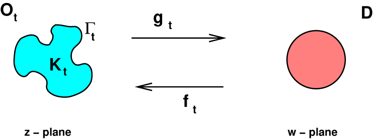
Figure 35: Uniformizing maps intertwining the ‘physical’ $z$-plane and the ‘mathematical’ $w$-plane.

The boundary curve $\Gamma_{t}\equiv\partial\mathbb{O}_{t}$ is the image of the unit circle by $f_{t}$. We may parameterize the boundary points by $\gamma_{t;\alpha}=f_{t}(u)$ with $u=e^{i\alpha}$. The Loewner equation codes for the evolution of the shape of $\mathbb{O}_{t}$ and thus for the normal velocity of the boundary points. Only the normal velocity is relevant as the tangent velocity is parameterization dependent. The tangent to the curve is $\tau=iuf_{t}^{\prime}(u)/|f_{t}^{\prime}(u)|$ and the outward normal is $n=-i\tau$ so that the normal velocity at $\gamma_{t}$ is $v_{n}=\Re{\rm e}[\bar{n}\,\partial_{t}f_{t}(u)]$, or

$$v_{n}=|f_{t}^{\prime}(u)|\,\Re{\rm e}[\partial_{t}f_{t}(u)/uf_{t}^{\prime}(u)].$$

The r.h.s. is determined by the Loewner equation (64) because this equation may be viewed as providing the solution of a boundary value problem. Indeed, recall that for $\hat{h}(u)$ a real function on the unit circle, $h(w)=\oint\frac{du}{2i\pi u}\Big{(}\frac{w+u}{w-u}\Big{)}\hat{h}(u)$ is the unique function analytic outside the unit disk whose real part on the unit circle is $\hat{h}$. Thus, since $\partial_{t}f_{t}(w)/wf_{t}^{\prime}(w)$ is analytic in $\mathbb{U}$, the Loewner equation (64) is equivalent to:

$$v_{n}=|f_{t}^{\prime}(u)|\,\rho_{t}(u)$$

or more explicitly:

$$(\partial_{\alpha}\gamma_{t;\alpha})\,(\partial_{t}\overline{\gamma_{t;\alpha}})-(\partial_{\alpha}\overline{\gamma_{t;\alpha}})\,(\partial_{t}\gamma_{t;\alpha})=2i\,|f_{t}^{\prime}(u)|^{2}\,\rho_{t}(u)$$ (66)

Hence, the evolution of the domain may be encoded either in the evolution law for its uniformizing conformal map as in eq.(64) or in the boundary normal velocity as in eq.(66). The two equations are equivalent.

8.2 Laplacian growth as a Loewner chain

8.2.1 Basics

Laplacian growth (LG) is a process in which the growth of the domain is governed by the solution of Laplace equation, i.e. by an harmonic function, in the exterior of the domain with appropriate boundary conditions. It originates from the hydrodynamic Hele-Shaw problem to be described below, see eg. [22].

To be precise, let $P$ be the real solution of Laplace equation, $\nabla^{2}P=0$, in $\mathbb{O}_{t}$ with the boundary behavior $P=-\log|z|+\cdots$ at infinity and $P=0$ on the boundary curve $\Gamma_{t}=\partial\mathbb{O}_{t}$. The time evolution of the domain is then defined by demanding that the normal velocity of points on the boundary curve be equal to minus the gradient of $P$: $v_{n}=-(\nabla P)_{n}$.

This problem may be written as a Loewner chain since, as is well known, Laplace equation is solved via complex analysis by writing $P$ as the real part of an analytic function. One first solves Laplace equation in the complement of the unit disk with the appropriate boundary conditions and then transports it back to the physical domain $\mathbb{O}_{t}$ using the map $f_{t}$. This gives:

$$P=-\Re{\rm e}\ \Phi_{t}\quad{\rm with}\quad\Phi_{t}(z)=\log g_{t}(z)$$

The evolution equation for the map $f_{t}$ is derived using that the boundary normal velocity is $v_{n}=-(\nabla P)_{n}$. The above expression for $P$ gives:

$$v_{n}=-(\nabla P)_{n}=|f_{t}^{\prime}(u)|^{-1}$$

at point $\gamma_{t}=f_{t}(u)$ on the boundary curve. As explained in the previous Section, this is enough to determine $\partial_{t}f_{t}(w)$ for any $|w|>1$ since this data specifies the real part on the unit circle of the analytic function $\partial_{t}f_{t}(w)/wf_{t}^{\prime}(w)$ on the complement of the unit disk. The result is:

$$\partial_{t}f_{t}(w)=wf_{t}^{\prime}(w)\,\oint_{|u|=1}\frac{du}{2i\pi u\,|f_{t}^{\prime}(u)|^{2}}\Big{(}{\frac{w+u}{w-u}}\Big{)}$$ (67)

It is a Loewner chain with $\rho_{t}(u)=|f_{t}^{\prime}(u)|^{-2}$.

As we shall see below, Laplacian growth is an integrable system, which may be solved exactly, but it is ill-posed as the domain develops singularities (cusps $y^{2}\simeq x^{3}$) in finite time. It thus needs to be regularized. There exist different ways of regularizing it.

A larger class of problems generalizing Laplacian growth have been introduced. Their Loewner measures are as in Laplacian growth but with a different exponent:

$$\rho_{t}(u)=|f_{t}^{\prime}(u)|^{-\alpha}\quad,\quad 0\leq\alpha\leq 2.$$

Using an electrostatic interpretation of the harmonic potential, one usually refers to the case $\alpha=1$ as a model of dielectric breakdown because the measure is then proportional to the local electric field $E_{n}=|f_{t}^{\prime}(u)|^{-1}$. This is a phenomenological description. Just as the naive Laplacian growth these models are certainly ill-posed. They also require ultraviolet regularization.

8.2.2 Singularities

The occurrence of singularities in Laplacian growth may be grasped by looking for the evolution of domains with a $Z_{n}$ symmetry uniformized by the maps

$$f_{t}(w)=R_{t}w(1+\frac{\beta_{t}}{n-1}w^{-n})$$

for some $n>2$ and with $|\beta_{t}|\leq 1$. This form of conformal maps is preserved by the dynamics. The conformal radius $R_{t}$ and the coefficients $\beta_{t}$ evolve with time according to $\partial_{t}R^{2}_{t}=2/(1-\beta_{t}^{2})$ and $\beta_{t}=(R_{t}/R_{c})^{n-2}$ with $R_{c}$ some integration constant. The singularity appears when $\beta_{t}$ touches the unit circle which arises at a finite time $t_{c}$. At that time the conformal radius is $R_{c}$.

At $t_{c}$ the boundary curve $\Gamma_{t_{c}}$ has cusp singularities of the generic local form

$$\ell_{c}\,(\delta y)^{2}\simeq(\delta x)^{3}$$

with $\ell_{c}$ a characteristic local length scale. In the present simple case $\ell_{c}\simeq R_{c}$. At time $t\nearrow t_{c}$, the dynamics is regular in the dimensionless parameter $\ell_{c}^{-1}\sqrt{t_{c}-t}$. The maximum curvature of the boundary curve scales as $\kappa_{\rm max}\simeq{\ell_{c}}/{(t_{c}-t)}$ near $t_{c}$ and it is localized at a distance $\sqrt{t_{c}-t}$ away from the would be cusp tip. See Fig.36.

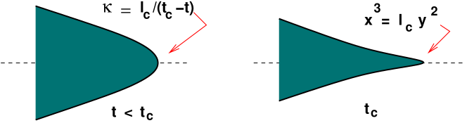
Figure 36: Cups formation in Laplacian growth.

This behavior is quite generic. Conformal maps $f_{t}(w)$ such that their derivatives are polynomials in $w^{-1}$ are stable by the Laplacian growth dynamics. By construction, their zeroes are localized inside the unit disk. A singularity in the boundary curve occurs if one of these zeroes converges to the unit circle. The singularity is then a cusp $\ell_{c}\,y^{2}\simeq x^{3}$ as can be seen by expanding locally the conformal map around its singular point.

Once regularized with an explicit ultraviolet cut-off, the processes are expected to be well defined for all time. The curvature of of the boundary curve is then expected to remain finite at all time. Using scaling theory, a crude estimate of its maximum around the would be singularities may be obtained by interchanging the short distance scale $\sqrt{(t_{c}-t)}$ near the singularity in the unregularized theory with the UV cutoff of the regularized theory. For the Hele-Shaw problem to be defined below, the maximum curvature is then expected to scale as $\kappa_{\rm max}\simeq\ell_{c}/\sigma^{2}$ as the surface tension $\sigma\to 0$. The effect of the regularization procedure on the domain properties is presently unclear. The domain structures may a priori depend on how the problem has been regularized. For the Hele-Shaw problem, the cusp production is expected to be replaced by unlimited ramifications leading to dendritic growth.

8.2.3 Regularization

We now describe a few of the possible regularization of Laplacian growth which have been considered in the literature. Of course DLA provides a regularization of Laplacian growth. Another one is a hydrodynamic regularization, called the Hele-Shaw problem, which actually was studied well before Laplacian growth. The differences with Laplacian growth are in the boundary conditions which now involve a term proportional to the surface tension.

Let us recall that it may be formulated as follows [22]. One imagines that the domain $\mathbb{K}_{t}$ is filled with a non viscous fluid, say air, and the domain $\mathbb{O}_{t}$ with a viscous one, say oil. Air is supposed to be injected at the origin and there is an oil drain at infinity. The pressure in the air domain $\mathbb{K}_{t}$ is constant and set to zero by convention. In $\mathbb{O}_{t}$ the pressure satisfies the Laplace equation $\nabla^{2}P=0$ with boundary behavior $P=-\phi_{\infty}\log|z|+\cdots$ at infinity reflecting the presence of the oil drain. The boundary conditions on the boundary curve are now $P=-\sigma\kappa_{t}$ with $\sigma$ the surface tension and $\kappa_{t}$ the curvature of the boundary curve . The fluid velocity in the oil domain $\mathbb{O}_{t}$ is $\vec{v}=-\vec{\nabla}P$. Laplace equation for $P$ is just a consequence of incompressibility. The evolution of the shape of the domain is specified by imposing that this relation holds on the boundary so that the boundary normal velocity is $v_{n}=-(\nabla P)_{n}$ as in Laplacian growth.

Compared to Laplacian growth, the only modification is the boundary condition on the boundary curve. This term prevents the formation of cusps with infinite curvature singularities. The parameter $\phi_{\infty}$ sets the scale of the velocity at infinity. In the following we set $\phi_{\infty}=1$. By dimensional analysis this implies that $[{\tt time}]$ scales as $[{\tt length}^{2}]$ and the surface tension $\sigma$ has dimension of a $[{\tt length}]$. It plays the role of an ultraviolet cut-off.

A standard procedure [22] to solve the equations for the Hele-Shaw problem is by first determining the pressure using complex analysis and then computing the boundary normal velocity. By Laplace equation, the pressure is the real part of an analytic function, $P=-\Re{\rm e}\Phi_{t}$. The complex velocity $v=v_{x}+iv_{y}$ is $\bar{v}=\partial_{z}\Phi_{t}$. At infinity $\Phi_{t}(z)\simeq\log z+\cdots$ and $\bar{v}\simeq 1/z+\cdots$. The boundary conditions on $P$ demand that

$$(\Phi_{t}\circ f_{t})(w)=\log w+\sigma\vartheta_{t}(w)$$

where $\vartheta_{t}(w)$ is analytic in $\mathbb{U}$, the exterior of the unit disk, with boundary value $\Re{\rm e}[\vartheta_{t}(u)]=\kappa_{t}(f_{t}(u))$ with $\kappa_{t}$ the curvature. Explicitly

$$\vartheta_{t}(w)=\oint\frac{du}{2i\pi u}\,\Big{(}\frac{w+u}{w-u}\Big{)}\,\kappa_{t}(f_{t}(u))$$

The evolution of $f_{t}$ is then found by evaluating the boundary normal velocity $v_{n}=\Re{\rm e}(\nabla\Phi)_{n}$ at point $\gamma_{t}=f_{t}(u)$:

$$v_{n}=\Re{\rm e}[\,n\partial_{z}\Phi_{t}\,]=|f_{t}^{\prime}(u)|^{-1}\,\Re{\rm e}[1+\sigma u\partial_{u}\theta_{t}(u)]$$

As above, this determines uniquely $\partial_{t}f_{t}(u)$ and it leads to a Loewner chain (64) with density:

$$\rho_{t}(u)=|f_{t}^{\prime}(u)|^{-2}\,\Big{(}1+\sigma\epsilon_{t}(u)\Big{)}\quad,\quad\epsilon_{t}(u)=\Re{\rm e}[u\partial_{u}\vartheta_{t}(u)]$$ (68)

The difference with Laplacian growth is in the extra term proportional to $\sigma$. It is highly non-linear and non-local. This problem is believed to be well defined at all times for $\sigma$ positive.

Another way to regularize Laplacian growth amounts to introduce an ultra-violet (UV) cutoff $\delta$ in the physical space by evaluating $|f_{t}^{\prime}|$ at a finite distance away from $\partial\mathbb{O}_{t}$. A possible choice [36] is $\rho_{t}(u)^{1/2}=\delta^{-1}{\rm inf}\{\varepsilon:\,{\rm dist}[f_{t}(u+\varepsilon u);\partial\mathbb{O}_{t}]=\delta\}$. An estimation gives $\rho_{t}(u)\asymp|f_{t}^{\prime}(u+\hat{\varepsilon}_{u}u)|^{-2}$ where $\hat{\varepsilon}_{u}$ goes to $0$ with $\delta$, so that it naively approaches $|f_{t}^{\prime}(u)|^{-2}$ as $\delta\to 0$. Another possible, but less physical, regularization consists in introducing an UV cutoff $\nu$ in the mathematical space so that $\rho_{t}(u)=|f_{t}^{\prime}(u+\nu u)|^{-2}$.

8.3 Integrability of Laplacian growth

Laplacian growth is an integrable system, at least up to the cusp formation. Let us recall that it corresponds to a Loewner chain with a density $\rho_{t}(u)=|f_{t}(u)|^{-2}$, or equivalently to the quadratic equation

$$(\partial_{\alpha}\gamma_{t;\alpha})\,(\partial_{t}\overline{\gamma_{t;\alpha}})-(\partial_{\alpha}\overline{\gamma_{t;\alpha}})\,(\partial_{t}\gamma_{t;\alpha})=2i\,$$ (69)

for the dynamics of the boundary points $\gamma_{t;\alpha}=f_{t}(u)$, $u=e^{i\alpha}$. What makes the model integrable is the fact that the r.h.s of eq.(69) is constant. Eq.(69) is then similar to a quadratic Hirota equation. Hints on the integrable structure were found in [124] and much further developed in [114, 139]. Laplacian growth is also deeply related to random matrix models [131].

8.3.1 Conserved quantities

We now define an infinite set of quantities which are conserved in the naive unregularized LG problem. They reflect its integrability. We follow ref.[114, 139]. These quantities may be defined via a Riemann-Hilbert problem on $\Gamma_{t}$ specified by,

$$S_{+}(\gamma)-S_{-}(\gamma)=\bar{\gamma}\quad,\quad\gamma\in\Gamma_{t}$$ (70)

for functions $S_{-}$ and $S_{+}$ respectively analytic in the outer domain $\mathbb{O}_{t}$ and in the inner domain $\mathbb{K}_{t}$. We fix normalization by demanding $S_{-}(\infty)=0$. We assume $\Gamma_{t}$ regular enough for this Riemann-Hilbert problem to be well defined. As usual, $S_{\pm}$ may be presented as contour integrals:

$$S_{\pm}(z)=-\oint_{\Gamma_{t}}\frac{d\gamma}{2i\pi}\frac{\bar{\gamma}}{z-\gamma}.$$

The conserved quantities are going to be expressed in terms of $S_{\pm}$. We thus need their time evolution. Differentiation of eq.(70) with respect to time and use of the evolution equation (69) gives:

$$\partial_{t}S_{+}(\gamma)-\partial_{t}S_{-}(\gamma)=2{g_{t}^{\prime}(\gamma)}/{g_{t}(\gamma)}$$

Notice now that ${g_{t}^{\prime}(\gamma)}/{g_{t}(\gamma)}$ is the boundary value of $(\log g_{t})^{\prime}$ which by construction is analytic in $\mathbb{O}_{t}$. We may thus rewrite this equation as a trivial Riemann-Hilbert problem, $\partial_{t}S_{+}(\gamma)-(\partial_{t}S_{-}+2(\log g_{t})^{\prime})(\gamma)=0$, so that both terms vanish:

$$\partial_{t}S_{+}(z)=0\quad{\rm and}\quad(\partial_{t}S_{-}+2(\log g_{t})^{\prime})(z)=0$$ (71)

Since $S_{+}$ is analytic around the origin, we may expand it in power of $z$. Equation $\partial_{t}S_{+}(z)=0$ then tells us that $S_{+}(z)$ is a generating function of conserved quantities: $S_{+}(z)=\sum_{k\geq 0}z^{k}I_{k}$ with

$$I_{k}=\oint_{\Gamma_{t}}\frac{d\gamma}{2i\pi}\bar{\gamma}\gamma^{-k-1}\quad,\quad\partial_{t}I_{k}=0.$$ (72)

This provides an infinite set of conserved quantities.

Since $S_{-}$ is analytic around infinity, it may be expanded in power of $1/z$: $S_{-}(z)=-\mathcal{A}_{t}/\pi z+\cdots$ with $\mathcal{A}_{t}=-\frac{i}{2}\oint_{\Gamma_{t}}d\gamma\bar{\gamma}$ the area of the inner domain $\mathbb{K}_{t}$. The second equation $(\partial_{t}S_{-}+2(\log g_{t})^{\prime})(z)=0$ with $g_{t}(z)=R_{t}^{-1}z+O(1)$ then implies $\partial_{t}\mathcal{A}_{t}=2\pi.$ The area of the domain grows linearly with time, up to the time at which the first cusp singularity appears. This is actually a direct consequence of the fluid incompressibility.

8.3.2 Simple solutions

A particularly simple class of conformal maps, solutions of the Laplacian growth equation, are those such that their derivatives are polynomials in $w^{-1}$. They may be expanded as:

$$f_{t}(w)=\sum_{n=0}^{N}f_{n}w^{1-n},\quad f_{0}=R_{t}>0$$ (73)

with $N$ finite but arbitrary. The dynamical variables are the $N+1$ coefficient $f_{0},\cdots,f_{N}$. They are all complex except $f_{0}$ which is real. It will be convenient to define the function $\bar{f}_{t}$ by $\bar{f}_{t}(w)=\overline{f_{t}(\overline{w})}$.

The fact that this class is stable under the dynamics follows from the Loewner equation (67). The trick consists in using the fact that the integration contour is on the unit circle so that $|f_{t}^{\prime}(u)|^{2}=f_{t}^{\prime}(u)\bar{f}_{t}^{\prime}(1/u)$. The contour integral then involves a meromorphic function of $u$ so that it can be evaluated by deforming the contour to pick the residues. This is enough to prove that $\partial_{t}f_{t}(w)$ possesses the same structure as $f_{t}(w)$ itself so that the class of functions (73) is stable under the dynamics.

Alternatively one may expand the quadratic equation (69) to get a hierarchy of equations:

$$\sum_{n\geq 0}(1-n)[f_{n}\dot{\bar{f}}_{j+n}+\bar{f}_{n}\dot{f}_{-j+n}]=2\delta_{j;0}$$

For $j=0$, this equation tells us again that the area of the domain grows linearly with time. Besides this relation there are only $N$ independent complex equations for $j=1,\cdots,N$ which actually code for the conserved quantities.

To really have an integrable system we need to have as many independent integrals of motion as dynamical variables. Thus we need to have $N$ conserved quantities. These are given by the $I_{k}$’s defined above which may be rewritten as

$$I_{k}=\oint_{|u|=1}\frac{du}{2i\pi}\frac{f_{t}^{\prime}(u)\bar{f}_{t}(1/u)}{f_{t}(u)^{k+1}}$$

Only the first $N$ quantities, $I_{0},\cdots,I_{N-1}=R^{1-N}\bar{f}_{N}$ are non-vanishing. They are independent. They can be used to express algebraically all $f_{n}$’s, $n\geq 0$, in terms of the real parameter $f_{0}=R_{t}$. The area law,

$$\mathcal{A}_{t}=\pi[R_{t}^{2}+\sum_{n\geq 1}(1-n)|f_{n}|^{2}]=2\pi t,$$

with the $f_{n}$’s expressed in terms of $R_{t}$, then reintroduces the time variable by giving its relation with the conformal radius.

8.3.3 Algebraic curves

As was pointed out in [139], solutions of Laplacian growth and their cusp formations have an elegant geometrical interpretation involving Riemann surfaces.

Recall that given a sufficiently smooth real curve $\Gamma_{t}$ drawn on the complex plane one may define a function $S(z)$, called the Schwarz function, analytic in a ribbon enveloping the curve such that

$$S(\gamma)=\overline{\gamma},\quad\gamma\in\Gamma_{t}$$

By construction, the Schwarz function may be expressed in terms of uniformizing maps of the domain bounded by the curves as $S(z)=\bar{f}_{t}(1/g_{t}(z))$.

The Riemann-Hilbert problem (70) defining the conserved charges then possesses a very simple interpretation: $S_{\pm}$ are the polar part of the Schwarz function respectively analytic inside or outside $\Gamma_{t}$, i.e. $S(z)=S_{+}(z)-S_{-}(z).$ Thus the polar part $S_{+}$, analytic in the inner domain, is conserved. The polar part $S_{-}$, analytic in the outer domain, evolves according to eqs.(71). Since $\log g_{t}(z)$ is analytic in the outer domain, these equations are equivalent to the single equation:

$$\partial_{t}S(z)=-2(\log g_{t}(z))^{\prime}$$ (74)

Now the physical curve $\Gamma_{t}$ may be viewed as a real slice of a complex curve, alias a Riemann surface. The latter is constructed using the Schwarz function as follows. Recall that $s=S(z)$ is implicitly defined by the relations $z=f_{t}(w)$, $s=\bar{f}_{t}(1/w)$. In the case of polynomial uniformizing maps we get the pair of equations

$$z = f_{0}w+f_{1}+f_{2}w^{-1}+\cdots+f_{N}w^{1-N}$$

$$s = \bar{f}_{0}w^{-1}+\bar{f}_{1}+\bar{f}_{2}w+\cdots+\bar{f}_{N}w^{N-1}$$

Eliminating $w$ yields an algebraic equation for $z$ and $s$ only:

$${\bf R}:\quad R(z,s)=0$$ (75)

with $R$ a polynomial of degree $N$ in both variables, $R(z,s)=\bar{f}_{N}z^{N}+f_{N}s^{N}+\cdots$. Eq.(75) defines an algebraic curve ${\bf R}$. It is of genus zero since by construction it is uniformized by points $w$ of the complex sphere. It has many singularities which have to be resolved to recover a smooth complex manifold.

The Riemann surface ${\bf R}$ may be viewed as a $N$-sheeted covering of the complex $z$ plane: each sheet corresponds to a determination of $s$ above point $z$. At infinity, the physical sheet corresponds to $z\simeq f_{0}w$ with $w\to\infty$ so that $s\simeq(z/f_{0})^{N-1}\,\bar{f}_{N}$, the other $N-1$ sheets are ramified and correspond to $z\simeq f_{N}/w^{N-1}$ and $s\simeq\bar{f}_{0}/w$ with $w\to 0$ so that $z\simeq(s/\bar{f}_{0})^{N-1}\,f_{N}$. Hence infinity is a branch point of order $N-1$.

By the Riemann-Hurwitz formula the genus $g$ is $2g-2=-2N+\nu$ with $\nu$ the branching index of the covering. Since the point at infinity counts for $\nu_{\infty}=N-2$, there should be $N$ other branch points generically of order two. By definition they are determined by solving the equations $R(z,s)=0$ and $\partial_{s}R(z,s)=0$. Since the curve is uniformized by $w\in\mathbb{C}$, these two equations imply that $z^{\prime}(w)\partial_{z}R(z(w),s(w))=0$. Hence either $z^{\prime}(w)=0$, $\partial_{z}R\not=0$, and the point is a branch point, or $z^{\prime}(w)\not=0$, $\partial_{z}R=0=\partial_{s}R$, and the point is actually a singular point which needs to be desingularized. So the $N$ branch points at finite distance are the critical points of the uniformizing map $z=f_{t}(w)$.

The curve ${\bf R}$ possesses an involution $(z,s)\to(\bar{s},\bar{z})$ since $R(\bar{s},\bar{z})=\overline{R(z,s)}$ by construction. The set of points fixed by this involution has two components: (i) a continuous one parametrized by points $w=u$, $|u|=1$ –this is the real curve $\Gamma_{t}$ that we started with– and (ii) a set of $N$ isolated points which are actually singular points.

The cusp singularity of the real curve $\Gamma_{t}$ arises when a isolated real point merges with the continuous real slice $\Gamma_{t}$. Locally the behavior is as for the curve $u^{2}=\varepsilon\,v^{2}+v^{3}$ with $\varepsilon\to 0$.

The simplest example is for $N=3$ with $\mathbb{Z}_{3}$ symmetry so that $f_{t}(w)=w+b/w^{2}$ and

$$w^{2}\,z=w^{3}+b\quad,\quad w\,s=1+bw^{3}$$

We set $f_{0}=1$ and $f_{3}=b$. Without lost of generality we assume $b$ real. The algebraic curve is then

$$R(z,s)\equiv bz^{3}+bs^{3}-b^{2}s^{2}z^{2}+(b^{2}-1)(2b^{2}+1)sz-(b^{2}-1)^{3}=0$$

Infinity is a branch point of order two. The three other branch points are at $z=3\omega\,(b/4)^{1/3}$, $s=\omega^{2}\,(2b^{2}+1)(2b)^{-1/3}$ corresponding to $w=\omega(2b)^{1/3}$ with $\omega$ a third root of unity. They are critical points of $z(w)$. There are three singular points at $z=\omega\,(1-b^{2})/b$, $s=\omega^{2}\,(1-b^{2})/b$ corresponding to $w=\omega(1\pm\sqrt{1-4b^{2}})/2b$. The physical regime is for $b<1/2$ in which case the real slice $\Gamma_{t}=\{z(u),\,|u|=1\}$ is a simple curve. The singular points are then in the outer domain and the branch points in the inner domain. The cusp singularities arise for $b=1/2$. For $b>1/2$ there are no isolated singular points, they are all localized on the real slice so that $\Gamma_{t}$ possesses double points. See Fig.37.

Figure 37: Subcritical and critical algebraic curves. Black circles are singular points. Crosses are branch points.

8.4 Discrete iterations

As proposed in [69], an alternative way to mimic the gluing of elementary particles as in DLA processes consists in composing elementary conformal maps, each of which corresponds to adding an elementary particle to the domain. See Fig38. This provides yet another regularization of Laplacian growth.

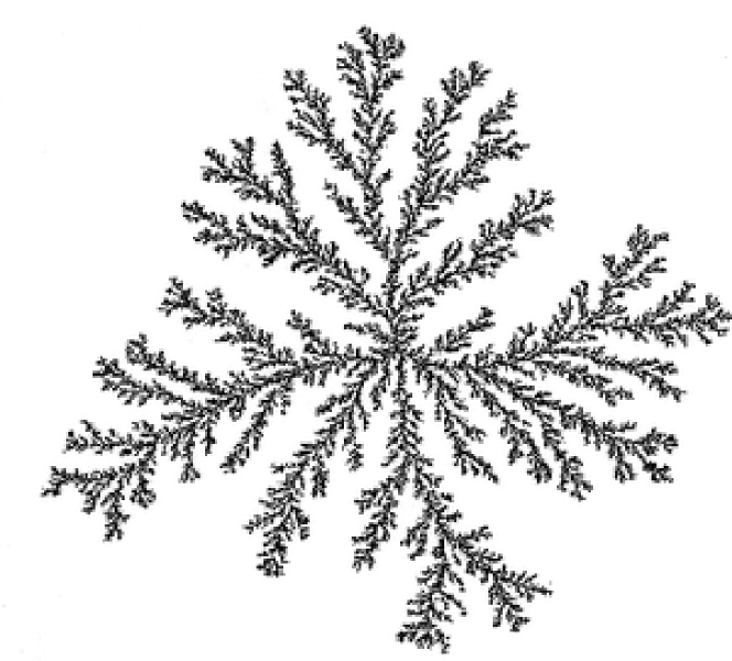
Figure 38: An exemple of cluster obtained by iterating conformal maps. Notice the similarity with the DLA sample of Fig.19.

One starts with an elementary map corresponding to the gluing of a tiny bump, of linear size $\lambda$, to the unit disk. A large variety of choices is possible, whose influence on the final structure of the domain is unclear. An example is given by the following formulæ ($g_{\lambda}$ is the inverse map of $f_{\lambda}$):

$$g_{\lambda}(z) = z\ \frac{z\cos\lambda-1}{z-\cos\lambda}$$

$$f_{\lambda}(w)= = (2\cos\lambda)^{-1}\left[{w+1+\sqrt{w^{2}-2w\cos 2\lambda+1}}\right]$$

where $f_{\lambda}$ correspond to the deformation of the unit disk obtained by gluing a semi-disk centered at point $1$ and whose two intersecting points with the unit circle define a cone of angle $2\lambda$. For $\lambda\ll 1$, the area of the added bump is of order $\lambda^{2}$. But other choices are possible and have been used [40, 73].

Gluing a bump around point $e^{i\theta}$ on the unit circle is obtained by rotating these maps. The uniformizing maps are then

$$f_{\lambda;\theta}(w)=e^{i\theta}\,f_{\lambda}(we^{-i\theta})$$

The growth of the domain is obtained by successively iterating the maps $f_{\lambda_{n};\theta_{n}}$ with various values for the size $\lambda_{n}$ and the position $\theta_{n}$ of the bumps. See Fig.39. Namely, if after $n$ iterations the complement of the unit disk is uniformized into the complement of the domain by the map $F_{(n)}(w)$, then at the next $(n+1)^{\rm th}$ iteration the uniformizing map is given by:

$$F_{(n+1)}(w)=F_{(n)}(\,f_{\lambda_{n+1};\theta_{n+1}}(w)\,)$$ (76)

For the inverse maps, this becomes $G_{(n+1)}=g_{\lambda_{n+1};\theta_{n+1}}\circ G_{(n)}$.

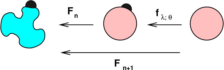
Figure 39: Iteration of conformal maps.

To fully define the model one has to specify the choice of the parameter $\lambda_{n}$ and $\theta_{n}$ at each iteration. Since $\lambda_{n}$ codes for the linear size of the added bump and since locally conformal maps act as dilatations, the usual choice is to rescale $\lambda_{n+1}$ by a power of $|F_{(n)}^{\prime}(e^{i\theta_{n}})|$ as:

$$\lambda_{n+1}=\lambda_{0}\ |F_{(n)}^{\prime}(e^{i\theta_{n}})|^{-\alpha/2},\quad 0\leq\alpha\leq 2$$

The case $\alpha=2$ corresponds to DLA as the physical area of the added bump are approximatively constant and equal to $\lambda_{0}$ at each iterations. In the other case, the area of the added bump scales as $|F_{(n)}^{\prime}(e^{i\theta_{n}})|^{2-\alpha}$.

The positions of the added bump are usually taken uniformly distributed on the mathematical unit circle with a measure $d\theta/2\pi$.

It is clear that this discrete model with $\alpha=2$ provides a regularization of Laplacian growth with $\lambda_{0}$ playing the role of an ultraviolet cutoff. This may also be seen by looking at the naive limit of a small cutoff. Indeed, a naive expansion as $\lambda_{n}\ll 1$ gives that $F_{(n+1)}=F_{(n)}+\delta F_{(n)}$ with

$$\delta F_{(n)}(w)\simeq\lambda_{n}\,wF_{(n)}^{\prime}(w)\,\left(\frac{w+e^{i\theta_{n}}}{w-e^{i\theta_{n}}}\right)$$

where we used the expression of $f_{\lambda}$ for $\lambda\ll 1$. Using the recursive expression for $\lambda_{n}$ and averaging over $\theta$ with a uniform distribution yields:

$$\langle\delta F(w)\rangle=\lambda_{0}\,wF^{\prime}(w)\,\oint\frac{d\theta}{2\pi}|F^{\prime}(e^{i\theta})|^{-\alpha}\,\frac{w+e^{i\theta}}{w-e^{i\theta}}$$

For $\alpha=2$ this reproduces the Loewner chain for Laplacian growth. But this computation is too naive as the small cutoff limit is not smooth, a fact which is at the origin of the non trivial fractal dimensions of the growing domains.

There are only very few mathematical results on these discrete models. The most recent one [116] deals with the simplest (yet interesting but not very physical) model with $\alpha=0$. It proves the convergence of the iteration to well-defined random maps uniformizing domains of Hausdorff dimension $1$. However, these models have been studied numerically extensively. There exists a huge literature on this subject but see ref.[40, 73] for instance. These studies confirm that the fractal dimension of DLA clusters with $\alpha=2$ is $D_{\rm dla}\simeq 1.71$ but they also provide further informations on the harmonic measure multi-fractal spectrum. Results on the $\alpha$ dependence of the fractal dimension may be found eg. in ref.[70].

Various generalizations have been introduced. For instance, in ref.[72] a model of iterated conformal maps has been defined in which particles are not added one by one but by layers. These models have one control parameter coding for the degree of coverage of the layer at each iterative step. By varying this parameter the model interpolates between discrete DLA and a discrete version of the Hele-Shaw problem. The fractal dimension of the resulting clusters varies with this parameter [5].

8.5 Miscellaneous

DLA and Laplacian growth have a large domain of applicability since they are based on simple Brownian diffusion, and a large number of works have devoted to them. See [22, 65, 68, 18, 130] for reviews. But precise – and mathematically clean – descriptions are unknown. In particular it is yet not clear whether these descriptions are universal or not, and numerical simulations point in different directions. Indeed, Laplacian growth has to be regularized and, as we discussed, there are different ways to regularize it – DLA, the Hele-Shaw problem, the discrete iterations provide different regularizations. Each of them involve an ultraviolet cut-off, and it is yet not clear whether the singular limits of vanishingly small cut-off are identical. If it is, then universality holds. It is tempting to suppose that a renormalization group inspired approach should provide a way to answer this question.

Finally, it will be interesting to extend the previous considerations to fracture related problems, see eg. [75].

Acknowledgements:

We benefited from discussions with many of our colleagues. We would like to thank especially Vincent Beffara, John Cardy, Antti Kupiainen, Kalle Kytölä, Greg Lawler, Vincent Pasquier, Wendelin Werner and Paul Wiegmann.

Work supported in part by EC contract number HPRN-CT-2002-00325 of the EUCLID research training network, and in part by EC contract number MRTN-CT-2004-5652 of the ENIGMA research training network.

Appendix A Probabilistic background

We summarize here some of the basics tools of probability theory with the aim of filling part of the gap between the mathematic and physics languages.

A.1 Tribes and measurable spaces

If $\Omega$ is any set, a tribe (or $\sigma$-algebra) on $\Omega$ is a subset of $2^{\Omega}$ which contains $\Omega$, is stable by complementation and by denumerable unions. Thus ${\mathcal{F}}\subset 2^{\Omega}$ is a tribe on $\Omega$ if

– i) $\Omega\in{\mathcal{F}}$,
– ii) if $A\in{\mathcal{F}}$ its complement $A^{c}\in{\mathcal{F}}$,
– iii) if $A_{n}\in{\mathcal{F}}$ for $n\in{\mathbb{N}}$ then $\cup_{n}A_{n}\in{\mathcal{F}}$.
Two trivial examples are ${\mathcal{F}}=\{\Omega,\emptyset\}$, the trivial tribe, and ${\mathcal{F}}=2^{\Omega}$, the total tribe. Because of ii), iii) can be replaced by
– $\textit{iii}^{\prime}$) if $A_{n}\in{\mathcal{F}}$ for $n\in{\mathbb{N}}$ then $\cap_{n}A_{n}\in{\mathcal{F}}$,
i.e. by stability under denumerable intersections.

An arbitrary intersection of tribes is still a tribe. An arbitrary subset ${\mathcal{S}}\subset 2^{\Omega}$ is contained in a smallest tribe denoted by $\sigma({\mathcal{S}})$, the intersection of all tribes containing ${\mathcal{S}}$. If $\Omega$ is a topological space, the smallest tribe containing the open sets is called the Borel tribe, usually denoted by ${\mathcal{B}}$.

The pair $(\Omega,{\mathcal{F}})$ is usually refered as a measurable space. A map $f$ from a measurable space $(\Omega,{\mathcal{F}})$ to another measurable space $(\Omega^{\prime},{\mathcal{F}}^{\prime})$ is called measurable if $f^{-1}(A^{\prime})\in{\mathcal{F}}$ whenever $A^{\prime}\in{\mathcal{F}}^{\prime}$.

Example 1

: coin tossing.

Think for example of a simple model of a coin tossing game. Games of length $n\geq 1$ can be modeled to take place in the space $\Omega_{n}\equiv\{-1,1\}^{[1,n]}$, where $1$ stands for “head” say, and $-1$ for “tail”. Thus $\Omega_{n}$ is made of finite sequences $X_{1},\cdots,X_{n}$ with values in $\pm 1$. Infinite games take place in $\Omega\equiv\{-1,1\}^{{\mathbb{N}}^{*}}$, which is made of infinite sequences $X_{1},X_{2},\cdots$. Troncation after the $n^{th}$ term gives a map $\pi_{n}$ from $\Omega$ onto $\Omega_{n}$ for each $n\geq 1$. For each $n$ $2^{\Omega_{n}}$ is a tribe on $\Omega_{n}$ and ${\mathcal{F}}_{n}=\{\pi_{n}^{-1}(A),A\in 2^{\Omega_{n}}\}$ is a tribe for $\Omega$, which conveys intuitively the knowledge of what happens in the first $n$ toses of the coin. Clearly ${\mathcal{F}}_{1}\subset{\mathcal{F}}_{2}\subset\cdots$ is an increasing sequence of tribes. The smallest tribe containing all of them, denoted by ${\mathcal{F}}$, is larger than the union $\cup_{n}{\mathcal{F}}_{n}$ (which is not a tribe !). The subset of $\Omega$ made of sequences in which $1$ appears at least once is in ${\mathcal{F}}$, but in no ${\mathcal{F}}_{n}$. The same is true of $\{\omega\in\Omega,S_{n}(\omega)/n\;\mathrm{converges}\}$ where $S_{n}$ is the sum of the first $n$ steps, $S_{n}\equiv X_{1}+\cdots+X_{n}$. One way to see it is to write this set as $\cap_{k=1}^{\infty}\cup_{l=1}^{\infty}\cap_{n>m>l}A_{k,m,n}$ where

$$A_{k,m,n}\equiv\left\{\omega\in\Omega,\left|\frac{S_{n}(\omega)}{n}-\frac{S_{m}(\omega)}{m}\right|<\frac{1}{k}\right\}\in{\mathcal{F}}_{n}.$$

In probability theory, the members of ${\mathcal{F}}$ are assigned probabilities in a consistent way (see below), and consistency is one among many of the reasons to consider other tribes than the total tribe (see the coin tossing example to find other reasons).

The statistical mechanics viewpoint.

Let us explain now why tribes remain most of the time behind the scene in statistical mechanics.

In statistical mechanics, the configuration space $\Omega$ is often finite (think for example of Ising variables on a finite number of sites) or sometimes denumerable (as in height models) to start with. Then ${\mathcal{F}}=2^{\Omega}$ will turn out to be a consistent choice. Taking the thermodynamic limit is in general a nontrivial step from the point of view of probability theory, but the difficulties are most of the time of technical nature, and do not need to be adressed carefull by physicists to get the correct answer to the questions they are interested in.

If $\Omega$ is finite or countable and ${\mathcal{F}}$ is a tribe, it is not difficult to show that there is a finite or countable index set $I$ and a partition of $\Omega=\cup_{i\in I}\Omega_{i}$ such that the members of ${\mathcal{F}}$ are the unions $\cup_{j\in J}\Omega_{j}$ when $J$ runs over the subsets of $I$, i.e. ${\mathcal{F}}$ is the smallest tribe containing all the sets of the partition. The $\Omega_{i}$’s are just the minimal elements of ${\mathcal{F}}$ for the inclusion. We say that $\Omega=\cup_{i\in I}\Omega_{i}$ is the partition associated to ${\mathcal{F}}$.

Hence in the context of finite or countable configuration spaces, there is an equivalence between tribes and partitions. Partitions are the standard approach of statistical mechanics. An archetypal example in these notes is to partition $\Omega$ according to the position of (the beginning of) an interface.

A.2 Probability spaces and random variables

A measure space is a triple $(\Omega,{\mathcal{F}},\mu)$ where ${\mathcal{F}}$ is a tribe on $\Omega$ and $\mu$ a map from ${\mathcal{F}}$ to $[0,+\infty]$ such that if $A_{n}$, $n\in\mathbb{N}$ is a sequence of disjoint members of ${\mathcal{F}}$ and $A=\cup_{n}A_{n}$ then $\mu(A)=\sum_{n}\mu(A_{n})$ ($\mu$ is said to be countably additive).

Among measure spaces, probability spaces are most important in these notes, a notable exception being Poisson random measures to be defined below.

A measure space $(\Omega,{\mathcal{F}},p)$ is a probability space if $p(\Omega)=1$.

If $(\Omega,{\mathcal{F}},p)$ is a probability space and $(\Omega^{\prime},{\mathcal{F}}^{\prime})$ a measurable space, a random variable $X$ on $(\Omega,{\mathcal{F}},p)$ with values $(\Omega^{\prime},{\mathcal{F}}^{\prime})$ is simply a measurable map from $(\Omega,{\mathcal{F}})$ to $(\Omega^{\prime},{\mathcal{F}}^{\prime})$. Quite often, random variables take values in ${\mathbb{R}}$ endowed with the Borel tribe.

An arbitrary collection of random variables on $(\Omega,{\mathcal{F}},p)$ (with possibly different target spaces) generates a subtribe of ${\mathcal{F}}$, namely the smallest tribe for which all random variables in the collection are measurable.

A random variable $X$ induces a probability $p_{X}$ on its target space $(\Omega^{\prime},{\mathcal{F}}^{\prime})$ by $p_{X}(A^{\prime})\equiv p(X^{-1}(A^{\prime}))$, for which the notation $p(X\in A^{\prime})$ is also intuitively appealing. This induced probability is called the probability distribution of $X$.

Example 2

: Poisson distribution.

Fix $\lambda\in[0,+\infty[$, take $\Omega=\{0,1,\cdots\}$, ${\mathcal{F}}=2^{\Omega}$ and, for $A\in\Omega$, $p(A)=e^{-\lambda}\sum_{n\in A}\frac{\lambda^{n}}{n!}$. It is immediate that $(\Omega,{\mathcal{F}},p)$ is a probability space. A slight extension is when $X$ is a random variable on a probability space $(\Omega,{\mathcal{F}},p)$ with values in $\{0,1,\cdots\}$ and probability distribution as above. This distribution is called the Poisson distribution of parameter $\lambda$.

Whenever $\Omega$ is not countable, probability distributions are usually defined by specifying probabilities of a simple subclass ${\mathcal{S}}$ of ${\mathcal{F}}$ such that ${\mathcal{F}}=\sigma({\mathcal{S}})$, and using an extension theorem to get a probability defined on all of ${\mathcal{F}}$. Doing it by hand for a special case is painful. The extension theorems work when some consistency condition holds for the probabilities specified on ${\mathcal{S}}$. The reader can look at example 3 and refer to the litterature for more details.

Example 3

: Fair coin tossing.

Take $\Omega\equiv\{-1,1\}^{{\mathbb{N}}^{*}}$ with tribe ${\mathcal{F}}=\sigma(\cup_{n}{\mathcal{F}}_{n})$. Each element $\omega$ of $\Omega$ is an infinite sequence $X_{1},X_{2},\cdots$, which we can write in a tautological way $X_{1}(\omega),X_{2}(\omega),\cdots$ and the coordinate maps $\omega\mapsto X_{n}(\omega)$ are measurable for $n=1,2,\cdots$. By construction, ${\mathcal{F}}_{n}$ is the smallest tribe making $X_{1},\cdots,X_{n}$ measurable.

Define a probability $p_{n}$ on ${\mathcal{F}}_{n}$ by $p_{n}(A)=|\pi_{n}(A)|/2^{n}$ for $A\in{\mathcal{F}}_{n}$ (recall that $\pi_{n}(A)$ is a subset of $\Omega_{n}$ and $|\Omega_{n}|=2^{n}$).

The probabilities $p_{n}$ are consistent in the following way : if $A\in{\mathcal{F}}_{m}$ and $n\geq m$ then $A\in{\mathcal{F}}_{m}$ and $p_{n}(A)=p_{m}(A)$. So we can assemble the $p_{n}$’s into a function $p$ on ${\mathcal{S}}\equiv\cup_{n}{\mathcal{F}}_{n}$.

If $A_{k}$ is a sequence of disjoint elements of ${\mathcal{S}}$ such that $\cup_{k}A_{k}$ is again in ${\mathcal{S}}$, then $p(\cup_{k}A_{k})=\sum_{k}p(A_{k})$. The proof is simple if tedious. This condition is enough to garanty a consistent extension of $p$ to a probability on ${\mathcal{F}}=\sigma({\mathcal{S}})$. This is one of the useful extension theorems in the field.

Example 4

: The uniform distribution.

Take $\Omega=[0,1]$ with the Borel tribe ${\mathcal{B}}$. Le length $b-a$ of an open interval $]a,b[$, $0\leq a<b\leq 1$, can be extended in a unique way to a probability measure on $(\Omega,{\mathcal{B}})$, called the uniform distribution, which is nothing but the well-known Lebesgue measure.

Consider the map $f$ from $\{-1,1\}^{{\mathbb{N}}^{*}}$ to $[0,1]$ defined by $f(X_{1},X_{2},\cdots)=\sum_{n>0}b_{n}/2^{n},$ where $b_{n}\equiv(X_{n}+1)/2\in\{0,1\}$ The sequence $(b_{1},b_{2},\cdots)$ is simply the binary expansion of the real number $f(X_{1},X_{2},\cdots)$. As a consequence, this map is such that if $A\in\cup_{n}{\mathcal{F}}_{n}$, the image $f(A)$ is a finite union of closed intervals and the Lebesgue measure of $f(A)$ coincides with $p(A)$. This indicates that from a probabilistic viewpoint $([0,1],{\mathcal{B}},dx)$ and $(\{-1,1\}^{{\mathbb{N}}^{*}},{\mathcal{F}},p)$ are essentially indistiguishable. In fact, one can show that $(\{-1,1\}^{{\mathbb{N}}^{*}},{\mathcal{F}},p)$ is in some precise sense equivalent as a probability space to any nondenumerable probability space. Let us give two modest illustrations. If $d\geq 2$ is and integer, on can by split a sequence $X=(X_{1},X_{2},\cdots)$ in $d$ sequences, $X^{(1)}=(X_{1},X_{d+1},X_{2d+1},\cdots),\cdots,X^{(d)}=(X_{d},X_{2d},X_{3d},\cdots)$ to show quickly that $([0,1],{\mathcal{B}},dx)$ and $([0,1]^{d},{\mathcal{B}},d^{d}x)$ are one and the same probability space. One can also split a sequence $X=(X_{1},X_{2},\cdots)$ into a denumerable family of sequences $X^{(1)}=(X_{1},X_{3},X_{5},\cdots),X^{(2)}=(X_{2},X_{6},X_{10},\cdots),X^{(3)}=(X_{4},X_{12},X_{20},\cdots),\cdots$, a fact Wiener used for its original definition of Brownian motion (see below).

Example 5

: The Gaussian distribution.

Take $\Omega={\mathbb{R}}$ with the Borel tribe ${\mathcal{B}}$, and define $p(A)=\int_{A}\frac{dx}{\sqrt{2\pi}}e^{-x^{2}/2}\equiv\int{\mathbf{1}}_{A}\frac{dx}{\sqrt{2\pi}}e^{-x^{2}/2}$ for $A\in{\mathcal{B}}$. This is the standard Gaussian distribution. If $X$ is a random variable which is either constant or such that $(X-b)/a$ follows the standard Gaussian distribution for some real numbers $a\neq 0$ and $b$, $X$ is called a Gaussian random variable. When $b=0$, $X$ is called a centered Gaussian random variable.

If $X_{1},\cdots,X_{n}$ are real random variables, the vector $(X_{1},\cdots,X_{n})$ is called Gaussian if any linear combination $\sum_{i}c_{i}X_{i}$ is a Gaussian random variable.

For instance, if $(U,V)$ is uniformly distributed in the unit square $[0,1]^{2}$, one can check that $(\log U\cos 2\pi V,\log U\sin 2\pi V)$ is a Gaussian vector. In fact the two components are independent standard Gaussian random variables. Combining this with our remarks on the ”size” of the probability space of fair coin tossing, one sees that it can accomodate a countable family of independent standard Gaussian random variables.

The statistical mechanics viewpoint.

In statistical mechanics, an energy function $E$ on the (finite or denumerable) space $\Omega$ is given, and there is a simple formula for the relative probability of $\omega$ and $\omega^{\prime}$ at temperature $T=1/\beta$:

$$p(\omega)/p(\omega^{\prime})=e^{\beta(E(\omega^{\prime})-E(\omega))}.$$

The partition function $Z=\sum_{\omega\in\Omega}e^{-\beta E(\omega)}$ gives the normalization of the probability. If $Z<+\infty$, this defines a probability on $(\Omega,2^{\Omega})$.

A real random variable is any function from $\Omega$ to ${\mathbb{R}}$, also called an observable. If we look at another tribe ${\mathcal{F}}$ with associated partition $\Omega=\cup_{i\in I}\Omega_{i}$, a random variable for $(\Omega,{\mathcal{F}})$ is a function from $\Omega$ to ${\mathbb{R}}$ constant on each $\Omega_{i}$.

A.3 (Conditional) expectations

Let $(\Omega,{\mathcal{F}},p)$ be a probability space.

Finite sums and products of random variables with values in $(\mathbb{R},{\mathcal{B}})$ are again random variables. A useful quantity associated to a real random variable is its average, usually called expectation in the probabilistic context. It is defined at first only for so called simple random variables, those which can be written as $X=\sum_{i=1}^{n}x_{i}{\mathbf{1}}_{A_{i}}$ for some integer $n$, real numbers $x_{i}$ and measurable sets $A_{i}\in{\mathcal{F}}$ for $i=1,\cdots,n$. This decomposition is in general not unique, but the expectation, defined by ${\mathbf{E}}\left[X\right]\equiv\sum_{i=1}^{n}x_{i}p(A_{i})$ can be shown to be well defined. If $\Omega$ is finite, every random variables is simple. In the other cases, one tries to approximate more general random variables by simple ones, and define the expectation by a limiting procedure. For instance, if $\Omega$ is countable, then any tribe ${\mathcal{F}}$ is the smallest tribe containing all sets of a certain partition $\Omega=\cup_{i\in I}\Omega_{i}$ into a finite or countable number of pieces. The most general random variable can uniquely be written $X=\sum_{i\in I}x_{i}{\mathbf{1}}_{\Omega_{i}}$. The limiting procedure allows to define the expectation of $X$ under the condition $\sum_{i\in I}|x_{i}|p(\Omega_{i})<\infty$ by the formula ${\mathbf{E}}\left[X\right]\equiv\sum_{i\in I}x_{i}p(\Omega_{i})$, a formula wich could also be taken as a definition in this simple case. In the general case, an expectation with values in $[0,+\infty]$ can be defined for any positive random variable, and ${\mathbf{E}}\left[X\right]$ can be defined if ${\mathbf{E}}\left[|X|\right]<+\infty$.

The statistical mechanics viewpoint.

If $\Omega$ is countable, we can consider the tribe ${\mathcal{F}}=2^{\Omega}$. A real random variable, or observable, is a function $X$ from $\Omega$ to ${\mathbb{R}}$ and

$${\mathbf{E}}\left[X\right]\equiv\left<X\right>\equiv\frac{1}{Z}\sum_{\omega\in\Omega}X(\omega)e^{-\beta E(\omega)},$$

whenever the sum is absolutely convergent.

The reader is probably familiar with the notion of conditional probability : if $(\Omega,{\mathcal{F}},p)$ is a probability space, $A,B\in{\mathcal{F}}$ and $p(B)\neq 0$ the probability of $A$ given that $B$ occurs (or simply the probability of $A$ given $B$) is defined to be $p(A|B)\equiv p(A\cap B)/p(B)$. The events $A$ and $B$ are called independent if $p(A\cap B)=p(A)p(B)$ and then $p(A|B)=p(A)$. Hence conditional probabilities and independence convey the correct intuitive meaning.

Independence can be formulated at different levels. The events of a family $\{A_{\alpha},\alpha\in I\}$ are called independent if $p(\cap_{J}A_{\alpha})=\prod_{J}p(A_{\alpha})$ for any finite subset $J$ of $I$. The tribes $\{{\mathcal{F}}_{\alpha},\alpha\in I\}$ are called independent if the events $\{A_{\alpha},\alpha\in I\}$ are independent whenever $A_{\alpha}\in{\mathcal{F}}_{\alpha}$ for all $\alpha$’s in $I$. The random variables $\{X_{\alpha},\alpha\in I\}$ are called independent if the tribes $\sigma(X_{\alpha})$ they generate are independent. If moreover the functions $\{f_{\alpha},\alpha\in I\}$ are measurable functions from $\mathbb{R}$ to $\mathbb{R}$ such that ${\mathbf{E}}\left[|f_{\alpha}(X_{\alpha})|\right]<+\infty$ for $\alpha\in I$ and $J$ is a finite subset of $I$, then ${\mathbf{E}}\left[(\prod_{J}f_{\alpha}(X_{\alpha}))\right]=\prod_{J}{\mathbf{E}}\left[(f_{\alpha}(X_{\alpha}))\right]$. Conversely, this multiplicative property for all measurable functions from $\mathbb{R}$ to $\mathbb{R}$ such that ${\mathbf{E}}\left[|f_{\alpha}(X_{\alpha})|\right]<+\infty$ for $\alpha\in I$ ensures that the random variables $\{X_{\alpha},\alpha\in I\}$ are independant. This is easy to check for simple random variables.

Example 6

: The Kolmogorov strong law of large numbers.

Let $X_{n}$, $n=1,2,\cdots$ is a sequence of real independant identically distributed random variables on $(\Omega,{\mathcal{F}},p)$ with partial sums $S_{n}=X_{1}+\cdots,X_{n}$, $n\geq 1$.

– If ${\mathbf{E}}\left[|X_{n}|\right]<+\infty$ and ${\mathbf{E}}\left[X_{n}\right]=\mu$, the sequence $S_{n}/n$ converges to $\mu$ almost surely (i.e. the subset of $\Omega$ such that $S_{n}/n$ does not converges to $\mu$ fits into elements of ${\mathcal{F}}$ of arbitrary small probability).

– If ${\mathbf{E}}\left[|X_{n}|\right]=+\infty$, the sequence $S_{n}/n$ diverges almost surely.

Example 7

: Poisson random measures.

If $(\Omega,{\mathcal{F}},\mu)$ is a measure space and ${\mathcal{F}}_{0}\equiv\{B\in{\mathcal{F}}\;|\;\mu(B)<\infty\}$ there exits a collection of integer valued random variables $\{N_{B}\;|B\in{\mathcal{F}}_{0}\}$ such that

– i) $N_{B}$ is a Poisson random variable with mean $\mu(B)$,

– ii) if $B_{1},\cdots,B_{n}\in{\mathcal{F}}_{0}$ are disjoint, the variables $N_{B_{1}},\cdots,N_{B_{n}}$ are independent,

– iii) if $B,B^{\prime}\in{\mathcal{F}}_{0}$, $Cov(N_{B},N_{B^{\prime}})\equiv{\mathbf{E}}\left[N_{B}N_{B^{\prime}}\right]-{\mathbf{E}}\left[N_{B}\right]{\mathbf{E}}\left[N_{B^{\prime}}\right]=\mu(B\cap B^{\prime})$.
This collection is called the Poisson random measure on $(\Omega,{\mathcal{F}},\mu)$. Intuitively, a sample is a collection of points in $\Omega$, the random variables $N_{B}$ describe the number of points in region $B$, which follows a Poisson distribution. Disjoint regions are idependent. Conditions i), ii), iii) ensure that the number of points in a disjoint union is (almost surely) the sum of the numbers of points in each separate region.

This notions of expectations and conditional probabilities are combined in a very useful way in the concept of conditional expectation.

Let $X$ be an ${\mathcal{F}}$ random variable with ${\mathbf{E}}\left[|X|\right]<+\infty$ and ${\mathcal{F}}^{\prime}$ be a subtribe of ${\mathcal{F}}$. A conditional expectation of $X$ given ${\mathcal{F}}^{\prime}$ is an ${\mathcal{F}}^{\prime}$ measurable random variable $Y$such that ${\mathbf{E}}\left[|Y|\right]<+\infty$ and

$${\mathbf{E}}\left[X{\mathbf{1}}_{A}\right]={\mathbf{E}}\left[Y{\mathbf{1}}_{A}\right]$$

for any $A\in{\mathcal{F}}^{\prime}$. The notation $Y={\mathbf{E}}\left[X|{\mathcal{F}}^{\prime}\right]$ is standard. Let us stress that ${\mathbf{E}}\left[X|{\mathcal{F}}^{\prime}\right]$ is by definition ${\mathcal{F}}^{\prime}$ measurable. The above definition is not a constructive, but it turns out to be a characterization which is most useful to work with conditional expectations. The general abstract argument for the existence of a conditional expectation ${\mathbf{E}}\left[X|{\mathcal{F}}^{\prime}\right]$ relies on the Radon Nykodim theorem or on projections in Hilbert spaces of square integrable random variables, i.e. on cornerstones of measure theory (see [50]).

Note that if $X$ is ${\mathcal{F}}^{\prime}$ measurable, then $X$ itself satisfies the properties of ${\mathbf{E}}\left[X|{\mathcal{F}}^{\prime}\right]$. One can also see that if ${\mathcal{F}}^{\prime\prime}$ is a subtribe of ${\mathcal{F}}^{\prime}$,

$${\mathbf{E}}\left[{\mathbf{E}}\left[X|{\mathcal{F}}^{\prime}\right]|{\mathcal{F}}^{\prime\prime}\right]={\mathbf{E}}\left[{\mathbf{E}}\left[X|{\mathcal{F}}^{\prime\prime}\right]|{\mathcal{F}}^{\prime}\right]={\mathbf{E}}\left[X|{\mathcal{F}}^{\prime\prime}\right].$$

Thus, when conditional expectations are nested, the smallest tribe wins.

More modestly, we construct conditional expectations in the case when $\Omega$ is finite or countable, so that ${\mathcal{F}}$ is associated to a finite or countable partition $\Omega=\cup_{i\in I}\Omega_{i}$. Suppose that ${\mathcal{F}}^{\prime}$ is a subtribe of ${\mathcal{F}}$. Then $I$ can be partitionned into a finite or countable number of pieces $I=\cup_{j\in J}I_{j}$ in such a way that ${\mathcal{F}}^{\prime}$ is the smallest tribe containing all $\Omega^{\prime}_{j}\equiv\cup_{i\in I_{j}}\Omega_{i}$. If $X=\sum_{i\in I}x_{i}{\mathbf{1}}_{\Omega_{i}}$ is a random variable with expectation (i.e. $\sum_{i\in I}|x_{i}|p(\Omega_{i})<\infty$ as above), and $X^{\prime}=\sum_{j\in J}x^{\prime}_{j}{\mathbf{1}}_{\Omega^{\prime}_{j}}$ is an ${\mathcal{F}}^{\prime}$ measurable random variable, ${\mathbf{E}}\left[X{\mathbf{1}}_{\Omega^{\prime}_{j}}\right]={\mathbf{E}}\left[X^{\prime}{\mathbf{1}}_{\Omega^{\prime}_{j}}\right]$ says that $p(\Omega^{\prime}_{j})x^{\prime}_{j}\equiv\sum_{i\in I_{j}}x_{i}p(\Omega_{i})$. As $p(\Omega^{\prime}_{j})=\sum_{i\in I_{j}}p(\Omega_{i})$, this formula fixes $x^{\prime}_{j}$ if $p(\Omega^{\prime}_{j})\neq 0$ but leaves the value of $x^{\prime}_{j}$ undetermined if $p(\Omega^{\prime}_{j})=0$. Then, for any choice of the $x^{\prime}_{j}$ satisfying the above conditions and , for $A\in{\mathcal{F}}^{\prime}$, ${\mathbf{E}}\left[X{\mathbf{1}}_{A^{\prime}}\right]={\mathbf{E}}\left[X^{\prime}{\mathbf{1}}_{A^{\prime}}\right]$, i.e. $X^{\prime}$ is a conditional expectation of $X$ given ${\mathcal{F}}^{\prime}$. So conditional expectations exist, in general they form a class of ${\mathcal{F}}^{\prime}$-measurable random variables that coincide except on a set of probability $0$.

The statistical mechanics viewpoint.

In statistical mechanics, the starting point is not absolute probabilities, but relative probabilities. This implies the use of partition functions, and trivializes the notion of conditional expectations, in that physicists manipulate them all the time without ever giving them a special name.

If $\Omega$ is countable, we can consider the tribe ${\mathcal{F}}=2^{\Omega}$ associated with a partition of $\Omega$ into singletons. The context may dictate to split $\Omega$ in larger pieces. For instance, in the Ising model, we may compare different possible boundary conditions, and partition $\Omega$ accordingly. Or as in these notes, fix boundary conditions that imply the presence of an interface and partition the configuration space according to (part of) the position of the interface. As a last illustration in the context of the renormalization group, we may split $\Omega$ according to the value of the magnetization of blocks of spin. All these contexts lead to a partition $\Omega=\cup_{j\in J}\Omega^{\prime}_{j}$ with associated tribe ${\mathcal{F}}^{\prime}$, partial partition functions $Z_{j}=\sum_{\omega\in\Omega^{\prime}_{j}}e^{-\beta E(\omega)}$, and, if $X$ is any observable, partial averages

$$\left<X\right>_{j}\equiv\frac{1}{Z_{j}}\sum_{\omega\in\Omega^{\prime}_{j}}X(\omega)e^{-\beta E(\omega)}.$$

The random variable taking the constant value $\left<X\right>_{j}$ on $\Omega^{\prime}_{j}$ is nothing but the conditional expectation of $X$ given ${\mathcal{F}}^{\prime}$.

It should be clear from the examples that conditional expectations are a general framework for all situations when one want to concentrate on certain degrees of freedom and average over the others. In some sense, the statistical mechanics framework is the most symmetrical, in that absolute probabilities are only a secondary concept, so that conditioning is transparent. Except for the special role played by the temperature which in principle appears in the Boltmann weight but not in the energy function, nothing indicates that $\Omega$ itself and the associated Boltzmann weights have not been obtained by a previous conditioning.

A.4 Martingales and stopping times : discrete setting

If $(\Omega,{\mathcal{F}},p)$ is a probability space, an increasing sequence ${\mathcal{F}}_{n},n=0,1,2,\cdots$ of subtribes of ${\mathcal{F}}$ is called a filtration. A sequence of random variables is also called a (random or stochastic) process. Most often, the target is the same, for all terms in the sequence. If the target is ${\mathbb{R}}$ one talks of a real process.

Given such a filtration,

– a sequence of random variables $A_{n},n=0,1,2,\cdots$ is adapted if $A_{n}$ is ${\mathcal{F}}_{n}$ measurable for each $n$.

– a real adapted process $M_{n},n=0,1,2,\cdots$ is a martingale if ${\mathbf{E}}\left[|M_{n}|\right]<\infty$ for each $n$ and ${\mathbf{E}}\left[M_{n}|{\mathcal{F}}_{m}\right]=M_{m}$ for $0<m<n$. Note that this condition by itself implies that the sequence $M_{n}$ is adapted, but for the problem that conditional expectations have ambiguities (on sets of measure zero).

– a real random variable $T$ with values in $0,1,2,\cdots,+\infty$ is said to be a stopping time if the event $T\leq n$ is in ${\mathcal{F}}_{n}$ for each $n$, or equivalently (in this discrete setting) if the event $T=n$ is in ${\mathcal{F}}_{n}$ for each $n$. It is an exercise to show that ${\mathcal{F}}_{T}\equiv\{A\in{\mathcal{F}}:A\cap\{T\leq n\}\in{\mathcal{F}}_{n}\;\mathrm{for}\;\mathrm{each}\;n\}$ is a tribe that summarizes the information ”collected up to $T$”.

One should view the parameter $n$ as a discrete time, ${\mathcal{F}}_{n}$ as the knowlege accumulated up to time $n$. An adapted sequence is one whose description at time $n$ does not require knowledge of the future. A martingale is such that its expectation in the future given the knowledge accumulated up to now is its present value. A stopping time is a random time for which the present knowledge is enough to decide if it has occurred in the past. Note that if $h$ is an increasing map from $\mathbb{N}$ to $\mathbb{N}$ and $X_{n}$ is adapted (resp. a martingale) for ${\mathcal{F}}_{n}$, then $X_{h(n)}$ is adapted (resp. a martingale) for the filtration ${\mathcal{F}}_{h(n)}$.

From the general rule of nesting of expectations, ${\mathbb{E}}M_{n}={\mathbf{E}}\left[{\mathbf{E}}\left[M_{n}|{\mathcal{F}}_{0}\right]\right]$, so if the sequence $M_{n}$ is a martingale, ${\mathbf{E}}\left[M_{n}\right]={\mathbf{E}}\left[M_{0}\right]$ : martingales are time independant in average.

If $X_{n}$ is a sequence of random variables and $N$ is a real random variable with values in $0,1,2,\cdots$, one can construct a new random variable $X_{N}$ by setting $X_{N}(\omega)\equiv X_{N(\omega)}(\omega)$ for $\omega\in\Omega$ , or equivalently, $X_{N}=\sum_{n}X_{n}{\mathbf{1}}_{N=n}$.

Part of the usefulness of martingales comes from the following : if $M_{n},n=0,1,2,\cdots$ is a martingale, and $T$ is a bounded stopping time (i.e. there is an integer $m$ such that $T$ takes values in $0,1,\cdots,m$), ${\mathbf{E}}\left[M_{T}\right]={\mathbf{E}}\left[M_{0}\right]$. The proof is simple and instructive. If $T\leq m$

$${\mathbf{E}}\left[M_{T}\right] = {\mathbf{E}}\left[\sum_{n=0}^{m}M_{n}{\mathbf{1}}_{T=n}\right]=\sum_{n=0}^{m}{\mathbf{E}}\left[M_{n}{\mathbf{1}}_{T=n}\right]$$

$$= \sum_{n=0}^{m}{\mathbf{E}}\left[{\mathbf{E}}\left[M_{m}|{\mathcal{F}}_{n}\right]{\mathbf{1}}_{T=n}\right]$$

$$= \sum_{n=0}^{m}{\mathbf{E}}\left[M_{m}{\mathbf{1}}_{T=n}\right]={\mathbf{E}}\left[M_{m}\sum_{n=0}^{m}{\mathbf{1}}_{T=n}\right]$$

$$= {\mathbf{E}}\left[M_{m}\right]={\mathbf{E}}\left[M_{0}\right].$$

The first equality is the definition of $M_{T}$, the third is the martingale property of the sequence $M_{n}$, the fourth is the definiting property of conditional expectations because ${\mathbf{1}}_{T=n}$ is ${\mathcal{F}}_{n}$ measurable. The other equalities are obvious.

This result can be adapted to deal with unbounded stopping times, as we shall see in applications.

Another use of martingales is that they allow to define new probability distributions. Suppose $M_{n}$ is a martingale such that $M_{0}=1$ and $M_{n}>0$ (with probability $1$) for $n\geq 0$. If $X$ is an ${\mathcal{F}}_{n}$ measurable random variable for some $n$, define $\tilde{\mathbf{E}}\left[X\right]\equiv{\mathbf{E}}\left[XM_{n}\right]$. This is a consistent definition because the martingale property ensures that $\tilde{\mathbf{E}}\left[XM_{n}\right]$ is the same for all $n$’s such that $X$ is ${\mathcal{F}}_{n}$ measurable. In the same spirit, If $A\in{\mathcal{F}}_{n}$, define $\tilde{p}(A)\equiv{\mathbf{E}}\left[{\mathbf{1}}_{A}M_{n}\right]$. This defines a consistent family of probability distribution on $(\Omega,{\mathcal{F}}_{n})$. Under technical growth conditions for $M_{n}$ in $n$ that we shall not try to make precise, $\tilde{p}$ extends to a probability measure on $(\Omega,\sigma(\{{\mathcal{F}}_{n}\})$. Note that this tribe may be strictly smaller than ${\mathcal{F}}$.

We start by illustrating these concepts for the simple random walk and then turn to statistical mechanics.

Example 8

: Martingales and fair coin tossing.

Recall $\Omega\equiv\{-1,1\}^{{\mathbb{N}}^{*}}$ is a space of infinite sequences $X_{1},X_{2},\cdots$. Set $S_{0}=0$ and $S_{n}=S_{n-1}+X_{n}=X_{1}+\cdots+X_{n}$ for $n\geq 1$. The tribe ${\mathcal{F}}_{n}$ is the smallest tribe making $X_{1},\cdots,X_{n}$ all measurable, and an ${\mathcal{F}}_{n}$ measurable random variable is simply an arbitrary function of $X_{1},\cdots,X_{n}$, defined on $\{-1,1\}^{n}$.

With the probability defined in 3, chosen to model intuitively independent tosses of a fair coin, the $X_{n}^{\prime}s$ are easily checked mathematically to be independent random variables, and ${\mathbf{E}}\left[X_{n}|{\mathcal{F}}_{m}\right]=0$ for $m<n$.

An adapted process is simply a sequence $A_{n}=f_{n}(X_{1},\cdots,X_{n})$ where $f_{n}$ is a function on $\{-1,1\}^{n}$. As $X_{n+1}^{2}=1$, the most general function of $X_{n+1}$ can be written in a unique way as $aX_{n+1}+b$. Hence, $f_{n+1}(X_{1},\cdots,X_{n},X_{n+1})-f_{n}(X_{1},\cdots,X_{n})$ can be written in a unique way as

$$f_{n+1}(X_{1},\cdots,X_{n},X_{n+1})-f_{n}(X_{1},\cdots,X_{n}) =$$

$$g_{n}(X_{1},\cdots,X_{n})X_{n+1}+h_{n}(X_{1},\cdots,X_{n})$$

More abstractly, any adapted process $A_{n}$ can be defined recursively in a unique way by a formula $A_{n+1}-A_{n}=B_{n}X_{n+1}+C_{n}$ where $B_{n}$ and $C_{n}$ are adapted processes. This leads us to the topic of stochastic difference equations.

Introducing the notation $\Delta U_{n}\equiv U_{n+1}-U_{n}$ for finite differences, we note that $\Delta S_{n}=X_{n+1}$ and $\Delta n=1$, so that the above equation can be rewritten $\Delta A_{n}=B_{n}\Delta S_{n}+C_{n}\Delta n$, which is equivalent to

$$A_{n}=A_{0}+\sum_{0}^{n-1}B_{m}\Delta S_{m}+\sum_{0}^{n-1}C_{m}\Delta m.$$

The second sum looks very much like a Riemann-Stiljes sum, but the first one is of another nature because $\Delta S_{m}$ oscillates. In the discrete setting, this is harmless, but a good version for continuous time requires the construction of a new integral, the Itô integral. Integrals are amenable objects mostly due to the change of variable formula and integration by parts. Let us look at their discrete counterparts. Suppose $k_{n}$ is a sequence of functions from $\mathbb{R}$ to $\mathbb{R}$ and look at the process $k_{n}(A_{n})$. The outcome is

$$\Delta k_{n}(A_{n})=B^{(k)}_{n}\Delta S_{n}+C^{(k)}_{n}\Delta n$$

where

$$B^{(k)}_{n}=\frac{k_{n+1}(A_{n}+B_{n}+C_{n})-k_{n+1}(A_{n}-B_{n}+C_{n})}{2},$$

which looks like a first order derivative, and

$$C^{(k)}_{n} = (k_{n+1}(A_{n}+C_{n})-k_{n}(A_{n}))$$

$$+ \frac{k_{n+1}(A_{n}+B_{n}+C_{n})-2k_{n+1}(A_{n}+C_{n})+k_{n+1}(A_{n}-B_{n}+C_{n})}{2}$$

which looks like the sum of a first derivative due to $\Delta n$ in the original equation and the explicit $n$ dependence in $k_{n}$, and a second derivative due to the oscillating nature of $\Delta S_{n}$ tamed by the fact that $(\Delta S_{n})^{2}=1$. We could pedantically call this the discrete Itô formula. The serious Itô formula relies heavily on a continuous time counterpart of $(\Delta S_{n})^{2}=1$. We shall come back to this later. For instance, if $\Delta A_{n}=\alpha A_{n}\Delta S_{n}$, one finds $\Delta\log A_{n}=\frac{1}{2}\log\frac{1+\alpha}{1-\alpha}\Delta S_{n}+\frac{1}{2}\log(1-\alpha^{2})\Delta n$, leading to $\log\frac{A_{n}}{A_{0}}=\frac{1}{2}\log\frac{1+\alpha}{1-\alpha}S_{n}+\frac{1}{2}\log(1-\alpha^{2})n$. In the same way, if $A^{(i)}_{n}$, $i=1,2$ are adapted processes, and $A_{n}=A^{(1)}_{n}A^{(2)}_{n}$, one finds that $\Delta A_{n}=B_{n}\Delta S_{n}+C_{n}\Delta n$ with $B_{n}=(A^{(1)}_{n}+C^{(1)}_{n})B^{(2)}_{n}+B^{(1)}_{n}(A^{(2)}_{n}+C^{(2)}_{n})$ and $C_{n}=A^{(1)}_{n}C^{(2)}_{n}+C^{(1)}_{n}A^{(2)}_{n}+B^{(1)}_{n}B^{(2)}_{n}$. For instance $\Delta S_{n}^{2}=2S_{n}\Delta S_{n}+\Delta n$.

Stochastic difference equations can be used in several ways. On the one hand, one can take $B_{n}$ and $C_{n}$ in full generality as given function of $X_{1},\cdots,X_{n}$. On the other hand, it causes no harm and can be very useful to add a dependence in $A_{1},\cdots,A_{n}$ in $B_{n}$ and $C_{n}$, because then the recursion relation itself ensures that indeed $B_{n}$, $C_{n}$ and $A_{n}$ are adapted. We shall give illustrations below. An important example is when $B_{n}$ and $C_{n}$ are given functions $b_{n}$ and $c_{n}$ of $A_{n}$, and $A_{n+1}-A_{n}=b_{n}(A_{n})X_{n+1}+c_{n}(A_{n})$. This defines an adapted Markov process which is called a diffusion.

In particular, ${\mathbb{E}}(A_{n+1}|{\mathcal{F}}_{n})=A_{n}+C_{n}$. So the process $A_{n}$ cannot be a martingale unless $C_{n}=0$, i.e. the process $C_{n}$ vanishes. The law for nesting conditional expectations (the smallest tribe wins) ensures recursively that this is also sufficient condition.

Hence, we have obtained a characterization of martingales in fair coin tossing : the sequence $M_{n}$ is a martingale if and only if $M_{0}$ is a constant and there is an adapted process $B_{n}$ such that $M_{n+1}-M_{n}=B_{n}X_{n+1}$ for $n\geq 0$. Again $B_{n}$ can be viewed either as an explicit function of $X_{1},\cdots,X_{n}$ or as defined implicitely via the recursion.

A few examples will illustrate this flexibility better than words.

If we take $B_{n}=1$ for $n\geq 0$, and $M_{0}=0$ we find that $M_{n}=S_{n}\equiv\sum_{m=1}^{n}X_{m}$ is a martingale. If we take $B_{n}=2S_{n}$ for $n\geq 0$, and $M_{0}=0$, we find that $M_{n}=S_{n}^{2}-n$ is a martingale. In these two examples, $B_{n}$ was given apriori as a function of $X_{1},\cdots,X_{n}$. Now fix a constant $\alpha$, set $M_{0}=1$ and take $B_{n}=\alpha M_{n}$ for $n\geq 0$. Then, it is the difference equation itself that ensures that $B_{n}$ is adapted and $M_{n}$ is a martingale. The solution to $M_{n+1}-M_{n}=\alpha M_{n}X_{n+1}$ is $M_{n}=\prod_{m=1}^{n}(1+\alpha X_{n})$. Write $\alpha=\tanh H$ ($H$ may be complex) to get $M_{n}=e^{HS_{n}-n\log\cosh H}$. Observe that $M_{n}=1+HS_{n}+\frac{H^{2}}{2}(S_{n}^{2}-n)+O(H^{3})$ at small $H$, so that the last example contains the previous two. In these three examples, we have not proved that ${\mathbf{E}}\left[|M_{n}|\right]<+\infty$ but this is obvious because $M_{n}$ is bounded on $\Omega$ for fixed $n$.

Example 9

: The ruin problem, martingales and fair coin tossing.

One of the standard problems in fair coin tossing is the ruin problem. Fix two integers $a,b$ such that $a<0<b$. If $-a$ and $b$ are the initial fortunes of two gamblers and $S_{n}$ is the gain of the first gambler, then he is ruined if $S_{n}$ reaches $a$ before it reaches $b$. Let $T$ be the first time at which $S_{n}$ reaches $a$ or $b$. Because $\{T\leq n\}=\cup_{m=1}^{n}\{S_{m}=a\}\cup\{S_{m}=b\}$ and $\{S_{m}=a\}\cup\{S_{m}=b\}\in{\mathcal{F}}_{m}\subset{\mathcal{F}}_{n}$ for $m\leq n$, $T$ is a stopping time. Obviously, $T$ is not a bounded stopping time. However, $p(T\geq n)$ can be shown to decreases at least exponentially in $n$. Indeed, set $c=b-a$ and choose an integer $m$ such that $m\geq c/2$. If $I$ is any interval of length $c$ and one starts the random walk somewhere in $I$, making $m$ steps in the appropriate direction takes the walk to the boundary or out of $I$, so if $k$ is an integer and $n\geq km$, $p(T\geq n)\leq(1-2^{-m})^{k}$. In particular, $p(T=+\infty)=0$.

If we forget about the fact that $T$ is unbounded, we get

$${\mathbf{E}}\left[S_{T}\right]={\mathbf{E}}\left[S_{T}^{2}-T\right]=0,$$

i.e.

$$ap(S_{T}=a)+bp(S_{T}=b)=a^{2}p(S_{T}=a)+b^{2}p(S_{T}=b)-{\mathbf{E}}\left[T\right]=0$$

which combined with $p(S_{T}=a)+p(S_{T}=b)=1$ yields

$$p(S_{T}=a)=\frac{b}{b-a}\quad p(S_{T}=b)=\frac{-a}{b-a}\quad{\mathbf{E}}\left[T\right]=-ab.$$

These results are indeed correct, but we have not justified them, and indeed, they indicate that some care is needed. Let $T^{\prime}$ be the first time at which $S_{n}$ reaches $b$. Again, $T^{\prime}$ is a stopping time. Moreover, $p(T^{\prime}=+\infty)\leq p(S_{T}=a)$ for any $a$ so $p(T^{\prime}=+\infty)=0$ : the walk $S_{n}$ goes through $b$ with probability $1$. But $S_{T^{\prime}}=b$ so obviously $E(S_{T}^{\prime})=b\neq 0=S_{0}$. One can analyze the details of this failure by looking carefully at what happens when $a\rightarrow-\infty$.

Let us instead illustrate why ${\mathbf{E}}\left[M_{T}\right]=M_{0}$ holds for certain martingales despite the fact that $T$ is an unbounded stopping time. The basic trick is to define, for integer $m$, $T_{m}=\min(m,T)$. Then for each $m$, $T_{m}$ is a bounded stopping time and ${\mathbb{E}}M_{T_{m}}=M_{0}$ for any martingale, showing that it is enough to prove that $\lim_{m\rightarrow+\infty}{\mathbf{E}}\left[M_{T}-M_{T_{m}}\right]=0$ for the martingale at hand to conclude. For instance, $a\leq S_{n}\leq b$ for $0\leq n\leq T$ and $T_{m}\leq T$ for all $m$’s. So $|S_{T}-S_{T_{m}}|$ is $0$ for $m\leq T$ and $\leq b-a$ for $m>T$. Hence ${\mathbf{E}}\left[|S_{T}-S_{T_{m}}|\right]\leq(b-a)p(T>m)$ which goes to $0$ when $m\rightarrow+\infty$. Hence ${\mathbf{E}}\left[S_{T}\right]=0$. We get analogously that ${\mathbf{E}}\left[|S^{2}_{T}-S^{2}_{T_{m}}|\right]\leq\max(-a,b)^{2}p(T>m)$ which goes to $0$ when $m\rightarrow+\infty$. On the other hand, ${\mathbf{E}}\left[T-T_{m}\right]=\sum_{n>m}(n-m)p(T=n)$ which again goes to $0$ when $m\rightarrow+\infty$. Hence $\lim_{m\rightarrow\infty}{\mathbf{E}}\left[|(S^{2}_{T}-T)-(S^{2}_{T_{m}}-T_{m})|\right]=0$ and ${\mathbf{E}}\left[S^{2}_{T}-T\right]=0$ as announced.

As a last example, choose $M_{n}=e^{HS_{n}-n\log\cosh H}$ for real $H$ as martingale. For $0\leq n\leq T$, $0<M_{n}\leq e^{|H|\max(b,-a)}$, and ${\mathbf{E}}\left[|M_{T}-M_{T_{m}}|\right]\leq p(T>m)e^{|H|\max(b,-a)}$ which goes to $0$ when $m\rightarrow+\infty$. Hence ${\mathbf{E}}\left[M_{T}\right]=1$, which gives enough information to compute the ditribution of $T$. To keep formulæ simple, assume that $a+b=0$. The martingale property gives $\cosh(bH){\mathbf{E}}\left[(\cosh H)^{-T}\right]=1$ leading for instance to $\log p(T\geq n)\sim n\log\cos\pi/(2b)$, improving significantly the naive bound obtained above for the exponential decay of $p(T\geq n)$.

Example 10

: Martingales in statistical mechanics.

The construction has been explained in full details in Section 5.

It is now time to turn to the continuous time setting.

A.5 Brownian motion

A.5.1 Random processes in the large

A random process on a probability space $(\Omega,{\mathcal{F}},p)$ is a familly $\{X_{t}\}_{t\in I}$ of random variables with values in the same measurable space, where $I$ is a totally ordered set, in concrete examples either $\{0,1,\cdots,N\}$, $\{0,1,\cdots\}$ (random process in discrete time), $[0,T]$ or $[0,+\infty[$ (random process in continuous time).

It can be useful to put more structure in the definition of a random process and add a filtration ${\mathcal{F}}_{t}$, $t\in I$, i.e. an increasing family of tribes, all included in ${\mathcal{F}}$, such that $\{X_{t}\}$ is ${\mathcal{F}}_{t}$-measurable. Then, it is $\{X_{t},{\mathcal{F}}_{t}\}_{t\in I}$ which is referred to as a random process. When no such filtration is assumed, ${\mathcal{F}}_{t}$ can be taken to be the smallest tribe making $\{X_{t^{\prime}}\}$ measurable for all $t^{\prime}\leq t$.

The notion of adapted process, martingale and stopping time can be easily recopied from the discrete definitions for continuous time processes.

A.5.2 The definition of Brownian motion

We describe Brownian motion in $d$ dimensions, starting at the origin in ${\mathbb{R}}^{d}$. Stochastic Loewner evolutions involve one dimensionnal Brownian motion (d=1) but the Brownian loop soup (see section 6.4.3) is in ${\mathbb{R}}^{2}=\mathbb{C}$.

Our aim is to put a probability measure on $\Omega={\mathcal{C}}_{0}([0,+\infty[,{\mathbb{R}}^{d})$, the space of continuous functions $\gamma$ from $[0,+\infty[$ to ${\mathbb{R}}^{d}$ such that $\gamma(0)=0$. If $n\geq 1$, $0<t_{1}<\cdots<t_{n}$ and $A_{1},\cdots,A_{n}$ are Borel subsets of ${\mathbb{R}}^{d}$, the subspace $C(\{t_{m},A_{m}\}_{m=1,\cdots,n})$ of $\Omega$ consisting of the $\gamma$’s such that $\gamma(t_{i})\in A_{i}$ for $i=1,\cdots,n$ is called a cylinder set. We define $\mathcal{F}$ to be the smallest tribe containing cylinder sets and ${\mathcal{F}}_{t}$ the smallest tribe containing cylinder sets with $C(\{t_{m},A_{m}\}_{m=1,\cdots,n})$ with $t_{n}\leq t$.

The basic object to define the probability measure is the heat kernel in $d$ dimensions $K({\mathbf{x}},t)\equiv\frac{1}{(2\pi t)^{d/2}}\exp{-\frac{||{\mathbf{x}}||^{2}}{2t}}$. The measure of the cylinder set $C(\{t_{m},A_{m}\}_{m=1,\cdots,n})$ is defined to be

$$\mu(C(\{t_{m},A_{m}\}_{m=1,\cdots,n})) \equiv$$

$$\int_{A_{1}}d^{d}{\mathbf{x}}_{1}\cdots\int_{A_{n}}d^{d}{\mathbf{x}}_{n}K({\mathbf{x}}_{1},t_{1})K({\mathbf{x}}_{2}-{\mathbf{x}}_{1},t_{2}-t_{1})\cdots K({\mathbf{x}}_{n}-{\mathbf{x}}_{n-1},t_{n}-t_{n-1}).$$

If $n\geq 1$ and $A_{l}$ is the whole real line for some $l$, the integral over ${\mathbf{x}}_{l}$ can be performed explicitely, and $\mu(C(\{t_{m},A_{m}\}_{m=1,\cdots,n;\,m\neq l}))$ is recovered. This is an obvious consistency condition if $\mu$ is to extend to a probability measure on $\mathcal{F}$. An extension theorem by Kolmogorov ensures this is also a sufficient condition.

It turns out to be important to extend the ${\mathcal{F}}_{t}$’s and $\mathcal{F}$ with sets of measure zero, but we shall remain dumb on that.

Note that for $\lambda\in{\mathbb{R}}\backslash\{0\}$,

$$\mu(C(\{\lambda^{2}t_{m},\lambda A_{m}\}_{m=1,\cdots,n}))=\mu(C(\{t_{m},A_{m}\}_{m=1,\cdots,n})),$$

i.e. $\mu$ is scale invariant on cylinder sets. Hence if $\lambda\in{\mathbb{R}}\backslash\{0\}$, and $B_{t}$ is a Brownian motion, then $\frac{1}{\lambda}B_{\lambda^{2}t}$ is also a Brownian motion.

Let us turn for a while to dimension $d=1$. A point $\omega\in\Omega$ is a continuous function from $[0,+\infty[$ to ${\mathbb{R}}$, and the Brownian motion process is denoted by $B_{t}$, where $B_{t}(\omega)\equiv\omega(t)$. From the definition,

BM

For $0<t_{1}<\cdots<t_{n}$, the vector $(B_{t_{1}},B_{t_{2}}-B_{t_{1}},\cdots,B_{t_{n}}-B_{t_{n-1}})$ is centered Gaussian with independant components of variance $(t_{1},t_{2}-t_{1},\cdots,t_{n}-t_{n-1})$

One can generalize the notion of Brownian motion as any process $B_{t}$ on a probability space such that $B_{t}$ is almost surely continuous and starting at $0$, and moreover satisfies BM.

This extension is useful for instance to construct Brownian samples. Take $0\leq t^{\prime}<t^{\prime\prime}$. First, $B_{t^{\prime}}$ and $B_{t^{\prime\prime}}$ being fixed, the distribution of $B_{t}$ for $t\in[t^{\prime},t^{\prime\prime}]$ is independant of what has happended before $t^{\prime}$ or what will happen after $t^{\prime\prime}$. Second, setting

$$t=\frac{t^{\prime}+t^{\prime\prime}}{2}\qquad X=\frac{2B_{t}-B_{t^{\prime\prime}}-B_{t^{\prime}}}{(t^{\prime\prime}-t^{\prime})^{1/2}}$$

$X$ is a standard Gaussian random variable because the numerator is the difference of two independent centered Gaussians of variance $(t^{\prime\prime}-t^{\prime})/2$. One can iterate to construct $2^{n}$ independent standard Gaussian random variables from $B_{1/2^{n}},\cdots,B_{k/2^{n}},\cdots,B_{1}$. In the passage from $n$ to $n+1$, $2^{n}$ new standard Gaussian random variables come into play. Going the other way round, one can construct Brownian samples on $t\in[0,1]$ by iterating as follows. Let $h$ be the ”tent” function, $h(t)=2t$ on $[0,1/2]$, $h(t)=1-2t$ on $[1/2,1]$ and $h(t)=0$ elsewhere. Define, for $n\geq 0$ and $k=0,\cdots,2^{n}-1$, $h_{n,k}(t)\equiv h(2^{n}t-k)$ and suppose that $Y$ and $X_{n,k}$ for $n\geq 0$ and $k=0,\cdots,2^{n}-1$ form a family of independent normalized centered Gaussian random variable on some probability space. Then one can show that $tY+\sum_{n,k}\frac{1}{2^{1+n/2}}X_{n,k}h_{n,k}(t)$ is almost surely convergent to a random continous function of $t\in[0,1]$, call it $W_{t}$, and $W_{t}$ is a Brownian process in the generalized sense. If the random variables $Y$ and $X_{n,k}$ are sampled from a Brownian sample $B_{u},u\in[0,1]$ then $W_{t}$ and $B_{t}$ coincide at the dyadic rationals $k/2^{n}$. By cutting at some $n$ one gets nice simulations of Brownian motion. One can show that if $B_{t}$ is a Brownian motion, $tB_{1/t}$ is a Brownian motion as well. So gluing in the appropriate way two independent Brownian motions on $[0,1]$ one gets a Brownian motion on $[0,+\infty[$.

The Brownian bridge ($d=1$) can be defined via a measure on ${\mathcal{C}}_{0,0}([0,1],{\mathbb{R}})$, the space of continuous functions $\gamma$ from $[0,1]$ to ${\mathbb{R}}$ such that $\gamma(0)=\gamma(1)=0$. The formula for the measure of a cylinder set $C(\{t_{m},A_{m}\}_{m=1,\cdots,n})$ with $0<t_{1}<\cdots<t_{n}<1$ is defined to be

$$\mu(C(\{t_{m},A_{m}\}_{m=1,\cdots,n})) \equiv \sqrt{2\pi}\int_{A_{1}}dx_{1}\cdots\int_{A_{n}}dx_{n}$$

$$K(x_{1},t_{1})K(x_{2}-x_{1},t_{2}-t_{1})\cdots K(x_{n}-x_{n-1},t_{n}-t_{n-1})K(-x_{n},1-t_{n}).$$

The Brownian bridge is simply Brownian motion $B_{t}$ on $[0,1]$ conditionned to $B_{1}=0$ (via a limiting procedure). If $B_{t}$ is a Brownian motion, $B_{t}-tB_{1}$ is a Brownian bridge. The Brownian bridge can be simulated simply by forgetting about $Y$ and keeping only the $X_{n,k}$’s.

A.5.3 Some martingales

Our starting point is Brownian motion on $\Omega={\mathcal{C}}_{0}([0,+\infty[,{\mathbb{R}})$. Remember that $\mathcal{F}$ is the smallest tribe containing cylinder sets and ${\mathcal{F}}_{t}$ the smallest tribe containing cylinder sets $C(\{t_{m},A_{m}\}_{m=1,\cdots,n})$ with $t_{n}\leq t$. As the increments of Brownian motion are independent, $B_{t+s}-B_{t}$ is independent of ${\mathcal{F}}_{t}$ for $s\geq 0$, i.e. ${\mathbf{E}}\left[f(B_{t+s}-B_{t})X|{\mathcal{F}}_{t}\right]=X{\mathbf{E}}\left[f(B_{t+s}-B_{t})\right]$ if the random variable $X$ is ${\mathcal{F}}_{t}$-measurable. For instance

$${\mathbf{E}}\left[B_{t+s}|{\mathcal{F}}_{t}\right] = {\mathbf{E}}\left[B_{t}|{\mathcal{F}}_{t}\right]+{\mathbf{E}}\left[B_{t+s}-B_{t}|{\mathcal{F}}_{t}\right]$$

$$= B_{t}+{\mathbf{E}}\left[B_{t+s}-B_{t}\right]$$

$$= B_{t}$$

so $B_{t}$ is a martingale (note that ${\mathbf{E}}\left[|B_{t}|\right]=\sqrt{\frac{2t}{\pi}}<+\infty$). In the same spirit, writing $B^{2}_{t+s}=B_{t}^{2}+2B_{t}(B_{t+s}-B_{t})+(B_{t+s}-B_{t})^{2}$ and taking the conditionnal expectation with respect to ${\mathcal{F}}_{t}$ yields ${\mathbf{E}}\left[B^{2}_{t+s}|{\mathcal{F}}_{t}\right]=B^{2}_{t}+0+s$ As ${\mathbf{E}}\left[B_{t}^{2}\right]=t<+\infty$, we conclude that $B^{2}_{t}-t$ is a martingale. Finally, writing $e^{HB_{t+s}}=e^{HB_{t}}e^{H(B_{t+s}-B_{t})}$ and taking the conditionnal expectation with respect to ${\mathcal{F}}_{t}$ yields ${\mathbf{E}}\left[e^{HB_{t+s}}|{\mathcal{F}}_{t}\right]=e^{HB_{t}}e^{sH^{2}/2}$. As ${\mathbf{E}}\left[|e^{HB_{t}}|\right]=e^{t(\Re e\,H)^{2}/2}<+\infty$ for complex $H$ we conclude that $e^{HB_{t}-tH^{2}/2}$ is a martingale. So we have retreived continuous time analogs for the simplest random walk martingales defined above. However, the need of a continuous analog of stochastic difference equations and stochastic sums is plain.

A.6 The quadratic variation of Brownian motion

In the theory of Rieman-Stiljes integrals, one defines $\int_{0}^{t}f(u)dg(u)$ by limits of Riemann sums.

If $t_{0}=0<t_{1}<\cdots t_{n}=t$ is a subdivision,define $V\equiv\sum_{m=0}^{n-1}|g_{t_{m+1}}-g_{t_{m}}|$, $S_{ret}\equiv\sum_{m=0}^{n-1}f(t_{m})(g(t_{m+1})-g(t_{m}))$, $S_{adv}\equiv\sum_{m=0}^{n-1}f(t_{m+1})(g(t_{m+1})-g(t_{m}))$, and $2S\equiv S_{adv}+S_{ret}$. The function $g(t)$ is said to have bounded variation if $V$ is bounded on the set of all subdivisions. It can be shown that if $g(t)$ has bounded variation and (say) $f(t)$, $g(t)$ are continuous, $S_{ret}$, $S_{adv}$ and $S$ have a common limit when the mesh $\sup_{m}(t_{m+1}-t_{m})$ of the subdivision goes to $0$.

Suppose we want to make sense of $\int_{0}^{t}2B_{s}dB-s$ in the same way. So $S_{ret}=2\sum_{m=0}^{n-1}B_{t_{m}}(B_{t_{m+1}}-B_{t_{m}})$, $S_{adv}=2\sum_{m=0}^{n-1}B_{t_{m+1}}(B_{t_{m+1}}-B_{t_{m}})$ and $S=\sum_{m=0}^{n-1}(B_{t_{m+1}}+B_{t_{m}})(B_{t_{m+1}}-B_{t_{m}})$. Now $S$ is a telescopic sum whose value is always $B_{t}^{2}$. On the other hand $S_{adv}-S_{ret}=2Q$ where $Q(t_{1},\cdots,t_{n})\equiv\sum_{m=0}^{n-1}(B_{t_{m+1}}-B_{t_{m}})^{2}$ a quadratic sum to be contrasted with the linear sum $V=\sum_{m=0}^{n-1}|B_{t_{m+1}}-B_{t_{m}}|$.

First suppose that the subdivision is regular, i.e. $t_{k}=tk/n$. By the scale invariance of Brownian motion, $Q(t/n,2t/n,\cdots,nt/n)$ is distributed as $Q(t,2t,\cdots,nt)/n$ and $Q(t,2t,\cdots,nt)$ is a sum of $n$ independant identically distributed random variables with average $t$ : the strong law of large numbers (see example 6) implies that $Q(t/n,2t/n,\cdots,nt/n)$ converges almost surely to $t$.

Central to Itô’s theory is the following combinatorial identity.

Assume that for $m=0,\cdots,n-1$, $X_{m}$ and $\Delta_{m}$ are random variables on some probability space, with the property that $\Delta_{l}$ and $\Delta_{m}$ are independant for $l\neq m$ and $\Delta_{m}$ is independant of $X_{l}$ for $l<m$. Define $\mathbb{E}\Delta_{m}^{2}\equiv\delta_{m}$ and assume that $\mathbb{E}\Delta_{m}^{4}=3\delta_{m}^{2}$. Then

$$\mathbb{E}(\sum_{m=0}^{n-1}X_{m}\Delta_{m}^{2}-\sum_{m=0}^{n-1}X_{m}\delta_{m})^{2}=2\sum_{m=0}^{n-1}\delta_{m}^{2}\mathbb{E}X_{m}^{2}.$$

Note that the relation between the second and fourth moment of $\Delta_{m}$ is true for a centered Gaussian.

As a first application, take $X_{m}=1$ (a constant random variable) and $\Delta_{m}=B_{t_{m+1}}-B_{t_{m}}$. Then $\mathbb{E}Q(t_{1},\cdots,t_{n})=t$ and the combinatorial identity yields $\mathbb{E}(Q(t_{1},\cdots,t_{n})-t)^{2}=2\sum_{m=0}^{n-1}(t_{m+1}-t_{m})^{2}\leq 2t\sup_{m}(t_{m+1}-t_{m})$ which goes to $0$ if the mesh of the subdivision goes to $0$, so that $Q(t_{1},\cdots,t_{n})$ converges to $t$ in the $\mathbb{L}^{2}$ topology.

More generally, if $X_{t}$ is a random process such that the function $\mathbb{E}X_{s}^{2}$ is (Riemann) integrable on $s\in[0,t]$ $\sum_{m=0}^{n-1}(t_{m+1}-t_{m})^{2}\mathbb{E}X_{t_{m}}^{2}\leq\sup_{m}(t_{m+1}-t_{m})\sum_{m=0}^{n-1}(t_{m+1}-t_{m})\mathbb{E}X_{t_{m}}^{2}$ goes to $0$ if the mesh of the subdivision goes to $0$. If moreover $X_{s}$ is independant $B_{t}-B_{s}$ for $t>s$ and the samples of $X_{s}$ are (Riemann) integrable on $[0,t]$, we infer from the combinatorial lemma that $\sum_{m=0}^{n-1}X_{t_{m}}(B_{t_{m+1}}-B_{t_{m}})^{2}$ converges to $\int_{0}^{t}X_{s}ds$ in the $\mathbb{L}^{2}$ topology when the mesh of the subdivision goes to $0$. This leads to the suggestive infinitesimal notation $(dB_{t})^{2}=dt$ which is the ”miraculous” rigid analog to the discrete $X_{n}^{2}=1$ lying at the origin of Itô’s calculus.

One could extend these results in several directions, but the point is that the Brownian motion has, for more than enough definitions of convergence, a well defined quadratic variation which is deterministic and equal to $t$.

The discretization $S_{ret}$ leads to $\int_{0}^{t}2B_{s}dB_{s}=B_{t}^{2}-t$, while the discretization $S_{adv}$ would lead to $\int_{0}^{t}2B_{s}dB_{s}=B_{t}^{2}+t$ and the discretization $S$ to $\int_{0}^{t}2B_{s}dB_{s}=B_{t}^{2}$. This discrepency shows that $B_{t}$ has infinite variation with probability one and some consistent convention has to be taken to define stochastic integrals. Not all conventions are equally convenient. The symmetric choice $S$ (Stratanovich’s convention) is popular in physics but there are good reasons to prefer the discretization $S_{ret}$ (Itô’s convention) because it leads to martingales, as the above special case exemplifies.

A.6.1 Stochastic integrals and Itô’s formula

As usual, integrals are first defined for a special class of integrants, and then extended by a limiting procedure about which we shall say almost nothing. If $(B_{t},{\mathcal{F}}_{t})$ is a Brownian motion on a space $(\Omega,{\mathcal{F}},p)$, a simple process $U(t)$ is a random function for which there exists an increasing deterministic sequence $0=t_{0}<t_{1}<\cdots<t_{n}$ and a sequence of random variables $U_{1},\cdots,U_{n}$ such that $U_{i}$ is ${\mathcal{F}}_{t_{i}}$ measurable, $U(t)=U_{m}$ for $t\in[t_{m},t_{m+1}[$ and $U(t)=0$ for $t\geq t_{n}$. Then $\int U(s)dB_{s}\equiv\sum_{m=0}^{n-1}U_{m}(B_{t_{m+1}}-B_{t_{m}})$. If $T\geq 0$ and $U(t)$ is a simple process, then so is $U(t){\mathbf{1}}_{t\in[0,T]}$ Then $\int_{0}^{T}U(s)dB_{s}\equiv\int U(s){\mathbf{1}}_{s\in[0,T]}dB_{s}$. There is a deep relationship with Hilbert space theory here, and it is natural to assume that ${\mathbf{E}}\left[U_{m}^{2}\right]<+\infty$ for each $m=0,\cdots,n-1$. Then ${\mathbf{E}}\left[(\int U(s)dB_{s})^{2}\right]={\mathbf{E}}\left[\int U(s)^{2}ds\right]$, a formula at the heart of the extension of the stochastic integral to more complicated processes. This has to be done with care to avoid a wild (non measurable) behavior of the stochastic integral as a function of $\omega$. It is easy to check that if $X(t)$ is a simple stochastic process, $\int_{0}^{T}U(s)dB_{s}$ is a martingale. If we take for $U(t)$ a piecewise constant interpolation of Brownian motion, we recover the definition of $S_{ret}$. In general $\int_{0}^{T}U(s)dB_{s}$, even if defined, needs not be a martingale. It is a local martingale, which is almost as useful, because local martingales can be shown to be martingales when stopped at appropriate sequences of stopping times. The reader is refered to the litterature for precise definitions. We shall almost surely make no distinction between local martingles and martingales in these notes.

The exemple of $B_{t}^{2}$ shows that differentials cannot be computed in the classical way for stochastic integrals. Indeed, we have $B_{t}^{2}=\int_{0}^{t}2B_{s}dB_{s}+\int_{0}^{t}ds$, where the first integral is an Itô integral and the second one an ordinary (say Riemann) integral. More generally, suppose that some process $X_{t}$ can be written as $X_{t}=X_{0}+\int_{0}^{t}U_{s}dB_{s}+\int_{0}^{t}V_{s}ds$ where $X_{0}$ is a constant random variable and $U_{t},V_{t}$ are adapted processes (then so is $X_{t}$). A short-hand notation (and nothing more) is $dX_{t}=U_{t}dB_{t}+V_{t}dt$. If $f(t,x)$ is smooth enough (three times continuously differentiable is more than enough), $f(t,X_{t})$ can also be represented as an integral $f(t,X_{t})=f(0,X_{0})+\int_{0}^{t}P_{s}dB_{s}+\int_{0}^{t}Q_{s}ds$ given by Itô’s formula :

$$P_{t} = U_{t}\frac{\partial f}{\partial x}(t,X_{t})$$

$$Q_{t} = \frac{\partial f}{\partial t}(t,X_{t})+V_{t}\frac{\partial f}{\partial x}(t,X_{t})+\frac{U_{t}^{2}}{2}\frac{\partial^{2}f}{\partial x^{2}}(t,X_{t}).$$

Our handwaving argument goes as follows : first, we can use simple processes as approximations in the integrals defining $X_{t}$. The resulting integrals converge to $X_{t}$, and as $f(t,x)$ is continuous in $x$, it is enough to prove Itô’s formula when $U_{t}$ and $V_{t}$ are simple processes. Take a small $\varepsilon>0$ and a subdivision $0=t_{0}<t_{1}<\cdots<t_{n}=t$ such that on each interval $[t_{m},t_{m+1}[$ the processes $U_{s}$ and $V_{s}$ are constant but $\sup_{m}(t_{m+1}-t_{m})<\varepsilon$. Set $\delta_{m}=t_{m+1}-t_{m}$, $\Delta_{m}=B_{t_{m+1}}-B_{t_{m}}$ and expand

$$f(t_{m+1},X_{t_{m+1}})-f(t_{m},X_{t_{m}})=f(t_{m}+\delta_{m},X_{t_{m}}+U_{t_{m}}\Delta_{m}+V_{t_{m}}\delta_{m})$$

in powers of $\delta_{m}$ and $\Delta_{m}$. The term involving $\Delta_{m}^{1}$ is an Itô sum, the terms involving $\delta_{m}^{1}$ are Riemann sums. In the limit $\varepsilon\rightarrow 0$, their sum over $m$ have a limit as an Itô or a Riemann integral. The sum over $m$ of term involving $\Delta_{m}^{2}$ is converted via the combinatorial identity to the same sum with $\Delta_{m}^{2}$ replaced by $\delta_{m}$ plus a correction term which is small in the $\mathbb{L}^{2}$ topology. These terms account for Itô’s formula. The error that arises from keeping only these contribution is small (even after the sum over $m$) because it involves sums over $m$ of $O(\delta_{m}\Delta_{m},\Delta_{m}^{3},\delta_{m}^{2})$ : though $\Delta_{m}$ and its powers have fluctuations, the sum over $m$ tames these – as for $\Delta_{m}^{2}$ via the combinatorial identity – yielding a total error of order at most $\sqrt{\varepsilon}$ (this is a time for some energetic handwaving on our side !).

Once the notion of Itô derivative is around, one can define stochastic differential equations. There are subtleties between so-called weak and strong solutions of strochastic diffferential equations, but the basic tool for existence of solutions is Picard iteration as for standard differential equations. A useful particular class is formed by Itô diffusions, i.e. processes which solve an equation of the form $X_{t}=X_{0}+\int_{0}^{t}a(s,X_{s})dB_{s}+\int_{0}^{t}b(s,X_{s})ds$.

To conclude this section, we extend the notion of quadratic variation. If the sum $\sum_{m=0}^{n-1}(X_{t_{m+1}}-X_{t_{m}})^{2}$ defined for $0=t_{0}<t_{1}<\cdots<t_{n}=t$ has a (in general random) limit when $\sup_{m}(t_{m+1}-t_{m})$ goes to $0$, this limit is called the quadratic variation of $X_{t}$, usually denoted by $<X_{t}>$, a notation chosen almost surely to confuse physicists. Brownian motion has a deterministic quadratic variation $t$, but this is more the exception than the rule. If it exists, $<X_{t}>$ is a non-decreasing process. If $X_{t}=X_{0}+\int_{0}^{t}U_{s}dB_{s}+\int_{0}^{t}V_{s}ds$, the process $X_{t}$ has a well-defined quadratic variation and $<X_{t}>=\int_{0}^{t}U_{s}^{2}ds$, as suggested by a naive formal computation. Itô’s formula can be recast in differential notation as

$$df(t,X_{t})=\frac{\partial f}{\partial x}(t,X_{t})dX_{t}+\frac{\partial f}{\partial x}(t,X_{t})dt+\frac{1}{2}\frac{\partial^{2}f}{\partial x^{2}}(t,X_{t})d<X_{t}>.$$

If $c$ is a constant and $X_{t}$,$Y_{t}$ have finite quadratic variation, then so does $Z_{t}=X_{t}+cY_{t}$, and

$$\frac{<X_{t}+cY_{t}>-<X_{t}>-c^{2}<Y_{t}>}{2c}\equiv<X_{t},Y_{t}>$$

is independant of $c$ and called the cross-variation of $X_{t}$ and $Y_{t}$.

From Itô’s change of variable formula, it is easy to obtain a formula for the Itô derivative of a product : if $X_{t}=X_{0}+\int_{0}^{t}U_{s}dB_{s}+\int_{0}^{t}V_{s}ds$ and $Y_{t}=X_{0}+\int_{0}^{t}R_{s}dB_{s}+\int_{0}^{t}W_{s}ds$, and $Z_{t}=X_{t}+cY_{t}$ for some constant $c$, the Itô derivative of $Z_{t}^{2}$ is quadratic in $c$ and the linear term yields $d(X_{t}Y_{t})=X_{t}dY_{t}+Y_{t}dX_{t}+d<X_{t},Y_{t}>$ and $<X_{t},Y_{t}>=\int_{0}^{t}U_{s}R_{s}ds$.

On the other hand, if $X_{t}$ and $Y_{t}$ are independant Brownian motions, their cross-variation is easily checked to vanish. We leave to the reader the straightforward extension of Itô’s formula when $X_{t}=X_{0}+\sum_{i=1}^{d}\int_{0}^{t}U^{(i)}_{s}dB_{s}^{(i)}+\int_{0}^{t}V_{s}ds$ where $(B^{(1)}_{t},\cdots,B^{(d)}_{t})$ is a $d$-dimensional Brownian motion, i.e. $B^{(1)}_{t},\cdots,B^{(d)}_{t}$ are $d$ independant Brownian motions.

A.6.2 A few applications of Itô’s formula

Among the things that make Brownian motion such an important and ubiquituous probabilistic object are the following characterizations :

– If $X_{t}$ is a continuous process with independant stationary increments (not assumed to be Gaussian !), there are constants $\kappa\geq 0$ and $c$ such that $X_{t}=\sqrt{\kappa}B_{t}+ct$ for some Brownian $B_{t}$.

Note that Brownian motion is a special member in a famous class of processes, those with independent stationary increments. There is a classification of these processes, and it turns out that ”continuity implies gaussianity”. This result is one of the ingredients in Schramm’s proof that conformaly invariant interfaces are related to Brownian motion.

– If $X_{t}$ is a continuous (local) martingale with quadratic variation $t$, then $X_{t}$ is a Brownian motion.

Example 11

: Bessel processes.

If $(B^{(1)}_{t},\cdots,B^{(d)}_{t})$ is a $d$-dimensional Brownian motion, let $R_{t}$ be the ”distance to the origin process”,also called ”Bessel process in dimension $d$” : $R_{t}=\sqrt{(B^{(1)}_{t})^{2}+\cdots+(B^{(d)}_{t})^{2}}$. It is known that (almost surely) $d$ dimensionnal Brownian motion is recurrent (i.e visits all points an infinite number of times) for $d<2$, dense for $d=2$ and escapes to infinity for $d>2$.

Itô’s formula yields

$$dR_{t}=\sum_{i=1}^{d}\frac{\partial R_{t}}{\partial B^{(i)}_{t}}dB^{(i)}_{t}+\frac{1}{2}\sum_{i,j=1}^{d}\frac{\partial^{2}R_{t}}{\partial B^{(i)}_{t}\partial B^{(j)}_{t}}d<B^{(i)}_{t},B^{(j)}_{t}>.$$

But $<B^{(i)}_{t},B^{(j)}_{t}>=\delta^{i,j}t,$ leading to

$$dR_{t}=\frac{1}{R_{t}}\sum_{i=1}^{d}B^{(i)}_{t}dB^{(i)}_{t}+\frac{d-1}{2R_{t}}dt.$$

The stochastic contribution look complicated, but one checks easily that the quadratic variation of the (local) martingale $B_{t}\equiv\int_{0}^{t}\frac{1}{R_{s}}\sum_{i=1}^{d}B^{(i)}_{s}dB^{(i)}_{s}$ is $t$. Hence $B_{t}$ is a Brownian motion and we arrive to the conclusion that $R_{t}$ satisfies the stochastic differential equation

$$dR_{t}=dB_{t}+\frac{d-1}{2R_{t}}dt.$$

Setting $\sqrt{d-1}X_{t}\equiv 2(R_{t}-B_{t})$ yields $dX_{t}=\frac{2dt}{X_{t}-\xi_{t}}$ where $\sqrt{d-1}\xi_{t}=-2B_{t}$. Hence $X_{t}$ satisfies the restriction of Loewner’s radial equation to the positive real axis, for $\kappa=4/(d-1)$. This leads immediately to the transition between hulls which are simple curves which do neither hit the real axis nor have self contacts for $\kappa\leq 4$ (i.e. $d\geq 2$, when $R_{t}$ does not return to the origin), and and thick hull for $\kappa>4$.

Example 12

: Time change.

Suppose $\tau_{t}(\omega)$ is an adapted continuous real non-negative non-decreasing random process with $\tau_{0}=0$ almost surely. Then, for fixed $\tau$, $T_{\tau}=\inf\{t,\tau_{t}=\tau\}$ is a stopping time, the first time at which $\tau_{t}$ reaches $\tau$. From the definition of martingales and their good behavior with respect to stopping times we infer the following. If $M_{t},{\mathcal{F}}_{t}$ is a martingale, then $M_{T_{\tau}},{\mathcal{F}}_{T_{\tau}}$ is also a martingale ($\tau$ is the time parameter, which may not cover the whole positive real axis).

Suppose $M_{t}=\int_{0}^{t}U_{s}dB_{s}$ is a (local) martingale and set $\tau_{t}\equiv\int_{0}^{t}U_{s}^{2}ds$, the quadratic variation of $M_{t}$. Then $M_{T_{\tau}},{\mathcal{F}}_{T_{\tau}}$ is a (local) martingale too, with quadratic variation is $\tau$. Hence $M_{T_{\tau}},{\mathcal{F}}_{T_{\tau}}$ is a Brownian motion, though possibly defined only on a finite interval. This is sometimes loosely rephrased as : Brownian motion is the only continuous local martingale modulo time changes.

For fixed $t$, the distribution of $M_{t}$ is not Gaussian at all in general. However, when looked at the stopping time $T_{\tau}$ it is Gaussian. Note in passing the remarkable Skorohod theorem, which goes in the opposite direction somehow : any distribution function with $0$ mean is the distribution function of Brownian motion at an appropriate stopping time.

Example 13

: Conformal invariance of planar Brownian motion.

From the definition of Brownian motion, if $R$ is a rotation in $d$ dimensions, and $T,\lambda$ are positive reals, the map $f$ from ${\mathcal{C}}_{0}([0,+\infty[,{\mathbb{R}}^{d})$ to itself defined by

$$(fB)_{t}=\left\{\begin{array}[]{l}B_{t}\quad 0\leq t\leq T\\ B_{T}+R(B_{T+\lambda^{2}(t-T)}-B_{T})/\lambda\quad T\leq t\end{array}\right.$$

preserves the Brownian probability measure. This transformation can be iterated for different parameters, and vaguely speaking Brownian motion is invariant under ”local” dilations and rotations when time is rescaled appropriately. When $d=2$, conformal transformations have no shear : they preserve angles and look locally like a dilation-rotation. Hence we expect that $2d$ Brownian motion is conformally invariant. The simplest way to state this precisely is Itô’s formula. Suppose $X_{t}$ and $Y_{t}$ are two independant Brownian motions, set $Z_{t}=X_{t}+iY_{t}$ and consider a conformal transformation $f:{\mathbb{D}}\subset{\mathbb{C}}\rightarrow{\mathbb{D}}^{\prime}\subset{\mathbb{C}}$ fixing the origin. The multidimensionnal Itô formula combined with the Cauchy equations yields

$$df(Z_{t})=f^{\prime}(Z_{t})dZ_{t}+\frac{1}{2}f^{\prime\prime}(Z_{t})d(<X_{t}>-<Y_{t}>+2i<X_{t},Y_{t}>).$$

Observe that $<X_{t}>-<Y_{t}>+2i<X_{t},Y_{t}>$ could be seen as the quadratic variation of the complex process $Z_{t}$ if we would accept to put $c=i$ in our definition of the cross variation, but this would be nothing but a convention. Now $<X_{t}>=<Y_{t}>=t$ and $<X_{t},Y_{t}>=0$ if $X_{t}$ and $Y_{t}$ are independant Brownian motions. One infers first that $<X_{t}>-<Y_{t}>+2i<X_{t},Y_{t}>=0$ so that $f(Z_{t})$ is a (local) martingale. Second one infers that $d<\Re e\,f(Z_{t})>=d<\Im m\,f(Z_{t})>=|f^{\prime}(Z_{t})|^{2}dt$ and $d<\Re e\,f(Z_{t}),\Im m\,f(Z_{t})>=0$. Thus, the same time change $\tau=\int_{0}^{t}|f^{\prime}(Z_{s})|^{2}ds$ turns the real and imaginary parts of $f(Z_{t})$ into Brownian motions, which are gaussian processes, so that the vanishing of the cross variation ensures independance. Hence $f(Z_{t})$ is a two dimensionnal Brownian motion after a time chance, proving the conformal invariance of the two dimensionnal Brownian motion.

Example 14

: Girsanov’s theorem.

We have already seen in the discrete setting that martingales can be used to deform probability laws. Let us illustrate the great flexibility gained in the continuous setting.

Let $M_{t},{\mathcal{F}}_{t}$ be a nonnegative martingale on $(\Omega,{\mathcal{F}},p)$ such that $M_{0}=1$. If $X$ is ${\mathcal{F}}_{s}$-measurable and $t\geq s$ then basic rules of conditional expectations yield ${\mathbf{E}}\left[XM_{t}\right]={\mathbf{E}}\left[XM_{s}\right]$ so that we can make a consistent definition $\tilde{\mathbf{E}}\left[X\right]\equiv{\mathbf{E}}\left[XM_{t}\right]$ whenever $X$ is ${\mathcal{F}}_{t}$ measurable. Then $\tilde{\mathbf{E}}\left[\cdots\right]$ is easily seen to be a positive linear functionnal with $\tilde{\mathbf{E}}\left[1\right]=1$. Hence the definition $\tilde{p}_{t}(A)\equiv\tilde{\mathbf{E}}\left[{\mathbf{1}}_{A}\right]$ for $A\in{\mathcal{F}}_{t}$ makes $(\Omega,{\mathcal{F}}_{t},\tilde{p}_{t})$ a probability space. Under some technical growth conditions on $M_{t}$, $\tilde{p}_{t}$ extends to a probability law on $\sigma\{\cup_{t}{\mathcal{F}}_{t}\}$

Now suppose that

$$M_{t}=e^{\int_{0}^{t}V_{s}dB_{s}-\frac{2}{2}V_{s}^{2}ds}$$

for some adapted process $V_{s}$. Itô’s formula shows that $M_{t}$ satisfyes the stochastic integral equation $M_{t}=1+\int_{0}^{t}M_{s}V_{s}dB_{s}$ and is a (local) martingale. Let $X_{t}$ be a process satisfying $X_{t}=B_{t}-\int_{0}^{t}V_{s}ds$. Girsanov’s theorem states that for each $T>0$, $X_{t}$ is a Brownian motion on $[0,T]$ for $(\Omega,{\mathcal{F}}_{T},\tilde{p}_{T})$. Here are elements of a heuristic proof.

A simple special case is $M_{t}\equiv e^{HB_{t}-tH^{2}/2}$, which we know is a martingale on the Brownian motion space satisfying the conditions above. Conversely, suppose that $W_{t}$ is a continuous process such that $e^{HW_{t}-tH^{2}/2}$ is a martingale on some probability space with a filtration ${\mathcal{F}}_{t}$. If $t_{1}<\cdots<t_{n}<t$, $e^{\sum_{m=1}^{n}H_{m}W_{t_{m}}}$ is ${\mathcal{F}}_{t_{n}}$ measurable and

$${\mathbf{E}}\left[e^{\sum_{m=1}^{n}H_{m}W_{t_{m}}+HW_{t}-tH^{2}/2}\right]={\mathbf{E}}\left[e^{\sum_{m=1}^{n}H_{m}W_{t_{m}}+HW_{t_{n}}-t_{n}H^{2}/2}\right].$$

This leads to a recursive formula

$${\mathbf{E}}\left[e^{\sum_{m=1}^{n}H_{m}W_{t_{m}}+WB_{t}}\right]=e^{(t-t_{n})H^{2}/2}{\mathbf{E}}\left[e^{\sum_{m=1}^{n}(H_{m}+H\delta_{m,n})W_{t_{m}}}\right]$$

from which it follows that the finite dimensionnal distributions of the continuous process $W_{t}$ are those of a Brownian motion, so that $W_{t}$ is a Brownian motion.

We can now go to the case of a general $M_{t}$ again. The lesson of the previous computation is that to show that $X_{t}$ is a Brownian motion for $(\Omega,{\mathcal{F}}_{T},\tilde{p}_{T})$, it is enough to show that $X_{t}$ is continuous in $t$ and that $e^{HX_{t}-tH^{2}/2}$ is a martingale for $(\Omega,{\mathcal{F}}_{T},\tilde{p}_{T})$ i.e. that $e^{HX_{t}-tH^{2}/2}M_{t}$ is a (local) martingale for the original probability law. We compute its Itô derivative using Itô’s change of variable and product formulæ. First $de^{HX_{t}-tH^{2}/2}=e^{HX_{t}-tH^{2}/2}HdX_{t}$, then $d(e^{HX_{t}-tH^{2}/2}M_{t})=e^{HX_{t}-tH^{2}/2}M_{t}HdB_{t}$ as announced.

Path integrals trivialize (for good or bad) this argument : one writes the Wiener measure as ${\mathcal{D}}x(s)\exp{-\frac{1}{2}\int_{0}^{t}\dot{x}(s)^{2}ds}$ and in the same notation,

$$M_{t}=\exp[{\int_{0}^{t}V(s)\dot{x}(s)ds-\frac{1}{2}\int_{0}^{t}V(s)^{2}ds}].$$

This is misleading because in general $V(s)$ may depend on $x(s^{\prime})$ for all $s^{\prime}<s$. The full measure becomes ${\mathcal{D}}x(s)\exp{-\frac{1}{2}\int_{0}^{t}(\dot{x}(s)-V(s))^{2}ds}$ and a formal triangular change of variables $y(s)=x(s)-\int_{0}^{t}V(s)ds$ combined with translation invariance of the (non existing) Lebesgue measure ${\mathcal{D}}x(s)$ yields Girsanov’s result.

As a simple application, take again $M_{t}\equiv e^{HB_{t}-tH^{2}/2}$. Then $X_{t}=B_{t}-Ht$ is a Brownian motion with constant drift, which looks like a Brownian motion again when the original measure is multiplied by $e^{HB_{t}-tH^{2}/2}$.

Note that the Bessel process $R_{t}$ in $d$ dimensions also becomes a Brownian motion when the original measure is multiplied by

$$M_{t}=\exp[{-\frac{d-1}{2}\int_{0}^{t}\frac{dB_{s}}{R_{s}}-\frac{(d-1)^{2}}{8}\frac{ds}{R_{s}^{2}}}].$$

This is an appropriate point to end this appendix.

Appendix B CFT background

We restrict this presentation to a bare minimum, referring the newcomer to the many articles, reviews and books on the subject ([41, 21]). The reader who knows too little or too much about CFT can profitably skip this Section.

Observables in CFT can be classified according to their behavior under conformal maps. Local observables in quantum field theory are called fields. For instance, in the Ising model, on an arbitrary (discrete) domain, the average value of a product of spins on different (well separated) sites can be considered. Taking the continuum limit at the critical point, we expect that on arbitrary domains $\mathbb{D}$ there is a local observable, the spin. The product of two spins at nearest neighbor points corresponds to the energy operator. In the continuum limit, this will also lead to a local operator. In this limit, the lattice spacing has disappeared and one can expect a definite (but nontrivial) relationship between the energy operator and the product of two spin fields close to each other. As on the lattice the product of two spins at the same point is $1$, we can expect that the identity observable also appears in such a product at short distances. Local fields come in two types, bulk fields whose argument runs over $\mathbb{D}$ and boundary fields whose argument runs over $\partial\mathbb{D}$.

The simplest conformal transformations in the upper-half plane are real dilatations and boundary fields can be classified accordingly. It is customary to write $\varphi_{\delta}(x)$ to indicate that in a real dilatation by a factor $\lambda$ the field $\varphi_{\delta}(x)$ picks a factor $\lambda^{\delta}$. By a locality argument, boundary fields in a general domain $\mathbb{D}$ (not invariant under dilatations) can still be classified by the same quantum number. The number $\delta$ is called the conformal weight of $\varphi_{\delta}$. Similarly, bulk fields are classified by their scaling dimension $\delta=h+\bar{h}$ and their spin $s=h-\bar{h}$ with $(h,\bar{h})$ their chiral conformal weights.

There are interesting situations in which (due to degeneracies) the action of dilatations cannot be diagonalized, leading to so called logarithmic CFT. While this more general setting is likely to be relevant for several aspects of SLE, we do not need it.

Under general conformal transformations, the simplest objects in CFT are so called primary fields. Their behavior is dictated by the simplest generalization of what happens under dilatations: for a bulk primary field $\Phi_{h,\overline{h}}$ of weights $(h,\overline{h})$, $\Phi_{h,\overline{h}}(z,\overline{z})dz^{h}d\overline{z}^{\overline{h}}$ is invariant, and for a boundary conformal field $\varphi_{\delta}$ of weight $\delta$, $\varphi_{\delta}(x)|dx|^{\delta}$ is invariant under conformal transformations.

The basic principles of conformal field theory state that correlation functions in a domain $\mathbb{D}$ are known once they are known in a domain $\mathbb{D}_{0}$ and an explicit conformal map from $\mathbb{D}$ to $\mathbb{D}_{0}$ preserving boundary conditions is given. Suppose $\varphi_{\delta_{1}},\cdots\varphi_{\delta_{n}}$ are boundary primary fields of weights $\delta_{1},\cdots,\delta_{n}$ (bulk fields may be considered similarly). If $f$ is a conformal map from domain $\mathbb{D}$ to a domain $\mathbb{D}_{0}$, CFT postulates that

$$\langle\prod_{j=1}^{n}\varphi_{\delta_{j}}(x_{j})\rangle_{\mathbb{D}}=\prod_{j=1}^{n}|f^{\prime}(x_{j})|^{\delta_{j}}\ \langle\prod_{j=1}^{n}\varphi_{\delta_{j}}(f(x_{j}))\rangle_{\mathbb{D}_{0}}.$$

Symbolically, this can be written as $\varphi_{\delta}(x)\rightarrow\varphi_{\delta}(f(x))|f^{\prime}(x)|^{\delta}.$

As usual in quantum field theory, to a symmetry corresponds an observable implementing it. Infinitesimal deformations of the underlying geometry are implemented in local field theories by insertions of the stress-tensor. In conformal field theories, the stress-tensor is traceless so that it has only two independent components, one of which, $T(z)$, is holomorphic (except for possible singularities when its argument approaches the arguments of other inserted operators). The field $T(z)$ itself is not a primary field but a projective connection so that it behaves under conformal transformation as

$$\langle\cdots T(z)\cdots\rangle_{\mathbb{D}}=\langle\cdots T(f(z))f^{\prime}(z)^{2}+\frac{c}{12}\mathrm{S}f(z)\cdots\rangle_{\mathbb{D}_{0}},$$

with $c$ the CFT central charge and $\mathrm{S}f(z)=\left(\frac{f^{\prime\prime}(z)}{f^{\prime}(z)}\right)^{\prime}-\frac{1}{2}\left(\frac{f^{\prime\prime}(z)}{f^{\prime}(z)}\right)^{2}$ the Schwarzian derivative of $f$ at $z$. When $c=0$, $T$ is be a $(2,0)$ primary field i.e. an holomorphic quadratic differential.

This applies to infinitesimal deformations of the upper half plane. Consider an infinitesimal hull $\mathbb{K}_{\epsilon;\mu}$, whose boundary is the curve $x\to\epsilon\,\pi\mu(x)$, $x$ real and $\epsilon\ll 1$, so that $\mathbb{K}_{\epsilon;\mu}=\{z=x+iy\in\mathbb{H},\ 0<y<\epsilon\,\pi\mu(x)\}$. Assume for simplicity that $\mathbb{K}_{\epsilon;\mu}$ is bounded away from $0$ and $\infty$. Let $\mathbb{H}_{\epsilon;\mu}\equiv\mathbb{H}\setminus\mathbb{K}_{\epsilon;\mu}$. To first order in $\epsilon$, the uniformizing map onto $\mathbb{H}$ is

$$z+\epsilon\,\int_{\mathbb{R}}\frac{\mu(y)dy}{z-y}+o(\epsilon).$$

To first order in $\epsilon$ again, correlation functions in $\mathbb{H}_{\epsilon;\mu}$ are related to those in $\mathbb{H}$ by insertion of $T$:

$$\frac{d}{d\epsilon}\langle(\cdots\Phi_{h,\overline{h}}(z,\overline{z})\cdots\varphi_{\delta}(x)\cdots)\rangle_{\mathbb{H}_{\epsilon;\mu}}\Big{|}_{\epsilon=0^{+}}$$

$$\hskip-42.67912pt=-\int_{\mathbb{R}}dy\mu(y)\,\langle T(y)(\cdots\Phi_{h,\overline{h}}(z,\overline{z})\cdots\varphi_{\delta}(x)\cdots)\rangle_{\mathbb{H}}$$ (77)

Clearly, the stress tensor $T$ is the operator implementing infinitesimal conformal deformations.

Finite conformal transformations are implemented in conformal field theories by insertion of operators, representing some appropriate exponentiation of insertions of the stress tensor. Let $\mathbb{D}$ be conformally equivalent to the upper half plane $\mathbb{H}$ and $f$ the corresponding uniformizing map. Then, following [9], the finite conformal deformations that leads from the conformal field theory on $\mathbb{D}$ to that on $\mathbb{H}$ can be represented by an operator $G_{f}$:

$$\langle(\cdots\Phi_{h,\overline{h}}(z,\overline{z})\cdots\varphi_{\delta}(x)\cdots)\rangle_{\mathbb{D}}=\langle G_{f}^{-1}\left(\cdots{\Phi}_{h,\overline{h}}(z,\overline{z})\cdots{\varphi_{\delta}}(x)\cdots\right)G_{f}\rangle_{\mathbb{H}}.$$

This relates correlation functions in $\mathbb{D}$ to correlation functions in $\mathbb{H}$ where the field arguments are taken at the same point but conjugated by $G_{f}$. Here, radial quantization is implicitly assumed.

Let us now describe the action of the stress tensor on local fields and the associated action of the Virasoro algebra. When a (smooth) boundary is present, the Schwarz reflection principle allows to extend $T$ by holomorphicity. Holomorphicity also implies that if $O$ is any local (bulk or boundary) observable at point $z\in\mathbb{D}$ and $v$ is vector field meromorphic close to $z$, the contour integral $L_{v}O\equiv\oint_{z}dwv(w)T(w)O$ along an infinitesimal contour around $z$ oriented counterclockwise is again a local field at $z$, corresponding to the infinitesimal variation of $O$ under the map $f(w)=w+\varepsilon v(w)$. It is customary to write $L_{n}$ for $v(w)=w^{n+1}$. They statisfy the Virasoro commutation relations:

$$[L_{n},L_{m}]=(n-m)L_{n+m}+\frac{c}{12}n(n^{2}-1)\delta_{n+m;0}$$

It is one of the postulates of CFT that all local fields can be obtained as descendants of primaries, i.e. by applying this construction recursively starting from primaries. The correlation functions of descendant fields are obtained in a routine way from correlations of the primaries. But descendant fields do not transform homogeneously. When $v$ is holomorphic at $x$, $L_{v}O$ is a familiar object. For instance, if $\varphi_{\delta}$ is a primary boundary field, one checks readily that $L_{n}\varphi_{\delta}=0$ for $n\geq 1$, $L_{0}\varphi_{\delta}=\delta\varphi_{\delta}$ and $L_{-1}\varphi_{\delta}=\Re e\;[\partial_{x}\varphi_{\delta}]$. The other descendants are in general more involved, but by definition the stress tensor $T=L_{-2}{\bf 1}$ is the simplest descendant of the identity ${\bf 1}$. It does indeed not transform homogeneously.

A primary field and its descendants form what is called a conformal family. Not all linear combinations of primaries and descendants need to be independent. The simplest example is the identity observable, which is primary with weight $0$ and whose derivative along the boundary vanishes identically.

The next example in order of complexity is of utmost importance for the rest of this paper. If the weight and the central charge satisfy $(2h+1)c=2h(5-8h)$, the field

$$-2(2h+1)L_{-2}\varphi_{h}+3L_{-1}^{2}\varphi_{h}$$

is again a primary, i.e. it transforms homogeneously under conformal maps. Parametrized the central charge as $c=(6-\kappa)(3\kappa-8)/2\kappa$ and the weight by $h=(6-\kappa)/2\kappa$ the above field is proportional to $-2L_{-1}^{2}\varphi+\frac{\kappa}{2}L_{-2}\varphi$, and we recognize the key operator involved in the SLE/CFT correspondance. In this case, consistent CFTs can be constructed for which it vanishes identically. The above field is then called a null-vector. This puts further constraints on correlators.

For example, when $\mathbb{D}$ is the upper half plane, so that the Schwarz principle extends the stress tensor $T$ to the full plane, the contour for $L_{-2}$ can be deformed and shrunken at infinity. Then, for an arbitrary boundary primary correlator one has the differential equation:

$$\left(\frac{3}{2(2h+1)}\partial_{x}^{2}+\sum_{\alpha=1}^{l}\left[\frac{1}{y_{\alpha}-x}\partial_{y_{\alpha}}-\frac{\delta_{\alpha}}{(y_{\alpha}-x)^{2}}\right]\right)$$ (78)

$$\langle\varphi_{\delta}(\infty)\prod_{\alpha=1}^{l}\varphi_{\delta_{\alpha}}(y_{\alpha})\varphi_{h}(x)\rangle_{\mathbb{H}}=0.$$

It is customary to call this type of equation a null-vector equation.

Note that the primary field of weight $\delta$ sitting at $\infty$ has led to no contribution in this differential equation. Working the other way round, this equation valid for an arbitrary number of boundary primary fields with arbitrary weights characterizes the field $\varphi_{h}$ and the relation between $h$ and the central charge $c$.

The case of three points correlators is instructive. Global conformal invariance implies that

$$\langle\varphi_{\delta}(y)\varphi_{\delta^{\prime}}(y^{\prime})\varphi_{h}(x)\rangle_{\mathbb{H}}\propto\ |y-y^{\prime}|^{h-\delta-\delta^{\prime}}|x-y|^{\delta^{\prime}-h-\delta}|y^{\prime}-x|^{\delta-\delta^{\prime}-h}.$$

The proportionality constant might depend on the cyclic ordering of the three points. But if the differential equation for $\varphi_{h}$ is used, a further constraint appears. The three point function can be non vanishing only if

$$3(\delta-\delta^{\prime})^{2}-(2h+1)(\delta+\delta^{\prime})=h(h-1).$$

This computation has a dual interpretation : consider a correlation function with any number of fields, among them a $\varphi_{\delta}(y)$ and a $\varphi_{h}(x)$. If $x$ and $y$ come very close to each other they can be replaced by an expansion in terms of local fields. This is called fusion. Several conformal families can appear in such an expansion, but within a conformal family, the most singular contribution is always from a primary. This argument applies even if $c$ and $h$ are arbitrary. But suppose they are related as above and the differential equation eq.(78) is valid. This equation is singular at $x=y$ and at leading order the dominant balance leads to an equation where the other points are spectators. One finds that the only conformal families that can appear are the ones whose conformal weight $\delta^{\prime}$ satisfies the fusion rule.

This is enough CFT background for the rest of this paper.

References

- [1]
- [2] L. V. Ahlfors Conformal invariants: topics in geometric function theory, McGraw-Hill Book Co., New York, (1973).
- [3] M. Aizenman, Continuum limits of critical percolation and other stochastoc geometric models ArXiv:math-ph/9806004
- [4] M. Aizenman, B. Duplantier, A. Aharony, Path crossing exponents and the external perimeter in 2D percolation, Phys. Rev. Lett. 83 (1999) 1359-1362
- [5] F. Barra, B. Davidovitch, A. Levermann, I. Procaccia, Laplacian growth and diffusion limited aggregation: different universality classes, ArXiv:cond-mat/0103126
- [6] M. Bauer, D. Bernard, SLEκ growth processes and conformal field theories Phys. Lett. B543, 135–138 (2002). arXiv:math-ph/0206028
- [7] M.Bauer, D.Bernard, Conformal field theories of stochastic Loewner evolutions Commun. Math. Phys. 239, (2003) 493-521. arXiv:hep-th/0210015
- [8] M. Bauer, D. Bernard, SLE martingales and the Virasoro algebra Phys. Lett. B557, 309–316 (2003). arXiv-hep-th/0301064
- [9] M. Bauer, D. Bernard, Conformal transformations and the SLE partition function martingale Ann. Henri Poincaré 5, 289–326 (2004). arXiv:math-ph/0305061
- [10] M. Bauer and D. Bernard, CFTs of SLEs : the radial case, Phys. Lett. B 583 (2004) 324. arXiv:math-ph/0310032
- [11] M. Bauer, D. Bernard, SLE, CFT and zig-zag probabilities, in Proceedings of the Nato conference Conformal invariance and Random Spatial Processes, Edimbourg, (2003). arXiv:math-ph/0401019
- [12] M. Bauer, D. Bernard, Loewner Chains, in Proceedings of the NATO Cargèse School 2004 ”String Theory …”, NATO Science Series II (Springer Verlag), 208, (2004). arXiv:cond-mat/0412372
- [13] M. Bauer, D. Bernard and J. Houdayer, Dipolar SLEs, J. Stat. Mech. (2005) P03001. ArXiv:math-ph/0411038
- [14] M. Bauer, D. Bernard, K. Kytölä, Multiple Schramm-Loewner evolutions and statistical mechanics martingales, J. Stat. Phys. 120, 1125–1163 (2005). ArXiv:math-ph/0503024
- [15] R. Bauer, R. Friedrich, Stochastic Loewner evolution in multiply connected domains, C.R. Acad. Sci. Paris, Ser.I 339 579-584 (2004) ArXiv:math.PR/0408157
- [16] R. Bauer, R. Friedrich, On radial stochastic Loewner evolution in multipy connected domains, arXiv:math/0412060
- [17] R. Bauer, R. Friedrich, Diffusing polygons and SLE, arXiv:math.PR/0506062
- [18] M. Bazant, D. Crowdy, Conformal mapping methods for interfacial dynamics, to appear in the Handbook of material modeling, eds. S. Yip et al., vol. I, (2005), Springer. ArXiv:cond-mat/0409439
- [19] V. Beffara, Hausdorff dimension for SLE6, Ann. Probab. 32 (2004) 2606-2629. ArXiv:math.PR/0204208
- [20] V. Beffara, The dimension of the SLE curve, to appear, ArXiv:math.PR/0211322
- [21] A. Belavin, A. Polyakov, A. Zamolodchikov, Infinite conformal symmetry in two-dimensional quantum field theory, Nucl. Phys. B241, 333-380, (1984).
- [22] D. Bensimon, L. Kadanoff, S. Liang, B. Shraiman, C. Tang, Viscous flows in two dimensions, Rev. Mod. Phys. 58 (1986) 977.
- [23] E. Bettelheim, I. Rushkin, I. Gruzberg, P. Wiegmann, On harmonic measure of critical curves ArXiv:hep-th/0507115
- [24] E. Bettelheim, I. Gruzberg, A. Ludwig, P. Wiegmann, Stochastic Loewner evolution for CFT with Lie group symmetries ArXiv:hep-th/0503013
- [25] J. Cardy, Conformal invariance and statistical mechanics, in Les Houches (1988) , eds. E. Brézin and J. Zinn-Justin, North-Holland.
-
[26]
J. Cardy,
Conformal invariance and surface critical behavior,
Nucl. Phys. B240 514-522 (1984);
J. Cardy, Boundary conditions, fusion rules and the Verlinde formula Nucl. Phys. B324 581-596 (1989). - [27] J. Cardy, Critical percolation in finite geometries J. Phys. A25 (1992) L201–206.
- [28] J. Cardy, The number of incipient spanning clusters in 2D percolation J. Phys. A31 (1998) L105-110.
- [29] J. Cardy, Conformal invariance and percolation, arXiv:math-ph/0103018
- [30] J. Cardy, Conformal invariance in percolation, self-avoiding walks and related problems, arXiv:cond-mat/0209638
- [31] J. Cardy, Crossing formulae for critical percolation in an annulus, J. Phys. A35 (2002) L565. arXiv:math-ph/0208019
- [32] J. Cardy, Stochastic Loewner evolution and Dysons circular ensembles, J. Phys. A: Math. Gen. 36 (2003) L379-L386; arXiv:math-ph/0301039
- [33] J. Cardy, SLE( and conformal field theory, arXiv:math-ph/0412033
- [34] J. Cardy, SLE for physicists, Annals Phys. 318, 81–118 (2005). arXiv:cont-mat/0503313
- [35] J. Cardy, V. Riva, Scale and conformal invariance in field theory: a physical counterexample, Phys. Lett. B622 (2005) 339-342. arXiv:hep-th/0504197
- [36] L. Carleson and N. Makarov, Aggregation in the plane and Loewner equation. Commun. Math. Phys. 216 (2001) 583.
- [37] J. Casademunt, F. Magdaleno, Dynamics and selection of fingering pattern formation: recent results and challenges, Phys. Rep. 337 (2004) 809-824
- [38] R. Combescot, T. Dombre, V. Hakim, Y. Pomeau, Shape selection of Shaffman-Taylor fingers Phys. Rev. Lett. 56 (1986) 2036-2039.
- [39] John B. Conway, Functions of One Complex Variable II, GTM Vol. 159, Springer-Verlag New York, (1995).
- [40] B. Davidovitch, H. Hentschel, Z. Olami, I. Procaccia, L. Sander, E. Somfai, Diffusion limited aggregation and iterated conformal maps Phys. Rev. E59 (1999) 1368.
-
[41]
P. Di Francesco, P. Mathieu, D. Sénéchal:
“Conformal Field Theory”
Springer-Verlag New York, Inc., 1997. - [42] Vl. Dotsenko and V. Fateev, Conformal algebra and multipoint correlation functions in 2D statistical models., Nucl. Phys. B240 (1984) 312–348; and Four point correlation functions and the operator algebra in 2D conformal invariant theories with central charge . Nucl. Phys. B251 (1985) 691–734;
- [43] B. Doyon, V. Riva, J. Cardy, Identification of the stress-tensor through conformal restriction in SLE and related processes. ArXiv:math-ph/0511054
- [44] J. Dubédat, SLE and triangles. ArXiv:math.PR/0212008
- [45] J. Dubédat, Critical percolation in annuli and , Comm. Math. Phys. 245 (2004) 627-637. ArXiv: math.PR/0306056
- [46] J. Dubédat, martingales and duality, to appear in Ann. Probab. 33 (2005), ArXiv:math.PR/0303128
- [47] J. Dubédat, Excursion Decompositions for SLE and Watts’ crossing formula. ArXiv: math.PR/0405074
- [48] J. Dubéedat Some remarks on commutation relations for SLE, ArXiv:math.PR/041129
- [49] J. Dubédat Euler integrals for commuting SLEs; ArXiv:math.PR/0507276
- [50] R. M. Dudley Real Analysis and Probability Cambridge studies in adv. math. 74, Cambridge University press (2002)
- [51] B. Duplantier, H. Saleur, Exact surface and wedge exponents for polymers in 2D, Phys. Rev. Lett. 57 (1986) 3179-3182
- [52] B. Duplantier, H. Saleur, Exact dermination of the percolation hull exponent in 2D, Phys. Rev. Lett. 58 (1987) 2325-2328
- [53] B. Duplantier, K-H Kwon, Conformal invariance and intersection of random walks, Phys. Rev. Lett. 61 (1988) 2514-2517
- [54] B. Duplantier, Random walks and quantum gravity in 2d, Phys. Rev. Lett. 82 (1998) 5489-5492
- [55] B. Duplantier, 2D copolymers and exact conformal multifractality, Phys. Rev. Lett. 82, 880-883, (1999).
- [56] B. Duplantier, Harmonic measure exponents for 2D percolation, Phys. Rev. Lett. 82, 3940-3943, (1999).
- [57] B. Duplantier, Conformally invariant fractals and potential theory, Phys. Rev. Lett. 84, 1363-1367, (2000).
-
[58]
B. Duplantier, I. Binder,
Harmonic measure and winding of conformally invariant
curves, Phys. Rev. Lett. 89, 264101, (2002).
ArXiv:cond-mat/0208045 - [59] B. Duplantier, Higher conformal multifractality, J. Stat. Phys. 110 (2003), 691-738.
- [60] B. Duplantier Conformal Fractal Geometry and Boundary Quantum Gravity, ArXiv:math-ph/0303034
- [61] C. Fortuin, P. Kastelyn, J. Phys. Soc. Japan 26 11 (1989)
- [62] R. Friedrich, W. Werner, Conformal fields, restriction properties, degenerate representations and SLE, C.R.Acad.Sci. Paris, Ser I Math. 335 (2002) 947-952. arXiv:math.PR/0209382
- [63] R. Friedrich, W. Werner, Conformal restriction, highest weight representations and SLE, to appear in Commun. Math. Phys. 243 (2003) 106. arXiv:math-ph/0301018
- [64] R. Friedrich and J. Kalkkinen, On Conformal Field Theory and Stochastic Loewner Evolution, Nucl. Phys. B 687 279-302 (2004), arXiv:hep-th/0308020
- [65] J.Gollub, J. Langer, Pattern formation in non equilibrium physics, Rev. Mod. Phys. 71 (1999) 396-404.
-
[66]
K. Graham,
On multiple Schramm-Loewner evolutions,
ArXiv:math-ph/0511060 - [67] I. Gruzberg, L. Kadanov, The Loewner equation: Maps and Shapes J. Stat. Phys. 114, 1183–1198 (2004). arXiv:cond-mat/0309292
- [68] T. Halsey, Diffusion limited aggregation: a model for pattern formation, Physcis Today 53 (2000) 36.
- [69] M. Hasting and S. Levitov, Laplacian growth as one-dimensional turbulence, Physica D116 (1998) 244. ArXiv:cond-mat/9607021.
- [70] M. Hastings, Fractal to nonfractal phase transition in the dielectric breakdown model, Phys. Rev. Lett. 87 (2001) 175502 ArXiv:cond-mat/0103312
-
[71]
H. Hentschel, I. Procaccia,
The infinite number of generalized dimensions of fractals and
strange attractors,
Physica 8D (1983) 835;
T. Hasley, M. Jensen, L. Kadanoff, I. Procacia, B. Shraiman, Fractals measure and their singularities: the characterization of strange sets, Phys. Rev. A33 1809 (1987) -
[72]
H. Hentschel, A. Levermann, I. Procaccia,
Transition in the fractal properties from diffusion limited
aggregation to laplacian growth and their generalisation,
ArXiv:cond-mat/0111567;
M. Jensen, A. Levermann, J. Mathiesen, B. Davidovitch, I. Itamar, Thermodynamic formalism of the harmonic measure of DLA: phase transition and converged . ArXiv:cond-mat/0207024 - [73] M. Jensen, A. Levermann, J. Mathiesen, I. Procaccia, Multifractal structure of the harmonic measure of diffusion limited aggregation, Phys. Rev. E65 (2002) 046109 ArXiv:cond-mat/0110203
- [74] W. Kager, B. Nienhuis, A guide to Stochastic Loewner evolution and its applications, J. Stat. Phys. 115, 1149–1229 (2004). arXiv:math-ph/0312056
- [75] J.K Kalthoff, in Dynamic Crack propagation, p.449, Noordhoof, Leyden 1973.
- [76] T. Kennedy, A faster implementation of the pivot algorithm for self-avoiding walks, J. Stat. Phys. 106 (2002) 407-429.
-
[77]
T. Kennedy,
Monte Carlo tests of stochastic Loewner evolution predictions
for 2D self-avoiding walk,
Phys. Rev. Lett. 88 (2002) 130601.
arXiv:math.PR/0112246 -
[78]
T. Kennedy,
Conformal invariance and stochastic Loewner evolution
predictions for 2D self-avoiding walk: Monte Carlo tests.
arXiv:math.PR/0207231 - [79] R. Kenyon, Dominos and the gaussian free field Ann. Probab. 29 (2001) 1128-1137
- [80] R. Kenyon, Conformal invariance and domino tiling, Ann. Probab. 28 (2000) 759-795.
- [81] R. Kenyon, Long-range properties of spanning trees in , J. Math. Phys. 41 (2000) 1338-1363.
- [82] V. Knizhnik, A. Polyakov, A. Zamolodchikov, Mod. Phys. Lett. A3 819 (1988)
-
[83]
J. Kondev,
Loop models, marginally rough interfaces and the coulomb gas,
Int. J. Mod. Phys. 11 (1997) 153-159.
J. Kondev, G. Huber, Geometrical exponents of contour loops on random gaussian surfaces, Phys. Rev. Lett. 74 (1995) 4580. - [84] K. Kytölä, On conformal field theories of SLE, ArXiv:math-ph/0504057
- [85] R. Langlands, P. Pouliot, Y. Saint-Aubin, Conformal invariance in 2d percolation, Bull. Amer. Math. Soc. 90 (1994) 1-61.
- [86] E. Laplame, Y. Saint-Aubin, Crossing probabilities on same-spin clusters in 2D Ising model. ArXiv:hep-th/0005104
- [87] G. Lawler, The dimension of the frontier of planar Brownian motion Elec. Comm. Prob. 1 (1996) 29-47
- [88] G. Lawler, W. Werner, Intersection exponents of planar Brownian motion intersection exponents Ann. Prob. 27 (1999) 1601-1642
- [89] G. Lawler, W. Werner, Universality for conformally invariant intersection exponents J. Europ. Math. Soc. 2 (2000) 291-328.
- [90] G. Lawler, O. Schramm, W. Werner, Values of Brownian intersections exponents I : half-plane exponents, Acta Mathematica 187 (2001) 237-273, arXiv:math.PR/9911084
- [91] G. Lawler, O. Schramm, W. Werner, Values of Brownian intersections exponents II : plane exponents, Acta Mathematica 187 (2001) 275-308, arXiv:math.PR/0003156
- [92] G. Lawler, O. Schramm, W. Werner, Values of Brownian intersections exponents III : two-sided exponents, Ann. Inst. Henri Poincaré 38 (2002) 109-123, arXiv:math.PR/0005294
- [93] G. Lawler, O. Schramm, W. Werner, The dimension of the planar brownian frontier is 4/3, Math. Res. Lett. 8 (2001) 401-411. arXiv:math.PR/00010165
- [94] G. Lawler, O. Schramm, W. Werner, One-arm exponent for 2D critical percolation, Elect. J. Prob. 7 (2002) 2. arXiv:math.PR/0108211
- [95] G. Lawler, O. Schramm, W. Werner, Conformal invariance of planar loop-erased walk and uniform sapnning tress, Ann. Prob. 32 (2004) 939-996. arXiv:math.PR/0112234
- [96] G. Lawler, O. Schramm, W. Werner, On the scaling limit of planar self-avoiding walk, in “Fractal geometry and applications, a jubilee of B. Mandelbrot”, Proc. Symp. Pure Math. 72 (2004) 339-364. arXiv:math.PR/0204277
- [97] G. Lawler, O. Schramm and W. Werner, Conformal restriction: the chordal case, J. Amer. Math. Soc. 16 (2003) 917-955. ArXiv:math.PR/0209343
- [98] G. Lawler, W. Werner, The Brownian loop soup, Probab. Th. Rel. Fields. 128 (2004) 565-588. ArXiv: math.PR/0304419
- [99] G. Lawler, Conformal invariance, universality and the dimension of the Brownian frontier In Proceedings of the ICM, Beijing vol. 3, 63–72 (2002), arXiv:math.PR/0304369
- [100] G. Lawler, J. Trujillo Ferreras, Random walk loop soup, ArXiv:math.PR/0409291
- [101] G. Lawler, Conformally invariant Processes in the plane, Mathematical Surveys Vol. 114, American Mathematical Society, (2005). A preliminary draft is available at http://www.math.cornell.edu/lawler.
- [102] F. Lesage, J. Rasmussen, SLE-type growth processes and the Lee-Yang singularity, ArXiv:math-ph/0307058
- [103] N. Makarov, On the distortion of boundary sets under conformal mappings, Proc. London Math. Soc. 51 (1985) 369-384.
- [104] B. Mandelbrot, J. Fluid. Mech. 62 331 (1974)
- [105] B. Mandelbrot, The fractal geometry of Nature, Freemann 1992.
- [106] S. Moghimi-Araghi, M. Rajabpour, S. Rouhani, Logarithmic conformal null vectors and SLE, ArXiv:hep-th/0408020
- [107] L. Niemeyer, L. Pietronero and H. Wiesmann, Fractal dimension of dielectric breakdown, Phys. Rev. Lett. 52 (1984) 1033.
- [108] B. Nienhuis, Critical behavior of two-dimensional spin models and charge asymmetry in the Coulomb gas, J. Stat. Phys. 34, 731-761, (1983).
- [109] B. Nienhuis, Coulomb gas formulation of 2D phase transition, in ”Phase transition and critical phenomena”, ed. C. Domb, J. Lebowitz ,Academic London, vol. 11 (1987)
- [110] B. Øksendal, Stochastic differential equations : an introduction with applications 5th Ed., Springer Universitext , Springer (2003).
- [111] M. A. Rajabpour, S. Moghimi-Araghi, Finite Size Scaling and Conformal Curves arXiv:hep-th/0511067
- [112] J. Rasmussen, Stochastic evolutions in superspace and superconformal field theory, ArXiv:math-ph/0312010
- [113] J. Rasmussen, Note on SLE and logarithmic CFT, ArXiv:math-ph/0408011
- [114] S. Richardson, Hele-Shaw flows with time dependent free boundaries involving multiply connected fluid region, Euro. J. of Appl. Math. 12 (2001) 571.
- [115] S. Rohde and O. Schramm, Basic properties of SLE, Ann. Math. 161, 879–920 (2005). arXiv:math.PR/0106036
- [116] S. Rohde, M. Zinsmeister, Some remarks on Laplacian growth, preprint April 2004.
- [117] P. Saffman, Viscouus fingering in Hele-Shaw cells, J. Fluid. Mech. 173 (1986) 73-94
- [118] O. Schramm, Scaling limits of loop-erased random walks and uniform spanning trees Israel J. Math., 118, 221–288 (2000). arXiv:math.PR/9904022
- [119] O. Schramm, A percolation formula, Elec. Com. Prob, 6 (2001) 115–120.
- [120] O. Schramm, S. Sheffield, The harmonic explorer and its convergence to SLE(4), ArXiv:math.PR/0310210
- [121] O. Schramm, D. Wilson, SLE coordinate change. ArXiv:math.PR/0505368
- [122] O. Schramm, S. Shieffield, level set and discontinuities lines, in preparation
- [123] B. Shraiman, Velocity selection and the shaffman-Taylor problem, Phys. Rev. Lett. 56 (1986) 2028-2031.
- [124] B. Shraiman, D. Bensimon, Singularities in nonlocal interface dynamics Phys. Rev A 30 (1984) 2840.
-
[125]
S. Smirnov,
Critical percolation in the plane
C.R. Acad. Sci. Paris 333 (2001) 239–244.
S. Smirnov, Critical percolation in the plane: I conformal invariance and Cardy’s formula, II continuum scaling limit, preprint 2001. - [126] S. Smirnov, W. Werner, Critical exponents for 2d percolation Math. Res. Lett. 8 (2001) 729-744. ArXiv:math.PR/0109120
- [127] A. D. Sokal Monte Carlo Methods for the Self-Avoiding Walk In Monte Carlo and Molecular Dynamics Simulations in Polymer Science, Edited by Kurt Binder, Oxford University Press (1996)
-
[128]
E. Somfai, R. Ball, J. deVita, L. Sander,
Diffusion limited aggregation in channel geometry,
Phys. Rev. E68 (2003) 020401(R).
ArXiv:cond-mat/0304458. - [129] E. Sharon, M. Moore, W. McCormick, H. Swinney, Coarsening of fractal viscous fingering patterns, Phys. Rev. Lett. 91 (2003) 205504.
- [130] S. Tanveer, Surprises in viscous figering, J. Fluid. Mech. 409 (2000) 273-308
-
[131]
R. Teodorescu, E. Bettelheim, O. Aagm, A. Zabrodin, P. Wiegmann,
Normal random matrix ensemble as a growth problem: evolution
of the spectral curve,
ArXiv:hep-th/0401165;
A. Marshakov, A. Zabrodin, On the Dirichlet boundary problem and Hirota equations, ArXiv:hep-th/0305259 - [132] G. Watts, A crossing probability for critical percolationin 2D J. Phys A29 (1996) L363–368.
- [133] W. Werner, Critical exponents, conformal invariance and planar Brownian motion, in Proceedings of the 4th ECM Barcelona 2000, Prog. Math. 202, Birkhäuser, 87–103 (2001). arXiv:math.PR/0007042
- [134] W. Werner, Random planar curves and Schramm-Loewner evolutions In Lectures on probability theory and statistics, Saint-Flour 2002, Lecture Notes in Math., 1840, Springer Verlag, 107–195 (2004). arXiv:math.PR/0303354
- [135] W. Werner, Conformal restriction and related questions, Lectures Notes, CIM Edinburgh July 2003.
- [136] W. Werner, Girsanov transformation for SLE processes, intersection exponents and hiding exponents, Ann. Fac. Sci. Toulouse 13 (2004) 121-147. ArXiv:math.PR/0302115
- [137] W. Werner, SLEs as boundaries of clusters of Brownian loops, C.R.Ac. Sci. Paris. ser.I Math. 337 (2003) 481-486. ArXiv:math.PR/0308164
- [138] W. Werner, Some recent aspects of random conformally invariant systems, Lectures notes, Les Houches July 2005. ArXiv:math.PR/0511268
-
[139]
P. Wiegmann, A. Zabrodin,
Conformal maps and integrable hierarchies,
Commun. Math. Phys. 213 (2000) 523-538;
I. Krichever, M. Mineev-Weinstein, P. Wiegmann and A. Zabrodin, Laplacian growth and whitham equation of soliton ArXiv:nlin.SI/0311005, and references therein;
I. Krichever, A. Marshakov, A. Zabrodin, Integrable structure of the Dirichlet boundary problem in multiply connected domains, ArXiv:hep-th/0309010 - [140] D. Wilson, Generating random spanning trees more quickly than the cover time, Proceedings of the 20th annual ACM symposium on the theory of computing, Philadephia, 1996, p. 296-303.
- [141] T. Witten and L. Sander, Diffusion limited aggregation: a kinetic critical phenomenon, Phys. Rev. Lett. 47 (1981) 1400.
- [142] D. Zhan, Stochastic Loewner evolution in doubly connected domains, ArXiv:math.PR/031035