Dimensionalities of Weak Solutions in Hydrogenic Systems

Abstract

A close inspection on the 3D hydrogen atom Hamiltonian revealed formal eigenvectors often discarded in the literature. Although not in its domain, such eigenvectors belong to the Hilbert space, and so their time evolution is well defined. They are then related to the 1D and 2D hydrogen atoms and it is numerically found that they have continuous components, so that ionization can take place.

PACS numbers: 01.55.+b, 02.30.Gp, 03.65.Ca

Short title: Weak Solutions of the Hydrogen Atom

1 Introduction

In order to clearly state the question addressed here, it is important to recall some points of the mathematical foundation of observables in quantum mechanics. There will be two main contributions, one related to some weak solutions of the Schrödinger equation and other to dimensional interpretations.

The problem of finding the correct self-adjoint extension describing the quantum (Schrödinger) operator corresponding to a physical model can be subtle and difficult. Usually the physicist has a clear expression for the operator, an unbounded one acting in a Hilbert space $\mathcal{H}$, but it is not obvious which domain should be taken (some general references for what follows are [1, 2, 3]).

Let $\langle\psi,\phi\rangle$ denote the inner product in $\mathcal{H}$; if $T$ is a linear operator acting on its dense domain ${\rm dom{\,}}T\subset\mathcal{H}$, then to represent a physical observable it is necessary that $T$ is hermitian, i.e.,

$$\langle T\psi,\phi\rangle=\langle\psi,T\phi\rangle,\quad\forall\psi,\phi\in{\rm dom{\,}}T.$$

However this condition is not enough to guarantee that $T$ has real spectrum and the time evolution it generates is unitary; the right condition is self-adjointness. The domain of its adjoin $T^{*}$ is

$${\rm dom{\,}}T^{*}=\{\xi\in\mathcal{H}:\exists\eta\in{\mathcal{H}}\;{\rm with}\;\langle\eta,\phi\rangle=\langle\xi,T\phi\rangle,\;\forall\phi\in{\rm dom{\,}}T\},$$

and for $\xi\in{\rm dom{\,}}T^{*},$ one has $T^{*}\xi=\eta.$ It follows that $T^{*}$ is well defined if ${\rm dom{\,}}T$ is dense in $\mathcal{H}$, and $T$ is hermitian if, and only if, $T^{*}$ is an extension of $T$. The operator $T$ is self-adjoint if $T=T^{*}$. Notice also that (often) for bounded operators the distinction between hermitian and self-adjoint operators does not exist.

As already mentioned, usually $T$ is hermitian with dense domain, and one asks if it is also self-adjoint or has any self-adjoint extension; such extensions are the candidates for the operator describing the related physical observable. A nice situation that often occurs, in particular for the Hamiltonian of the Hydrogen atom (and other atomic systems as well), is that $T$ is essentially self-adjoint, i.e., it has just one self-adjoint extension and the physical operator is well determined. However, there are situations where there are infinitely many self-adjoint extensions and each one should correspond to a different physical circumstance; the choice is a physical one, not on mathematical bases. Even worse, some hermitian operators have no self-adjoint extensions!

The standard example of such framework is the momentum operator $P=-i\frac{d}{dx}$ for a particle in a box $[0,1]$. In this case $\mathcal{H}=L^{2}[0,1]$, it is natural to take ${\rm dom{\,}}P$ as smooth functions $\psi\in\mathcal{H}$ such that $\psi(0)=0=\psi(1)$ (so that the particle remains confined to the box); the self-adjoint extensions of this hermitian operator are $P_{\alpha}$, where $\alpha$ is a complex number with $|\alpha|=1$, and all elements of ${\rm dom{\,}}P_{\alpha}$ satisfy $\psi(1)=\alpha\psi(0)$.

It is worth remarking that if $T$ is hermitian and ${\rm dom{\,}}T=\mathcal{H}$, then $T$ is bounded, so that in general such domain questions are not avoidable. These interesting problems are well explored in the literature, and as additional references see [4] and for applications to the one-dimensional hydrogen atom see [5, 6].

Nevertheless, there are some delicate issues in the mathematical foundations of quantum mechanics that seem not yet exploited from the physical point of view. The main goal of this work is to discuss one of such issues and relate it to a physical situation.

Recall that a self-adjoint Hamiltonian operator $H$ generates a time evolution $\psi(t)=U(t,0)\psi=e^{-itH}\psi$, which is a solution of the Schrödinger equation

$$i\frac{d}{dt}\psi(t)=H\psi(t),\quad\psi=\psi(0)\in{\rm dom{\,}}{H}.$$

Since $U(t,0)$ is a family of unitary operators, for any time $t$ its domain is the whole Hilbert space $\mathcal{H}$, so that it is meaningful to consider $U(t,0)\varphi$ for $\varphi\in\mathcal{H}$ but with $\varphi\notin{\rm dom{\,}}H$, i.e., the time evolution is not restricted to the domain of $H$. Sometimes $U(t,0)\varphi$, for $\varphi\notin{\rm dom{\,}}H$, is called a weak solution of the Schrödinger equation.

An unusual situation will be presented. A self-adjoint operator $H$ with dense ${\rm dom{\,}}H\subset\mathcal{H}=L^{2}({\mathrm{I\!R}}^{3})$ will be considered, vectors $\Xi\in\mathcal{H}$ not belonging to its domain will be given, although they are pseudo-eigenvectors of $H$, that is,

$$H\Xi=\lambda_{\Xi}\Xi,$$ (1)

for $\lambda_{\Xi}\in{\mathrm{I\!R}}$. Some numerical calculations will indicate that $\Xi$ has a nonzero component in the continuous subspace of $H$, so that the naïve time evolution built from (1) gives an incorrect answer. It will be argued that such solutions are related to the same model in smaller dimensions. Furthermore, the physical system in question is one of the most celebrated models in quantum mechanics, the three dimensional (3D) hydrogen atom.

2 Pseudo-Eigenvectors as Weak Solutions

The hermitian Hamiltonian of the 3D hydrogen atom is

$$H_{0}=-\frac{\hbar^{2}}{2\mu}\Delta-\frac{e^{2}}{r},\quad{\rm dom{\,}}H_{0}=C^{\infty}_{0}({\mathrm{I\!R}}^{3})\subset L^{2}({\mathrm{I\!R}}^{3}),$$

where $\mu$ is the electron mass, $e$ its electric charge and $C^{\infty}_{0}({\mathrm{I\!R}}^{3})$ denotes the set of smooth functions with compact support. This operator is essentially self-adjoint and its unique self-adjoint extension $H_{H}$, the 3D hydrogen atom Hamiltonian, reads

$$H_{H}=-\frac{\hbar^{2}}{2\mu}\Delta-\frac{e^{2}}{r},\quad{\rm dom{\,}}H_{H}=H^{2}({\mathrm{I\!R}}^{3}),$$ (2)

with $H^{2}({\mathrm{I\!R}}^{3})$ denoting an appropriate Sobolev space; in particular, $H^{2}({\mathrm{I\!R}}^{3})$ is a subspace of $L^{2}({\mathrm{I\!R}}^{3})$, it is also the natural domain of the free particle Hamiltonian and all its elements are continuous functions [2].

The usual spectral analysis of $H_{H}$ can be performed and its well-known eigenvalues

$$-\frac{\mu e^{4}}{2\hbar^{2}n^{2}},\quad n\geq 1,$$

can be found. Recall that the closed subspace $\mathcal{H}_{p}$ generated by its eigenvectors is named the point subspace of $H_{H}$ and its orthogonal complement $\mathcal{H}_{ac}$ is a nontrivial subspace (i.e., it has nonzero elements) and named the absolutely continuous (or scattering) subspace of $H_{H}$. Physically, the members of $\mathcal{H}_{p}$ are the bound states while the elements of $\mathcal{H}_{ac}$ describe the ionizing atomic states (this interpretation follows, for instance, by the RAGE Theorem [7, 8]).

The eigenvalue equation for the 3D hydrogen atom Hamiltonian is separable in spherical coordinates $r\geq 0,\,0\leq\theta\leq\pi,\,0\leq\phi\leq 2\pi$, and by taking the standard representation

$$\Psi(r,\theta,\phi)=R(r)\Theta(\theta)\Phi(\phi),$$ (3)

the equation for $\Theta(\theta)$ is given by [11]

$$\frac{1}{\sin\theta}\frac{d}{d\theta}\left(\sin\theta\frac{d\Theta}{d\theta}\right)-\left(\frac{m^{2}}{\sin^{2}\theta}-\ell(\ell+1)\right)\Theta=0,$$ (4)

with $m$ and $\ell\geq 0$ being integer constants. For each $\ell$ value one has $-\ell\leq m\leq\ell$.

Consider first the particular case $\ell=0$; it follows that $m=0$ and (4) reduces to

$$\frac{1}{\sin\theta}\frac{d}{d\theta}\left(\sin\theta\frac{d\Theta}{d\theta}\right)=0.$$ (5)

The usual normalized solution of this equation is $\Theta_{0,0}(\theta)=\Theta_{l=0,m=0}({\theta})=1/\sqrt{2}$. However, there is also the additional solution (that will play a major role here)

$$\xi_{0,0}(\theta)=\frac{\sqrt{6}}{\pi}\ln\left[\tan\left(\frac{\theta}{2}\right)\right].$$ (6)

This is just one instance of additional solutions $\xi_{\ell,m}$ of (4) for $\ell,m$ as above; such solutions are Legendre function of the second kind [9, 10]. The $\xi_{\ell,m}$ solutions have been discarded in the mathematical literature since they are not continuous at $\theta=0$ and $\theta=\pi$, and so via (3) they do not generate elements in the domain of $H_{H}$; and discarded in the physical literature [11] by arguing they are not bounded functions.

By taking the usual radial $R_{n,\ell}(r)$ and azimuthal $\Phi_{m}(\phi)=\frac{1}{\sqrt{2\pi}}e^{im\phi}$ solutions for the 3D hydrogen atom, set ($\ell<n$)

$$F_{n,\ell,0}(r,\theta,\phi)=\left[\left(\frac{2}{na_{0}}\right)^{3}\frac{(n-\ell-1)!}{4\pi n\left[(n+\ell)!\right]^{3}}\right]^{\frac{1}{2}}\exp\left(-\frac{r}{na_{0}}\right)\left(\frac{2r}{na_{0}}\right)^{\ell}L^{2\ell+1}_{n+\ell}\left(\frac{2r}{na_{0}}\right)$$

so that one gets the standard eigenfunctions (here restricted to $m=0$)

$$\Psi_{n,\ell,0}(r,\theta,\phi):=F_{n,\ell,0}(r,\theta,\phi)\Theta_{\ell,0}(\theta),$$

and now the additional ones

$$\Xi_{n,\ell,0}(r,\theta,\phi):=F_{n,\ell,0}(r,\theta,\phi)\xi_{\ell,0}(\theta),$$

where $a_{0}=\hbar^{2}/(\mu e^{2})$ denotes the Bohr radius and $L^{2\ell+1}_{n+\ell}$ are the Laguerre polynomials.

For $m\neq 0$ the probability density generated by $\xi_{\ell,m}$ diverges (recall the Jacobian is $r^{2}\sin\theta$), i.e.,

$$\int_{0}^{\pi}\sin\theta\,|\xi_{\ell,m\neq 0}(\theta)|^{2}\,d\theta=\infty;$$

thus the corresponding functions $\Xi_{n,\ell,m\neq 0}(r,\theta,\phi)$ do not belong to the Hilbert space $L^{2}({\mathrm{I\!R}}^{3})$. Hence, it is meaningless to talk about their time evolution even as weak solutions of the 3D hydrogen atom Schrödinger equation.

However, for $m=0$ the probability density generated by $\xi_{\ell,0}$ does not diverge, i.e., by choosing appropriate constants it is found that

$$\int_{0}^{\pi}\sin\theta\,|\xi_{\ell,0}(\theta)|^{2}\,d\theta=1,$$

so that together with the $R(r)$ and $\Phi(\phi)$ counterparts in (3), $\xi_{\ell,0}$ generates elements $\Xi_{n,\ell,0}$ of $L^{2}({\mathrm{I\!R}}^{3})$, as given by the expression above.

Notice that although $\Xi_{n,\ell,0}$ does not belong to the domain of $H_{H}$, one formally finds

$$H_{H}\Xi_{n,\ell,0}=\lambda_{n}\Xi_{n,\ell,0},\quad\lambda_{n}=-\frac{\hbar^{2}}{2\mu a_{0}^{2}n^{2}},\quad\forall n,0\leq\ell<n,$$ (7)

so that $\Xi_{n,\ell,0}$ and $\lambda_{n}$ are pseudo-eigenvectors and pseudo-eigenvalues of $H_{H}$, respectively. Another point supporting the use of the adjective “pseudo” is that $\Xi_{n,\ell,0}$ are not orthogonal to every $\Psi_{n,\ell^{\prime},0}$ (for instance, $\Xi_{n,0,0}$ is not orthogonal to $\Psi_{n,\ell^{\prime},0}$ with odd $\ell^{\prime}$).

The question to be addressed now is about the time evolution of $\Xi_{n,\ell,0}$, which is well defined since $\Xi_{n,\ell,0}\in L^{2}({\mathrm{I\!R}}^{3})$ and so $U(t,0)\Xi_{n,\ell,0}$ is a weak solution of the 3D hydrogen atom Schrödinger equation

$$i\hbar\frac{\partial}{\partial t}\psi=H_{H}\psi.$$

Based on (7) the naïve expression for the solution $\Xi_{n,\ell,0}(t)=e^{-iH_{H}t/\hbar}\Xi_{n,\ell,0}$ is

$$\Xi_{n,\ell,0}(t)=e^{-i\lambda_{n}t/\hbar}\Xi_{n,\ell,0};$$ (8)

such solution is not correct for $\Xi_{n,\ell,0}$ is not in the domain of $H_{H}$; if (8) holds then $\Xi_{n,\ell,0}(t)$ would be strongly differentiable and so one could conclude that $\Xi_{n,\ell,0}\in{\rm dom{\,}}H_{H}$. Notice that (8) is correct if $\Xi$ is replaced by $\Psi$.

From the dynamic point of view it is important to check if $\Xi_{n,\ell,0}$ belongs to the point subspace $\mathcal{H}_{p}$ associated to $H_{H}$ or if it has a component in the absolutely continuous subspace $\mathcal{H}_{ac}$. In the latter case ionization can take place; in the former case these generalised eigenstates are written as superpositons of ordinary eigenstates, even if they do not belong to the domain of the operator, and so such solutions would be, in some sense, between linear combination of ordinary eigenvectors and the continuous space (but with no ionization).

In order to check if $\Xi_{n,\ell,0}$ is generated by $\Psi_{n^{\prime},\ell^{\prime},m}$, $n^{\prime}\geq 1$, $\ell^{\prime}=0,\cdots,n^{\prime}-1,$ $-\ell^{\prime}\leq m\leq\ell^{\prime}$, i.e., if $\Xi_{n,\ell,0}$ belongs to the point subspace of $H_{H}$, consider

$$\Xi_{n,\ell,0}=\sum_{n^{\prime}=1}^{\infty}\sum_{l^{\prime}=0}^{n^{\prime}-1}C_{n^{\prime},l^{\prime}}^{(n)}\,\Psi_{n^{\prime},l^{\prime},0}+\chi^{c}_{n,\ell},$$

with $\chi^{c}_{n,\ell}$ denoting the component of $\Xi_{n,\ell,0}$ in the continuous subspace $\mathcal{H}_{ac}$. Notice that clearly $\Xi_{n,\ell,0}\perp\Psi_{n^{\prime},\ell^{\prime},m}$ if $m\neq 0$. It was numerically found that $\|\chi^{c}_{1,0}\|>0.8$, as indicated in figure 1 for $n=1$ (in figure 1 the values of $P(N)$ are exact, since symbolic calculus was used); the parameter $P(N)^{2}\equiv\sum_{n^{\prime}=1}^{N}\sum_{l=0}^{n^{\prime}-1}|C_{n^{\prime},l}^{(1)}|^{2}$ is an approximation for $1-\|\chi^{c}_{1,0}\|^{2}$. Similar results were found for other values of $\ell$.

Therefore one concludes that $\Xi_{n,\ell,0}$ have both nonzero point and continuous components, so that their time evolutions actually are not described by (8), but give nonzero probabilities $\|\chi^{c}_{n,\ell}\|^{2}$ of ionization (and then far from being bound states).

Figure 1: $P$ as function of $N$.

3 Lower Dimensional Hydrogen Atom

The fact that all $\Xi_{n,\ell,0}$ belong the Hilbert space raises the possibility of finding physical meanings for them; this section aims at discussing possible physical contents of these pseudo-eigenvectors. The first crucial remark is that formally $\Xi_{n,\ell,0}$ has null azimuthal angular momentum ($m=0$). The solution $\Xi_{n,0,0}$ has also null total angular momentum (both $\ell=0=m$), but there is a lack of rotational symmetry (see (6)); this particular solution gives a clue on the physical interpretation. In fact, in comparision with ordinary eigenfunctions $\Xi_{n,\ell,0}(r,\theta)$ are elongated over the $z$-axis with a logarithmic divergence at $\theta=0$ and $\pi$. Figure 2 shows the absolutely values of $\xi_{0,0}(\theta)$ and $\Theta_{0,0}(\theta)$ as a function of $\theta$, and Figure 3 a boundary surface of the 3D wavefunction $\Xi_{1,0,0}$, which is to be compared with $\Psi_{0,0,0}$ that has complete radial symmetry (its boundary surfaces are spheres centrered at the origin). Hence, there is a strong indication that $\Xi_{n,0,0}$ are reminiscent of classical trajectories performing one-dimensional (1D) like motion, in agreement with its null angular momentum and lack of rotational symmetry. So, it is natural to relate such wavefunctions to the 1D hydrogen atom, an interesting and controversial subject, popularized by the work of Loudon [12] published in 1959.

Figure 2: $|\xi_{0,0}(\theta)|$ and $|\Theta_{0,0}(\theta)|$ (dashed) as function of $\theta$.

Loudon stated that the 1D hydrogen atom was twofold degenerate, having even and odd eigenfunctions for each eigenvalue, except for the (even) ground state having infinite binding energy. Typically 1D systems have no degenerate eigenvalues, and Loudon justified the double degeneracy as a consequence of the singular atomic potential. Andrews [13] questioned the existence of a ground state with infinite binding energy. Ten years later Haines and Roberts [14] revised Loudon’s work and obtained that the even wave functions, with continuous eigenvalues, were complementary to odd functions, but such results were criticized by Andrews [15], who did not accepted the continuous eigenvalues. Gomes and Zimerman [16] argued that the even states with finite energy should be excluded. Spector and Lee [17] presented a relativistic treatment that removed the problem of infinite binding energy of the ground state. Several other works [18, 19, 20, 21, 22, 5, 23, 24] (see also references therein) have discussed this (apparent) simple problem.

The 1D hydrogen atom has been used as a simplification of the 3D model in several theoretical and numerical studies [25, 26, 27]. It is then interesting that Cole and Cohen [28] and Wong et al. [29] have reported some experimental evidence for the 1D hydrogen atom. The “quasi-1D” solutions $\Xi_{n,0,0}$ are natural candidates to describe such experimental observations and may be relevant for an appropriate justification for the use of 1D simplifications. Lastly, the 1D eigenvalues coincide with the eigenvalues of the 3D hydrogen model.

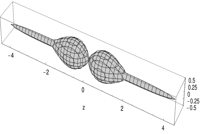
Figure 3: A boundary surface of $|\Xi_{n=1,\ell=0,0}(r,\theta,\phi)|^{2}$.

Now the solutions $\Xi_{n,\ell\neq 0,0}$ have nonzero total angular momentum while zero angular momentum in the $z$-direction, and the logarithm divergence for $\theta=0$ and $\pi$ is also present for all $\xi_{l,0}$, indicating that the $z$-axis plays a special role in the classical trajectories analogy. So it is possible to interpret that $\Xi_{n,\ell\neq 0,0}$ is related to two-dimensional motions taking place in planes containing the $z$-axis, i.e., to the 2D hydrogen atom. Figure 4 illustrates such interpretation for $\ell=2,m=0$. The 2D hydrogen atom has also been considered in the literature (see [30, 31, 32, 33, 34] and references therein), but its history is not as controversial as for the 1D case.

Finally, a word about $\Xi_{n,\ell,m\neq 0}$; since they do not belong to the Hilbert space, based on the above discussion and proceeding heuristically, it is tempting to interpret such solutions as the “contribution” due to the classical trajectories which come into collision with the nucleus, and the mathematical apparatus prudently avoids them explicitly (maybe a mathematical consequence of the uncertainty principle).

Figure 4: $|\xi_{2,0}(\theta)|$ and $|\Theta_{2,0}(\theta)|$ (dashed) as function of $\theta$.

4 Conclusions

One is naturally inclined to presume that higher dimensional quantum models carry somehow lower dimensional dynamics, and the study of such simpler models could mimics important aspects of the original one. Of course, in general the difficulties of performing such dimensional reductions are enormous, and usually carried out by “brute force.”

The case of the 3D hydrogen atom discussed in this work has revealed a particular and interesting framework: there are experimental evidence for the 1D hydrogen atom; the 3D hermitian model has just one self-adjoint extension, and its 3D eigenvalue equation presents formal solutions $\Xi_{n,\ell,0}$ that do not belong to the domain of the corresponding Hamiltonian operator; in spite of being formal eigenvectors, these solutions live in the underlying Hilbert space and present a component in the continuous subspace of the Hamiltonian so that, for an electron in such state, ionization can take place; these solutions have formally zero azimuthal angular momentum, with integrable probability densities, and are concentrated around the $z$-axis, indicating their 1D and 2D character for $\Xi_{n,0,0}$ and $\Xi_{n,\ell\neq 0,0}$, respectively. Summing up, such solutions are reminiscent of 1D and 2D classical trajectories and give a connection between the hydrogen atom in different dimensions.

How general is this framework? This is a fascinating open question, whose answer could eventually improve the interpretations.

In addition, notice that there is an attractive relation between the dimensional interpretations advocated in this work and the mathematical formalism, which exhausts the possibilities for (pseudo-)eigenvectors. For genuine 3D motion it presents eigenfunctions in the Hamiltonian operator domain; for 1D and 2D reminiscent trajectories it presents eigenfunctions in the Hilbert space but not in the domain of the operator; and for those colliding trajectories (axial divergence) the formal eigenfunctions do not belong to the Hilbert space.

Acknowledgments

AL-C thanks FAPESP. CRdeO thanks the partial support by CNPq.

References

- [1] Blank J, Exner P and Havlíček M 1994 Hilbert Space Operators in Quantum Physics (New York: AIP Press)
- [2] Reed M and Simon B 1972 Functional Analysis (New York: Academic Press); 1975 Fourier Analysis, Self-Adjointness (New York: Academic Press)
- [3] Thirring W 1981 Quantum Mechanics of Atoms and Molecules (New York: Springer)
- [4] Albeverio S, Gesztesy F, Hegh-Krohn R and Holden H 2005 Solvable models in quantum mechanics 2nd ed. (Providence: AMS Chelsea Publishing)
- [5] Fischer W, Leschke H and Müller P 1995 J. Math. Phys. 36 2313
- [6] Gesztesy F 1980 J. Phys. A: Math. Gen. 13 867
- [7] Cycon H L, Froese R G, Kirsch W and Simon B 1987 Schrödinger Operators (Berlin: Springer)
- [8] de Oliveira C R and do Carmo M C 1998 Rep. Math. Phys. 41 145
- [9] Arfken G B and Weber H J 2001 Mathematical Methods for Physicists 5th ed. (New York: Harcourt-Academic Press)
- [10] Wolfran Research: http://functions.wolfram.com/HypergeometricFunctions/
- [11] Pauling L and Wilson Jr E B 1963 Introduction to Quantum Mechanics with applications to Chemistry (New York: Dover) pp. 25-150
- [12] Loudon R 1959 Amer. J. Phys. 27 649
- [13] Andrews M 1966 Amer. J. Phys. 34 1194
- [14] Haines L K and Roberts D H 1969 Amer. J. Phys. 37 1145
- [15] Andrews M 1976 Amer. J. Phys. 44 1064
- [16] Gomes J F and Zimerman A H 1980 Amer. J. Phys. 48 579
- [17] Spector H N and Lee J 1985 Amer. J. Phys. 53 248
- [18] Davtyan L S, Pogosyan G S, Sissakian A N and Ter-Antonyan V M 1987 J. Phys. A: Math. Gen. 20 2765
- [19] Boya L J, Kmiecik M and Bohm A 1988 Phys. Rev. A 37 3567
- [20] Núñes-Yépez H N, Vargas C A and Salas-Brito A L 1989 Phys. Rev. A 39 4306
- [21] Liu W-C and Clark C W 1992 J. Phys. B: At. Mol. Opt. Phys. 25 L517
- [22] Oseguera U and de Llano M 1993 J. Math. Phys. 34 4575
- [23] Xianxi D, Dai J and Dai J 2001 Phys. Rev. A 55 2617
- [24] Li Q-S and Lu J 2001 Chem. Phys. Lett. 336 118
- [25] Jensen R V, Susskind S M and Sanders M M 1991 Phys. Rep. 201 1
- [26] Delone N B, Krainov B P and Shepelyansky D L 1983 Sov. Phys. Usp. 26 551
- [27] López-Castillo A and de Oliveira C R 2003 Chaos Sol. Fract. 15 859
- [28] Cole M W and Cohen M H 1969 Phys. Rev. Lett. 23 1238
- [29] Wong C M, McNeill J D, Gaffney K J, Ge N-H, Miller A D, Liu S H and Harris C B 1999 J. Phys. Chem. B 103 282
- [30] Yang X L, Guo S H, Chan F T, Wong K W and Ching W Y 1991 Phys. Rev. A 43 1186
- [31] del Castillo G F T and Villanueva A L 2001 Rev. Mex. Fis. 47 123
- [32] Robnik M and Romanovski V G 2003 J. Phys. A: Math. Gen. 36 7923
- [33] Villalba V M and Pino R 2003 Mod. Phys. Lett. B 17 1331
- [34] Parfitt D G W and Portnoi M E 2002 J. Math. Phys. 43 4681