Quantum Energy Inequalities and local covariance I: Globally hyperbolic spacetimes

Abstract

We begin a systematic study of Quantum Energy Inequalities (QEIs) in relation to local covariance. We define notions of locally covariant QEIs of both ‘absolute’ and ‘difference’ types and show that existing QEIs satisfy these conditions. Local covariance permits us to place constraints on the renormalised stress-energy tensor in one spacetime using QEIs derived in another, in subregions where the two spacetimes are isometric. This is of particular utility where one of the two spacetimes exhibits a high degree of symmetry and the QEIs are available in simple closed form. Various general applications are presented, including a priori constraints (depending only on geometric quantities) on the ground-state energy density in a static spacetime containing locally Minkowskian regions. In addition, we present a number of concrete calculations in both two and four dimensions which demonstrate the consistency of our bounds with various known ground- and thermal state energy densities. Examples considered include the Rindler and Misner spacetimes, and spacetimes with toroidal spatial sections. In this paper we confine the discussion to globally hyperbolic spacetimes; subsequent papers will also discuss spacetimes with boundary and other related issues.

I Introduction

Over the past 30 years, much effort has been devoted to calculations of the renormalised stress-energy tensor in ground states of quantum fields on stationary background spacetimes. Many analogous calculations have been made in flat spacetime equipped with reflecting boundaries, in connection with the Casimir effect. However, it would be fair to say that only limited qualititative insight has been gained. For example, the energy density is sometimes positive, and sometimes negative and there is no known way of predicting the sign in any general situations without performing the full calculations  (see, however, Kenneth and Klich (2006) for a situation where the sign can be predicted). At least analytically, these calculations are restricted to cases exhibiting a high degree of symmetry. The aim of this paper, and a companion paper Fewster and Pfenning , is to point out that there are situations in which one may gain some qualitative insight into the possible magnitude of the stress-energy tensor based on simple geometric considerations.

The situation we study in this paper arises when a spacetime contains a subspacetime which is isometric to (a subspacetime of) another spacetime, which will usually have nontrivial symmetries. By using quantum energy inequalities (QEIs) together with the locality properties of quantum field theory, we are then able to use information about the second (symmetric) spacetime to yield information about the stress-energy tensor of states on the first spacetime (which need have no global symmetries) in the region where the isometry holds. We will work on globally hyperbolic spacetimes in this paper, deferring the issue of spacetimes with boundary to a companion paper Fewster and Pfenning . As well as setting out the theory behind the method, we will demonstrate it in several locally Minkowskian spacetimes. Marecki Marecki has also illustrated our approach, by considering the case of spacetimes locally isometric to portions of exterior Schwarzschild. Also begun here for the free massless scalar field is a similar discussion for conformally related regions of two-dimensional spacetimes. In a separate paper we will extend this to the generalised Maxwell field in higher dimensional manifolds related by conformal diffeomorphisms.

To be more specific, consider a globally hyperbolic spacetime ${\bm{N}}$, consisting of a manifold of dimension $d\geq 2$, a Lorentzian metric with signature $+-\cdots-$, and choices of orientation and time-orientation (which, together, are required to fulfill the demands of global hyperbolicity) . Suppose an open subset of ${\bm{N}}$, when equipped with the metric and (time-)orientation inherited from ${\bm{N}}$, is a globally hyperbolic spacetime ${\bm{N}}^{\prime}$ in its own right. If, moreover, any causal curve in ${\bm{N}}$ whose endpoints lie in ${\bm{N}}^{\prime}$ is contained completely in ${\bm{N}}^{\prime}$, then we will call ${\bm{N}}^{\prime}$ a causally embedded globally hyperbolic subspacetime (c.e.g.h.s.) of ${\bm{N}}$. Our main interest will be in the situation where a c.e.g.h.s. ${\bm{N}}^{\prime}$ of ${\bm{N}}$ is isometric to a c.e.g.h.s. ${\bm{M}}^{\prime}$ of a second globally hyperbolic spacetime ${\bm{M}}$, with the isometry also respecting the (time-)orientation. (We speak of a causal isometry in this case.) By the principle of locality, we expect that any experiment conducted within ${\bm{N}}^{\prime}$ should have the same results as the same experiment [i.e., its isometric image] conducted in ${\bm{M}}^{\prime}$. No observer in ${\bm{N}}^{\prime}$ should be able to discern, by such local experiments that she does not, in fact, inhabit ${\bm{M}}^{\prime}$; in particular, energy densities in ${\bm{N}}^{\prime}$ should be subject to the same QEIs as those in ${\bm{M}}^{\prime}$. We will demonstrate explicitly that these expectations are met by the QEIs we employ.

Figure 1: Illustration for Example 1: The curve $\gamma$ in ${\bm{N}}$ is enclosed in a causally embedded globally hyperbolic subspacetime ${\bm{N}}^{\prime}$ which is causally isometric to a causally embedded globally hyperbolic subspacetime ${\bm{M}}^{\prime}$ of four-dimensional Minkowski space ${\bm{M}}$ under $\psi:{\bm{M}}^{\prime}\to{\bm{N}}^{\prime}$.

Among our results are the following, which we state for the case of a Klein–Gordon field of mass $m\geq 0$ in four dimensions:

Example 1: Suppose a timelike geodesic segment $\gamma$ of proper duration $\tau_{0}$ in a globally hyperbolic spacetime ${\bm{N}}$ can be enclosed in a c.e.g.h.s. ${\bm{N}}^{\prime}$ which is causally isometric to a c.e.g.h.s. of four-dimensional Minkowski space as shown in Fig. 1. Then any state $\omega$ of the Klein–Gordon field (of mass $m\geq 0$) on ${\bm{N}}$ obeys

$$\sup_{\gamma}\langle T_{ab}u^{a}u^{b}\rangle_{\omega}\geq-\frac{C_{4}}{\tau_{0}^{4}}$$ (1)

where the constant $C_{4}=3.169858\ldots$ (if $m>0$, one may obtain even more rapid decay).

Example 2: Suppose a globally hyperbolic spacetime ${\bm{N}}$ is stationary with respect to a timelike Killing field $t^{a}$ and admits the smooth foliation into constant time surfaces ${\bm{N}}\cong{\mathbb{R}}\times\Sigma$. Suppose the metric takes the Minkowski form (w.r.t. some coordinates) on ${\mathbb{R}}\times\Sigma_{0}$ for some subset $\Sigma_{0}$ of $\Sigma$ with nonempty interior. (We may suppose that $\Sigma_{0}$ has been taken to be maximal.) For any $x$ in the interior of $\Sigma_{0}$, let $r(x)$ be the radius of the largest Euclidean $3$-ball which can be isometrically embedded in $\Sigma_{0}$, centred on $x$, as in Fig. 2. Then any stationary Hadamard state  $\omega_{{\bm{N}}}$ on ${\bm{N}}$ obeys the bound

$$\langle T_{ab}n^{a}n^{b}\rangle_{\omega_{\bm{N}}}(t,x)\geq-\frac{C_{4}}{(2r(x))^{4}}$$ (2)

for any $x\in\Sigma_{0}$, where $n^{a}$ is the unit vector along $t^{a}$.

Figure 2: Diagram showing open ball about the point $x$ in Example 2.

Example 3: Suppose $\gamma:{\mathbb{R}}\to{\bm{N}}$ is a uniformly accelerated trajectory (parametrised by proper time) with proper acceleration $\alpha$, and suppose $\gamma$ can be enclosed within a c.e.g.h.s. ${\bm{N}}^{\prime}$ of ${\bm{N}}$ which is causally isometric to a c.e.g.h.s. of four-dimensional Minkowski space. Then, for any Hadamard state $\omega$ on ${\bm{N}}$, and any smooth compactly supported real-valued $g$, with $\int_{-\infty}^{\infty}g(\tau)^{2}\,d\tau=1$,

$$\liminf_{\tau_{0}\to\infty}\frac{1}{\tau_{0}}\int_{\gamma}\langle T_{ab}u^{a}u^{b}\rangle_{\omega}g(\tau/\tau_{0})^{2}\,d\tau\geq-\frac{11\alpha^{4}}{480\pi^{2}}\,.$$ (3)

Note the remarkable fact that the right-hand side is precisely the expected energy density in the Rindler vacuum state along the trajectory with constant proper accleration $\alpha$. In particular, if the energy density in some state $\omega$ is constant along $\gamma$, it must exceed or equal that of the Rindler vacuum. We emphasize that our derivation does not involve the Rindler vacuum, but only the Minkowski vacuum state two-point function and the QEIs.

Variants of these results hold in other dimensions, and also for other linear field equations such as the Maxwell and Proca fields (which we will treat elsewhere).

To prepare for our main discussion, it will be useful to make a few general remarks about quantum energy inequalities (QEIs), also often called simply quantum inequalities (QIs). QEIs have been quite intensively developed over the past decade, following Ford’s much earlier insight Ford (1978) that quantum field theory might act to limit the magnitude and duration of negative energy densities and/or fluxes, thereby preventing macroscopic violations of the second law of thermodynamics (see Fewster and Verch (2003) for rigorous links between QEIs and thermodynamical stability). Detailed reviews of QEIs may be found in Pfenning (1998); Fewster (2003); Roman (2004).

QEIs take various forms, but we will distinguish two basic types: absolute QEIs and difference QEIs. An absolute QEI bound consists of a set ${\mathscr{F}}$ of sampling tensors, i.e., second rank contravariant tensor fields against which the renormalised stress-energy tensor will be averaged, a class ${\mathcal{S}}$ of states of the theory (which may be chosen to have nice properties) and a map ${\mathcal{Q}}:{\mathscr{F}}\to{\mathbb{R}}$ such that

$$\int\langle T_{ab}\rangle_{\omega}f^{ab}\,d{\rm vol}\geq-{\mathcal{Q}}({\sf f})>-\infty$$ (4)

for all states $\omega\in{\mathcal{S}}$ . Here $T_{ab}$ is the renormalised stress-energy tensor defined in a manner compatible with Wald’s axioms Wald (1994), and we have adopted the convention that the same tensor may be written ${\sf f}$ (without indices) or $f^{ab}$ (with). We will permit ${\mathscr{F}}$ to include tensors singularly supported on timelike curves or other submanifolds of spacetime, so, for example, we can treat worldline averages such as

$$\int_{\gamma}\langle T_{ab}\rangle_{\omega}f^{ab}\,d\tau=\int_{I}\langle T_{ab}(\gamma(\tau))\rangle_{\omega}u^{a}u^{b}g(\tau)^{2}\,d\tau$$ (5)

where $\gamma$ is a smooth timelike curve parametrised by an open interval $I$ of proper time $\tau$, with velocity $u^{a}$, and for $g\in C_{0}^{\infty}({I})$. [To be precise, ${\mathscr{F}}$ is required to be a set of compactly supported distributions on smooth rank two covariant test tensor fields.]

Absolute QEIs are known [with explicit formulae for ${\mathcal{Q}}$, and specific ${\mathscr{F}}$ and ${\mathcal{S}}$] for (a) the scalar field of mass $m\geq 0$ in $d$-dimensional Minkowski space Ford and Roman (1995, 1997); Fewster and Eveson (1998) (see also Ford (1991) for $d\geq 2$), (b) the massless scalar and Fermi fields in arbitrary two-dimensional globally hyperbolic spacetimes Flanagan (1997); Vollick (2000); Flanagan (2002); Fewster (2004), (c) general (interacting) conformal field theories in two-dimensional Minkowski space Fewster and Hollands (2005), (d) a variety of higher spin linear fields in two- and four-dimensional Minkowski space Ford and Roman (1997); Pfenning (2002); Fewster and Pfenning (2003); Fewster and Mistry (2003); Dawson (2006); Yu and Wu (2004); B. Hu and Zhang (2006). For the most part only worldline bounds involving averages of the form Eq. (5) have been studied; it has been found that replacing $g$ by a scaled version $\tau_{0}^{-1/2}g(\tau/\tau_{0})$ has the effect of sending the QEI bound to zero as $\tau_{0}^{-d}$ (or faster, for massive fields) as $\tau_{0}\to\infty$, where $d$ is the spacetime dimension.

Difference QEI bounds also involve the specification of ${\mathscr{F}}$ and ${\mathcal{S}}$ as before, but now the bound sought takes the form

$$\int\left[\langle T_{ab}\rangle_{\omega}-\langle T_{ab}\rangle_{\omega_{0}}\right]f^{ab}\,d{\rm vol}\geq-{\mathcal{Q}}({\sf f},\omega_{0})>-\infty\,,$$ (6)

where $\omega_{0}$ is called the reference state. If the theory were represented in a Fock space built on $\omega_{0}$ (when this is possible) the left-hand side would be an average of the normal ordered stress-energy tensor. However it is not always necessary to assume that $\omega$ and $\omega_{0}$ are represented in this way. Difference QEIs have proved to be the easiest to establish in curved spacetimes, or where boundaries are present. First developed in the case of (ultra)static spacetimes with the (ultra)static ground state chosen as the reference state $\omega_{0}$ Pfenning and Ford (1997, 1998); Fewster and Teo (1999); Pfenning (2002), they are now known for scalar, spin-$1/2$, and spin-$1$ fields in arbitrary globally hyperbolic spacetimes Fewster (2000); Fewster and Verch (2002); Fewster and Pfenning (2003). In these general results, ${\mathcal{S}}$ is the class of Hadamard states and the bounds are sufficiently general that $\omega_{0}$ may be any element of ${\mathcal{S}}$, so ${\mathcal{Q}}$ becomes a function ${\mathcal{Q}}:{\mathscr{F}}\times{\mathcal{S}}\to{\mathbb{R}}$. The general results do not make use of a Hilbert space representation.

Clearly, difference and absolute QEIs are quite closely related. In particular, Wald’s fourth axiom requires $\langle T_{ab}\rangle_{\omega_{0}}$ to vanish identically if $\omega_{0}$ is the Minkowski vacuum, so difference QEIs become absolute in this case. [The extension of this observation to locally Minkowskian spaces is a key idea in this paper.] More generally, we may convert a difference QEI to an absolute QEI by moving all the terms in $\omega_{0}$ onto the right-hand side. In cases where the renormalised stress-energy tensor is known explicitly for the reference state, this is perfectly satisfactory. However, there are two (related) drawbacks: (i) there is no canonical choice of reference state $\omega_{0}$ in a general spacetime (which might have no timelike Killing fields, for example); (ii) one does not normally have available a closed form expression for $\langle T_{ab}\rangle_{\omega_{0}}$ for any state on a general spacetime, so the QEI bound becomes somewhat inexplicit. This weakens the power of QEIs to constrain exotic spacetime configurations such as macroscopic traversable wormholes or ‘warp drive’. (On sufficiently small scales, one expects that the absolute QEI bounds should strongly resemble those of Minkowski space—as first argued in Ford and Roman (1996), and proven in various situations in Pfenning and Ford (1998) and Fewster (2004)—however one still needs to know the magnitude of $\langle T_{ab}\rangle_{\omega_{0}}$ to know on what scales this approximation holds.)

The present paper and its companion represent first steps towards absolute QEIs in more general spacetimes, starting with spacetimes containing regions isometric to others where reference states are known. Work is under way on generally applicable absolute QEIs and will be reported elsewhere; however we expect the results and methods presented here to be of continuing interest, as they reduce to very simple geometrical conditions.

The paper is structured as follows. In Sec. II we give a brief introduction to some of the relevant notions of locally covariant quantum field theory before defining locally covariant QEIs and developing their simple properties in Sec. II.3. The following two subsections show how existing QEIs in the literature may be expressed in the locally covariant framework, and address some technical points along the way. In Sec. III we show how local covariance permits a priori bounds to be placed on energy densities in spacetimes with Minkowskian subspacetimes using geometric data. The main technique here, in addition to local covariance, is the conversion of QEIs to eigenvalue problems, first introduced in Fewster and Teo (2000). These are applied in Sec. IV to specific spacetime models where the energy densities of ground- and thermal states are known, permitting comparison with our a priori bounds. In some cases these bounds are saturated by the exact values. After a summary, the appendices collect various results needed in the main text.

II Quantum energy inequalities and local covariance

II.1 Geometrical preliminaries

Suppose two globally hyperbolic spacetimes of the same dimension, ${\bm{M}}_{1}$ and ${\bm{M}}_{2}$, are given (we denote the corresponding manifolds and metrics by $M_{i}$, ${\bm{g}}_{i}$ for $i=1,2$). An isometric embedding of ${\bm{M}}_{1}$ in ${\bm{M}}_{2}$ is a smooth map $\psi:M_{1}\to M_{2}$ which is a diffeomorphism of $M_{1}$ onto its range $\psi(M_{1})$ in $M_{2}$ and so that the pull-back $\psi^{*}{\bm{g}}_{2}$ is everywhere equal to ${\bm{g}}_{1}$ on $M_{1}$. In local coordinates,

$$g_{1\,ab}(x)=\frac{\partial y^{a^{\prime}}}{\partial{x}^{a}}\frac{\partial y^{b^{\prime}}}{\partial{x}^{b}}g_{2\,a^{\prime}b^{\prime}}(y)$$ (7)

should hold for all $x\in M_{1}$, where $y=\psi(x)$. We do require that all of $M_{1}$ is mapped into $M_{2}$, but we do not require that the image of $M_{1}$ under $\psi$ consists of the whole of $M_{2}$. There are two possible choices of orientation and time orientation on $\psi(M_{1})$: that induced by $\psi$ from the (time-)orientation of ${\bm{M}}_{1}$, and that inherited from ${\bm{M}}_{2}$. If these coincide and we have the further property that every causal curve in ${\bm{M}}_{2}$ with endpoints in $\psi(M_{1})$ lies entirely in $\psi(M_{1})$, then we say that $\psi$ is a causal isometric embedding. An important class of examples arises where ${\bm{M}}_{1}$ is a causally embedded globally hyperbolic subspacetime (c.e.g.h.s.) of ${\bm{M}}_{2}$ as defined in Sec. I, in which case $\psi$ is simply the identity map. It is also worth mentioning an example of a non-causal embedding, namely, the ‘helical strip’ described by Kay Kay (1992). In this example a long thin diamond region of two dimensional Minkowski space is isometrically embedded in a ‘timelike cylinder’ which is the quotient of Minkowski space by a spacelike translation. The wrapping is arranged so that points which are spacelike separated in the original diamond are timelike separated in the geometry of the timelike cylinder. The definition of a causal embedding is designed precisely to ensure that the induced and inherited causal structures cannot differ in this way.

II.2 Local covariance

The relevance of local covariance to quantum field theory on manifolds has long been understood Kay (1979); Dimock (1980) but has recently been put in a new setting by Brunetti, Fredenhagen and Verch Brunetti et al. (2003) (see also Verch (2001) and R. Brunetti and Ruzzi (2006)) and related work of Hollands and Wald (see, e.g., Hollands and Wald (2001, 2002)). This provides a very elegant and general framework for local covariance in the language of category theory. However, we will only need a few of the main ideas of this analysis and will not describe the whole structure.

In this section, we will restrict ourselves to the Klein–Gordon field of mass $m\geq 0$, although similar comments can be made for the Dirac, Maxwell, and Proca fields. There is a well-defined quantisation of the theory on any globally hyperbolic spacetime ${\bm{M}}$, in terms of an algebra of observables ${\mathfrak{A}}_{\bm{M}}$ and a space of Hadamard states ${\mathcal{S}}_{\bm{M}}$ which determine expectation values for observables in ${\mathfrak{A}}_{\bm{M}}$. For the purposes of this section, it suffices to know that ${\mathfrak{A}}_{\bm{M}}$ is generated by smeared field objects $\Phi_{\bm{M}}(f)$ labelled by smooth, compactly supported test functions $f\in C_{0}^{\infty}({{\bm{M}}})$, subject to relations expressing the field equation and commutation relations, and the hermiticity of the field. (The structure is given in detail in Appendix A.) The Hadamard states of the theory are those states on ${\mathfrak{A}}_{\bm{M}}$ whose two-point functions have singularities of the Hadamard form, which at leading order are just those of the Minkowski vacuum two-point function. More precisely Kay and Wald (1991), on any causal normal neighbourhood ${\cal O}$ in ${\bm{M}}$ there is a sequence of bidistributions $H_{n}$ so that (for any $n$) the two-point function of any Hadamard state differs from $H_{n}$ on ${\cal O}$ by a state-dependent function of class $C^{n}$. It is of key importance that $H_{n}(x,x^{\prime})$ is fixed entirely by the local metric and causal structure, through the Hadamard recursion relations. Given a Hadamard state $\omega$, we may construct the expected renormalised stress-energy tensor $\langle T_{ab}\rangle_{\omega}$ by the point-splitting technique (see, e.g., Wald (1994)): first subtract $H_{n}$ from the two-point function (for $n\geq 2$), then apply appropriate derivatives before taking the points together again. Next, one subtracts a term of the form $Qg_{ab}$, where $Q$ is locally determined (and state-independent), in order to ensure that the resulting tensor is conserved and vanishes in the Minkowski vacuum state. The tensor defined in this way obeys Wald’s axioms mentioned above; however, these axioms would also be satisfied if one were to add a conserved local curvature term. Such terms are sometimes described as undetermined or arbitrary; we take the view, however, that they are part of the specification of the theory, just as the mass and conformal coupling are, even though they do not appear explicitly in the Lagrangian (a similar attitude is expressed in Flanagan and Wald (1996)). For simplicity, and because our main applications will concern locally Minkowskian spacetimes, we will assume that these terms are absent – that is, we restrict to those scalar particle species for which this is the case.

The above structure is locally covariant in the following sense. Suppose a globally hyperbolic spacetime ${\bm{M}}$ is embedded in a globally hyperbolic spacetimes ${\bm{N}}$ by a causal isometry $\psi$, and let $\psi_{*}$ denote the push-forward map on test functions. That is, $\psi_{*}:C_{0}^{\infty}({{\bm{M}}})\to C_{0}^{\infty}({{\bm{N}}})$ is defined by

$$(\psi_{*}f)(y)=\left\{\begin{array}[]{cl}f(\psi^{-1}(y))&\hbox{if $y=\psi(x)$ for some $x\in{\bm{M}}$}\\ 0&\hbox{otherwise.}\end{array}\right.$$ (8)

Then there is a natural mapping of the field on ${\bm{M}}$ to the field on ${\bm{N}}$ given by $\Phi_{\bm{M}}(f)\mapsto\Phi_{\bm{N}}(\psi_{*}f)$; we also write this as $\psi_{*}(\Phi_{\bm{M}}(f))=\Phi_{\bm{N}}(\psi_{*}f)$. Moreover, $\psi_{*}$ can be extended to any element of ${\mathfrak{A}}_{\bm{M}}$, respecting the algebraic relations and mapping the identity in ${\mathfrak{A}}_{\bm{M}}$ to the identity in ${\mathfrak{A}}_{\bm{N}}$; technically, it is a unit-preserving injective $*$-homomorphism of ${\mathfrak{A}}_{\bm{M}}$ into ${\mathfrak{A}}_{\bm{N}}$.

On account of the correspondence $\Phi_{\bm{M}}(f)\mapsto\Phi_{\bm{N}}(\psi_{*}f)$, we say that the field is covariant [the transformation goes ‘in the same direction’ as $\psi$; see the remarks below on the underlying category theory at the end of Appendix A]. By contrast, the state spaces transform in a contravariant way [in the ‘opposite direction’ to $\psi$]: for any state $\omega$ on ${\mathfrak{A}}_{\bm{N}}$ there is a pulled-back state, which we denote $\psi^{*}\omega$, on ${\mathfrak{A}}_{\bm{M}}$, so that the expectation values of $A\in{\mathfrak{A}}_{\bm{M}}$ and $\psi_{*}A\in{\mathfrak{A}}_{\bm{N}}$ are related by

$$\langle A\rangle_{\psi^{*}\omega}=\langle\psi_{*}A\rangle_{\omega}\,.$$ (9)

The use of pull-back notation may be justified by the observation that Eq. (9) entails that the $n$-point functions of the two states are related by

$$\langle\Phi_{\bm{M}}(x_{1})\cdots\Phi_{\bm{M}}(x_{n})\rangle_{\psi^{*}\omega}=\langle\Phi_{\bm{N}}(\psi(x_{1}))\cdots\Phi_{\bm{N}}(\psi(x_{n}))\rangle_{\omega}$$ (10)

(adopting an ‘unsmeared’ notation). That is, the $n$-point function of $\psi^{*}\omega$ is simply the pull-back of the $n$-point function of $\omega$ by $\psi$ (or more precisely, by the duplication of $\psi$ across $n$ copies of ${\bm{M}}$). This has an important consequence when the state $\omega$ is Hadamard, i.e., $\omega\in{\mathcal{S}}_{\bm{N}}$: because the Hadamard condition is based on the local metric and causal structure, both of which are preserved by $\psi$, it is clear that $\psi^{*}\omega$ is also Hadamard. (A more elegant proof of this Brunetti et al. (2003) is to use Radzikowski’s characterisation of the Hadamard condition in terms of the wave-front set of the two-point function Radzikowski (1996), and the transformation properties of the wave-front set under pull-backs.) This may be expressed by the inclusion $\psi^{*}{\mathcal{S}}_{\bm{N}}\subset{\mathcal{S}}_{\bm{M}}$.

As noted above, the expectation values of the stress-energy tensor is also constructed in a purely local fashion from the two-point function of the state. It therefore follows that

$$\langle T_{{\bm{M}}\,ab}(x)\rangle_{\psi^{*}\omega}=\frac{\partial y^{a^{\prime}}}{\partial x^{a}}\frac{\partial y^{b^{\prime}}}{\partial x^{b}}\langle T_{{\bm{N}}\,a^{\prime}b^{\prime}}(y)\rangle_{\omega}$$ (11)

where we have written $y=\psi(x)$: like the $n$-point functions, the expected stress-energy tensor in state $\psi^{*}\omega$ is simply the pull-back of that in state $\omega$. In coordinate-free notation we may write

$$\langle{\sf T}_{\bm{M}}\rangle_{\psi^{*}\omega}=\psi^{*}\langle{\sf T}_{\bm{N}}\rangle_{\omega}\,.$$ (12)

In the above equations we have written the stress-energy tensor as if it is an element of the algebra ${\mathfrak{A}}_{\bm{M}}$, which it is not. One may proceed in two ways: either interpreting Eq. (12) as the extension of Eq. (9) to an algebra of Wick polynomials which contains ${\mathfrak{A}}_{\bm{M}}$ as a subalgebra, and in which ${\sf T}_{{\bm{M}}}$ may be defined as a locally covariant field Hollands and Ruan (2002); Hollands and Wald (2001). For our purposes, however, it will be simpler to define the smeared stress-energy tensor only through its expectation values; more technically, we think of it as a linear functional on the space of Hadamard states, with the notation $\langle{\sf T}_{\bm{M}}({\sf f})\rangle_{\omega}$ expressing the value of this functional applied to the state $\omega$. This has the advantage that one may deal with all Hadamard states, rather than those which extend to the Wick algebra Hollands and Ruan (2002).

We emphasise the fact that states are pulled back in this setting; although one could push forward a state $\omega\in{\mathcal{S}}_{\bm{M}}$ to obtain a state on ${\mathfrak{A}}_{\psi({\bm{M}})}$, there is no guarantee that this can be extended to a Hadamard state on ${\mathfrak{A}}_{\bm{N}}$, and indeed, such extensions do not always exist. For example, the Rindler vacuum state on the Rindler wedge is Hadamard in the interior of the wedge Sahlmann and Verch (2000), but cannot be extended to a Hadamard state on the whole of Minkowski because its stress-energy tensor diverges at the boundary of the wedge. See Fewster et al. for further discussion of these issues.

Figure 3: If ${\bm{M}}$ is embedded in ${\bm{N}}$ by a causal isometry $\psi$, then test functions and smeared fields may be pushed forwards from ${\bm{M}}$ to ${\bm{N}}$, while states (and expectation values) are pulled back from ${\bm{N}}$ to ${\bm{M}}$.

II.3 QEIs in a locally covariant setting

We now introduce two types of locally covariant QEIs. A more abstract (and general) definition can be given in the language of categories—this will be pursued elsewhere. Recall that a set of sampling tensors on a globally hyperbolic spacetime is a set of compactly supported distributions on smooth second rank covariant tensor fields.

Definition II.1

A locally covariant absolute QEI assigns to each globally hyperbolic spacetime ${\bm{M}}$ a set of sampling tensors ${\mathscr{F}}_{\bm{M}}$ on ${\bm{M}}$ and a map ${\mathcal{Q}}_{\bm{M}}:{\mathscr{F}}_{\bm{M}}\to{\mathbb{R}}$ such that (i) we have

$$\langle{\sf T}_{\bm{M}}({\sf f})\rangle_{\omega}\geq-{\mathcal{Q}}_{\bm{M}}({\sf f})$$ (13)

for all ${\sf f}\in{\mathscr{F}}_{\bm{M}}$ and $\omega\in{\mathcal{S}}_{\bm{M}}$, and (ii) if $\psi:{\bm{M}}\to{\bm{N}}$ is a causal isometric embedding then $\psi_{*}{\mathscr{F}}_{\bm{M}}\subset{\mathscr{F}}_{\bm{N}}$ and

$${\mathcal{Q}}_{\bm{M}}({\sf f})={\mathcal{Q}}_{\bm{N}}(\psi_{*}{\sf f})$$ (14)

for all ${\sf f}\in{\mathscr{F}}_{\bm{M}}$. (We might also express this in the form ${\mathcal{Q}}_{\bm{M}}=\psi^{*}{\mathcal{Q}}_{\bm{N}}$.)

A locally covariant difference QEI assigns to each globally hyperbolic ${\bm{M}}$ a set of sampling tensors ${\mathscr{F}}_{\bm{M}}$ as before, and a map ${\mathcal{Q}}_{\bm{M}}:{\mathscr{F}}_{\bm{M}}\times{\mathcal{S}}_{\bm{M}}\to{\mathbb{R}}$ such that (i)

$$\langle{\sf T}_{\bm{M}}({\sf f})\rangle_{\omega}-\langle{\sf T}_{\bm{M}}({\sf f})\rangle_{\omega_{0}}\geq-{\mathcal{Q}}_{\bm{M}}({\sf f},\omega_{0})$$ (15)

for each ${\sf f}\in{\mathscr{F}}_{\bm{M}}$ and all $\omega,\omega_{0}\in{\mathcal{S}}_{\bm{M}}$; (ii)

$${\mathcal{Q}}_{\bm{M}}({\sf f},\psi^{*}\omega_{0})={\mathcal{Q}}_{\bm{N}}(\psi_{*}{\sf f},\omega_{0})$$ (16)

holds for all ${\sf f}\in{\mathscr{F}}_{\bm{M}}$ and $\omega_{0}\in{\mathcal{S}}_{\bm{N}}$.

We will shortly give examples of each type: Flanagan’s two-dimensional QEIs for massless fields Flanagan (2002) will be exhibited as a locally covariant absolute QEI, while (generalisations of) the QEI obtained in Fewster (2000) provide examples of locally covariant difference QEIs. Before that, let us examine some simple consequences of these definitions.

First, suppose that ${\bm{M}}^{\prime}$ is a c.e.g.h.s. of ${\bm{M}}$, so the identity map $\imath:{\bm{M}}^{\prime}\to{\bm{M}}$ is a causal isometric embedding, and we must have $\imath_{*}{\mathscr{F}}_{{\bm{M}}^{\prime}}\subset{\mathscr{F}}_{\bm{M}}$ and ${\mathcal{Q}}_{{\bm{M}}^{\prime}}({\sf f})={\mathcal{Q}}_{{\bm{M}}}(\imath_{*}{\sf f})$. It is sensible to drop the identity mappings, and write the above in the form

$${\mathscr{F}}_{{\bm{M}}^{\prime}}\subset{\mathscr{F}}_{\bm{M}}\,,\quad{\rm and}\quad{\mathcal{Q}}_{{\bm{M}}^{\prime}}({\sf f})={\mathcal{Q}}_{{\bm{M}}}({\sf f})~{}\hbox{for all ${\sf f}\in{\mathscr{F}}_{{\bm{M}}^{\prime}}$.}$$ (17)

If $\psi:{\bm{M}}^{\prime}\to{\bm{N}}$ is a causal isometric embedding we then obtain

$${\mathcal{Q}}_{{\bm{M}}}({\sf f})={\mathcal{Q}}_{{\bm{M}}^{\prime}}({\sf f})={\mathcal{Q}}_{{\bm{N}}}(\psi_{*}{\sf f})$$ (18)

for all ${\sf f}\in{\mathscr{F}}_{{\bm{M}}^{\prime}}$. As one would expect, this shows that locally covariant absolute QEIs are indifferent to the larger spacetime; one obtains the same bound whether one is in ${\bm{M}}^{\prime}$ or its image ${\bm{N}}^{\prime}$ in ${\bm{N}}$. Although this barely extends the original definition, it is worth isolating it as a separate result.

Proposition II.2

Suppose a c.e.g.h.s. ${\bm{M}}^{\prime}$ of ${\bm{M}}$ is causally isometric to a c.e.g.h.s. ${\bm{N}}^{\prime}$ of ${\bm{N}}$ under the map $\psi$. Then a locally covariant absolute QEI obeys

$${\mathcal{Q}}_{\bm{M}}({\sf f})={\mathcal{Q}}_{\bm{N}}(\psi_{*}{\sf f})$$ (19)

for all ${\sf f}\in{\mathscr{F}}_{{\bm{M}}^{\prime}}\subset{\mathscr{F}}_{\bm{M}}$.

Figure 4: Diagram showing the various spacetimes and embeddings in Sec. II.3

Let us now examine locally covariant difference QEIs in this situation. Given arbitrary Hadamard states $\omega_{\bm{M}}\in{\mathcal{S}}_{\bm{M}}$ and $\omega_{\bm{N}}\in{\mathcal{S}}_{\bm{N}}$ on the parent spacetimes ${\bm{M}}$ and ${\bm{N}}$, there are states $\imath^{*}\omega_{\bm{M}}$ and $\psi^{*}\omega_{\bm{N}}$ in ${\mathcal{S}}_{{\bm{M}}^{\prime}}$, i.e., Hadamard states on ${\mathfrak{A}}_{{\bm{M}}^{\prime}}$. Applying the difference QEI to $\psi^{*}\omega_{\bm{N}}$ with $\imath^{*}\omega_{\bm{M}}$ as reference state, we find

$$\langle{\sf T}_{{\bm{M}}^{\prime}}({\sf f})\rangle_{\psi^{*}\omega_{\bm{N}}}-\langle{\sf T}_{{\bm{M}}^{\prime}}({\sf f})\rangle_{\imath^{*}\omega_{\bm{M}}}\geq-{\mathcal{Q}}_{{\bm{M}}^{\prime}}({\sf f},\imath^{*}\omega_{\bm{M}})=-{\mathcal{Q}}_{{\bm{M}}}(\imath_{*}{\sf f},\omega_{\bm{M}})$$ (20)

where we have used the transformation property Eq. (16). On the other hand, we could equally well apply the difference QEI to $\imath^{*}\omega_{\bm{M}}$, with $\psi^{*}\omega_{\bm{N}}$ as reference state, to obtain

$$\langle{\sf T}_{{\bm{M}}^{\prime}}({\sf f})\rangle_{\imath^{*}\omega_{\bm{M}}}-\langle{\sf T}_{{\bm{M}}^{\prime}}({\sf f})\rangle_{\psi^{*}\omega_{\bm{N}}}\geq-{\mathcal{Q}}_{{\bm{M}}^{\prime}}({\sf f},\psi^{*}\omega_{\bm{N}})=-{\mathcal{Q}}_{{\bm{N}}}(\psi_{*}{\sf f},\omega_{\bm{N}})$$ (21)

Combining these inequalities yields

$${\mathcal{Q}}_{{\bm{N}}}(\psi_{*}{\sf f},\omega_{\bm{N}})\geq\langle{\sf T}_{{\bm{M}}^{\prime}}({\sf f})\rangle_{\psi^{*}\omega_{\bm{N}}}-\langle{\sf T}_{{\bm{M}}^{\prime}}({\sf f})\rangle_{\imath^{*}\omega_{\bm{M}}}\geq-{\mathcal{Q}}_{{\bm{M}}}(\imath_{*}{\sf f},\omega_{\bm{M}})\,;$$ (22)

we may also use the covariance of ${\sf T}$ to reexpress the central member of this inequality in terms of expectation values on ${\bm{N}}$ and ${\bm{M}}$, rather than ${\bm{M}}^{\prime}$. The result, on dropping identity mappings from the notation, is the following.

Proposition II.3

Suppose a c.e.g.h.s. ${\bm{M}}^{\prime}$ of ${\bm{M}}$ is causally isometric to a c.e.g.h.s. ${\bm{N}}^{\prime}$ of ${\bm{N}}$ under the map $\psi$. Then a locally covariant difference QEI obeys

$${\mathcal{Q}}_{{\bm{N}}}(\psi_{*}{\sf f},\omega_{\bm{N}})\geq\langle{\sf T}_{{\bm{N}}}(\psi_{*}{\sf f})\rangle_{\omega_{\bm{N}}}-\langle{\sf T}_{{\bm{M}}}({\sf f})\rangle_{\omega_{\bm{M}}}\geq-{\mathcal{Q}}_{{\bm{M}}}({\sf f},\omega_{\bm{M}})\,,$$ (23)

for all ${\sf f}\in{\mathscr{F}}_{{\bm{M}}^{\prime}}\subset{\mathscr{F}}_{\bm{M}}$ and any $\omega_{\bm{M}}\in{\mathcal{S}}_{\bm{M}}$, $\omega_{\bm{N}}\in{\mathcal{S}}_{\bm{N}}$.

Note that the QEIs used are those associated with the full spacetimes ${\bm{M}}$ and ${\bm{N}}$; similarly, the states $\omega_{\bm{M}}$, $\omega_{\bm{N}}$ are states of the field on the full spacetimes. However, the isometry $\psi$ connects only portions of the spacetime together and the restriction on the support of ${\sf f}$ is therefore crucial: in general the above result will not hold when sampling extends outside the isometric region. It is also worth noting that we have both lower and upper bounds.

In this paper, we will study the simplest possible setting for this result, in which ${\bm{M}}$ is Minkowski spacetime and $\omega_{\bm{M}}$ is the Minkowski vacuum state. However other situations are possible. For example, Marecki Marecki has employed our framework in the case where ${\bm{M}}$ is the exterior Schwarzschild spacetime and $\omega_{\bm{M}}$ is the Boulware vacuum. In the Minkowski case, the result simplifies because the renormalised stress-energy tensor vanishes in the state $\omega_{\bm{M}}$, and we have the following statement.

Corollary II.4

Suppose a c.e.g.h.s. ${\bm{M}}^{\prime}$ of Minkowski space ${\bm{M}}$ is causally isometric to a c.e.g.h.s. ${\bm{N}}^{\prime}$ of ${\bm{N}}$ under the map $\psi$. Then a locally covariant difference QEI obeys

$${\mathcal{Q}}_{{\bm{N}}}(\psi_{*}{\sf f},\omega_{\bm{N}})\geq\langle{\sf T}_{{\bm{N}}}(\psi_{*}{\sf f})\rangle_{\omega_{\bm{N}}}\geq-{\mathcal{Q}}_{{\bm{M}}}({\sf f},\omega_{\bm{M}})\,,$$ (24)

for all ${\sf f}\in{\mathscr{F}}_{{\bm{M}}^{\prime}}\subset{\mathscr{F}}_{\bm{M}}$ and any $\omega_{\bm{N}}\in{\mathcal{S}}_{\bm{N}}$, where $\omega_{\bm{M}}$ is the Minkowski vacuum state.

II.4 A locally covariant absolute QEI for massless fields in two dimensions

The QEI we now describe was originally developed by Flanagan Flanagan (1997) for the massless scalar field in two dimensional Minkowski space, in work which was subsequently generalised to curved spacetimes Vollick (2000); Flanagan (2002); Fewster (2004) and also to arbitrary unitary positive energy conformal field theories in two dimensional Minkowski space Fewster and Hollands (2005). The results of Flanagan (2002) were obtained for two-dimensional spacetimes globally conformal to the whole of Minkowski space; as noted in Fewster (2004), however, any point of a globally hyperbolic two-dimensional spacetime has a (causally embedded) neighbourhood which is conformal to the whole of Minkowski space, and to which Flanagan’s result applies.

We first state the result of Flanagan (2002), and then show that it meets our definition of a locally covariant absolute QEI. Let ${\bm{M}}$ be a globally hyperbolic two-dimensional spacetime, and suppose that $\gamma$ is a smooth, future-directed timelike curve, parametrised by proper time $\tau\in I$, which is completely contained within a c.e.g.h.s. ${\bm{M}}^{\prime}$ of ${\bm{M}}$, such that ${\bm{M}}^{\prime}$ is globally conformal to the whole of two-dimensional Minkowski space. Then all Hadamard states $\omega$ on ${\bm{M}}$ obey the QEI

$$\int_{I}\langle T_{{\bm{M}}\,ab}u^{a}u^{b}\rangle_{\omega}(\gamma(\tau))g(\tau)^{2}\,d\tau\geq-\frac{1}{6\pi}\int_{I}\left[g^{\prime}(\tau)^{2}+g(\tau)^{2}\left\{R_{{\bm{M}}}(\gamma(\tau))-a^{c}(\tau)a_{c}(\tau)\right\}\right]\,d\tau$$ (25)

for any smooth, real-valued $g$ compactly supported in $I$ , where $u^{a}$ is the two-velocity of $\gamma$, $a^{c}$ is its acceleration and $R_{\bm{M}}$ is the scalar curvature on ${\bm{M}}$. [Note that Flanagan (2002) uses conventions in which $u^{a}u_{a}<0$ for timelike $u^{a}$; the bound is therefore modified slightly.]

As we now describe, Flanagan’s bound is a locally covariant absolute QEI. Given $I$, $\gamma$ and $g$ as above, we may define a compactly supported distribution ${\sf f}_{I,\gamma,g}$ acting on smooth second rank covariant tensor fields ${\sf t}$, by

$${\sf f}_{I,\gamma,g}({\sf t})=\int_{I}g(\tau)^{2}u^{a}u^{b}t_{ab}|_{\gamma(\tau)}\,d\tau\,.$$ (26)

Our set of sampling tensors ${\mathscr{F}}^{\rm conf}_{\bm{M}}$ (‘conf’ abbreviating ‘conformal’) will be the set of all distributions formed in this way. [A distribution of the form ${\sf f}_{I,\gamma,g}$ is singularly supported on the curve $\gamma$; we could also write it in the form

$$f_{I,\gamma,g}^{ab}|_{p}=\int_{I}u^{a}u^{b}g(\tau)^{2}\delta_{\gamma(\tau)}(p)\,d\tau$$ (27)

where $\delta_{q}(p)$ is the $\delta$-function at $q$, obeying $\int_{\bm{M}}\delta_{q}(p)F(p)d{\rm vol}=F(q)$.]

The QEI bound ${\mathcal{Q}}^{\rm conf}_{\bm{M}}$ is then defined by

$${\mathcal{Q}}^{\rm conf}_{\bm{M}}({\sf f})=\frac{1}{6\pi}\int_{I}\left[g^{\prime}(\tau)^{2}+g(\tau)^{2}\left\{R_{{\bm{M}}}(\gamma(\tau))-a^{c}(\tau)a_{c}(\tau)\right\}\right]\,d\tau\$$ (28)

for any $I$, $\gamma$, $g$ for which ${\sf f}={\sf f}_{I,\gamma,g}$. For this to make sense, we must ensure that the right-hand side is unchanged if we replace $I$, $\gamma$ and $g$ by $\widetilde{I}$, $\widetilde{\gamma}$ and $\widetilde{g}$ such that ${\sf f}_{I,\gamma,g}={\sf f}_{\widetilde{I},\widetilde{\gamma},\widetilde{g}}$. Since $\gamma$ and $\gamma^{\prime}$ are both assumed to be parametrised by proper time, our two sampling tensors must be related in a simple way: ${\rm supp}\,\widetilde{g}$ is the translation of ${\rm supp}\,g$ by some $\tau_{0}$, so that $\widetilde{\gamma}(\tau)=\gamma(\tau+\tau_{0})$, $\widetilde{g}(\tau)^{2}=g(\tau+\tau_{0})^{2}$ for all $\tau\in{\rm supp}\,\widetilde{g}$. The only possible ambiguity stems from the fact that $\widetilde{g}(\tau)$ and $g(\tau+\tau_{0})$ mught differ by a relative sign which can change at zeros of $\widetilde{g}$ of infinite order. However, it is simple to show that, nevertheless, $\widetilde{g}^{\prime}(\tau)^{2}=g^{\prime}(\tau+\tau_{0})^{2}$ , ensuring that the right-hand side of Eq. (28) is unchanged under the reparametrization of ${\sf f}$.

The bound Eq. (25) now takes the form of Eq. (13), so it remains only to verify that ${\mathscr{F}}^{\rm conf}_{\bm{M}}$ and ${\mathcal{Q}}^{\rm conf}_{\bm{M}}$ have the required transformation properties. Suppose $\psi:{\bm{M}}\to{\bm{N}}$ is a causal isometric embedding. The push-forward $\psi_{*}$ acts on ${\sf f}_{I,\gamma,g}\in{\mathscr{F}}^{\rm conf}_{\bm{M}}$ so that, for any smooth tensor field $t_{ab}$ on ${\bm{N}}$, we have

$$(\psi_{*}{\sf f}_{I,\gamma,g})({\sf t}) = {\sf f}_{I,\gamma,g}(\psi^{*}{\sf t})$$ (29)

$$= \int_{I}g(\tau)^{2}u^{a}u^{b}(\psi^{*}{\sf t})_{ab}|_{\gamma(\tau)}\,d\tau$$

$$= \int_{I}g(\tau)^{2}(\psi^{*}{\sf u})^{a}(\psi^{*}{\sf u})^{b}t_{ab}|_{\gamma(\tau)}\,d\tau$$

$$= {\sf f}_{I,\psi\circ\gamma,g}({\sf t})\,.$$

Now the image curve $\psi\circ\gamma$ can certainly be enclosed in a c.e.g.h.s. of ${\bm{N}}$ which is conformal to the whole of Minkowski space: namely the image under $\psi$ of that which enclosed $\gamma$. Moreover, the image curve has velocity $\psi^{*}{\sf u}$. It is therefore clear that $\psi_{*}{\sf f}_{I,\gamma,g}={\sf f}_{I,\psi\circ\gamma,g}$ is a legitimate sampling tensor in ${\mathscr{F}}^{\rm conf}_{\bm{N}}$, so we have shown that $\psi_{*}{\mathscr{F}}^{\rm conf}_{\bm{M}}\subset{\mathscr{F}}^{\rm conf}_{\bm{N}}$. It is obvious that ${\mathcal{Q}}^{\rm conf}_{\bm{M}}({\sf f})={\mathcal{Q}}^{\rm conf}_{\bm{N}}(\psi_{*}{\sf f})$ because all quantities involved in the bound are invariant under the isometry.

We have thus shown that two-dimensional massless fields obey a locally covariant absolute QEI. One need not restrict to worldline averages such as those described above: see Flanagan (1997, 2002) for averages along spacelike or null curves, and Fewster and Hollands (2005) for worldvolume averages [in Minkowski space]. We summarise as follows:

Theorem II.5

Let ${\bm{M}}$ be a two-dimensional globally hyperbolic spacetime and let ${\mathcal{S}}_{\bm{M}}$ be the class of Hadamard states of the massless Klein–Gordon field on ${\bm{M}}$. Let ${\mathscr{F}}^{\rm conf}_{\bm{M}}$ consist of all sampling tensors of the form Eq. (26) where (i) $\gamma:I\to{\bm{M}}$ is a smooth future-directed timelike curve parametrised by proper time, with velocity ${\sf u}=\dot{\gamma}$; (ii) $\gamma$ which may be enclosed in a c.e.g.h.s. of ${\bm{M}}$ globally conformal to the whole of Minkowski space; (iii) $g\in C_{0}^{\infty}({I;{\mathbb{R}}})$. Then, defining ${\mathcal{Q}}^{\rm conf}_{\bm{M}}({\sf f})$ by Eq. (28) for any $I$, $\gamma$, $g$ for which ${\sf f}={\sf f}_{I,\gamma,g}$, the absolute QWEI

$$\int_{\gamma}\langle T_{{\bm{M}}\,ab}\rangle_{\omega}u^{a}u^{b}g(\tau)^{2}\,d\tau\geq-{\mathcal{Q}}^{\rm conf}_{\bm{M}}({\sf f}_{I,\gamma,g})$$ (30)

holds for all $\omega\in{\mathcal{S}}_{\bm{M}}$ and ${\sf f}_{I,\gamma,g}\in{\mathscr{F}}^{\rm conf}_{{\bm{M}}}$, and is locally covariant.

II.5 Examples of locally covariant difference QEIs

We now give two related examples of locally covariant difference QEIs, based on methods first introduced in Fewster (2000). The first is a quantum null energy inequality (QNEI), constraining averages of the null-contracted stress-energy tensor along timelike curves Fewster and Roman (2003), while the second is a quantum weak energy inequality (QWEI), constraining averages of the energy density along timelike curves Fewster (2000).

Suppose that ${\bm{M}}$ is any globally hyperbolic spacetime of dimension $d\geq 2$, and $\gamma:I\to M$ is any smooth, future-directed timelike curve. Suppose further that $k^{a}$ is a smooth nonzero null vector field defined near $\gamma$. Then for any smooth, real-valued $g$, compactly supported in $I$, there is a difference QNEI Fewster and Roman (2003),

$$\int_{\gamma}\left[\langle T_{{\bm{M}}\,ab}\rangle_{\omega}-\langle T_{{\bm{M}}\,ab}\rangle_{\omega_{0}}\right]k^{a}k^{b}g(\tau)^{2}\,d\tau\geq-\int_{0}^{\infty}\frac{d\alpha}{\pi}\widehat{F}_{\gamma,g,{\sf k},\omega_{0}}(-\alpha,\alpha)$$ (31)

for all $\omega,\omega_{0}\in{\mathcal{S}}_{\bm{M}}$, where the hat denotes Fourier transform and

$$F_{\gamma,g,{\sf k},\omega_{0}}(\tau,\tau^{\prime})=g(\tau)g(\tau^{\prime})\langle\nabla_{{\sf k}}\Phi_{\bm{M}}(\gamma(\tau))\nabla_{{\sf k}}\Phi_{\bm{M}}(\gamma(\tau^{\prime}))\rangle_{\omega_{0}}\,.$$ (32)

in which we have written $\nabla_{\sf k}$ for $k^{a}\nabla_{a}$. [More precisely, the last factor is a distributional pull-back of the differentiated two-point function. We also adopt the nonstandard convention

$$\widehat{f}(\lambda)=\int dt\,e^{i\lambda t}f(t)$$ (33)

for Fourier tranforms; for purposes of comparison, we note that the same convention was used in Fewster (2000), but not in Fewster and Roman (2003).] The integral on the right-hand side of Eq. (31) is finite as a consequence of $\omega_{0}$ being Hadamard. We emphasise that there is no necessity for $\omega$ and $\omega_{0}$ to be represented as vectors or density matrices in a common Hilbert space representation in order to prove the QEIs described in this section, because the proof may be phrased entirely in the algebraic formulation of QFT.

The above result was derived in Fewster and Roman (2003) based on an earlier result in Fewster (2000), described below. However, it is slightly easier to show that it is locally covariant, which is why we have presented it first. To accomplish our task, we define ${\mathscr{F}}^{\rm null}_{\bm{M}}$ to consist of all compactly supported distributions ${\sf f}_{I,\gamma,{\sf k},g}$ on smooth second rank covariant tensor fields ${\sf t}$ on $M$, such that

$${\sf f}_{I,\gamma,{\sf k},g}({\sf t})=\int_{I}g(\tau)^{2}k^{a}k^{b}t_{ab}\,d\tau$$ (34)

for $\gamma$, $k^{a}$, $g$ obeying the conditions already mentioned in this subsection and with $g$ having connected support with no zeros of infinite order in its interior, for reasons to be explained shortly. We write $\widetilde{C}_{0}^{\infty}({I;{\mathbb{R}}})$ for the set of functions $g$ of this type. As in the two-dimensional case it is clear that the assignment ${\bm{M}}\to{\mathscr{F}}^{\rm null}_{\bm{M}}$ is covariant in the required sense.

The QEI bound is then defined by setting ${\mathcal{Q}}^{\rm null}_{\bm{M}}({\sf f},\omega_{0})$ equal to minus the right-hand side of Eq. (31), for any $I$, $\gamma$, ${\sf k}$ and $g$ such that ${\sf f}={\sf f}_{I,\gamma,{\sf k},g}$. The particular parametrisation is not important, for reasons similar to those explained in the previous subsection. However here it is important that $g\in\widetilde{C}_{0}^{\infty}({I;{\mathbb{R}}})$: otherwise we could change $g$ to $h(\tau)=\sigma(\tau)g(\tau)$ with $\sigma$ changing sign from $+1$ to $-1$ at a zero of $g$ of infinite order, say at $\tau_{0}$; although ${\sf f}_{I,\gamma,{\sf k},h}={\sf f}_{I,\gamma,{\sf k},g}$, the two functions $F_{\gamma,h,{\sf k},\omega_{0}}$ and $F_{\gamma,g,{\sf k},\omega_{0}}$ differ when, for example, $\tau<\tau_{0}<\tau^{\prime}$. (The restriction to $\widetilde{C}_{0}^{\infty}({I;{\mathbb{R}}})$ is not, however, very significant because it is dense in $C_{0}^{\infty}({I;{\mathbb{R}}})$, as is shown in Appendix C.) Finally, the covariance property Eq. (16) follows because Eq. (10) (for the case $n=2$) implies

$$F_{\gamma,g,{\sf k},\psi^{*}\omega_{0}}(\tau,\tau^{\prime})=F_{\psi\circ\gamma,g,\psi_{*}{\sf k},\omega_{0}}(\tau,\tau^{\prime})\,.$$ (35)

We summarise what has been proved.

Theorem II.6

Let ${\bm{M}}$ be a globally hyperbolic spacetime of dimension $d\geq 2$ and let ${\mathcal{S}}_{\bm{M}}$ be the class of Hadamard states of the Klein–Gordon field of mass $m\geq 0$ on ${\bm{M}}$. Let ${\mathscr{F}}^{\rm null}_{\bm{M}}$ consist of all sampling tensors of the form Eq. (34) where $\gamma:I\to{\bm{M}}$ is a smooth future-directed timelike curve parametrised by proper time, ${\sf k}$ is a smooth nonzero null field defined near the track of $\gamma$ and $g\in\widetilde{C}_{0}^{\infty}({I;{\mathbb{R}}})$. For each ${\sf f}\in{\mathscr{F}}^{\rm null}_{\bm{M}}$ and reference state $\omega_{0}\in{\mathcal{S}}_{\bm{M}}$ define

$${\mathcal{Q}}^{\rm null}_{\bm{M}}({\sf f},\omega_{0})=\int_{0}^{\infty}\frac{d\alpha}{\pi}\widehat{F}_{\gamma,g,{\sf k},\omega_{0}}(-\alpha,\alpha)$$ (36)

for any $I$, $\gamma$, ${\sf k}$, $g$ with ${\sf f}={\sf f}_{I,\gamma,{\sf k},g}$. Then the difference QNEI

$$\int_{\gamma}\left[\langle T_{{\bm{M}}\,ab}\rangle_{\omega}-\langle T_{{\bm{M}}\,ab}\rangle_{\omega_{0}}\right]k^{a}k^{b}g(\tau)^{2}\,d\tau\geq-{\mathcal{Q}}^{\rm null}_{\bm{M}}({\sf f},\omega_{0})$$ (37)

holds for all $\omega,\omega_{0}\in{\mathcal{S}}_{\bm{M}}$ and ${\sf f}_{I,\gamma,{\sf k},g}\in{\mathscr{F}}^{\rm null}_{{\bm{M}}}$, and is locally covariant.

Our second example of a locally covariant difference QEI constrains the energy density. We keep $\gamma$ and $g$ as before, but replace $k^{a}$ by the velocity $u^{a}$ of the trajectory. Then the following difference QWEI holds for all $\omega,\omega_{0}\in{\mathcal{S}}_{\bm{M}}$ Fewster (2000):

$$\int_{\gamma}\left[\langle T_{{\bm{M}}\,ab}\rangle_{\omega}-\langle T_{{\bm{M}}\,ab}\rangle_{\omega_{0}}\right]u^{a}u^{b}g(\tau)^{2}\,d\tau\geq-\int_{0}^{\infty}\frac{d\alpha}{\pi}\widehat{G}_{\gamma,g,{\bm{e}},\omega_{0}}(-\alpha,\alpha)$$ (38)

where

$$G_{\gamma,g,{\bm{e}},\omega_{0}}(\tau,\tau^{\prime})=\frac{1}{2}g(\tau)g(\tau^{\prime})\left[\delta^{\mu\mu^{\prime}}\langle\nabla_{{\sf e}_{\mu}}\Phi_{\bm{M}}(\gamma(\tau))\nabla_{{\sf e}_{\mu^{\prime}}}\Phi_{\bm{M}}(\gamma(\tau^{\prime}))\rangle_{\omega_{0}}+m^{2}\langle\Phi_{\bm{M}}(\gamma(\tau))\Phi_{\bm{M}}(\gamma(\tau^{\prime}))\rangle_{\omega_{0}}\right]$$ (39)

and ${\bm{e}}=(e_{\mu}^{a})_{\mu=0\ldots,d-1}$ is a smooth $d$-bein defined in a neighbourhood of $\gamma$ with $e_{0}^{a}=u^{a}$ on $\gamma$.

The frame ${\bm{e}}$ adds a new ingredient to the discussion of covariance, which was not explored in Fewster (2000). Subject to the condition $e_{0}^{a}|_{\gamma}=u^{a}$, any choice of ${\bm{e}}$ will give a QEI bound, which may have differing numerical values. When considering a causal isometry $\psi:{\bm{M}}\to{\bm{N}}$, we must therefore find a way of choosing frames in the two spacetimes so as to give equal values to the QWEI bound, in accordance with covariance. One solution would be to incorporate the frame as part of the data in the QWEI, [i.e., writing ${\mathcal{Q}}^{\rm weak}_{\bm{M}}({\sf f},{\bm{e}},\omega_{0})$ and using the push-forward $\psi_{*}{\bm{e}}$ on $\psi({\bm{M}})$] but this seems rather inelegant. Fortunately, a better solution is at hand: it turns out that we can covariantly specify a subclass of frames guaranteed to yield the same numerical bound. This is accomplished by requiring, in addition to $e_{0}^{a}|_{\gamma}=u^{a}$, that the $d$-bein ${\bm{e}}$ be invariant under Fermi–Walker transport along $\gamma$, i.e.,

$$\frac{D_{\rm FW}e_{\mu}^{a}}{d\tau}\equiv u^{b}\nabla_{b}e_{\mu}^{a}+a_{b}e_{\mu}^{b}u^{a}-u_{b}e_{\mu}^{b}a^{a}=0$$ (40)

for each $\mu=0,\ldots,d-1$, where $a^{a}$ is the acceleration of $\gamma$. If ${\bm{e}}^{\prime}$ is another $d$-bein also invariant under Fermi–Walker transport and with ${e^{\prime}}_{0}^{a}=e_{0}^{a}=u^{a}$, then it must be that ${\bm{e}}^{\prime}$ is related to ${\bm{e}}$ by a rigid rotation along $\gamma$, i.e., ${e^{\prime}}_{i}^{a}|_{\gamma(\tau)}=S_{i}^{\phantom{i}j}e_{j}^{a}|_{\gamma(\tau)}$ for some fixed $S\in{\rm SO}(d-1)$, because Fermi–Walker transport preserves inner products. It is now easy to see that $G_{\gamma,g,{\bm{e}},\omega_{0}}=G_{\gamma,g,{\bm{e}}^{\prime},\omega_{0}}$, because the form of ${\bm{e}}$ off the curve $\gamma$ is irrelevant, provided it is smooth. Accordingly this QEI depends only on the smearing tensor ${\sf f}$ [defined by analogy with Eq. (34)] and the reference state.

We emphasise that this is only one method of constructing a locally covariant bound in this setting, and others may be convenient in other contexts. For example, it would be possible to simply take the infimum of the bound over all $d$-beins with ${\sf e}_{0}={\sf u}$; this is certainly locally covariant, but impractical for calculational purposes.

With this detail addressed, it is now straightforward to show that this QEI is locally covariant by exactly the same arguments as used in the null-contracted case, and the additional observation that $\psi_{*}{\bm{e}}$ is Fermi–Walker transported along $\psi\circ\gamma$ if ${\bm{e}}$ is along $\gamma$. Again, we summarise what has been established.

Theorem II.7

Let ${\bm{M}}$ be a globally hyperbolic spacetime of dimension $d\geq 2$ and let ${\mathcal{S}}_{\bm{M}}$ be the class of Hadamard states of the Klein–Gordon field of mass $m\geq 0$ on ${\bm{M}}$. Let ${\mathscr{F}}^{\rm weak}_{\bm{M}}$ consist of all sampling tensors of the form Eq. (26) where $\gamma:I\to{\bm{M}}$ is a smooth future-directed timelike curve parametrised by proper time and with velocity ${\sf u}=\dot{\gamma}$, and $g\in\widetilde{C}_{0}^{\infty}({I;{\mathbb{R}}})$. For each ${\sf f}\in{\mathscr{F}}^{\rm weak}_{\bm{M}}$ and reference state $\omega_{0}\in{\mathcal{S}}_{\bm{M}}$ define

$${\mathcal{Q}}^{\rm weak}_{\bm{M}}({\sf f},\omega_{0})=\int_{0}^{\infty}\frac{d\alpha}{\pi}\widehat{G}_{\gamma,g,{\bm{e}},\omega_{0}}(-\alpha,\alpha)$$ (41)

for any $I$, $\gamma$, $g$ with ${\sf f}={\sf f}_{I,\gamma,g}$, and any smooth tetrad ${\bm{e}}$ defined near the track of $\gamma$ with ${\bm{e}}_{0}|_{\gamma}={\sf u}$ and which is invariant under Fermi–Walker transport along $\gamma$. Then the difference QWEI

$$\int_{\gamma}\left[\langle T_{{\bm{M}}\,ab}\rangle_{\omega}-\langle T_{{\bm{M}}\,ab}\rangle_{\omega_{0}}\right]u^{a}u^{b}g(\tau)^{2}\,d\tau\geq-{\mathcal{Q}}^{\rm weak}_{\bm{M}}({\sf f},\omega_{0})$$ (42)

hold for all $\omega,\omega_{0}\in{\mathcal{S}}_{\bm{M}}$ and ${\sf f}_{I,\gamma,g}\in{\mathscr{F}}^{\rm weak}_{{\bm{M}}}$, and is locally covariant.

Most cases considered in the sequel will actually involve averages in static spacetimes along timelike curves which are static trajectories (i.e., orbits of a hypersurface orthogonal timelike Killing field ${\sf\xi}$) and with $\omega_{0}$ chosen to be a static Hadamard state (with respect to the same Killing field). In these cases the bounds derived above simplify considerably, because the two-point function of $\omega_{0}$ obeys

$$w_{2}(\psi_{t}x,\psi_{t}x^{\prime})=w_{2}(x,x^{\prime})$$ (43)

for any $t$, $x,x^{\prime}$, where $\psi_{t}$ is the one-parameter group of isometries obtained from ${\sf\xi}$. We fix a particular orbit $\gamma(\tau)=\psi_{\tau}(x_{0})$, which may be assumed to be a proper-time parametrisation [as $\xi_{a}\xi^{a}$ is constant along $\gamma$ and may be set equal to unity]. Then the two-point function, restricted to $\gamma$, can be expressed as

$$w_{2}(\gamma(\tau),\gamma(\tau^{\prime}))=w_{2}(\psi_{\tau}(x_{0}),\psi_{\tau^{\prime}}(x_{0}))=w(\tau-\tau^{\prime})$$ (44)

where $w(\tau)=w_{2}(\psi_{\tau}(x_{0}),x_{0})$. The same time-translational invariance is obtained for derivatives $(\nabla_{\sf v}\otimes\nabla_{\sf v})w_{2})(\gamma(\tau),\gamma(\tau^{\prime}))$, provided that ${\sf v}$ is invariant under the Killing flow, or equivalently, has vanishing Lie derivative with respect to ${\sf\xi}$ on $\gamma$, i.e., $\pounds_{\sf\xi}{\sf v}|_{\gamma}=0$.

This simplifies the QWEI bound (38) as follows. If ${\bm{e}}$ is Lie-transported along $\gamma$ then

$$G_{\gamma,g,{\bm{e}},\omega_{0}}(\tau,\tau^{\prime})=g(\tau)g(\tau^{\prime})T_{\gamma,\omega_{0}}(\tau-\tau^{\prime})$$ (45)

holds for some ‘single variable’ distribution $T_{\gamma,\omega_{0}}$; moreover, ${\bm{e}}$ is also invariant under Fermi–Walker transport along $\gamma$ (owing to hypersurface orthogonality of ${\sf\xi}$ .) Then, as shown in Fewster (2000); Fewster and Verch (2003), the QEI Eq. (38) becomes

$$\int_{\gamma}\left[\langle T_{{\bm{M}}\,ab}\rangle_{\omega}-\langle T_{{\bm{M}}\,ab}\rangle_{\omega_{0}}\right]u^{a}u^{b}g(\tau)^{2}\,d\tau\geq-\int_{-\infty}^{\infty}du\,\left|\widehat{g}(u)\right|^{2}Q_{\gamma,\omega_{0}}(u)\,,$$ (46)

where $Q_{\gamma,\omega_{0}}(u)$ is a positive polynomially bounded function defined by

$$Q_{\gamma,\omega_{0}}(u)=\frac{1}{2\pi^{2}}\int_{(-\infty,u)}dv\,\widehat{T}_{\gamma,\omega_{0}}(v).$$ (47)

Additionally, if $\omega_{0}$ is a ground state (as was the case in Fewster (2000)) one may show that $\widehat{T}_{\gamma,\omega_{0}}(\sigma)=0$ for $\sigma<0$, and so the function $Q_{\gamma,\omega_{0}}$ is supported on the positive half-line only. More generally, it is always the case that $\widehat{T}_{\gamma,\omega_{0}}(\sigma)$ decays rapidly as $\sigma\to-\infty$, so $Q_{\gamma,\omega_{0}}$ is always well-defined Fewster and Verch (2003). Technically, $\widehat{T}_{\gamma,\omega_{0}}(\sigma)$ is a measure, and may have $\delta$-function spikes which would exhibit themselves as discontinuities in $Q_{\gamma,\omega_{0}}(u)$. Since we define $Q_{\gamma,\omega_{0}}(u)$ as an integral over the open interval $(-\infty,u)$, it is continuous from the left.

A similar analysis holds for the QNEI Eq. (31), provided that the null vector field ${\sf k}$ has vanishing Lie derivative along $\gamma$, $\pounds_{\xi}{\sf k}=0$, because we have

$$F_{\gamma,g,{\sf k},\omega_{0}}(\tau,\tau^{\prime})=g(\tau)g(\tau^{\prime})S_{\gamma,{\sf k},\omega_{0}}(\tau-\tau^{\prime})$$ (48)

for some distribution $S_{\gamma,{\sf k},\omega_{0}}$.

To conclude this section, we mention that more general QEI bounds may be constructed along similar lines, based on other decompositions of the contracted stress–energy tensor as a sum of squares. This includes bounds averaged over spacetime volumes, see, e.g. Fewster (2003). However we will not need this generality here, and observe only that one would need to ensure that such decompositions are made in a canonical fashion to obtain a locally covariant bound.

III Applications: General examples

In this section we develop some simple consequences of the QEIs described in Secs. II.4 and II.5, specialised to Minkowski space. These will then be utilised in more general spacetimes using the local covariance properties of these bounds. Our results are obtained by converting QEI bounds into eigenvalue problems which can then be solved.

For the most part, we will consider the scalar field of mass $m\geq 0$ on $d$-dimensional globally hyperbolic spacetimes for $d\geq 2$; special features of massless fields in two dimensions will be treated in Sec. III.3. Accordingly, let ${\bm{N}}$ be a $d$-dimensional globally hyperbolic spacetime, and let ${\bm{M}}_{d}$ denote $d$-dimensional Minkowski space. As illustrated in Fig. 1, let $\gamma:I\to{\bm{N}}$ be a smooth, future-directed timelike curve, parametrised by proper time $\tau\in I$, and assume $\gamma$ may be enclosed in a c.e.g.h.s. ${\bm{N}}^{\prime}$ of ${\bm{N}}$ so that ${\bm{N}}^{\prime}$ is the image of a c.e.g.h.s. ${\bm{M}}^{\prime}$ of ${\bm{M}}_{d}$ under a causal isometric embedding $\psi:{\bm{M}}^{\prime}\to{\bm{N}}$. Thus the curve $\gamma$ is the image of a curve $\widetilde{\gamma}(\tau)=\psi^{-1}(\gamma(\tau))$ in ${\bm{M}}_{d}$; because $\psi$ is an isometry, $\tau\mapsto\widetilde{\gamma}(\tau)$ is also a proper time parametrisation, and $\widetilde{\gamma}$ has the same proper acceleration as $\gamma$ for each $\tau\in I$.

Given any $g\in\widetilde{C}_{0}^{\infty}({I;{\mathbb{R}}})$, define a sampling tensor on Minkowski space ${\sf f}\in{\mathscr{F}}^{\rm weak}_{{\bm{M}}_{d}}$ by

$${\sf f}({\sf t})=\int_{I}t_{ab}|_{\widetilde{\gamma}(\tau)}\widetilde{u}^{a}\widetilde{u}^{b}g(\tau)^{2}\,d\tau$$ (49)

on smooth covariant rank-two tensor fields ${\sf t}$ on ${\bm{M}}_{d}$, where $\widetilde{{\sf u}}$ is the velocity of $\widetilde{\gamma}$. [Recall that $g\in\widetilde{C}_{0}^{\infty}({I;{\mathbb{R}}})$ means that $g$ is a real-valued smooth function whose support is compact, connected and contained in $I$, and that $g$ has no zeros of infinite order in the interior of its support.] Under the isometry, ${\sf f}$ is mapped to $\psi_{*}{\sf f}$, with action

$$\psi_{*}{\sf f}({\sf t})=\int_{I}t_{ab}|_{\gamma(\tau)}u^{a}u^{b}g(\tau)^{2}\,d\tau\,,$$ (50)

where ${\sf t}$ is now any smooth covariant rank-$2$ tensor field on ${\bm{N}}$. Applied to the stress-energy tensor, $\psi_{*}{\sf f}$ therefore provides a weighted average of the energy density along $\gamma$. Our aim is to place constraints on these averages using the locally covariant difference QWEI given in Theorem II.7. By local covariance, Cor. II.4 guarantees that

$$\int_{I}\langle T_{{\bm{N}}\,ab}\rangle_{\omega}(\gamma(\tau))u^{a}u^{b}g(\tau)^{2}\,d\tau=\langle{\sf T}_{{\bm{N}}}(\psi_{*}{\sf f})\rangle_{\omega}\geq-{\mathcal{Q}}^{\rm weak}_{{\bm{M}}_{d}}({\sf f},\omega_{{\bm{M}}_{d}})\,,$$ (51)

where $\omega_{{\bm{M}}_{d}}$ is the Minkowski vacuum state.

We will be particularly interested in the least upper bound of the energy density along $\gamma$,

$${\mathscr{E}}:=\sup_{\gamma}\langle T_{{\bm{N}}\,ab}u^{a}u^{b}\rangle_{\omega}\,.$$ (52)

Since the energy density is smooth, this value must be the maximum value taken by the field on the closure of the track of $\gamma$. Using the trivial estimate ${\mathscr{E}}\geq\langle T_{{\bm{N}}\,ab}u^{a}u^{b}\rangle_{\omega}(\gamma(\tau))$ for each $\tau\in I$, we have

$${\mathscr{E}}\int_{I}g(\tau)^{2}\,d\tau\geq\int_{I}\langle T_{{\bm{N}}\,ab}\rangle_{\omega}(\gamma(\tau))u^{a}u^{b}g(\tau)^{2}\,d\tau$$ (53)

and, putting this together with Eq. (51), we obtain the inequality

$${\mathscr{E}}\int_{I}g(\tau)^{2}\,d\tau\geq-{\mathcal{Q}}^{\rm weak}_{{\bm{M}}_{d}}({\sf f},\omega_{{\bm{M}}_{d}})\,,$$ (54)

which holds, in the first place, for all $g\in\widetilde{C}_{0}^{\infty}({I;{\mathbb{R}}})$. In the next two subsections we will analyse this in two special cases: namely, inertial motion and uniform acceleration.

III.1 Inertial curves

When $\gamma$ is inertial the QWEI of Theorem II.7 takes the simpler form described in Eqs. (46) and (47) above Fewster and Eveson (1998):

$${\mathcal{Q}}^{\rm weak}_{{\bm{M}}_{d}}({\sf f},\omega_{{\bm{M}}_{d}})=K_{d}\int_{m}^{\infty}\frac{du}{\pi}\,u^{d}|\widehat{g}(u)|^{2}Q_{d}(u/m)\,,$$ (55)

where

$$Q_{d}(x)=\frac{d}{x^{d}}\int_{1}^{x}dy\,y^{2}(y^{2}-1)^{(d-3)/2}\,,$$ (56)

and the constant $K_{d}$ is $K_{d}=A_{d-2}/(2d(2\pi)^{d-1})$, where $A_{k}$ is the area of the unit $k$-sphere. (Notation varies slightly from that used in Fewster and Eveson (1998).)

For all $d\geq 3$, it is clear that $Q_{d}(x)\leq 1$ for all $x\geq 1$, while one may show that $Q_{2}(x)<1.2$ on the same domain . Using these results, we may estimate Eq. (55) rather crudely by

$${\mathcal{Q}}^{\rm weak}_{{\bm{M}}_{d}}({\sf f},\omega_{{\bm{M}}_{d}})\leq K_{d}^{\prime}\int_{0}^{\infty}\frac{du}{\pi}\,u^{d}|\widehat{g}(u)|^{2}$$ (57)

with $K_{d}^{\prime}=K_{d}$ for $d\geq 3$ and $K_{2}^{\prime}=1.2K_{2}$. Note that we have made two changes here: (a) $Q_{d}(u/m)$ has been replaced by unity; (b) the lower integration limit $m$ has been replaced by zero.

We now specialise to even dimensions $d=2k$, $k\geq 1$. Because $g$ is real-valued, $|\widehat{g}(u)|$ is even and we may write

$$\int_{0}^{\infty}\frac{du}{\pi}\,u^{d}|\widehat{g}(u)|^{2}=\int_{-\infty}^{\infty}\frac{du}{\pi}\,u^{2k}|\widehat{g}(u)|^{2}=\int_{I}d\tau|(D^{k}g)(\tau)|^{2}\,,$$ (58)

where $D$ is the differential operator $D=-id/d\tau$ and we have used Parseval’s theorem, and the fact that $g$ vanishes outside $I$.

Inserting the above in Eq. (54), we have shown that ${\mathscr{E}}$ obeys the inequality

$${\mathscr{E}}\int_{I}|g(\tau)|^{2}\,d\tau\geq-K_{d}^{\prime}\int_{I}d\tau|(D^{k}g)(\tau)|^{2}$$ (59)

for all $g\in\widetilde{C}_{0}^{\infty}({I;{\mathbb{R}}})$. The class $\widetilde{C}_{0}^{\infty}({I;{\mathbb{R}}})$ is inconvenient to work with directly; fortunately, the same inequality holds for general $g\in C_{0}^{\infty}({I})$, as we now show. First, any $g\in C_{0}^{\infty}({I;{\mathbb{R}}})$ is the limit of a sequence of $g_{n}\in\widetilde{C}_{0}^{\infty}({I;{\mathbb{R}}})$ for which $g_{n}\to g$ and $D^{k}g_{n}\to D^{k}g$ in $L^{2}(I)$ (see Appendix C). Applying the above inequality to each $g_{n}$, we may take the limit $n\to\infty$ to conclude that it holds for $g$ as well. Having established the result for arbitrary real-valued $g\in C_{0}^{\infty}({I})$, we extend to general complex-valued $g$ by applying it to real and imaginary parts separately, and then adding. Accordingly the inequality Eq. (59) holds for all $g\in C_{0}^{\infty}({I})$.

Integrating by parts $k$ times, and noting that no boundary terms arise because $g$ vanishes near the boundary $\partial I$ of $I$, Eq. (59) may be rearranged to give

$$-\frac{{\mathscr{E}}}{K_{d}^{\prime}}\leq\frac{{\langle g\mid Lg\rangle}}{{\langle g\mid g\rangle}}\,,$$ (60)

where ${\langle\cdot\mid\cdot\rangle}$ denotes the usual $L^{2}$-inner product on $I$, and the operator $L=(-1)^{k}d^{2k}/d\tau^{2k}$ on $C_{0}^{\infty}({I})$. Our aim is now to minimise the right-hand side over the class of $g$ at our disposal (excluding the identically zero function). Now the operator $L$ is symmetric  and positive, i.e., ${\langle g\mid Lg\rangle}\geq 0$ for all $g\in C_{0}^{\infty}({I})$. By Theorem X.23 in Reed and Simon (1975)), the solution to our minimisation problem is the lowest element $\lambda_{0}$ of the spectrum of $\widehat{L}$, the so-called Friedrichs extension of $L$. This is a self-adjoint operator with the same action as $L$ on $C_{0}^{\infty}({I})$, but which is defined on a larger domain in $L^{2}(I)$. In particular, every function in the domain of $\widehat{L}$ obeys the boundary condition $g=g^{\prime}=\cdots=g^{(k-1)}=0$ at $\partial I$. (See Fewster and Teo (2000), where the technique of reformulating quantum energy inequalities as eigenvalue problems was first introduced, and which contains a self-contained exposition of the necessary operator theory.) One may think of this as a precise version of the Rayleigh–Ritz principle. Once we have determined $\lambda_{0}$, we then have the bound

$${\mathscr{E}}\geq-\lambda_{0}K_{d}^{\prime}\,,$$ (61)

so the problem of determining the lower bound is reduced to the analysis of a Schrödinger-like equation, subject to the boundary conditions mentioned above.

The two examples of greatest interest to us are $k=1$ and $k=2$, representing two- and four-dimensional spacetimes. Starting with $k=1$, let us suppose that $I$ is the interval $(-\tau_{0}/2,\tau_{0}/2)$ for some $\tau_{0}>0$. We therefore solve $-g^{\prime\prime}=\lambda g$ subject to Dirichlet boundary conditions at $\pm\tau_{0}/2$; as is well known, the lowest eigenvalue is $\lambda_{0}=\pi^{2}/\tau_{0}^{2}$ and corresponds to the eigenfunction $g(\tau)=\cos\pi\tau/\tau_{0}$. [A possible point of confusion is that, if $g$ is extended so as to vanish outside $I$, it will not be smooth. However there is no contradiction here: the point is that the infimum is not attained on $C_{0}^{\infty}({I})$.] Thus we have

$${\mathscr{E}}\geq-\frac{3\pi}{10\tau_{0}^{2}}\,,$$ (62)

because $K_{2}^{\prime}=1.2K_{2}=1.2/(4\pi)=3/(10\pi)$ [by convention, the zero-sphere has area $A_{0}=2$]. We may infer, without further calculation, that the bound must be zero if $I={\mathbb{R}}$, because (returning to the Ritz quotient Eq. (60)), the infimum over all functions in $C_{0}^{\infty}({{\mathbb{R}}})$ must be less than or equal to the infimum over all functions in $C_{0}^{\infty}({I})$ for any bounded $I$ (a similar argument applies to the semi-infinite case). Thus $\lambda_{0}$ can be no greater than zero; on the other hand, the minimum cannot be negative either, because the original functional is nonnegative. Accordingly Eq. (62) holds in all cases, with $\tau_{0}$ equal to the length of the interval $I$.

In the four-dimensional case $k=2$, we proceed in a similar way, solving $g^{\prime\prime\prime\prime}=\lambda g$ subject to $g=g^{\prime}=0$ at $\partial I$. In the case where $I$ is bounded, $I=(-\tau_{0}/2,\tau_{0}/2)$ [without loss of generality], the spectrum consists only of positive eigenvalues. It is easy to see that the solutions to the eigenvalue equation $g^{\prime\prime\prime\prime}=\beta^{4}g$ are linear combinations of trigonometric and hyperbolic functions. The lowest eigenfunction solution which obeys the boundary conditions is

$$g(\tau)=\cosh(\beta\tau/\tau_{0})-\frac{\cosh(\beta/2)}{\cos(\beta/2)}\cos(\beta\tau/\tau_{0})$$ (63)

where $\beta\approx 4.730040745$ is the minimum positive solution to

$$\tan(\beta/2)=-\tanh(\beta/2).$$ (64)

Since $K_{4}^{\prime}=1/(16\pi^{2})$, we obtain

$${\mathscr{E}}\geq-\frac{500.5639}{16\pi^{2}\tau_{0}^{4}}=-\frac{3.169858}{\tau_{0}^{4}}$$ (65)

If $I$ is semi-infinite or infinite, we may argue exactly as in the two-dimensional case that the bound vanishes, in agreement with the formal limit $\tau_{0}\to\infty$.

Clearly this approach will give similar results in any even dimension, with a consequent increase in complexity in solving the eigenvalue problem. Nonetheless, it is clear that the resulting bound will always scale as $\tau_{0}^{-d}$. In fact, this is even true in odd spacetime dimensions, where the eigenvalue problem would involve a nonlocal operator and is not easily tractable.

We summarise what has been proved so far in the following way.

Proposition III.1

Let ${\bm{N}}$ be a globally hyperbolic spacetime of dimension $d\geq 2$ and suppose that a timelike geodesic segment $\gamma$ of proper duration $\tau_{0}$ may be enclosed in a c.e.g.h.s. of ${\bm{N}}$ which is causally isometric to a c.e.g.h.s. of Minkowski space ${\bm{M}}_{d}$, then

$$\sup_{\gamma}\langle T_{{\bm{N}}\,ab}u^{a}u^{b}\rangle_{\omega}\geq-\frac{C_{d}}{\tau_{0}^{d}}\,,$$ (66)

for all Hadamard states $\omega$ of the Klein–Gordon field of mass $m\geq 0$ on ${\bm{N}}$. The constants $C_{d}$ depend only on $d$. In particular, $C_{2}=3\pi/10=0.942478\ldots$, while $C_{4}=3.169858\ldots$.

Remark: When the field has nonzero mass, we can expect rather more rapid decay than given by this estimate. To see why, return to the argument leading to Eq. (57). If we reinstate $m$ as the lower integration limit, we have

$${\mathcal{Q}}^{\rm weak}_{{\bm{M}}_{d}}({\sf f},\omega_{{\bm{M}}_{d}})\leq K_{d}^{\prime}\int_{m}^{\infty}\frac{du}{\pi}\,u^{d}|\widehat{g}(u)|^{2}$$ (67)

Suppose for simplicity that $I=(-\tau_{0}/2,\tau_{0}/2)$. If we write $g_{\tau_{0}}(\tau)=\tau_{0}^{-1/2}g_{0}(\tau/\tau_{0})$, for $g_{0}\in C_{0}^{\infty}({-1/2,1/2})$, a change of variables yields

$${\mathcal{Q}}_{{\bm{M}}_{d}}({\sf f},\omega_{{\bm{M}}_{2}})\leq\frac{K_{d}^{\prime}G_{d}(m\tau_{0})}{\tau_{0}^{d}}$$ (68)

where the nonnegative quantity

$$G_{d}(x)=\int_{x}^{\infty}\frac{dy}{\pi}y^{d}|\widehat{g}_{0}(y)|^{2}$$ (69)

decays rapidly as $x\to\infty$, owing to the rapid decay of $\widehat{g}$. Thus the estimate Eq. (66) is quite crude when $m\tau_{0}\gg 1$; it is hoped to return to this elsewhere.

Equipped with Prop. III.1, we may now address the first two examples presented in the Introduction. First, the proposition asserts that no Hadamard state can maintain an energy density lower than $-C_{d}/\tau_{0}^{d}$ for proper time $\tau_{0}$ along an inertial curve in a Minkowskian c.e.g.h.s. of ${\bm{N}}$. In particular, this justifies the claim made in Example 1 in the Introduction.

Our bounds clearly depend only on $\tau_{0}$, which in turn is controlled by the size of the Minkowskian region ${\bm{N}}^{\prime}$. By choosing the curve $\gamma$ and ${\bm{N}}^{\prime}$ in an appropriate way, fairly simple geometrical considerations can thus provide good a priori bounds on the magnitude and duration of negative energy density. A good illustration is the following (which includes Example 2 in the Introduction).

Suppose that a $d$-dimensional globally hyperbolic spacetime ${\bm{N}}$ with metric ${\bm{g}}$ is stationary with respect to timelike Killing vector $t^{a}$ and admits the smooth foliation into constant time surfaces $N\cong{\mathbb{R}}\times\Sigma$. Suppose there is a (maximal) subset $\Sigma_{0}$ of $\Sigma$, with nonempty interior, for which ${\bm{g}}$ takes the Minkowski form on ${\mathbb{R}}\times\Sigma_{0}$. Choose any point $(t,x)$ in $N$, with $x\in\Sigma_{0}$ and suppose that we may isometrically embed a Euclidean $(d-1)$-ball of radius $r$ in $\Sigma_{0}$, centred at $x$ (see Fig. 2). Then the interior of the double cone $J^{+}(\{(t-r,x)\})\cap J^{-}(\{(t+r,x)\})$ is a c.e.g.h.s. of ${\bm{N}}$ which is isometric to a c.e.g.h.s. of Minkowski space, and contains an inertial curve sgement $\gamma(\tau)=(\tau,x)$ parametrised by the interval $(t-r,t+r)$ of proper time. Any Hadamard state $\omega$ on ${\bm{N}}$ therefore obeys

$$\sup_{\gamma}\langle T_{{\bm{N}}\,ab}u^{a}u^{b}\rangle_{\omega}\geq-\frac{C_{d}}{(2r)^{d}}$$ (70)

along $\gamma$. Writing $r(x)$ for the minimum distance from $x$ to the boundary of $\Sigma_{0}$, it is clear that this inequality holds for all $r<r(x)$ and hence, by continuity, for $r=r(x)$. Moreover, if the state is stationary [for example, if it is the ground state], then the energy density takes a constant value along $\gamma$ and we obtain

$$\langle T_{ab}n^{a}n^{b}\rangle_{\omega}(t,x)\geq-\frac{C_{d}}{(2r(x))^{d}}$$ (71)

for any $x\in\Sigma_{0}$, where $n^{a}$ is the unit vector along $t^{a}$. In this way we obtain a universal bound on the fall-off of negative energy densities in such spacetimes, which could be used to provide a quantitative check on exact calculations, if these are possible, or to provide some precise information in situations where they are not. The bound is of course very weak close to the boundary of $\Sigma_{0}$: this does not imply that the energy density diverges as this boundary is approached, of course, but merely indicates that it would not be incompatible with the quantum inequalities for there to exist geometries on ${\mathbb{R}}\times(\Sigma\backslash\Sigma_{0})$ for which the stationary energy density just outside might be very negative.

To conclude this subsection, let us briefly discuss the null-contracted QEI Eq. (31) in the present context. For simplicity, we restrict ourselves to four dimensions. Suppose $\widetilde{k}^{a}$ is a nonzero null vector field which is covariantly constant along $\widetilde{\gamma}$, so, in particular, $\widetilde{u}^{a}\widetilde{k}_{a}$ is also constant on $\widetilde{\gamma}$. Our sampling tensor is now defined to be ${\sf f}\in{\mathscr{F}}^{\rm null}_{{\bm{M}}_{4}}$ with action

$${\sf f}({\sf t})=\int_{I}t_{ab}|_{\widetilde{\gamma}(\tau)}\widetilde{k}^{a}\widetilde{k}^{b}g(\tau)^{2}\,d\tau\,.$$ (72)

on smooth covariant rank-$2$ tensor fields ${\sf t}$ on ${\bm{M}}_{4}$. In exactly the same way as for the QWEI discussed above, we may apply local covariance to the QNEI of Thm. II.6, so yielding

$$\int\langle T_{{\bm{N}}\,ab}\rangle_{\omega}k^{a}k^{b}g(\tau)^{2}\,d\tau\geq-{\mathcal{Q}}_{{\bm{M}}_{4}}^{\rm null}({\sf f},\omega_{{\bm{M}}_{4}})\,,$$ (73)

where, as shown in Fewster and Roman (2003),

$${\mathcal{Q}}_{{\bm{M}}_{4}}^{\rm null}({\sf f},\omega_{{\bm{M}}_{4}})=-\frac{(u^{a}k_{a})^{2}}{12\pi^{2}}\int_{-\infty}^{\infty}g^{\prime\prime}(\tau)^{2}\,d\tau$$ (74)

for the massless scalar field (and in fact this bound also constrains the massive field too). This differs from the corresponding QWEI by a factor of $4(u^{a}k_{a})^{2}/3$ [recall that $K_{4}^{\prime}=1/(16\pi^{2})$], so we may immediately deduce the following result.

Proposition III.2

Let ${\bm{N}}$ be a four-dimensional globally hyperbolic spacetime and suppose that a timelike geodesic segment $\gamma$ of proper duration $\tau_{0}$ may be enclosed in a c.e.g.h.s. of ${\bm{N}}$ which is causally isometric to a c.e.g.h.s. of Minkowski space. If $k^{a}$ is a covariantly constant null vector field on $\gamma$ then we have

$$\sup_{\gamma}\langle T_{{\bm{N}}\,ab}\rangle_{\omega}k^{a}k^{b}\geq-\frac{C^{\prime}_{4}(u^{a}k_{a})^{2}}{\tau_{0}^{4}}$$ (75)

for any Hadamard state $\omega$ of the Klein–Gordon field, where $C^{\prime}_{4}=4C_{4}/3=4.226477\ldots$.

This result justifies the claim made above Eq. (38) of Fewster and Roman (2005), where an application is presented.

III.2 Uniformly accelerated trajectories in four dimensions

We now turn to the case where $\gamma$ has uniform constant proper acceleration $\alpha$. For simplicity we consider only massless fields in four dimensions, but expect similar results in more general cases. We need to estimate ${\mathcal{Q}}^{\rm weak}_{{\bm{M}}_{4}}({\sf f},\omega_{{\bm{M}}_{4}})$ where ${\sf f}$ is supported on the uniformly accelerated worldline $\widetilde{\gamma}$ in ${\bm{M}}_{4}$. It will be convenient to drop the tilde from $\widetilde{\gamma}$ and the subscript from ${\bm{M}}_{4}$. Without loss of generality, we may assume $\gamma:I\to{\bm{M}}$ is parametrized so that

$$\gamma(\tau)=\left(\begin{array}[]{c}\xi_{o}\sinh(\tau/\xi_{o})\\ \xi_{o}\cosh(\tau/\xi_{o})\\ y_{o}\\ z_{o}\end{array}\right)\qquad\mbox{with}\qquad u^{a}(\tau)=\frac{d\gamma(\tau)}{d\tau}^{a}=\left(\begin{array}[]{c}\cosh(\tau/\xi_{o})\\ \sinh(\tau/\xi_{o})\\ 0\\ 0\end{array}\right),$$ (76)

where $\xi_{o}=\alpha^{-1}$.

The first step in our calculation is to set up an orthonormal tetrad field surrounding the worldline,

$$e_{0}^{a}=\frac{1}{\sqrt{x^{2}-t^{2}}}\left(\begin{array}[]{c}x\\ t\\ 0\\ 0\end{array}\right),\qquad e_{1}^{a}=\frac{1}{\sqrt{x^{2}-t^{2}}}\left(\begin{array}[]{c}t\\ x\\ 0\\ 0\end{array}\right),\qquad e_{2}^{a}=\left(\begin{array}[]{c}0\\ 0\\ 1\\ 0\end{array}\right),\qquad e_{3}^{a}=\left(\begin{array}[]{c}0\\ 0\\ 0\\ 1\end{array}\right),$$ (77)

which, satisfies the two properties required: namely, that $e_{0}^{a}$ agrees with the velocity $u^{a}$ on $\gamma$, and that the frame is invariant under Fermi–Walker transport along $\gamma$. The required bound is then given by

$${\mathcal{Q}}^{\rm weak}_{\bm{M}}({\sf f},\omega_{\bm{M}})=\int_{0}^{\infty}\frac{d\alpha}{2\pi}\widehat{G}_{\gamma,g,{\bm{e}},\omega_{\bm{M}}}(-\alpha,\alpha)$$ (78)

where

$$G_{\gamma,g,{\bm{e}},\omega_{\bm{M}}}(\tau,\tau^{\prime})=\frac{1}{2}g(\tau)g(\tau^{\prime})\delta^{\mu\mu^{\prime}}\langle\nabla_{{\sf e}_{\mu}}\Phi_{\bm{M}}(\gamma(\tau))\nabla_{{\sf e}_{\mu^{\prime}}}\Phi_{\bm{M}}(\gamma(\tau^{\prime}))\rangle_{\omega_{\bm{M}}}\,.$$ (79)

We evaluate this quantity in stages, beginning by noting that

$$\delta^{\mu\mu^{\prime}}\langle\nabla_{{\sf e}_{\mu}}\Phi_{\bm{M}}(x)\nabla_{{\sf e}_{\mu^{\prime}}}\Phi_{\bm{M}}(x^{\prime})\rangle_{\omega_{\bm{M}}}$$ (80)

$$= \left[\frac{(xx^{\prime}+tt^{\prime})(\partial_{t}\partial_{t^{\prime}}+\partial_{x}\partial_{x^{\prime}})+(xt^{\prime}+tx^{\prime})(\partial_{t}\partial_{x^{\prime}}+\partial_{x}\partial_{t^{\prime}})}{\sqrt{x^{2}-t^{2}}\sqrt{{x^{\prime}}^{2}-{t^{\prime}}^{2}}}+\partial_{y}\partial_{y^{\prime}}+\partial_{z}\partial_{z^{\prime}}\right]W_{\bm{M}}^{(2)}(x,x^{\prime})\,,$$

where

$$W_{\bm{M}}^{(2)}(x,x^{\prime})=-\lim_{\epsilon\to 0^{+}}\frac{1}{4\pi^{2}}\left[(t-t^{\prime}-i\epsilon)^{2}-|{\bm{x}}-{\bm{x}}^{\prime}|^{2}\right]^{-1}$$ (81)

is the Wightman function of the vacuum state. Performing the necessary derivatives and pulling back to the worldline, we obtain, after some calculation,

$$G_{\gamma,g,{\bm{e}},\omega_{0}}(\tau,\tau^{\prime})=g(\tau)g(\tau^{\prime})T(\tau-\tau^{\prime})\,,$$ (82)

where $T$ is the limit (in the distributional sense) as $\epsilon\to 0^{+}$ of

$$T_{\epsilon}(\sigma)=\frac{3}{32\pi^{2}\xi_{o}^{4}}\,\operatorname{cosech}^{4}\left(\frac{\sigma}{2\xi_{o}}-i\frac{\epsilon}{\xi_{o}}\right).$$ (83)

Thus we are in the situation of Eq. (45), and the bound becomes

$${\mathcal{Q}}^{\rm weak}_{\bm{M}}({\sf f},\omega_{\bm{M}})=\int_{-\infty}^{\infty}du\,|\widehat{g}(u)|^{2}Q(u)\,,$$ (84)

where

$$Q(u)=\frac{1}{2\pi^{2}}\int_{(-\infty,u)}dv\,\widehat{T}(v)\,.$$ (85)

To obtain the required Fourier transform, we first use contour integration  to find

$$\widehat{T}_{\epsilon}(u)=\frac{e^{-2u\epsilon}}{2\pi\xi^{4}_{o}}\left(\frac{\xi_{o}^{4}u^{3}+\xi_{o}^{2}u}{1-e^{-2\pi\xi_{o}u}}\right)\,,$$ (86)

which decays exponentially as $u\to-\infty$, provided $\epsilon<\pi\xi_{o}$. Taking the limit $\epsilon\to 0^{+}$ it is easy to check that

$$\widehat{T}(u)=\frac{1}{2\pi\xi^{4}_{o}}\left(\frac{\xi_{o}^{4}u^{3}+\xi_{o}^{2}u}{1-e^{-2\pi\xi_{o}u}}\right),$$ (87)

Note that this Fourier transform has support on the whole real line, not just the positive half line. Thus

$$Q(u)=\frac{1}{4\pi^{3}\xi_{o}^{4}}\int_{-\infty}^{u}\frac{\xi_{o}^{4}v^{3}+\xi_{o}^{2}v}{1-e^{-2\pi\xi_{o}v}}\,dv\,.$$ (88)

Our aim is now to estimate $Q(u)$ in order to obtain a bound which may be analysed by eigenvalue techniques as in the previous subsection. Beginning in the half-line $u<0$, we may estimate

$$Q(u)<Q(0)=\frac{11}{960\pi^{3}\xi_{o}^{4}}$$ (89)

since $Q(u)$ is everywhere increasing. On the other hand, for $u\geq 0$, we may split the integral into $Q(0)$ and the contribution from $[0,u]$ to give

$$Q(u)=\frac{11}{960\pi^{3}\xi_{o}^{4}}+\frac{1}{4\pi^{3}\xi_{o}^{4}}\left[\int_{0}^{u}(\xi_{o}^{4}v^{3}+\xi_{0}^{2}v)\,dv+\int_{0}^{u}\frac{\xi_{o}^{4}v^{3}+\xi_{o}^{2}v}{e^{2\pi\xi_{o}v}-1}\,dv\right]$$ (90)

after rearranging. Now the last integral is increasing in $u$, so we may bound it by its limit as $u\to+\infty$, to yield

$$Q(u)\leq\frac{1}{16\pi^{3}\xi_{o}^{4}}\left(\xi_{o}^{4}u^{4}+2\xi_{o}^{2}u^{2}+\frac{11}{30}\right)$$ (91)

for $u>0$. Using the estimates Eqs. (89) and (91), and the fact that $|\widehat{g}(u)|^{2}$ is even,

$${\mathcal{Q}}^{\rm weak}_{\bm{M}}({\sf f},\omega_{\bm{M}}) \leq \frac{11}{960\pi^{3}\xi_{o}^{4}}\int_{-\infty}^{0}du\,|\widehat{g}(u)|^{2}+\frac{1}{16\pi^{3}\xi_{o}^{4}}\int_{0}^{\infty}du\,|\widehat{g}(u)|^{2}\left(\xi_{o}^{4}u^{4}+2\xi_{o}^{2}u^{2}+\frac{11}{30}\right)\,.$$ (92)

$$= \frac{1}{16\pi^{2}\xi_{o}^{4}}\int_{-\infty}^{\infty}\frac{du}{2\pi}|\widehat{g}(u)|^{2}\left(\xi_{o}^{4}u^{4}+2\xi_{o}^{2}u^{2}+\frac{11}{20}\right)$$

Applying Parseval’s theorem, we arrive at

$${\mathcal{Q}}^{\rm weak}_{\bm{M}}({\sf f},\omega_{\bm{M}})\leq\frac{1}{16\pi^{2}}\int_{-\infty}^{\infty}d\tau\,\left(|g^{\prime\prime}(\tau)|^{2}+\frac{2}{\xi_{o}^{2}}|g^{\prime}(\tau)|^{2}+\frac{11}{20\xi_{o}^{4}}|g(\tau)|^{2}\right)\,,$$ (93)

and, together with Eq. (54), we now have

$${\mathscr{E}}\int_{I}|g(\tau)|^{2}\,d\tau\geq\frac{1}{16\pi^{2}}\int_{-\infty}^{\infty}d\tau\,\left(|g^{\prime\prime}(\tau)|^{2}+\frac{2}{\xi_{o}^{2}}|g^{\prime}(\tau)|^{2}+\frac{11}{20\xi_{o}^{4}}|g(\tau)|^{2}\right)\,,$$ (94)

for any $g\in\widetilde{C}_{0}^{\infty}({I;{\mathbb{R}}})$. As in the previous subsection, we may extend this inequality to arbitrary $g\in C_{0}^{\infty}({I})$, and then optimise over this class. This leads to the conclusion that

$${\mathscr{E}}\geq-\frac{\mu_{0}}{16\pi^{2}}\,,$$ (95)

where $\mu_{0}$ is the lowest (positive) eigenvalue for the equation

$$g^{\prime\prime\prime\prime}-\frac{2}{\xi_{o}^{2}}g^{\prime\prime}+\frac{11}{20\xi_{o}^{4}}g=\mu g$$ (96)

on $I$, subject to boundary conditions $g=g^{\prime}=0$ at $\partial I$.

Let us suppose that $I$ is bounded, writing $I=(-\tau_{0}/2,\tau_{0}/2)$ without loss of generality. It is convenient to write

$$\mu=\frac{20\lambda^{2}-9}{20\xi_{o}^{4}}$$ (97)

for then the eigensolutions must be scalar multiples of

$$g(\tau)=\cosh\frac{\sqrt{\lambda+1}\tau}{\xi_{o}}+A\cos\frac{\sqrt{\lambda-1}\tau}{\xi_{o}}\,,$$ (98)

where

$$A=\frac{\sqrt{\lambda+1}\sinh(\sqrt{\lambda+1}\tau_{0}/(2\xi_{o}))}{\sqrt{\lambda-1}\sin(\sqrt{\lambda-1}\tau_{0}/(2\xi_{o}))}$$ (99)

and $\lambda>1$ solves

$$\sqrt{\lambda+1}\tanh\frac{\sqrt{\lambda+1}\tau_{0}}{2\xi_{o}}=-\sqrt{\lambda-1}\tan\frac{\sqrt{\lambda-1}\tau_{0}}{2\xi_{o}}\,.$$ (100)

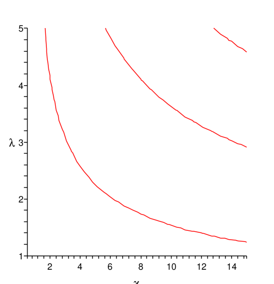
Figure 5: The first three solutions $\lambda$ to Eq. (100), showing the dependence on $\chi=\tau_{0}/\xi_{0}$.

We shall denote the minimum solution to this equation in $(1,\infty)$ by $\lambda_{0}$ (see Fig. 5); clearly $\lambda_{0}$ depends only on the ratio of the sampling time $\tau_{0}$ to the acceleration scale $\xi_{o}$. Two limits are of interest. Firstly, when $\tau_{0}/\xi_{0}\ll 1$, one may show that $\lambda_{0}^{2}\sim\beta^{4}\xi_{o}^{4}/\tau_{0}^{4}$ where $\beta$ is as in Eq. (64). Thus we regain the usual short-timescale constraint Eq. (66). This supports the ‘usual assumption’ (see Fewster (2004) for references) that sampling at scales shorter than those determined by the acceleration or curvature is governed by the bound obtained for inertial curves in Minkowski space. On the other hand, if we take $\tau_{0}\gg\xi_{o}$, we see that $\lambda_{0}\to 1$, so

$${\mathscr{E}}\gtrsim-\frac{11}{320\pi^{2}\xi_{o}^{4}}$$ (101)

in this limit.

In fact, more can be said for the inextendible case $\tau_{0}=\infty$, because the approximations made to gain Eq. (91) are rather wasteful in this limit. Choose any $g\in C_{0}^{\infty}({(-1/2,1/2)})$ with $g(0)\not=0$ and define $g_{\tau_{0}}(\tau)=\tau_{0}^{-1/2}g(\tau/\tau_{0})$, denoting the corresponding sampling tensor ${\sf f}_{\tau_{0}}$. Then a simple change of variables argument applied to Eq. (84) shows that

$${\mathcal{Q}}^{\rm weak}_{\bm{M}}({\sf f}_{\tau_{0}},\omega_{\bm{M}})=\int_{-\infty}^{\infty}dv\,|\widehat{g}(v)|^{2}Q(v/\tau_{0})\,,$$ (102)

and the limit $\tau_{0}\to\infty$ may be taken under the integral sign to yield

$$\lim_{\tau_{0}\to\infty}{\mathcal{Q}}_{\bm{M}}({\sf f}_{\tau_{0}},\omega_{\bm{M}})=2\pi Q(0)\int_{-\infty}^{\infty}d\tau|g_{\tau_{0}}(\tau)|^{2}\,.$$ (103)

In particular, if $g$ has unit $L^{2}$-norm, we have

$$\liminf_{\tau_{0}\to\infty}\frac{1}{\tau_{0}}\int_{\gamma}\langle T_{ab}u^{a}u^{b}\rangle_{\omega}g(\tau/\tau_{0})^{2}\,d\tau\geq-\frac{11\alpha^{4}}{480\pi^{2}}\,,$$ (104)

where $\alpha=\xi_{o}^{-1}$ is the proper acceleration of the curve, as asserted in Example 3 in the Introduction. Thus long term averages of the energy density measured along the curve are bounded from below, and no energy density can be less than this bound over the entire worldline. This is an improvement by a factor of $3/2$ over the bound given in Eq. (101). Using a more refined analysis one could presumably extract it as the limit of a result for general $\tau_{0}$, but we will not pursue this here. To summarise, we have reached the following conclusions.

Proposition III.3

Let ${\bm{N}}$ be a four-dimensional globally hyperbolic spacetime containing a timelike curve $\gamma$ of proper duration $\tau_{0}$ and constant proper acceleration $\alpha$. If $\gamma$ may be enclosed in a c.e.g.h.s. of ${\bm{N}}$ which is causally isometric to a c.e.g.h.s. of Minkowski space then we have

$$\sup_{\gamma}\langle T_{{\bm{N}}\,ab}u^{a}u^{b}\rangle_{\omega}\geq-\frac{(20\lambda_{0}^{2}-9)\alpha^{4}}{320\pi^{2}}$$ (105)

for any Hadamard state $\omega$ of the massless Klein–Gordon field, where $\lambda_{0}$ is the smallest solution to Eq. (100) in $[1,\infty)$ and depends on $\alpha\tau_{0}$. If $\gamma$ has infinite proper duration, we also have the more stringent constraint Eq. (104).

III.3 Massless fields in two dimensions

So far, we have only utilised the locally covariant difference QEIs of Sec. II.5. For massless fields in two dimensions, however, we also have the absolute QEI developed by Flanagan and others, described in Sec. II.4, which are also known to be optimal bounds. In this subsection we briefly discuss how the results of the previous subsections may be sharpened and generalised in this context. In fact the formula for the QEI bound is sufficiently simple that we may work directly in curved spacetime, rather than in Minkowskian subregions.

Let $\gamma:I\to{\bm{N}}$ be a smooth future-directed timelike curve, with velocity $u^{a}$ and accleration $a^{c}$ in a two-dimensional globally hyperbolic spacetime ${\bm{N}}$. As before, $I$ is an open interval of proper time. In order to apply Flanagan’s bound, we make the additional assumption that $\gamma$ may be enclosed within a c.e.g.h.s. ${\bm{N}}^{\prime}$ of ${\bm{N}}$, which is globally conformal to the whole of Minkowski space. Then Flanagan’s QEI asserts that

$$\int_{I}\langle T_{{\bm{N}}\,ab}u^{a}u^{b}\rangle_{\omega}(\gamma(\tau))g(\tau)^{2}\,d\tau\geq-\frac{1}{6\pi}\int_{I}\left[g^{\prime}(\tau)^{2}+g(\tau)^{2}\{R_{\bm{N}}(\gamma(\tau))-a^{c}(\tau)a_{c}(\tau)\}\right]\,d\tau$$ (106)

for all Hadamard states $\omega$ and any smooth, real-valued $g$ compactly supported in $I$, i.e., $g\in C_{0}^{\infty}({I;{\mathbb{R}}})$.

We proceed as above, obtaining the estimate

$${\mathscr{E}}\int_{I}g(\tau)^{2}\,d\tau\geq-\frac{1}{6\pi}\int_{I}\left[g^{\prime}(\tau)^{2}+g(\tau)^{2}\{R_{\bm{N}}(\gamma(\tau))-a^{c}(\tau)a_{c}(\tau)\}\right]\,d\tau\,,$$ (107)

for all $g\in C_{0}^{\infty}({I;{\mathbb{R}}})$, where ${\mathscr{E}}=\sup_{\gamma}\langle T_{{\bm{M}}\,ab}u^{a}u^{b}\rangle_{\omega}$ as usual. Converting to an eigenvalue problem, we deduce that

$${\mathscr{E}}\geq-\frac{\lambda_{0}}{6\pi}\,,$$ (108)

where $\lambda_{0}$ is the lowest element in the spectrum of the Friedrichs extension of the operator

$$(Lg)(\tau)=-g^{\prime\prime}(\tau)+(R_{\bm{N}}(\gamma(\tau))-a^{c}(\tau)a_{c}(\tau))g(\tau)\,,$$ (109)

on $C_{0}^{\infty}({I})$. Provided $R_{\bm{N}}$ and $a^{c}a_{c}$ are bounded along $\gamma$, the correct boundary conditions are Dirichlet conditions $g=0$ on $\partial I$ (see e.g., Fewster and Teo (2000)). We now give two illustrative examples.

Proposition III.4

Suppose ${\bm{N}}$ is a globally hyperbolic two-dimensional spacetime with a c.e.g.h.s. ${\bm{N}}^{\prime}$ which is globally conformal to the whole of Minkowski space. Then the following hold for all Hadamard states $\omega$ on ${\bm{N}}$:
(a) If $\gamma$ is a curve of proper duration $\tau_{0}$ contained in ${\bm{N}}^{\prime}$, with $R_{{\bm{N}}}-a^{c}a_{c}\equiv S$ constant along $\gamma$, then

$$\sup_{\tau\in I}\langle T_{{\bm{N}}\,ab}u^{a}u^{b}\rangle_{\omega}(\gamma(\tau))\geq\frac{S}{6\pi}-\frac{\pi}{6\tau_{0}^{2}}\,.$$ (110)

(b) If $\gamma:{\mathbb{R}}\to{\bm{N}}$ has (signed) proper acceleration growing linearly with proper time, $d\alpha/d\tau=p$, and $R_{\bm{N}}\equiv 0$ on $\gamma$, then

$$\sup_{\tau\in I}\langle T_{{\bm{N}}\,ab}u^{a}u^{b}\rangle_{\omega}(\gamma(\tau))\geq-\frac{|p|}{6\pi}\,.$$ (111)

The proof is straightforward: for (a), the eigenvalue problem is $-g^{\prime\prime}(\tau)=(\lambda+6\pi S)g(\tau)$ on an interval of length $\tau_{0}$ subject to Dirichlet boundary conditions, which easily yields the stated result. For (c), we may choose the origin of proper time so that $a^{c}a_{c}=-p^{2}\tau^{2}$ for some constant $p$. The eigenvalue problem is then

$$-g^{\prime\prime}(\tau)+p^{2}\tau^{2}g(\tau)=\lambda g(\tau)$$ (112)

which is the harmonic oscillator equation [and the Friedrichs extension is also the standard harmonic oscillator Hamiltonian]. The minimum value of $\lambda$ is therefore the ‘zero-point’ value $\lambda_{0}=|p|$. [The comparison with the usual quantum mechanical harmonic oscillator would correspond to units in which the mass and Planck’s constant are both set to $2$.] Thus we obtain the required result.

IV Calculations in specific spacetimes

In this section we illustrate our general method by some concrete calculations in a variety of locally Minkowskian spacetimes in both two and four dimensions. For the most part, we focus on the lower bounds, but upper bound calculations are included where they are enlightening. For each spacetime we consider, exact values of the renormalised stress-energy tensor are known (or easily obtained from existing results) for one or more states. This permits comparison with the results of our method.

IV.1 Two-dimensional timelike cylinder

Consider the massless scalar field on the two-dimensional timelike cylinder, ${\bm{C}}$, i.e., Minkowski space ${\bm{M}}_{2}$ quotiented by the group of translations $(t,x)\mapsto(t,x+nL)$ ($n\in{\mathbb{Z}}$). The Casimir vacuum $\omega_{\bm{C}}$ is the ground state of the scalar field on ${\bm{C}}$ (more precisely, it is a state on the algebra of first derivatives of the field–we will ignore this subtlety, which does not modify any of our conclusions below). The renormalized expectation value of the vacuum stress-tensor has the form

$$\langle T_{{\bm{C}}\,ab}\rangle_{\omega_{\bm{C}}}(x)=\rho_{\bm{C}}\left(\begin{array}[]{cc}1&0\\ 0&1\\ \end{array}\right),$$ (113)

where $\rho_{\bm{C}}$ is a constant. Our aim is to use quantum inequalities to provide upper and lower bounds on $\rho_{\bm{C}}$. The value of $\rho_{C}$ is, of course, well known, and will satisfy the bounds we now derive; our aim is to demonstrate how it may be bounded without direct calculation.

In order to apply our method, we must identify suitable globally hyperbolic subspacetimes of ${\bm{C}}$. For any $0<\tau_{0}\leq L$, we may define a timelike geodesic $\gamma:(0,\tau_{0})\to{\bm{C}}$ by $\gamma(\tau)=(\tau,0)$. Then the double cone ${\rm int}\,\left(J^{+}(\gamma(0))\cap J^{-}(\gamma(\tau))\right)$ is a causally embedded globally hyperbolic subspacetime of ${\bm{C}}$, containing $\gamma$. As this subspacetime is globally conformal to the whole of Minkowski space and the energy density is constant along $\gamma$, we have the lower bound

$$\rho_{\bm{C}}\geq-\frac{\pi}{6\tau_{0}^{2}}\,,$$ (114)

from Prop. III.4(a) (in the case $S=0$). This bound clearly becomes more stringent as $\tau_{0}$ is increased, so we obtain the best bound possible (within this method) by taking $\tau_{0}=L$. As shown in Fig. 6, the corresponding diamond is one for which the corners of the diamond just barely fail to touch on the back of the cylinder. This gives the final result

$$\rho_{\bm{C}}\geq-\frac{\pi}{6L^{2}}\,.$$ (115)

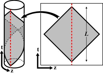
Figure 6: Diagram showing the “largest” causal diamond in two dimensional Minkowski space that can be isometrically embedded into the two dimensional cylinder spacetime with periodicity $L$ in the $z$-direction. To an observer inside the diamond in the cylinder spacetime, the quantum field theory and states would be indistinguishable from that in Minkowski space. The dashed vertical line is the worldline of a stationary observer.

We now demonstrate how to find an upper bound on $\rho_{\bm{C}}$ for which we must employ our locally covariant difference QWEI. Let $\widetilde{\gamma}$ be the curve $\widetilde{\gamma}(\tau)=(\tau,0)$ in ${\bm{M}}_{2}$ and let ${\bm{M}}^{\prime}={\rm int}\,J^{+}(\widetilde{\gamma}(0))\cap J^{-}(\widetilde{\gamma}(\tau_{0}))$, for some $0<\tau_{0}<L$, which is a c.e.g.h.s. of ${\bm{M}}_{2}$. Then the quotient map $q:{\bm{M}}_{2}\to{\bm{C}}$ defines a causal isometric embedding of ${\bm{M}}^{\prime}$ in ${\bm{C}}$, with $q({\bm{M}}^{\prime})$ equal to the double cone constructed earlier in this subsection. By Cor. II.4 we have

$$\langle T_{{\bm{C}}}(q_{*}{\sf f})\rangle_{\omega_{\bm{C}}}\leq{\mathcal{Q}}^{\rm weak}_{\bm{C}}({\sf f},\omega_{\bm{C}})$$ (116)

for any sampling tensor ${\sf f}\in{\mathscr{F}}_{{\bm{M}}^{\prime}}^{\rm weak}$. We define ${\sf f}$ by Eq. (49) for $g\in\widetilde{C}_{0}^{\infty}({(0,\tau_{0});{\mathbb{R}}})$ and then use the constancy of the energy density along $\gamma$ to find

$$\rho_{\bm{C}}\int_{0}^{\tau_{0}}g(\tau)^{2}\,d\tau\leq{\mathcal{Q}}^{\rm weak}_{\bm{C}}({\sf f},\omega_{\bm{C}})\leq\frac{1}{2\pi}\int(g^{\prime}(\tau))^{2}d\tau.$$ (117)

where the last inequality is derived in Appendix B. As usual, this may be converted into an eigenvalue problem: here, $\rho_{\bm{C}}\leq\lambda_{0}/(2\pi)$ where $\lambda_{0}=(\pi/\tau_{0})^{2}$ is the minimum eigenvalue of $-d^{2}/d\tau^{2}$ on $(0,\tau_{0})$ subject to Dirichlet boundary conditions. Combining with our earlier lower bound, we thus have

$$-\frac{\pi}{6L^{2}}\leq\rho_{\bm{C}}\leq\frac{\pi}{2L^{2}}.$$ (118)

The known value of $\rho_{\bm{C}}$ is exactly $-\pi/(6L^{2})$, see Birrell and Davies (1982), which, remarkably, saturates the lower bound. Thus we have shown that, in the cylinder spacetime, the Casimir vacuum energy density is the lowest possible static energy density compatible with the quantum energy inequalities. This however is not always the case, which we will see in later examples.

Because the energy density is in fact negative, the upper bound was not particularly enlightening in this example. However the situation is different for thermal equilibrium states. Let $\omega_{{\bm{C}},\beta}$ be the thermal equilibrium (KMS) state at inverse temperature $\beta$, relative to the static time translations. The stress-energy tensor is again diagonal

$$\langle T_{{\bm{C}}\,ab}\rangle_{\omega_{{\bm{C}},\beta}}(x)=\rho_{{\bm{C}},\beta}\left(\begin{array}[]{cc}1&0\\ 0&1\\ \end{array}\right),$$ (119)

where

$$\rho_{{\bm{C}},\beta}=-\frac{\pi}{6L^{2}}+\frac{\pi}{L^{2}}\sum_{n=1}^{\infty}\operatorname{cosech}^{2}\frac{n\pi\beta}{L}$$ (120)

see, e.g., Sec. 4.2 of Birrell and Davies (1982). By our general theory, these states should be constrained by the same lower bound as before, and this is evidently true, because the series contribution to $\rho_{{\bm{C}},\beta}$ is clearly positive. The upper bound depends on the temperature:

$$\rho_{{\bm{C}},\beta}\leq\frac{{\mathcal{Q}}^{\rm weak}_{{\bm{C}}}({\sf f},\omega_{{\bm{C}},\beta})}{\int_{0}^{\tau_{0}}g(\tau)^{2}\,d\tau}$$ (121)

for any $g\in\widetilde{C}_{0}^{\infty}({(0,\tau_{0});{\mathbb{R}}})$. In Appendix B we obtain the estimate

$${\mathcal{Q}}^{\rm weak}_{{\bm{C}}}({\sf f},\omega_{{\bm{C}},\beta})\leq\frac{{\mathcal{Q}}^{\rm weak}_{{\bm{C}}}({\sf f},\omega_{{\bm{C}}})}{1-e^{-2\pi\beta/L}}+\frac{\pi e^{\pi\beta/L}}{2L^{2}\sinh^{3}\pi\beta/L}\int_{-\infty}^{\infty}|g(\tau)|^{2}\,d\tau$$ (122)

and we may now immediately optimise over $g$ using our result for the ground state to obtain

$$-\frac{\pi}{6L^{2}}\leq\rho_{{\bm{C}},\beta}\leq\frac{\pi}{2L^{2}(1-e^{-2\pi\beta/L})}+\frac{\pi e^{\pi\beta/L}}{2L^{2}\sinh^{3}\pi\beta/L}$$ (123)

As shown in Fig. 7 this is consistent with the known value of $\rho_{{\bm{C}},\beta}$.

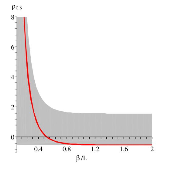
Figure 7: A graph showing the energy density $\rho_{{\bm{C}},\beta}$ in units of $L^{-2}$ of the thermal equilibrium state at temperature $\beta^{-1}$ on a cylinder of circumference $L$. The shaded region indicates the range permitted by the upper and lower bounds obtained from QEIs, illustrating Eq. (123).

IV.2 Spatial topology ${\mathbb{R}}^{3-j}\times{\mathbb{T}}^{j}$, $j=1,2,3$

Let us now consider various quotients of four-dimensional Minkowksi space by subgroups of the group of spatial translations. To begin, consider the quotient of four-dimensional Minkowski space, with inertial coordinates $(t,x,y,z)$ by the spatial translation subgroup $(t,x,y,z)\mapsto(t,x,y,z+nL_{1})$ ($n\in{\mathbb{Z}}$) for some fixed periodicity length $L_{1}>0$. We will denote the resulting spacetime by ${\bm{N}}_{1}$, and consider the ground state $\omega_{{\bm{N}}_{1}}$, which has a nonzero Casimir vacuum stress-energy tensor. A calculation using the method of images and the Minkowski space vacuum two-point function yields the renormalized vacuum stress-tensor for the massless scalar field in this spacetime, (see, e.g., DeWitt et al. (1979))

$${\langle T_{{\bm{N}}_{1}\,ab}\rangle}_{\omega_{{\bm{N}}_{1}}}=-\frac{\pi^{2}}{90L_{1}^{4}}\,{\rm diag}[\,1,\,-1,\,-1,\,3].$$ (124)

We will now show that this is consistent with the lower bound arising from the QEIs. To this end, let $\gamma(\tau)=(\tau,x_{0})$ for some fixed $x_{0}\in{\mathbb{R}}^{2}\times{\mathbb{T}}$. Then the double cone ${\rm int}\,\left(J^{+}(\gamma(0))\cap J^{-}(\gamma(L_{1}))\right)$ is a c.e.g.h.s. of ${\bm{N}}_{1}$ which is causally isometric to a double cone in Minkowski space. Thus the portion of $\gamma$ parametrised by $(0,L_{1})$ meets the hypotheses of Prop. III.1 and we have

$$\sup_{\gamma}\langle T_{{\bm{N}}_{1}\,00}\rangle_{\omega}\geq-\frac{C_{4}}{L_{1}^{4}}$$ (125)

for any Hadamard state $\omega$ of the Klein–Gordon field. In particular, the state $\omega_{{\bm{N}}_{1}}$ obeys this bound, as $\pi^{2}/90\approx 0.109662<C_{4}$. In fact the energy density is about thirty times smaller than the QEI bound in this case.

Thus the QEI bounds can be rather weak. But this is necessary, as can be seen from the next examples, in which the same lower bound must constrain a more negative energy density. Consider the spacetime ${\bm{N}}_{2}\cong{\mathbb{R}}\times{\mathbb{R}}\times{\mathbb{T}}^{2}$, which may be obtained by quotienting ${\bm{N}}_{1}$ by the translation group $(t,x,y,z)\mapsto(t,x,y+nL_{2},z)$ ($n\in{\mathbb{Z}}$) for some nonnegative $L_{2}$, which, without loss of generality, we take to be no less than $L_{1}$. Because $L_{2}\geq L_{1}$ we may apply Prop. III.1 to a double cone of the same size as before, so the lower bound is unchanged. However the stress tensor is now DeWitt et al. (1979)

$${\langle T_{{\bm{N}}_{2}\,ab}\rangle}_{\omega_{{\bm{N}}_{2}}}=-\frac{1}{2\pi^{2}L_{1}^{4}}\sum_{(m,n)\in{\mathbb{Z}}^{2}\backslash\{0\}}\frac{1}{(m^{2}+n^{2})^{2}}\,{\rm diag}[\,1,\,-1,\,1,\,1]$$ (126)

in the special case $L_{2}=L_{1}$. The sum can no longer be given in closed form, but numerically the overall prefactor (equal to the energy density on the worldline $\tau\mapsto(\tau,x_{0})$) is given in DeWitt et al. (1979) as $-0.305/L_{1}^{4}$. This is still consistent with Eq. (125), with energy density now only around ten times smaller than the bound.

In exactly the same way we may quotient ${\bm{N}}_{2}$ by the translation subgroup $(t,x,y,z)\mapsto(t,x+nL_{3},y,z)$ ($n\in{\mathbb{Z}}$), thereby forming ${\bm{N}}_{3}\cong{\mathbb{R}}\times{\mathbb{T}}^{3}$. If we again suppose that $L_{1}\leq L_{2}\leq L_{3}$, then the bound Eq. (125) still applies to the ground state on this spacetime. (Since this spacetime supports normalisable zero modes for the massless scalar field, one must regard this as a state on the algebra of derivatives of the field, much as for massless fields in two-dimensions). On the other hand, the stress-energy tensor in the natural ground state is

$${\langle T_{{\bm{N}}_{3}\,ab}\rangle}_{\omega_{{\bm{N}}_{3}}}=-\frac{1}{2\pi^{2}L_{1}^{4}}\sum_{(l,m,n)\in{\mathbb{Z}}^{3}\backslash\{0\}}\frac{1}{(l^{2}+m^{2}+n^{2})^{2}}\,{\rm diag}\left[\,1,\,\frac{1}{3},\,\frac{1}{3},\,\frac{1}{3}\right]$$ (127)

in the special case $L_{1}=L_{2}=L_{3}$. The energy density along $\tau\mapsto(\tau,x_{0})$ in this case is numerically computed to be $0.838/L_{1}^{4}$, which is again consistent with the QEI constraint Eq. (125), which is now weaker by a factor of less than $4$.

Let us note that the massless QEI bound also provides a lower bound on the ground state energy densities of massive scalar fields in these spacetimes. Consistency here is seen from the fact that the mass diminishes the magnitude of the energy density Tanaka and Hiscock (1995) (note the misprints in Tanaka and Hiscock (1995) noted in Langlois (2005) which do not, however, affect the final result).

IV.3 Misner Universe

Our third example concerns (the globally hyperbolic portion of) the Misner universe ${\bm{U}}$; namely, the quotient of $(0,\infty)\times{\mathbb{R}}^{3}$ with metric

$$ds^{2}=dt^{2}-t^{2}\left(dx^{1}\right)^{2}-\left(dx^{2}\right)^{2}-\left(dx^{3}\right)^{2}\,,$$ (128)

by the translation group $(t,x^{1},x^{2},x^{3})\mapsto(t,x^{1}+na,x^{2},x^{3})$ ($n\in{\mathbb{Z}}$) for some constant $a>0$. That is, the $x^{1}$ coordinate has been compactified onto a circle. We restrict to $t>0$ to avoid the closed null geodesics which would appear at $t=0$ and the closed timelike curves appearing for $t<0$. Under the coordinate transformation

$$y^{0}=t\cosh(x^{1}),\qquad y^{1}=t\sinh(x^{1}),\qquad y^{2}=x^{2},\qquad y^{3}=x^{3},$$ (129)

we may, equivalently, regard Misner space as the wedge $y^{0}>|y^{1}|$ of Minkowski spacetime with the points $(y^{0},y^{1},y^{2},y^{3})$ and $(y^{0}\cosh(na)+y^{1}\sinh(na),y^{1}\cosh(na)+y^{0}\sinh(na),y^{2},y^{3})$ identified for each $n\in{\mathbb{Z}}$.

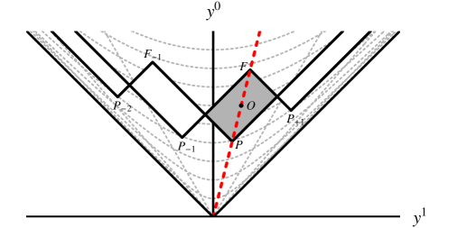
Figure 8: The covering space of the Misner universe is the wedge $y^{0}>|y^{1}|$ of Minkowski spacetime, shown here in cross section in the $y^{0}$-$y^{1}$ coordinates. Points in the covering space are identified, as described in the text, along the background hyperbolæ. Also shown is a stationary geodesic in the Misner universe, which in the covering space is a constant velocity observer (dashed line). For such an observer, the largest causal diamond for a given center point that is isomorphic to a subset of Minkowski space is shown in gray. Identified images of this diamond are also shown in white.

Define a curve $\gamma(\tau)=(\tau,{\bm{x}}_{o})$ in the original coordinates, for some constant $x_{0}\in{\mathbb{T}}\times{\mathbb{R}}^{2}$. This is a timelike geodesic, with velocity $u^{a}=(1,\bm{0})$. In the Minkowski space cover, this worldline is given by

$$\gamma(\tau)=\left(\begin{array}[]{c}\tau\cosh(x_{o}^{1})\\[3.0pt] \tau\sinh(x_{o}^{1})\\[3.0pt] x_{o}^{2}\\[3.0pt] x_{o}^{3}\end{array}\right)\qquad\mbox{ with }\qquad u^{a}(\tau)=\left(\begin{array}[]{c}\cosh(x_{o}^{1})\\[3.0pt] \sinh(x_{o}^{1})\\[3.0pt] 0\\[3.0pt] 0\end{array}\right),$$ (130)

which is a constant velocity geodesic, as shown by the bold dashed line in Figure 8. Let us consider a portion of this curve, running between $P=\gamma(\tau_{P})$ and $F=\gamma(\tau_{F})$, which is such that ${\rm int}(J^{+}(P)\cap J^{-}(F))$ is a c.e.g.h.s. of Misner space isometric to a double cone in Minkowski space. Assuming that this region is maximal, it must be that the geodesic joining the $n=+1$ image $P_{+1}$ of $P$ to $F$ is null. Setting $\tau_{O}=(\tau_{F}+\tau_{P})/2$ and $L=(\tau_{F}-\tau_{P})/2$, this yields the condition

$$\left[\left(\tau_{O}+\frac{L}{2}\right)\cosh(x_{o}^{1})-\left(\tau_{O}-\frac{L}{2}\right)\cosh(x_{o}^{1}+a)\right]^{2}-\left[\left(\tau_{O}+\frac{L}{2}\right)\sinh(x_{o}^{1})-\left(\tau_{O}-\frac{L}{2}\right)\sinh(x_{o}^{1}+a)\right]^{2}=0,$$ (131)

which entails

$$L=2\tau_{O}\tanh\left(\frac{a}{2}\right).$$ (132)

This is the largest double cone of this type, centered on $O$, in which an observer cannot detect the compactified nature of the $x^{1}$-direction. We may therefore apply Prop. III.1 to the portion $\gamma_{PF}$ of $\gamma$ lying between $P$ and $F$. This gives

$$\sup_{\gamma_{PF}}\langle T_{{\bm{U}}\,ab}u^{a}u^{b}\rangle_{\omega}\geq-\frac{C_{4}}{L^{4}}=-\frac{C_{4}}{(2\tau_{O}\tanh(a/2))^{4}}$$ (133)

for any Hadamard state $\omega$ on Misner space. In particular, an energy density $\rho(\tau)=\langle T_{{\bm{U}}\,ab}u^{a}u^{b}\rangle_{\omega}(\gamma(\tau))$ of the form $\rho(\tau)=-C/\tau^{4}$, for which $\sup_{\gamma}\rho=-C/\tau_{F}^{4}$, would be subject to the constraint

$$C\leq\frac{C_{4}}{16}\left(2+\coth(a/2)\right)^{4}.$$ (134)

By adapting the eigenvalue method, we may obtain a better bound. Let us suppose that $\rho$ obeys

$$\rho(\tau)\leq\frac{K}{16\pi^{2}\tau^{4}}$$ (135)

on $I=(\tau_{O}-L/2,\tau_{0}+L/2)$. Then by exactly the same arguments as in Sec. III.1, we may deduce

$$K\geq-\inf_{g}\frac{\int|g^{\prime\prime}(\tau)|^{2}d\tau}{\int\tau^{-4}|g(\tau)|^{2}d\tau}.$$ (136)

where the $\tau^{-4}$ in the denominator comes from the form of $\rho$, and the infimum is taken over all $g\in C_{0}^{\infty}({I})$. The denominator can be reinterpreted as the norm of $g$ in $L^{2}(I,\tau^{-4}d\tau)$. Integrating by parts twice, we may rewrite the numerator as $-{\langle g\mid Lg\rangle}$ where the inner product is that of $L^{2}(I,\tau^{-4}d\tau)$ and $L$ is defined on $C_{0}^{\infty}({I})$ by

$$(Lg)(\tau)=\tau^{4}g^{\prime\prime\prime\prime}(\tau)$$ (137)

and is symmetric, i.e., ${\langle h\mid Lg\rangle}={\langle Lh\mid g\rangle}$ for all $g,h\in C_{0}^{\infty}({I})$. The minimisation problem is then solved by finding the lowest spectral point of the Friedrichs extension of $L$. It may be shown that the Friedrichs extension again amounts to the imposition of Dirichlet boundary conditions $g=g^{\prime}=0$ on $\partial I$ , and the problem now reduces to the study of the ODE

$$g^{\prime\prime\prime\prime}(\tau)-\frac{\lambda}{\tau^{4}}g(\tau)=0.$$ (138)

Again we wish to determine the minimum eigenvalue $\lambda$ for eigensolutions that satisfy the boundary conditions. The substitution $g(\tau)=h(\frac{1}{2}\ln(\tau))$ converts the equation to a constant coefficient linear equation, and one may determine the general solution (e.g., using Mathematica) as

$$h(l)=c_{1}e^{3l}\cos\left(l\sqrt{4\sqrt{\lambda+1}-5}\right)+c_{2}e^{3l}\sin\left(l\sqrt{4\sqrt{\lambda+1}-5}\right)+c_{3}e^{\left(3+\sqrt{4\sqrt{\lambda+1}+5}\right)l}+c_{4}e^{\left(3-\sqrt{4\sqrt{\lambda+1}+5}\right)l},$$ (139)

where $(c_{1},c_{2},c_{3},c_{4})$ are constants. Imposing three of the boundary conditions fixes three of the constants in terms of the fourth, which serves as an overall magnitude for the test function. The fourth boundary condition can then be used to determine the eigenvalues. A somewhat involved calculation leads to the transcendental equation to determine $\lambda$ implicitly in terms of $a$:

$$\frac{\sqrt{16\lambda-9}}{5}=\frac{\sin\left(\frac{a}{2}\sqrt{4\sqrt{\lambda+1}-5}\right)\sinh\left(\frac{a}{2}\sqrt{4\sqrt{\lambda+1}+5}\right)}{\cos\left(\frac{a}{2}\sqrt{4\sqrt{\lambda+1}-5}\right)\cosh\left(\frac{a}{2}\sqrt{4\sqrt{\lambda+1}+5}\right)-1}.$$ (140)

We denote $\lambda$, so determined, as $\lambda(a)$; this constrains our original value $K$ by

$$K\geq-\lambda(a).$$ (141)

Our interest in energy densities proportional to $\tau^{-4}$ stems from the state constructed by Hiscock and Konkowski Hiscock and Konkowski (1982). This quasifree state, which we denote $\omega_{\bm{U}}$, is obtained by applying the method of images to the Minkowski space two-point function in the wedge $y^{0}>|y^{1}|$, and then carrying it back to the original Misner coordinates to find the renormalized vacuum expectation value of the stress-tensor. Hiscock and Konkowski considered the conformally coupled scalar field, but their calculations can be easily reproduced in the minimally-coupled case, to yield

$${\langle T_{{\bm{U}}\,ab}\rangle}_{\omega_{\bm{U}}}(t)=\frac{K(a)}{16\pi^{2}\,t^{4}}\,\mbox{diag}\left[1,3t^{2},-1,-1\right],$$ (142)

where

$$K(a)=-\sum_{n=1}^{\infty}\operatorname{cosech}^{4}\left(\frac{na}{2}\right)$$ (143)

is a negative constant depending on the $x^{1}$-period $a$ . Both the coefficient $K(a)$ and the numerical evaluation of the lower bound $-\lambda(a)$ are plotted in Fig. 9. It is obvious that $K(a)$, and thus the energy density obey the QEI constraint for all values of $a$. The bound Eq. (134) is still weaker.

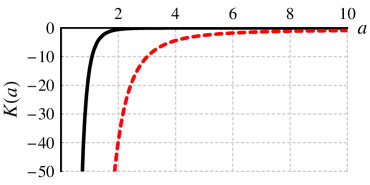
Figure 9: The numerical factor $K(a)$ for the vacuum stress tensor in the Misner universe (solid line) plotted for a range of the closure scale $a$. Also shown is the lower bounds from $-\lambda(a)$ (dashed line). The lower bound from Eq. (134) is so weak (it asymptotically approaches $\sim-2500$ from below for large $a$) that it is not included to preserve detail in the figure above.

IV.4 Rindler spacetime

The Rindler spacetime ${\bm{R}}$ is the “right wedge” of Minkowski space, i.e., the region $\left\{(t,x,y,z)\in{\mathbb{R}}^{4}:\mbox{ s.t. }x>|t|\right\}$ in inertial coordinates $(t,x,y,z)$. We may also make the coordinate transformation

$$\begin{array}[]{ccl}t=\xi\sinh(\eta),&&y=y,\\[4.0pt] x=\xi\cosh(\eta),&&z=z,\end{array}$$ (144)

to obtain the metric in the form

$$ds^{2}=\xi^{2}d{\eta}^{2}-d{\xi}^{2}-d{y}^{2}-d{z}^{2},$$ (145)

with coordinate ranges $\eta,y,z\in{\mathbb{R}}$, $\xi\in(0,\infty)$. Lines of constant $\xi$, when mapped into Minkowski space, are worldlines for observers undergoing constant proper acceleration $\alpha=\xi^{-1}$. Rindler spacetime is static with respect to $\eta$ (corresponding to Lorentz invariance in the $xt$ plane) and is invariant under Euclidean transformations of the $yz$ plane.

Clearly any line of constant $\xi$ meets the conditions of Prop. III.3 and we may immediately read off that any static Hadamard state $\omega$ on ${\bm{R}}$ must obey

$${\langle T_{{\bm{R}}\,ab}u^{a}u^{b}\rangle}_{\omega}(\eta,\xi,y,z)\geq-\frac{11}{480\pi^{2}\xi^{4}}$$ (146)

where $u^{a}$ is the unit vector parallel to $\partial/\partial\eta$. In particular, this provides a constraint on the energy density $\rho_{\bm{R}}=\langle T_{{\bm{R}}\,ab}u^{a}u^{b}\rangle_{\omega_{{\bm{R}}}}$ in the ground state $\omega_{\bm{R}}$ (which is Hadamard). This may also be computed exactly: it was first computed for the conformally coupled scalar field by Candelas and Deutsch Candelas and Deutsch (1977) and one can easily generalize their results to the minimally coupled scalar field to obtain 

$$\rho_{\bm{R}}=-\frac{11}{480\pi^{2}\xi_{o}^{4}},$$ (147)

which is exactly the lower bound given above. Thus, remarkably, the Rindler ground state saturates the QEI constraints, which were obtained using local covariance and the Minkowski vacuum, and nowhere involved $\omega_{\bm{R}}$.

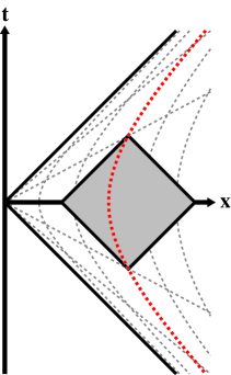
Figure 10: Diagram showing Rindler spacetime (with the two perpendicular space dimensions suppressed) embedded into Minkowski spacetime. The dashed hyperbolic line, the worldline of a constantly accelerating observer, is the image of a constant $\xi$ observer’s worldline in Rindler coordinates. The grey diamond is a causal region that can be isometrically identified between the two “different” coordinate systems.

Let us also examine how an upper bound might be obtained. Let $\gamma(\tau)=(\tau/\xi_{o},\xi_{o},0,0)$ in $(\eta,\xi,y,z)$ coordinates and set ${\sf u}=\dot{\gamma}$ as usual. We consider sampling along $\gamma$, with sampling tensors of form

$${\sf f}({\sf t})=\int t_{ab}|_{\gamma(\tau)}u^{a}u^{b}g(\tau)^{2}\,d\tau$$ (148)

for $g\in\widetilde{C}_{0}^{\infty}({{\mathbb{R}};{\mathbb{R}}})$. Since the energy density is constant along $\gamma$, the upper bound of Cor. II.4 gives

$$\rho_{\bm{R}}\int g(\tau)^{2}\,d\tau=\langle{\sf T}_{\bm{R}}({\sf f})\rangle_{\omega_{\bm{R}}}\leq{\mathcal{Q}}^{\rm weak}_{\bm{R}}({\sf f},\omega_{\bm{R}})\,.$$ (149)

The right-hand side can be read off from the difference QEI derived by Pfenning Pfenning (2002) for the electromagnetic field, because the corresponding bound for the scalar field is exactly half of the electromagnetic expression :

$${\mathcal{Q}}^{\rm weak}_{\bm{R}}({\sf f},\omega_{\bm{R}}) = \frac{1}{16\pi^{3}}\int_{0}^{\infty}\left|\widehat{g}(u)\right|^{2}\left(u^{4}+2\xi_{o}^{-2}u^{2}\right)du$$ (150)

$$= \frac{1}{16\pi^{2}}\int_{-\infty}^{\infty}\left(\left|g^{\prime\prime}(\tau)\right|^{2}+2\xi_{o}^{-2}\left|g^{\prime}(\tau)\right|^{2}\right)d\tau\,.$$

Next consider scaling the test function, replacing $g$ by $g_{\alpha}(\tau)=\alpha^{-1/2}g(\tau/\alpha)$. We find, considering the scaling behavior of the above expression,

$$\rho_{\bm{R}}\leq\frac{1}{16\pi^{2}}\frac{\int\left(|g^{\prime\prime}(\tau)|^{2}+2\alpha^{2}\xi_{o}^{-2}|g^{\prime}(\tau)|^{2}\right)d\tau}{\alpha^{4}\int g(\tau)^{2}d\tau}$$ (151)

for which the right hand side vanishes in the limit of $\alpha\rightarrow\infty$. Thus we find consistency with the known fact that the expectation value of the Rindler ground state is bounded above by zero, i.e. $\rho_{\bm{R}}\leq 0$.

V Summary

In this paper we have initiated the study of interrelations between quantum energy inequalities and local covariance. We have formulated definitions of locally covariant QEIs, and shown that existing QEIs obey them, modulo small additional restrictions (Sec. II). The main thrust of our work has been directed at providing a priori constraints on renormalised energy densities in locally Minkowskian regions, accomplished in Sec. III. The simple geometric nature of these bounds makes them easy to apply in practice, and a number of future applications are envisaged. In particular, we will discuss applications to the Casimir effect in a companion paper Fewster and Pfenning ; at the theoretical level, it is possible to place the present discussion in the categorical language of Brunetti et al. (2003), and this will be done elsewhere. Equally important are the specific calculations reported in Sec. IV. Here we saw that, in some situations, the QEI bounds give best-possible constraints on the energy density, and that typical ground state energy densities are not over-estimated by the QEI bound by more than a factor of about $30$ at worst (in the examples so far studied).

Finally, although we confined our attention largely to locally Minkowskian spacetimes in Secs. III and IV, we emphasise again that other interesting cases may be studied using our general formalism, as, for example, in the work of Marecki Marecki on spacetimes with locally Schwarzschild subregions.

Appendix A The locally covariant quantum field theory of a scalar field

In this appendix we describe the construction of the quantised Klein–Gordon field within the algebraic approach to quantum field theory, and explain the construction of pulled back states used in Sec. II.2.

The free scalar field of mass $m\geq 0$ may be quantised on any globally hyperbolic spacetime ${\bm{M}}$ in the sense that one may construct a complex unital $*$-algebra ${\mathfrak{A}}({\bm{M}})$ whose elements may be interpreted as ‘polynomials in smeared fields’. A typical element of the algebra is a complex linear combination of the identity 11 and a finite number of terms each of which is a finite product of a number of objects $\Phi_{\bm{M}}(f)$ where $f$ is a test function (i.e., smooth and compactly supported) on $M$. The algebra also satisfies a number of relations:

1. $\Phi_{\bm{M}}(\lambda f+\mu g)=\lambda\Phi_{\bm{M}}(f)+\mu\Phi_{\bm{M}}(g)$

2. $\Phi_{\bm{M}}(f)^{*}=\Phi_{\bm{M}}(\overline{f})$

3. $\Phi_{\bm{M}}((\Box+m^{2})f)=0$

4. $[\Phi_{\bm{M}}(f),\Phi_{\bm{M}}(g)]=iE_{{\bm{M}}}(f,g)\leavevmode\hbox{\rm{\small 1\kern-3.8pt\normalsize 1}}$

for all test functions $f,g$ on $M$ and complex scalars $\lambda,\mu$, where $E_{{\bm{M}}}$ is the advanced-minus-retarded fundamental solution to $\Box+m^{2}$ on ${\bm{M}}$. The first two axioms are necessary for compatibility with the idea of $\Phi_{\bm{M}}(f)$ as a smeared hermitian field; the third expresses the field equation in ‘weak’ form; the fourth expresses the commutation relations.

Now let $\psi$ be a causal isometric embedding of ${\bm{M}}_{1}$ into ${\bm{M}}_{2}$. Any test function $f$ on $M_{1}$ now corresponds to a test function $\psi_{*}f$ on $M_{2}$, defined by $(\psi_{*}f)(x)=f(\psi^{-1}(x))$ for $x\in\psi(M_{1})$ and $(\psi_{*}f)(x)=0$ otherwise. We may use this to define a map $\alpha_{\psi}$ between ${\mathfrak{A}}({\bm{M}}_{1})$ and ${\mathfrak{A}}({\bm{M}}_{2})$ such that

1. $\alpha_{\psi}\leavevmode\hbox{\rm{\small 1\kern-3.8pt\normalsize 1}}_{{\mathfrak{A}}({\bm{M}}_{1})}=\leavevmode\hbox{\rm{\small 1\kern-3.8pt\normalsize 1}}_{{\mathfrak{A}}({\bm{M}}_{2})}$

2. $\alpha_{\psi}(\Phi_{{\bm{M}}_{1}}(f))=\Phi_{{\bm{M}}_{2}}(\psi_{*}f)$ for all test functions $f$ on $M_{1}$

3. $\alpha_{\psi}$ extends to general elements of ${\mathfrak{A}}({\bm{M}}_{1})$ as a $*$-homomorphism, i.e., $\alpha_{\psi}$ is linear and obeys $\alpha_{\psi}(AB)=\alpha_{\psi}(A)\alpha_{\psi}(B)$ and $\alpha_{\psi}(A^{*})=\alpha_{\psi}(A)^{*}$ for all $A,B\in{\mathfrak{A}}({\bm{M}}_{1})$.

In the body of the text we have used the notation $\psi_{*}$ for $\alpha_{\psi}$, relying on the context for the appropriate meaning; here, it is convenient to distinguish the two maps. One must check that the last statement is compatible with the axioms stated above–the only nontrivial one is the commutation relation, where the causal nature of $\psi$ plays a key role and guarantees that $\alpha_{\psi}$ is well-defined. What needs to be proved boils down to checking that

$$E_{{\bm{M}}_{1}}(f,g)=E_{{\bm{M}}_{2}}(\psi_{*}f,\psi_{*}g)$$ (152)

for all test functions $f,g$ on $M_{1}$. This equivalence is proved as follows. Writing $E^{\pm}_{{\bm{M}}}$ for the advanced ($-$) and retarded $(+)$ Green functions on ${\bm{M}}$, $E^{\pm}_{{\bm{M}}_{2}}\psi_{*}f$ solves the inhomogeneous Klein–Gordon equation on ${\bm{M}}_{2}$ with source $\psi_{*}f$ and support in $J^{\pm}_{{\bm{M}}_{2}}({\rm supp}\,f)$. Because $\psi$ is a causal isometry, the pull-back $\psi^{*}E^{\pm}_{{\bm{M}}_{2}}\psi_{*}f$ solves the inhomogeneous Klein–Gordon equation on ${\bm{M}}_{1}$ with source $f$ and support in $J^{\pm}_{{\bm{M}}_{1}}({\rm supp}\,f)$; by uniqueness of solution, we have $E_{{\bm{M}}_{1}}^{\pm}f=\psi^{*}E_{{\bm{M}}_{2}}^{\pm}\psi_{*}f$. Accordingly $\psi_{*}E_{{\bm{M}}_{1}}=E_{{\bm{M}}_{2}}\psi_{*}$ and the required result follows.

In the algebraic approach we have been pursuing, a state of the quantum field on ${\bm{M}}$ is a linear map $\omega$ from ${\mathfrak{A}}({\bm{M}})$ to the complex numbers, obeying $\omega(\leavevmode\hbox{\rm{\small 1\kern-3.8pt\normalsize 1}})=1$ and $\omega(A^{*}A)\geq 0$ for any $A\in{\mathfrak{A}}({\bm{M}})$. One interprets $\omega(A)$ as the expectation value of observable $A$ in state $\omega$. In particular, each state yields a hierarchy of $n$-point functions, i.e., maps of the form

$$(f_{1},\ldots,f_{n})\mapsto\omega(\Phi_{\bm{M}}(f_{1})\cdots\Phi_{\bm{M}}(f_{n}))\,;$$ (153)

we will restrict attention to those states whose corresponding $n$-point functions are distributions. A state $\omega$ is Hadamard if its two-point function has a particular singular structure which is determined by the local metric and causal properties of the spacetime. Note that none of the structure introduced so far invokes any particular Hilbert space representation of the theory.

Now suppose again that $\psi$ is a causal isometric embedding of ${\bm{M}}_{1}$ into ${\bm{M}}_{2}$ and let $\omega_{2}$ be a state on ${\mathfrak{A}}({\bm{M}}_{2})$. We obtain a state $\omega_{1}$ on ${\mathfrak{A}}({\bm{M}}_{2})$ by

$$\omega_{1}(A)=\omega_{2}(\alpha_{\psi}(A))$$ (154)

for any $A\in{\mathfrak{A}}({\bm{M}}_{1})$; that is, $\omega_{1}=\alpha_{\psi}^{*}\omega_{2}$, where $\alpha_{\psi}^{*}$ is the dual map to $\alpha_{\psi}$ (in the body of the text, we have written $\psi^{*}$ for $\alpha_{\psi}^{*}$). The $n$-point functions are therefore related by

$$\omega_{1}(\Phi_{{\bm{M}}_{1}}(f_{1})\cdots\Phi_{{\bm{M}}_{1}}(f_{n}))=\omega_{2}(\alpha_{\psi}(\Phi_{{\bm{M}}_{1}}(f_{1})\cdots\Phi_{{\bm{M}}_{1}}(f_{n})))=\omega_{2}(\Phi_{{\bm{M}}_{2}}(\psi_{*}f_{1})\cdots\Phi_{{\bm{M}}_{2}}(\psi_{*}f_{n}))\,.$$ (155)

It is useful to write this in ‘unsmeared’ notation. Let $w_{j}^{(n)}$ be the $n$-point functions of $\omega_{j}$. Then the last equation becomes

$$\int_{M_{1}}d{\rm vol}_{{\bm{g}}_{1}}(x_{1})\cdots\int_{M_{1}}d{\rm vol}_{{\bm{g}}_{1}}(x_{n})\,w_{1}^{(n)}(x_{1},\ldots,x_{n})f_{1}(x_{1})\cdots f_{n}(x_{n})$$ (156)

$$= \int_{M_{2}}d{\rm vol}_{{\bm{g}}_{2}}(y_{1})\cdots\int_{M_{2}}d{\rm vol}_{{\bm{g}}_{2}}(y_{n})\,w_{2}^{(n)}(y_{1},\ldots,y_{n})\psi_{*}f_{1}(y_{1})\cdots\psi_{*}f_{n}(y_{n})$$

$$= \int_{M_{1}^{\times n}}d{\rm vol}_{{\bm{g}}_{1}}(x_{1})\cdots\,d{\rm vol}_{{\bm{g}}_{1}}(x_{n})w_{1}^{(n)}(\psi(x_{1}),\ldots,\psi(x_{n}))f_{1}(x_{1})\cdots f_{n}(x_{n})\,,$$

where the change of variables employed in the last step is justified by the fact that $\psi$ is an isometry. As this holds for all choices of $f_{k}$, we may deduce that

$$w_{1}^{(n)}(x_{1},\ldots,x_{n})=w_{2}^{(n)}(\psi(x_{1}),\ldots,\psi(x_{n}))\,;$$ (157)

that is, the $n$-point functions of $\omega_{1}$ are the pull-backs by $\psi$ of those of $\omega_{2}$. It follows that if $\omega_{2}$ is Hadamard then so too is $\omega_{1}$, because the two-point function is simply pulled back under $\psi$ and the Hadamard series is constructed from the local causal and metric structure which is preserved under $\psi$. Since the stress-energy tensor is renormalised by subtracting the first few terms of the Hadamard series from the two point function, and then taking suitable derivatives before taking the coincidence limit (making a further locally constructed correction to ensure conservation of the stress tensor), we have the following important consequence, which we isolate as a theorem.

Theorem A.1

Suppose $\psi$ is a causal isometric embedding of globally hyperbolic spacetime ${\bm{M}}_{1}$ in a globally hyperbolic spacetime ${\bm{M}}_{2}$. Any Hadamard state of the massive Klein–Gordon quantum field on ${\bm{M}}_{2}$ induces a Hadamard state of the same theory on ${\bm{M}}_{1}$, whose $n$-point functions and renormalised expected stress-energy tensor are the pull-backs by $\psi$ of the corresponding quantities on ${\bm{M}}_{2}$.

This fits in with the principle that one should not be able to tell, by local experiments, whether one is in ${\bm{M}}_{1}$ or its image within the larger spacetime ${\bm{M}}_{2}$. It also justifies us in the abuse of notation perpetrated in Sec. II.2, where we wrote $\psi^{*}$ in place of $\alpha_{\psi}^{*}$, and (dually) $\psi_{*}$ in place of $\alpha_{\psi}$.

Let us conclude by briefly describing more of the structure set out by Brunetti et al. (2003). The key is the observation that the globally hyperbolic spacetimes of given dimension form the objects of a category in which the morphisms are causal isometric embeddings. One may also consider a category of unital $*$-algebras with injective unit-preserving $*$-homomorphisms as morphisms. The association of a globally hyperbolic spacetime ${\bm{M}}$ with the corresponding algebra ${\mathfrak{A}}({\bm{M}})$ is then shown to be a covariant functor between these categories and gives a precise meaning to the notion of ‘the same field theory on different spacetimes’ (and the same would be true even for theories not necessarily described in terms of a Lagrangian). A similar functorial description may be given to the association of the state space of the theory, and quantum fields are reinterpreted as natural transformations between functors. We refer the reader to Brunetti et al. (2003) for full details.

Appendix B Derivation of Scalar Field Quantum Weak Energy Inequality in the Cylinder Spacetime

In this appendix, we calculate quantum weak energy inequalities for the massless, minimally–coupled real scalar field in the two dimensional cylinder spacetime relative to the ground and thermal equilibrium states. We use the notation of Sec. IV.1.

The KMS state $\omega_{{\bm{C}},\beta}$ at inverse temperature $\beta$ has two-point function (see, e.g., Eq. (2.43) of Fulling and Ruijsenaars (1987))

$$w_{2,\beta}(x,x^{\prime})=\frac{1}{2L}\sum_{n\in{\mathbb{Z}}\backslash\{0\}}\frac{e^{ik_{n}(z-z^{\prime})}}{\omega_{n}(1-e^{-\beta\omega_{n}})}\,\left(e^{-i\omega(t-t^{\prime})}+e^{-\beta\omega_{n}}e^{i\omega(t-t^{\prime})}\right),$$ (158)

where $k_{n}=2\pi n/L$ and $\omega_{n}=|k_{n}|$, and the sum converges in the distributional sense (i.e., after smearing each term with test functions, the resulting series converges and its sum depends continuously on the test functions). We exclude the zero mode $n=0$ as usual, regarding $\omega_{{\bm{C}},\beta}$ as a state on the derivative fields. The two-point function of the ground state $\omega_{\bm{C}}$ is obtained as the zero temperature ($\beta\to\infty$) limit of this expression. We will be interested in the static curve $\gamma(\tau)=(\tau,0)$, and employ the tetrad $e_{0}=\partial/\partial t$, $e_{1}=\partial/\partial z$, which is invariant under Fermi–Walker transport along $\gamma$.

Following the procedure of Sec. II.5, we find

$$Q_{\gamma,\omega_{{\bm{C}},\beta}}(u)=\frac{1}{2\pi^{2}}\int_{(-\infty,u)}dv\,\widehat{T}_{\gamma,\omega_{{\bm{C}},\beta}}(v)$$ (159)

and

$$T_{\gamma,\omega_{{\bm{C}},\beta}}(\sigma)=\frac{1}{L}\sum_{n=1}^{\infty}\frac{\omega_{n}}{1-e^{-\beta\omega_{n}}}\left(e^{-i\omega_{n}\sigma}+e^{-\beta\omega_{n}}e^{i\omega_{n}\sigma}\right)\,.$$ (160)

Taking the Fourier transform, we have

$$\widehat{T}_{\gamma,\omega_{{\bm{C}},\beta}}(v)=\frac{2\pi}{L}\sum_{n=1}^{\infty}\frac{\omega_{n}}{1-e^{-\beta\omega_{n}}}\left(\delta(v-\omega_{n})+e^{-\beta\omega_{n}}\delta(v+\omega_{n})\right)$$ (161)

and therefore obtain

$$Q_{\gamma,\omega_{{\bm{C}},\beta}}(u)=\frac{1}{\pi L}\left\{\sum_{\begin{subarray}{c}n\in{\mathbb{N}}\\ {\rm s.t.}\omega_{n}<u\end{subarray}}\frac{\omega_{n}}{1-e^{-\beta\omega_{n}}}+\sum_{\begin{subarray}{c}n\in{\mathbb{N}}\\ {\rm s.t.}-\omega_{n}<u\end{subarray}}\frac{\omega_{n}e^{-\beta\omega_{n}}}{1-e^{-\beta\omega_{n}}}\right\}\,.$$ (162)

Note that $Q_{\gamma,\omega_{{\bm{C}},\beta}}$ is supported on ${\mathbb{R}}^{+}$ in the $\beta=\infty$ case, but otherwise on the whole of ${\mathbb{R}}$, albeit exponentially suppressed on the negative half line.

To arrive at convenient QEI bounds we estimate $Q_{\gamma,\omega_{{\bm{C}},\beta}}$ by

$$Q_{\gamma,\omega_{{\bm{C}},\beta}}(u)\leq Q_{\gamma,\omega_{{\bm{C}},\beta}}(0)+\frac{\vartheta(u)}{\pi L(1-e^{-2\pi\beta/L})}\sum_{\begin{subarray}{c}n\in{\mathbb{N}}\\ {\rm s.t.}\omega_{n}<u\end{subarray}}\omega_{n}$$ (163)

where $\vartheta$ is the Heaviside step function. To see that this estimate is valid, we note that $Q_{\gamma,\omega_{{\bm{C}},\beta}}(u)$ is clearly increasing on the negative half-line, so it is valid to bound it by $Q_{\gamma,\omega_{{\bm{C}},\beta}}(0)$ on $u\leq 0$; the second term in the estimate arises by noting that $(1-e^{-\beta\omega_{n}})^{-1}\leq(1-e^{-2\pi\beta/L})^{-1}$ for all $n$. Using this estimate again, we also have

$$Q_{\gamma,\omega_{{\bm{C}},\beta}}(0)=\sum_{n\in{\mathbb{N}}}\frac{\omega_{n}e^{-\beta\omega_{n}}}{1-e^{-\beta\omega_{n}}}\leq\frac{1}{\pi L(1-e^{-2\pi\beta/L})}\sum_{n=1}^{\infty}\frac{2\pi n}{L}e^{-2\pi\beta n/L}=\frac{e^{\pi\beta/L}}{4L^{2}\sinh^{3}\pi\beta/L}\,,$$ (164)

while, for $u>0$

$$\frac{1}{\pi L}\sum_{\begin{subarray}{c}n\in{\mathbb{N}}\\ {\rm s.t.}\omega_{n}<u\end{subarray}}\omega_{n}=\frac{1}{L^{2}}\tilde{n}(\tilde{n}+1)\leq\frac{2}{L^{2}}\tilde{n}^{2}\leq\frac{u^{2}}{2\pi^{2}}\,,$$ (165)

where $\tilde{n}$ is the greatest integer strictly less than $uL/(2\pi)$. Thus we have the estimate

$$Q_{\gamma,\omega_{{\bm{C}},\beta}}(u)\leq\frac{e^{\pi\beta/L}}{4L^{2}\sinh^{3}\pi\beta/L}+\frac{\vartheta(u)u^{2}}{2\pi^{2}(1-e^{-2\pi\beta/L})}\,.$$ (166)

It then follows that, in the notation of Sec. IV.1,

$${\mathcal{Q}}^{\rm weak}_{\bm{C}}({\sf f},\omega_{{\bm{C}},\beta}) = \int_{-\infty}^{\infty}du\,|\widehat{g}(u)|^{2}Q_{\gamma,\omega_{{\bm{C}},\beta}}(u)$$ (167)

$$\leq \frac{e^{\pi\beta/L}}{4L^{2}\sinh^{3}\pi\beta/L}\int_{-\infty}^{0}|\widehat{g}(u)|^{2}\,du+\frac{1}{2\pi^{2}(1-e^{-2\pi\beta/L})}\int_{0}^{\infty}u^{2}|\widehat{g}(u)|^{2}\,du$$

$$\leq \frac{\pi e^{\pi\beta/L}}{2L^{2}\sinh^{3}\pi\beta/L}\int_{-\infty}^{\infty}|g(\tau)|^{2}\,d\tau+\frac{1}{2\pi(1-e^{-2\pi\beta/L})}\int_{-\infty}^{\infty}|g^{\prime}(\tau)|^{2}\,d\tau$$ (168)

where we have used Parseval’s theorem and the fact that $|\widehat{g}(u)|$ is even for real-valued $g$ to convert the integral over ${\mathbb{R}}^{+}$ into one over ${\mathbb{R}}$. For the ground state, of course, this yields

$${\mathcal{Q}}^{\rm weak}_{\bm{C}}({\sf f},\omega_{{\bm{C}}})\leq\frac{1}{2\pi}\int_{-\infty}^{\infty}|g^{\prime}(\tau)|^{2}\,d\tau$$ (169)

and Eq. (122) follows immediately. Although our estimates are not very sharp, they have led to a very simple quantum inequality. In fact, for the ground state, this inequality is only $3$ times less restrictive than the optimal quantum inequality bound found in two dimensional Minkowski spacetime.

Appendix C A lemma concerning smooth functions

Recall from Sec. II.5 that we define $\widetilde{C}_{0}^{\infty}({I;{\mathbb{R}}})$ to be the set of smooth compactly supported real-valued functions $g$ on $I$ whose support is connected and which have no zeros of infinite order in the interior of that support (equivalently, $g$ has no zeros in $(\inf{\rm supp}\,g,\sup{\rm supp}\,g)$ of infinite order). Our aim is to prove the following result.

Lemma C.1

Let $g\in C_{0}^{\infty}({I;{\mathbb{R}}})$ and choose any $\chi\in\widetilde{C}_{0}^{\infty}({I;{\mathbb{R}}})$ with $\chi=1$ on ${\rm supp}\,g$. Then there is a sequence $\epsilon_{n}\to 0$ for which each $g_{n}=g+\epsilon_{n}\chi$ is an element of $\widetilde{C}_{0}^{\infty}({I;{\mathbb{R}}})$.

Proof: If $g$ is identically zero the result is trivial, so we assume henceforth that it is not, so $M=\sup|g^{\prime\prime}|$ is strictly positive. Suppose the stated result is false, so there exists an $\epsilon_{0}>0$ such that $g+\epsilon\chi\notin\widetilde{C}_{0}^{\infty}({I;{\mathbb{R}}})$ for all $|\epsilon|\leq\epsilon_{0}$. Choose $N\in{\mathbb{N}}$ sufficiently large that $(N-1)\sqrt{2\epsilon_{0}/(MN)}$ exceeds the diameter of the support of $g$. By hypothesis, for each $|\epsilon|<\epsilon_{0}$ the function $g+\epsilon_{n}\chi$ has a zero of infinite order within its support; since $\chi\in\widetilde{C}_{0}^{\infty}({I;{\mathbb{R}}})$ this zero must lie in the support of $g$ and is therefore a point at which $g^{\prime}$ vanishes, while $g$ takes the value $-\epsilon_{n}$. We may therefore choose $z_{1}<z_{2}<\ldots<z_{N}$ such that $g^{\prime}(z_{k})=0$ for each $k$ and $g(z_{k})$ runs through the values $\{-k\epsilon_{0}/N:k=1,\ldots,N\}$ (not necessarily in order). Using Taylor’s theorem with remainder at each $z_{k}$,

$$\frac{\epsilon_{0}}{N}\leq|g(z_{k+1})-g(z_{k})|\leq\frac{M}{2}(z_{k+1}-z_{k})^{2}$$ (170)

so

$$z_{N}-z_{1}=\sum_{k=1}^{N-1}(z_{k+1}-z_{k})\geq(N-1)\sqrt{\frac{2\epsilon_{0}}{MN}}\geq{\rm diam}\,{\rm supp}\,g$$ (171)

which is a contradiction, since $z_{1}$ and $z_{N}$ must belong to the support of $g$.  

Since $g_{n}-g=\epsilon_{n}\chi$, it is clear that $g_{n}\to g$ and $g_{n}^{(k)}\to g^{(k)}$ in $L^{2}(I)$ as $n\to\infty$. This is the property required in Sec. III.1.

The views expressed herein are those of the authors and do not purport to reflect the position of the United States Military Academy, the Department of the Army, or the Department of Defense.

References

- Kenneth and Klich (2006) O. Kenneth and I. Klich (2006), quant-ph/0601011.
- (2) C. J. Fewster and M. J. Pfenning, in preparation.
- (3) P. Marecki, gr-qc/0507089.
- Ford (1978) L. H. Ford, Proc. Roy. Soc. Lond. A 364, 227 (1978).
- Fewster and Verch (2003) C. J. Fewster and R. Verch (2003), math-ph/0203010.
- Pfenning (1998) M. J. Pfenning, Ph.D. thesis, Tufts University, Medford, Massachusetts (1998), gr-qc/9805037.
- Fewster (2003) C. J. Fewster (2003), expanded and updated version of a contribution to the proceedings of the XIV ICMP, Lisbon. math-ph/0501073.
- Roman (2004) T. A. Roman, Proceedings of the Tenth Marcel Grossmann Meeting on General Relativity and Gravitation (2004), gr-qc/0409090.
- Wald (1994) R. M. Wald, Quantum Field Theory in Curved Spacetime and Black Hole Thermodynamics, Chicago Lectures in Physics (The University of Chicago Press, Chicago, Illinois, 1994).
- Ford and Roman (1995) L. H. Ford and T. A. Roman, Phys. Rev. D 51, 4277 (1995), gr-qc/9410043.
- Ford and Roman (1997) L. H. Ford and T. A. Roman, Phys. Rev. D 55, 2082 (1997), gr-qc/9607003.
- Fewster and Eveson (1998) C. J. Fewster and S. P. Eveson, Phys. Rev. D 58, 084010 (1998), gr-qc/9805024.
- Ford (1991) L. H. Ford, Phys. Rev. D 43, 3972 (1991).
- Flanagan (1997) É. É. Flanagan, Phys. Rev. D 56, 4922 (1997), gr-qc/9706006.
- Vollick (2000) D. N. Vollick, Phys. Rev. D 61, 084022 (2000).
- Flanagan (2002) É. É. Flanagan, Phys. Rev. D 66, 104007 (2002), gr-qc/0208066.
- Fewster (2004) C. J. Fewster, Phys. Rev. D 70, 127501 (2004), gr-qc/0411114.
- Fewster and Hollands (2005) C. J. Fewster and S. Hollands, Reviews of Mathematical Physics 17, 577 (2005), math-ph/0412028.
- Pfenning (2002) M. J. Pfenning, Phys. Rev. D 65, 024009 (2002).
- Fewster and Pfenning (2003) C. J. Fewster and M. J. Pfenning, J. Math. Phys. 44, 4480 (2003), gr-qc/0303106.
- Fewster and Mistry (2003) C. J. Fewster and B. Mistry, Phys. Rev. D 68, 105010 (2003), gr-qc/0307098.
- Dawson (2006) S. P. Dawson, Class. Quantum Grav. 23, 287 (2006), gr-qc/0508058.
- Yu and Wu (2004) H. Yu and P. Wu, Phys. Rev. D 69 (2004), gr-qc/0312071.
- B. Hu and Zhang (2006) Y. L. B. Hu and H. Zhang (2006), gr-qc/0601038.
- Pfenning and Ford (1997) M. J. Pfenning and L. H. Ford, Phys. Rev. D 55, 4813 (1997), gr-qc/9608005.
- Pfenning and Ford (1998) M. J. Pfenning and L. H. Ford, Phys. Rev. D 57, 3489 (1998), gr-qc/9710055.
- Fewster and Teo (1999) C. J. Fewster and E. Teo, Phys. Rev. D 59, 104016 (1999).
- Fewster (2000) C. J. Fewster, Class. Quantum Grav. 17, 1897 (2000).
- Fewster and Verch (2002) C. J. Fewster and R. Verch, Commun. Math. Phys. 225, 331 (2002).
- Ford and Roman (1996) L. H. Ford and T. A. Roman, Phys. Rev. D 53, 5496 (1996), gr-qc/9510071.
- Fewster and Teo (2000) C. J. Fewster and E. Teo, Phys. Rev. D 60, 084012 (2000), gr-qc/9908073.
- Kay (1992) B. S. Kay, Rev. Math. Phys. Special Issue, 167 (1992).
- Kay (1979) B. S. Kay, Phys. Rev. D 20, 3052 (1979).
- Dimock (1980) J. Dimock, Comm. Math. Phys. 77, 219 (1980).
- Brunetti et al. (2003) R. Brunetti, K. Fredenhagen, and R. Verch, Commun. Math. Phys 237, 31 (2003).
- Verch (2001) R. Verch, Commun. Math. Phys. 223, 261 (2001), math-ph/0102035.
- R. Brunetti and Ruzzi (2006) M. P. R. Brunetti and G. Ruzzi (2006), math-ph/0512059.
- Hollands and Wald (2001) S. Hollands and R. M. Wald, Commun. Math. Phys. 223, 289 (2001).
- Hollands and Wald (2002) S. Hollands and R. M. Wald, Commun. Math. Phys. 231, 309 (2002).
- Kay and Wald (1991) B. S. Kay and R. M. Wald, Phys. Rep. 207, 49 (1991).
- Flanagan and Wald (1996) É. E. Flanagan and R. M. Wald, Phys. Rev. D 54, 6233 (1996).
- Radzikowski (1996) M. J. Radzikowski, Commun. Math. Phys. 179, 529 (1996).
- Hollands and Ruan (2002) S. Hollands and W. Ruan, Annales Henri Poincaré 3, 635 (2002).
- Sahlmann and Verch (2000) H. Sahlmann and R. Verch, Commun.Math.Phys. 214, 705 (2000), math-ph/0002021.
- (45) C. J. Fewster, B. S. Kay, and R. Verch, in preparation.
- Fewster and Roman (2003) C. J. Fewster and T. A. Roman, Phys. Rev. D 67, 044003 (2003), gr-qc/0209036.
- Reed and Simon (1975) M. Reed and B. Simon, Fourier Analysis, Self-Adjointness, vol. II of Methods of Modern Mathematical Physics (Academic Press, San Diego, 1975).
- Fewster and Roman (2005) C. J. Fewster and T. A. Roman, Phys. Rev. D 72, 044023 (2005), gr-qc/0507013.
- Birrell and Davies (1982) N. D. Birrell and P. C. W. Davies, Quantum Fields in Curved Space, Cambridge Monographs on Mathematical Physics (Cambridge University Press, Cambridge, 1982).
- DeWitt et al. (1979) B. S. DeWitt, C. Hart, and C. Isham, Physica 96A, 197 (1979).
- Tanaka and Hiscock (1995) T. Tanaka and W. A. Hiscock, Phys. Rev. D 52, 4503 (1995).
- Langlois (2005) P. Langlois, Class. Quantum Grav. 22, 4141 (2005).
- Hiscock and Konkowski (1982) W. A. Hiscock and D. A. Konkowski, Phys. Rev. D 26, 1225 (1982).
- Candelas and Deutsch (1977) P. Candelas and D. Deutsch, Proc. R. Soc. Lond. A. 354, 79 (1977).
- Fulling and Ruijsenaars (1987) S. A. Fulling and S. N. M. Ruijsenaars, Physics Reports 152, 135 (1987).
- O’Neill (1983) B. O’Neill, Semi-Riemannian Geometry (Academic Press, New York, 1983).
- Wald (1984) R. M. Wald, General Relativity (The University of Chicago Press, Chicago, Illinois, 1984).