Classical Trajectories for Complex Hamiltonians

Abstract

It has been found that complex non-Hermitian quantum-mechanical Hamiltonians may have entirely real spectra and generate unitary time evolution if they possess an unbroken $\mathcal{P}\mathcal{T}$ symmetry. A well-studied class of such Hamiltonians is $H=p^{2}+x^{2}(ix)^{\epsilon}$ ($\epsilon\geq 0$). This paper examines the underlying classical theory. Specifically, it explores the possible trajectories of a classical particle that is governed by this class of Hamiltonians. These trajectories exhibit an extraordinarily rich and elaborate structure that depends sensitively on the value of the parameter $\epsilon$ and on the initial conditions. A system for classifying complex orbits is presented.

1 Introduction

There are huge classes of complex $\mathcal{P}\mathcal{T}$-symmetric non-Hermitian quantum-mechanical Hamiltonians whose spectra are real and which exhibit unitary time evolution. A particularly interesting class of such Hamiltonians is [1, 2, 3]

$$H=p^{2}+x^{2}(ix)^{\epsilon}\qquad(\epsilon\geq 0).$$ (1)

An almost obvious question to ask is, What is the nature of the underlying classical theory described by this Hamiltonian?

This question was addressed in several previous studies [4, 5]. These papers presented numerical studies of the classical trajectories, that is, the position $x(t)$ of a particle of a given energy as a function of time. Some interesting features of these trajectories were discovered:

• While $x(t)$ for a Hermitian Hamiltonian is a real function, a complex Hamiltonian typically generates complex classical trajectories. Thus, even if the classical particle is initially on the real-$x$ axis, it is subject to complex forces and thus it will move off the real axis and travel through the complex plane.

• For the Hamiltonian in (1) the classical domain is a multisheeted Riemann surface when $\epsilon$ is noninteger. In this case, the classical trajectory may visit more than one sheet of the Riemann surface. Indeed, in Ref. [4] classical trajectories that visit three sheets of the Riemann surface were displayed.

• Because $\epsilon\geq 0$, the $\mathcal{P}\mathcal{T}$ symmetry of $H$ in (1) is unbroken [3] and, as a result, the classical orbits are closed periodic paths in the complex plane. When $\epsilon$ is negative, the classical trajectories are open (and nonperiodic).

• The classical trajectories manifest the $\mathcal{P}\mathcal{T}$ symmetry of the Hamiltonian. Under parity reflection $\mathcal{P}$ the position of the particle changes sign: $\mathcal{P}:\,x(t)\to-x(t)$. Under time reversal $\mathcal{T}$ the sign of both $t$ and $i$ are reversed, so $\mathcal{T}:\,x(t)\to x^{*}(-t)$. Thus, under combined $\mathcal{P}\mathcal{T}$ reflection the classical trajectory is replaced by its mirror image with respect to the imaginary axis on the principal sheet of the Riemann surface.

Although these features of classical non-Hermitian $\mathcal{P}\mathcal{T}$-symmetric Hamiltonians were already known, we show in this paper that the structure of the complex trajectories is much richer and more elaborate than was previously noticed. One can find trajectories that visit huge numbers of sheets of the Riemann surface and exhibit fine structure that is exquisitely sensitive to the initial condition $x(0)$ and to the value of $\epsilon$. Small variations in $x(0)$ and $\epsilon$ give rise to dramatic changes in the topology of the classical orbits and to the size of the period. We show in Sec. 2 that depending on the value of $x(0)$ there are periodic orbits having short periods as well as orbits having extremely long and possibly even infinitely long periods. These results are reminiscent of the period-lengthening route to chaos that is observed in logistic maps [6]. The period of a classical orbit is discussed in Sec. 3, where we show that the period depends on the topology of the orbit. In particular, the period depends on the specific pairs of turning points that are enclosed by the orbit and on the number of times that the orbit encircles each pair. We use the period to characterize the topology of the orbits. For a given initial condition the classical behavior undergoes remarkable transitions as $\epsilon$ is varied. There are narrow regions at whose boundaries we observe critical behavior in the topology of the classical orbits as well as large regions of quiet stability. This striking dependence on $\epsilon$ is elucidated in Sec. 4. Finally, in Sec. 5 we make some concluding observations.

2 Dependence of classical orbits on initial conditions

In this section we study the dependence on initial conditions of classical orbits governed by (1). To construct the classical trajectories, we first note that the value of the Hamiltonian in (1) is a constant of the motion. Without loss of generality, this constant (the energy $E$) may be chosen to be 1. (If $E$ were not 1, we could then rescale $x$ and $t$ to make $E=1$.) Because $p(t)$ is the time derivative of $x(t)$, the trajectory $x(t)$ satisfies a first-order differential equation whose solution is determined by the initial condition $x(0)$ and the sign of $\dot{x}(0)$.

Let us begin by examining the harmonic oscillator, which is obtained by setting $\epsilon=0$ in (1). For the harmonic oscillator the turning points (the solutions to the equation $x^{2}=1$) lie at $x=\pm 1$. If we chose $x(0)$ to lie between these turning points,

$$-1\leq x(0)\leq 1,$$ (2)

then the classical trajectory oscillates between the turning points with period $\pi$. This orbit is shown in Fig. 1 as the solid horizontal line joining the turning points.

Figure 1: Classical trajectories in the complex-$x$ plane for the harmonic oscillator whose Hamiltonian is $H=p^{2}+x^{2}$. These trajectories represent the possible paths of a particle whose energy is $E=1$. The trajectories are nested ellipses with foci located at the turning points at $x=\pm 1$. The real line segment (degenerate ellipse) connecting the turning points is the usual periodic classical solution to the harmonic oscillator. All closed paths have the same period $\pi$ by virtue of Cauchy’s integral theorem.

However, while the harmonic-oscillator Hamiltonian is Hermitian, it can still have complex classical trajectories. To obtain one of these trajectories, we choose an initial condition that does not lie between the turning points and thus does not satisfy (2). The resulting trajectories are ellipses in the complex plane (see Fig. 1). The foci of these ellipses are the turning points [4]. Note that for each of these closed orbits the period is always $\pi$; this is a consequence of the Cauchy integral theorem applied to the integral that represents the period.

As $\epsilon$ increases from 0, the pair of turning points at $x=\pm 1$ moves downward into the complex-$x$ plane. These turning points are determined by the equation

$$1+(ix)^{2+\epsilon}=0.$$ (3)

When $\epsilon$ is noninteger, this equation has many solutions, all having absolute value 1. These solutions have the form

$$x=\exp\left(i\pi\frac{4N-4-\epsilon}{4+2\epsilon}\right),$$ (4)

where $N$ is an integer. These turning points occur in $\mathcal{P}\mathcal{T}$-symmetric pairs (that is, pairs that are reflected through the imaginary axis) corresponding to the $N$ values $(N=1,~{}N=0)$, $(N=2,~{}N=-1)$, $(N=3,~{}N=-2)$, $(N=4,~{}N=-3)$, and so on. We label these pairs by the integer $n$ ($n=0,~{}1,~{}2,~{}3,~{}\ldots$) so that the $n$th pair corresponds to $(N=n+1,~{}N=-n)$. Note that the pair of turning points at $\epsilon=0$ deforms continuously into the $n=0$ pair of turning points when $\epsilon\neq 0$. For the case $\epsilon=\pi-2$ these turning points are shown in Fig. 2 as dots.

Figure 2: Classical trajectories in the complex-$x$ plane for the complex oscillator whose Hamiltonian is $H=p^{2}-(ix)^{\pi}$, which is (1) with $\epsilon=\pi-2$. As in Fig. 1 the trajectories represent the possible paths of a particle whose energy is $E=1$. The trajectories are deformed versions of the ellipses in Fig. 1. By virtue of Cauchy’s integral theorem all of the closed trajectories have the same period $T$ as given in (5).

In Fig. 2 three closed classical trajectories are shown. First, there is the path connecting the $n=0$ turning points, which is a deformed version of the straight line in Fig. 1. Two other trajectories that enclose these two turning points are also indicated. These closed orbits are deformations of the ellipses shown in Fig. 1. Furthermore, as in the $\epsilon=0$ case, the Cauchy integral theorem implies that the period $T$ for each of these orbits is the same. The general formula for the period of a closed orbit whose topology is like that of the orbits shown in Fig. 2 is

$$T=2\sqrt{\pi}{\Gamma\left({3+\epsilon\over 2+\epsilon}\right)\over\Gamma\left({4+\epsilon\over 4+2\epsilon}\right)}\cos\left({\epsilon\pi\over 4+2\epsilon}\right).$$ (5)

This formula is given in Ref. [4] and is valid for all $\epsilon\geq 0$. For the case of the closed orbits shown in Fig. 2, we find that $T=2.33276$.

The derivation of (5) is straightforward. The period $T$ is given by a closed contour integral along the trajectory in the complex-$x$ plane. This trajectory encloses the square-root branch cut that joins the turning points. This contour can be deformed into a pair of rays that run from one turning point to the origin and then from the origin to the other turning point. The integral along each ray is easily evaluated as a beta function, which is then written in terms of gamma functions.

The key difference between classical paths for $\epsilon>0$ and for $\epsilon<0$ is that in the former case all the paths are closed orbits and in the latter case the paths are open orbits. In Fig. 3 we consider the case $\epsilon=-0.2$ and display two paths that begin on the negative imaginary axis. One path evolves forward in time and the other path evolves backward in time. Each path spirals outward and eventually moves off to infinity. Note that the pair of paths is a $\mathcal{P}\mathcal{T}$-symmetric structure. Note also that the paths do not cross because they are on different sheets of the Riemann surface. The function $(ix)^{0.2}$ requires a branch cut, and we take this branch cut to lie along the positive imaginary axis. The forward-evolving path leaves the principal sheet (sheet 0) of the Riemann surface and crosses the branch cut in the positive sense and continues on sheet 1. The reverse path crosses the branch cut in the negative sense and continues on sheet $-1$. Figure 3 shows the projection of the classical orbit onto the principal sheet.

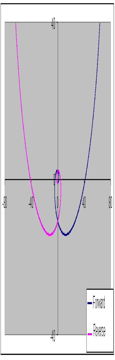
Figure 3: Classical trajectories in the complex-$x$ plane for the Hamiltonian in (1) with $\epsilon=-0.2$. These trajectories begin on the negative imaginary axis very close to the origin. One trajectory evolves forward in time and the other goes backward in time. The trajectories are open orbits and show the particle spiraling off to infinity. The trajectories begin on the principal sheet of the Riemann surface; as they cross the branch cut on the positive imaginary axis, they visit the higher and lower sheets of the surface. Note that the trajectories do not cross because they lie on different sheets.

Let us now examine closed orbits having a more complicated topological structure than the orbits shown in Fig. 2. For the rest of this section we fix $\epsilon=\pi-2$ and study the effect of varying the initial conditions. It is not difficult to find an initial condition for which the classical trajectory crosses the branch cut on the positive imaginary axis and leaves the principal sheet of the Riemann surface. In Fig. 4 we show such a trajectory. This trajectory visits three sheets of the Riemann surface, the principal sheet (sheet 0) on which the trajectory is shown as a solid line, and sheets $\pm 1$ on which the trajectory is shown as a dashed line. On the Riemann surface the resulting trajectory is $\mathcal{P}\mathcal{T}$-symmetric (left-right symmetric).

Figure 4: A classical trajectory in the complex-$x$ plane for the Hamiltonian $H=p^{2}-(ix)^{\pi}$, which is obtained by setting $\epsilon=\pi-2$ in (1). The initial condition is chosen so that the path crosses the branch cut on the positive imaginary axis and leaves the principal sheet of the Riemann surface. On the principal sheet the trajectory is indicated by a solid line. The classical particle visits two other sheets of the Riemann surface on which the trajectory is indicated by a dashed line. Note that the closed orbit is $\mathcal{P}\mathcal{T}$ symmetric (has left-right symmetry) and that the period is $T=11.8036$.

The period of the orbit in Fig. 4 is $T=11.8036$, which is roughly five times longer than the periods of the orbits shown in Fig. 2. This is because the orbit is topologically more complicated and encloses branch cuts joining three pairs rather than one pair of complex turning points. (The period of the orbit is roughly proportional to the number of times that the orbit crosses the imaginary axis.) We explain how to calculate the period of these topologically nontrivial orbits in Sec. 3.

The closed orbit shown in Fig. 4 only visits three sheets of the Riemann surface. It is possible to find initial conditions that generate trajectories that visit many sheets repeatedly. In Fig. 5 we have plotted a classical trajectory starting at $x(0)=-7.1i$. This trajectory visits 11 sheets of the Riemann surface and its period is $T=255.3$. The structure of this orbit near the origin is complicated and therefore a magnified version is shown in Fig. 6.

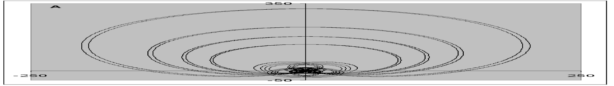
Figure 5: A classical trajectory in the complex-$x$ plane for the complex Hamiltonian $H=p^{2}-(ix)^{\pi}$. This complicated trajectory begins at $x(0)=-7.1i$ and visits 11 sheets of the Riemann surface. Its period is approximately $T=255.3$. This figure displays the projection of the trajectory onto the principal sheet of the Riemann surface. Note that this trajectory does not cross itself.

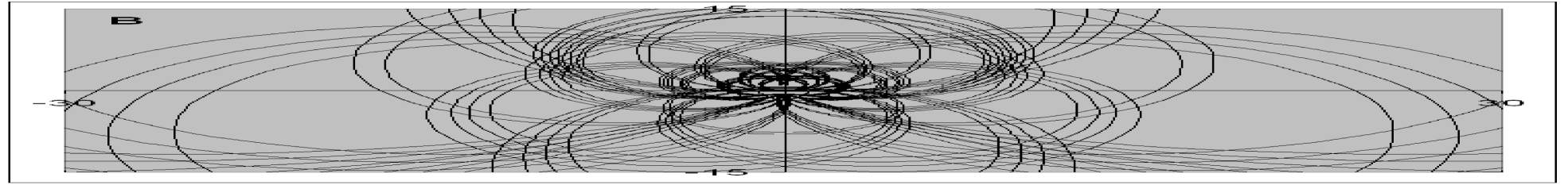
Figure 6: An enlargement of the classical trajectory $x(t)$ in Fig. 5 showing the detail near the origin in the complex-$x$ plane. We emphasize that this classical path never crosses itself; the apparent self-intersections are paths that lie on different sheets of the Riemann surface.

Because Figs. 5 and 6 are so complicated, it is useful to give a more understandable representation of the classical orbit in which we plot the complex phase (argument) of $x(t)$ as a function of $t$. In Fig. 7 we present such a plot showing the complex phase for one full period.

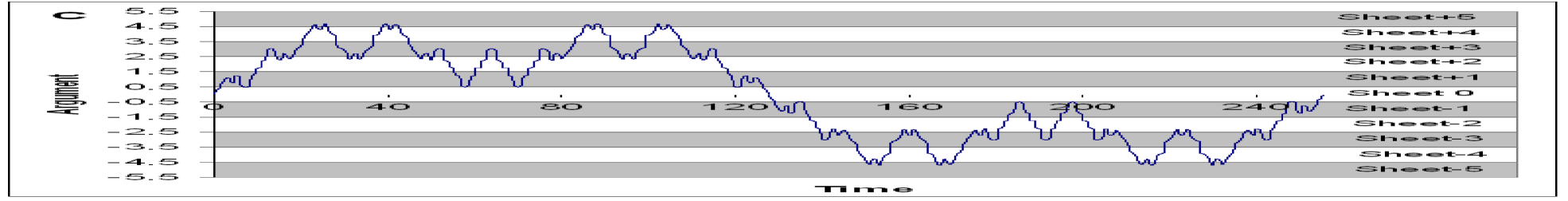
Figure 7: The argument (complex phase) of the classical orbit shown in Figs. 5 and 6 plotted as a function of time for one complete cycle. The period of this cycle is $T=255.3$. The classical particle starts on the negative imaginary axis on sheet 0 where the phase is defined to be 0. The particle then visits 11 sheets of the Riemann surface from sheet $-5$ to sheet 5.

The period of the classical orbits is exquisitely sensitive to the initial conditions. To illustrate this sensitivity we show in Fig. 8 the size of the period for $\epsilon=\pi-2$ as a function of the initial condition $x(0)$ in a small portion of the complex-$x$ plane containing the negative imaginary axis from $-8.5i$ to $-9.0i$. Note that initial conditions chosen from this small region give rise to classical orbits whose periods range from $231.1$ up to $28,104.7$. The regions of extremely long periods become narrower and more difficult to observe numerically. It is impossible to resolve the fine detail between the two longest periods, and we conjecture that there are infinitely many arbitrarily thin regions of initial conditions between $-8.767i$ and $-8.770i$ that give rise to arbitrarily long periods.

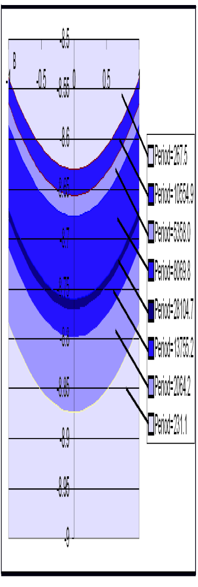
Figure 8: A small portion of the complex-$x$ plane showing the dependence of the periods $T$ of the classical orbits on the choice of initial condition $x(0)$ for the case $\epsilon=\pi-2$. Note that $T$ is extremely sensitive to the value of $x(0)$. There is an unresolved region between the band corresponding to $T=28,104.7$ and $T=13,755.2$. We conjecture that arbitrarily long periods can be found in arbitrarily thin regions between $x(0)=-8.767i$ and $x(0)=-8.770i$.

We display in Fig. 9 one of the long-period orbits taken from Fig. 8. Figure 9 shows the complex argument of $x(t)$ as a function of time $t$ for $\epsilon=\pi-2$ and initial condition $x(0)=-8.63026i$. This orbit has period $T=10,554.9$ and visits 17 sheets of the Riemann surface. The inset displays some of the fine structure of this spectacular oscillatory behavior.

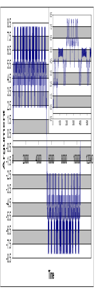
Figure 9: The argument of a long-period classical orbit for which $\epsilon=\pi-2$ and the initial condition is $x(0)=-8.63026i$. This orbit has period $T=10,554.9$ and visits 17 sheets of the Riemann surface. Note the oscillatory fine structure of this orbit in the inset.

A characteristic feature of the long orbits is the persistent oscillation in the classical path which makes huge numbers of U-turns in portions of the complex plane. These U-turns focus about one of the many complex turning points and illustrate in a rather dramatic fashion the complex nature of the classical turning point. (The behavior of real trajectories is much simpler. When a real trajectory encounters a turning point on the real axis it merely stops and reverses direction.) In Fig. 10 we plot the complex argument of $x(t)$ as a function of time $t$ for $\epsilon=\pi-2$ and initial condition $x(0)=-17i$. This orbit has period $T=452.6$ and visits 5 sheets of the Riemann surface. We show the U-turns of this orbit near a turning point in Fig. 11.

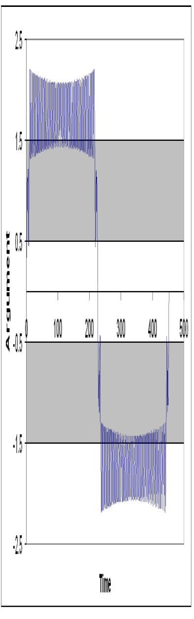
Figure 10: The argument of the classical orbit as a function of time $t$ for $\epsilon=\pi-2$ and initial condition $x(0)=-17i$. This orbit has period $T=452.6$ and visits 5 sheets of the Riemann surface. Note the persistent oscillation in the classical orbit.

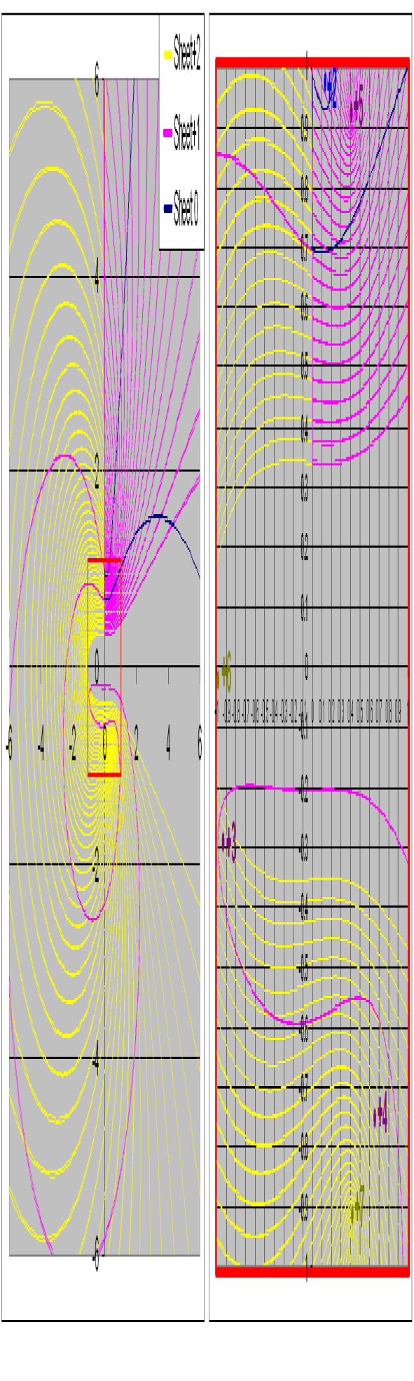
Figure 11: The classical orbit in the complex-$x$ plane corresponding to Fig. 10. The oscillation in Fig. 10 corresponds to nested U-turns around a turning point in the complex plane.

Figures 10 and 11 provide a heuristic explanation of how very long-period orbits arise. In order for a classical trajectory to travel a great distance in the complex plane, its path must weave through a mine field of turning points. If the trajectory comes under the influence of a distant turning point, it executes a huge number of nested U-turns and is eventually flung back towards its starting point. However, if the initial condition is chosen very carefully, the complex trajectory can slip past many turning points before it eventually encounters a turning point that takes control of the particle. We speculate that it may be possible to find a special critical initial condition for which the classical path manages to avoid and slip past all turning points. Such a path would have an infinitely long period.

3 Classification of classical orbits

In the previous section we explored for a fixed value of $\epsilon$ the dependence of the classical trajectories on the initial condition. By varying the initial condition (on the negative imaginary axis) we were able to produce orbits of incredible topological complexity and with extremely long periods. In this section we propose a technique for classifying these orbits. This technique relies on the observation that to calculate the period of an orbit we may use Cauchy’s integral theorem to deform and shrink the orbit into a curve that tightly encloses the square-root branch cuts that connect the $\mathcal{P}\mathcal{T}$-symmetric pairs of turning points labeled by $n$.

We will argue that all classical orbits having the same period fall into well-defined topological classes. For example, all three orbits in Fig. 2 have the same period. It is only necessary to examine the central orbits that terminate at turning points because all other orbits in the same topological class can be shrunk down to these much simpler central orbits without changing the period. This simplification allows us to classify all possible orbits merely by giving the pair of turning points at which the central orbit terminates.

The topological class of orbits shown in Fig. 2 is characterized by the central orbit connecting the $n=0$ pair of turning points. In Fig. 12 we display two classical orbits associated with the $n=1$ pair of turning points for the case $\epsilon=0.5$. In this figure we show an orbit (solid line) that encircles the turning points and a central orbit (dashed line), having the same period, that connects these turning points.

Figure 12: Two orbits for $\epsilon=0.5$ that have the same period. The solid-line orbit encircles the turning points. The dashed-line orbit is the central orbit that terminates at the $n=1$ pair of turning points. The $n=0$ and $n=1$ pairs of turning points are indicated by dots. The period of this class of orbits is $T=5.54559$.

The period of the class of orbits shown in Fig. 12 is $T=5.54559$. To calculate this number we deform the central orbit to a pair of rays that run from one turning point to the origin and then from the origin to the other turning point. However, since the turning points lie on different sheets of the Riemann surface, there are additional contributions from all other pairs of enclosed turning points. In this case the only other pair of enclosed turning points is the $n=0$ pair.

In general, there are contributions to the period integral from many enclosed pairs of turning points. We label each such pair by the integer $j$. The general formula for the period of a given topological class of classical orbits whose central orbit terminates on the $n$th pair of turning points is

$$T_{n}(\epsilon)=2\sqrt{\pi}{\Gamma\left({3+\epsilon\over 2+\epsilon}\right)\over\Gamma\left({4+\epsilon\over 4+2\epsilon}\right)}\sum_{j=0}^{\infty}a_{j}(n,\epsilon)\left|\cos\left({(2j+1)\epsilon\pi\over 4+2\epsilon}\right)\right|.$$ (6)

In this formula the cosines originate from the angular positions of the turning points in (4). The coefficients $a_{j}(n,\epsilon)$ are all nonnegative integers. The $j$th coefficient is nonzero only if the classical path encloses the $j$th pair of turning points. Each coefficient is an even integer except for the $j=n$ coefficient, which is an odd integer. The coefficients $a_{j}(n,\epsilon)$ satisfy the sum rule

$$\sum_{j=0}^{\infty}a_{j}(n,\epsilon)=K,$$ (7)

where $K$ is the number of times that the central classical path crosses the imaginary axis. This sum rule truncates the summation in (6) so that it is only a finite sum. For example, the dashed line in Fig. 12 crosses the imaginary axis three times, so that $K=3$. The formula for the period of this class of orbits has $a_{0}=2$ and $a_{1}=1$.

As we increase $\epsilon$, the topology of the classical orbits becomes more complicated. For example, when $\epsilon=1.149739$ the central orbit belonging to the $n=1$ pair of turning points crosses the imaginary axis 13 times ($K=13$). This orbit is shown in Fig. 13. For this class of orbits $a_{0}=2$, $a_{1}=1$, $a_{2}=6$, and $a_{3}=4$. The sum of these coefficients is 13.

Figure 13: Central orbit for $\epsilon=1.149739$ terminating at the $n=1$ pair of turning points. This orbit crosses the imaginary axis 13 times.

If we increase $\epsilon$ to $1.225$, the crossing number decreases to $K=9$. For this class of orbits $a_{0}=2$, $a_{1}=1$, $a_{2}=4$, and $a_{3}=2$. The central orbit for this class is shown in Fig. 14.

Figure 14: Central orbit for $\epsilon=1.225$ terminating at the $n=1$ pair of turning points. This orbit crosses the imaginary axis 9 times.

If we increase $\epsilon$ still further to $1.3$, the crossing number increases to $K=17$. For this orbit $a_{0}=2$, $a_{1}=3$, $a_{2}=8$, and $a_{3}=4$. This orbit is shown in Fig. 15.

Figure 15: Central orbit for $\epsilon=1.3$ terminating at the $n=1$ pair of turning points. This orbit crosses the imaginary axis 17 times.

For $\epsilon=2.31$ the number of crossings decreases again to $K=5$. For this orbit $a_{0}=0$, $a_{1}=3$, and $a_{2}=2$. This orbit is shown in Fig. 16. Note that unlike the orbits in Figs. 15 and 14 this orbit does not enclose the $n=0$ turning points. This is why the $a_{0}$ coefficient vanishes.

Figure 16: Central orbit for $\epsilon=2.31$ terminating at the $n=1$ pair of turning points. This orbit crosses the imaginary axis 5 times. Note that this orbit does not enclose the $n=0$ turning points.

If we continue to increase the value of $\epsilon$, the topology of the classical orbits eventually simplifies. For all $\epsilon\geq 4$ we find that $K=1$. For example, in Fig. 17 we illustrate the central orbit for $\epsilon=4.01$. For this class of orbits we have $a_{1}=1$ and all other coefficients vanish.

Figure 17: Central orbit for $\epsilon=4.01$ terminating at the $n=1$ pair of turning points. This orbit crosses the imaginary axis only once.

For small $\epsilon$ the classical orbits terminating at the $n=2$ and $n=3$ turning points behave in a similar fashion. When $\epsilon=0.2$, the $n=2$ central orbit crosses the imaginary axis 5 times and when $\epsilon=0.04$, the $n=3$ central orbit crosses the imaginary axis 7 times (see Fig. 18). In the former case $a_{0}=2$, $a_{1}=2$, and $a_{2}=1$ and in the latter case $a_{0}=2$, $a_{1}=2$, $a_{2}=2$, and $a_{3}=1$.

Figure 18: On the left the central orbit for $\epsilon=0.2$ terminating at the $n=2$ pair of turning points. This orbit crosses the imaginary axis 5 times. On the right the central orbit for $\epsilon=0.04$ terminating at the $n=3$ pair of turning points. This orbit crosses the imaginary axis 7 times.

As $\epsilon$ increases, the topology in Fig. 18 changes. For example, when $\epsilon=1.34$, the $n=2$ central orbit crosses the imaginary axis 3 times and we find that $a_{0}=2$, $a_{1}=0$, and $a_{2}=1$ (see Fig. 19).

Figure 19: Central orbit for $\epsilon=1.34$ terminating at the $n=2$ pair of turning points. This orbit crosses the imaginary axis 3 times. This orbit does not enclose the $n=1$ turning points.

We can see from Figs. 12 - 19 that a clear pattern emerges. When $\epsilon$ is small (less than $\frac{1}{n}$) the central path that joins the $n$th pair of turning points crosses the imaginary axis $K=2n+1$ times and the coefficients $a_{j}$ have a simple pattern: $a_{j}=2$ for $j<n$ and $a_{n}=1$. When $\epsilon$ is large, specifically $\epsilon>4n$, the topology of the central classical orbits becomes extremely simple and there is only one crossing ($K=1$). For this case $a_{n}=1$. The most interesting behavior occurs for intermediate values of $\epsilon$, where we observe remarkable transitions as a function of $\epsilon$ that exhibit critical behavior. This behavior is discussed in Sec. 4.

4 Critical behavior in $\epsilon$

In this section we study the behavior of the classical trajectories as the parameter $\epsilon$ is varied. We restrict our attention to the central orbits (the closed orbits that terminate at turning points).

We begin by considering the case of central orbits that terminate at the $n=1$ pair of turning ponts. For $\epsilon<1$ all orbits cross the imaginary axis three times ($K=3$). However, as $\epsilon$ approaches 1 from below, the orbits become huge and cardioid shaped, as illustrated in Fig. 20. The vertical and horizontal extent of this orbit is about $2,000$.

Figure 20: On the left the central orbit for $\epsilon=0.98$ terminating at the $n=1$ pair of turning points. This orbit crosses the imaginary axis 3 times. Note that this orbit is huge and that its shape resembles a cardioid. Our numerical studies indicate that as $\epsilon$ tends to 1, the size of the orbit becomes infinite. On the right is an enlargement showing the detail near the origin.

We have done an extremely detailed numerical study to determine the precise value of $\epsilon$ at which the size of the orbit becomes infinite. In particular, we have determined the point $y(\epsilon)$ at which the orbit crosses the negative imaginary axis. [The number $y(\epsilon)$ becomes large and negative.] We find that a very good fit to $y(\epsilon)$ when $\epsilon$ is just below 1 is given by

$$y(\epsilon)=-a(b-\epsilon)^{-\gamma}.$$ (8)

By fitting this formula to a large set of plots, we find that $b\approx 0.999947$, and we therefore assume that the exact value of $b$ is 1. The values of the other two parameters are $a\approx 0.883032$ and $\gamma\approx 1.93757$. Thus, as $\epsilon$ approaches 1 from below, we observe critical behavior characterized by the index $\gamma$. (We note that it is at $\epsilon=1$ that the angular distance between successive turning points becomes sufficiently small that the $n=1$ pair of turning points enters the principal sheet of the Riemann surface. However, we do not understand why this might cause the observed critical behavior.)

When $\epsilon$ is slightly larger than 1 it is too difficult to discern the topological structure of the orbits because these orbits are so large and complicated that they overwhelm the numerical capability of the computer. However, we can construct numerically the orbits for $\epsilon$ larger than about $1.14736$. We observe a remarkable behavior in the structure of the orbits as we approach this value of $\epsilon$ from above in the region $1.14736<\epsilon<1.169$. Specifically, when $\epsilon>1.1497389$, the $n=1$ central orbits have $K=13$ crossings as illustrated in Fig. 21 on the left. This figure shows the $K=13$ orbit for $\epsilon=1.149739$. When $\epsilon$ decreases slightly to the value $\epsilon=1.149738$ we observe a transition to an orbit with $K=25$ crossings, as shown in Fig. 21 on the right.

Figure 21: Transition between two topological classes of graphs. The left graph shows the central orbit for $\epsilon=1.149739$ terminating at the $n=1$ pair of turning points. This orbit crosses the imaginary axis 13 times. The right graph displays the central orbit for $\epsilon=1.149738$ terminating at the $n=1$ pair of turning points. This orbit crosses the imaginary axis 25 times.

As we continue to decrease $\epsilon$, we encounter a second transition from orbits having $K=25$ crossings to orbits having $K=37$ crossings. This transition occurs very near the value $\epsilon=1.14782625$. To illustrate this transition we show in Fig. 22 the $n=1$ orbits for $\epsilon=1.1478263$ (left) and for $\epsilon=1.1478262$ (right).

Figure 22: Second transition between two topological classes of graphs. The left graph shows the central orbit for $\epsilon=1.1478263$ terminating at the $n=1$ pair of turning points. This orbit crosses the imaginary axis 25 times. The right graph shows the central orbit for $\epsilon=1.1478262$ terminating at the $n=1$ pair of turning points. This orbit crosses the imaginary axis 37 times.

As $\epsilon$ continues to decrease, there is a third transition at about $\epsilon=1.14756475$ where the crossing number of the central orbits jumps from $K=37$ to $K=49$ (see Fig. 23).

Figure 23: Central orbit for $\epsilon=1.1475$ terminating at the $n=1$ pair of turning points. This orbit crosses the imaginary axis 49 times.

A fourth transition occurs at $\epsilon=1.14746085$ at which the $n=1$ orbits jump from $K=49$ crossings to $K=61$ crossings (see Fig. 24).

Figure 24: Central orbit for $\epsilon=1.14745$ terminating at the $n=1$ pair of turning points. This orbit crosses the imaginary axis 61 times.

We observe a fifth and sixth transition from $K=61$ to $K=73$ (see Fig. 25) and from $K=73$ to $K=85$ (see Fig. 26). It is clear that with each transition the value of $K$ increases by 12. The accumulation point of these transitions is close to $\epsilon=1.14736$. Throughout the region illustrated by Figs. 21 -26 there is an exact closed-form expression for the coefficients $a_{j}$ appearing in the formula (6) for the period $T$. In general, if we express the crossing number $K$ in the form $K=13+12k$ ($k=0,~{}1,~{}2,~{}\dots$), then

$$(a_{0},a_{1},a_{2},a_{3},a_{4},a_{5})=(2,1+2k,6+4k,4+4k,0,2k)$$ (9)

with all higher coefficients vanishing.

The region of $\epsilon$ between $\epsilon=1$ and $\epsilon=1.14736$ remains largely unexplored and its behavior is mysterious. We have been able to find isolated values of $\epsilon$ in this region for which we can determine the orbit numerically. (One such value is $\epsilon=1.03$, and for this value we find that $K=29$.) However, we do not understand how the topology of the orbits depends on $\epsilon$ in this region.

Figure 25: Central orbit for $\epsilon=1.1474$ terminating at the $n=1$ pair of turning points. This orbit crosses the imaginary axis 73 times.

Figure 26: Central orbit for $\epsilon=1.14737$ terminating at the $n=1$ pair of turning points. This orbit crosses the imaginary axis 85 times.

What happens to the $K=13$ orbits when $\epsilon$ increases? From a detailed numerical analysis of the classical orbits, we find a new critical point near $\epsilon=1.16898$. As $\epsilon$ approaches this critical point from below, the orbits on the principal sheet of the Riemann surface again resemble huge cardioids and the intercept on the negative imaginary axis is given by (8) with $a=0.013159$, $b=1.16898$, and the index $\gamma=1.70439$.

Beyond this value of $\epsilon$ we encounter a new and unexplored mysterious region. The upper boundary of this region is near $\epsilon=1.21$. As we approach this value of $\epsilon$ from above, we again observe a sequence of transitions in which the crossing number $K$ again appears to jump arithmetically. One orbit in this region is shown in Fig. 27 and another is shown in Fig. 14. These orbits cross the imaginary axis $K=9$ times.

Figure 27: Central orbit for $\epsilon=1.282$ terminating at the $n=1$ pair of turning points. This orbit crosses the imaginary axis 9 times. To the right is a detail of the region near the origin.

The first transition in this region of classical orbits occurs very near $\epsilon=1.21152145$. At this transition the value of the crossing number jumps from $K=9$ to $K=69$, and we observe that this change is a multiple of 12. Classical orbits just above and below this transition are shown in Fig. 28.

Figure 28: Transition between a $K=9$ orbit (left) and a $K=69$ orbit (right. The left graph shows a central $n=1$ orbit that corresponds to $\epsilon=1.2115215$ and the right graph shows a central $n=1$ orbit that corresponds to $\epsilon=1.2115214$. It is not easy to see that the right orbit actually crosses the imaginary axis 69 times, so the region of this orbit near the origin is displayed in Fig. 29.

It is very difficult to see that the orbit on the right in Fig. 28 actually crosses the imaginary axis 69 times, so in Fig. 29 we show two enlargements of the region near the origin.

Figure 29: Two enlargements of the $n=1$ central orbit for $\epsilon=1.2115214$ in Fig. 28 (right). By careful examination of these detailed graphs, one can determine that the crossing number is $K=69$.

As we continue to increase $\epsilon$, we encounter a third critical transition that marks the upper end of this region. At this transition the classical orbits on the principal sheet again resemble huge cardioids and again the intercept on the imaginary axis is well approximated by the formula (8) with $a=0.0423448$, $b=1.2837$, and the critical index $\gamma=1.55255$.

Surprisingly, we find a new kind of critical behavior above this region. For $\epsilon$ between the values $1.284$ and $1.306$ we find $n=1$ classical orbits with crossing number $K=17$. We have already shown one such orbit Fig. 15. As $\epsilon$ approaches the lower boundary of this region, the classical orbits become huge, but do not resemble cardioids. Rather, they resemble double cardioids – that is, cardioids having two notches instead of one. An example of a $K=17$ orbit near the lower edge of this region is shown in Fig. 30. As $\epsilon$ approaches the upper boundary of this region, the classical orbits once again resemble huge cardioids. An example of a $K=17$ orbit near the upper edge of this region is shown in Fig. 31.

Figure 30: Central orbit for $\epsilon=1.286$ terminating at the $n=1$ pair of turning points. This orbit crosses the imaginary axis 17 times. The central orbit is dominated by a huge double-cardioid structure having a horizontal extent of over 1000. This structure lies on the $\pm 1$ sheets of the Riemann surface. To the right is a detail of the region near the origin.

Figure 31: Central orbit for $\epsilon=1.305$ terminating at the $n=1$ pair of turning points. This orbit crosses the imaginary axis 17 times. On the principal sheet the central orbit resembles a large cardioid having a horizontal extent of over 300. To the right is a detail of the region near the origin.

The same sort of behavior characterized by narrow regions bounded by critical points is observed for orbits terminating on $n=2$ and higher critical points. Numerical studies indicate that the first critical point for $n=2$ is near $\epsilon=\frac{1}{2}$ and the first critical point for $n=3$ is approximately at $\epsilon=\frac{1}{3}$. As $\epsilon$ approaches these critical points from below, we observe the same kind of critical behavior that is expressed in (8). For the case $n=2$, we find that $a=0.071388$, $b=0.499759$, and the critical index $\gamma=3.7063$ and for the case $n=3$, we find that $a=0.008258$, $b=0.3341$, and the critical index $\gamma=5.17017$. While it is difficult to assess the precise numerical accuracy of these results, we believe that it is safe to conjecture that as a function of $n$, $b=\frac{1}{n}$. Furthermore, $a$ appears to decay geometrically with increasing $n$ and $\gamma$ seems to grow arithmetically with increasing $n$.

Eventually, this extraordinarily complicated array of regions in $\epsilon$, which are bounded by critical points, gives way to a very simple and almost featureless behavior. We find that when $\epsilon>4n$ the classical trajectories lie entirely on the principal sheet of the Riemann surface and cross the imaginary axis exactly once. We have already seen in Fig. 17 an example of this simple behavior. Four additional examples of these central classical trajectories for $\epsilon$ lying just above this transition are shown in Figs. 32 and 33. The transition to simple behavior occurs just as the $n$th pair of turning points crosses the real axis on the principal sheet of the Riemann surface.

Figure 32: On the left, central orbit terminating at the $n=2$ pair of turning points for $\epsilon=8.01$. On the right, central orbit terminating at the $n=3$ pair of turning points for $\epsilon=12.01$.

Figure 33: On the left, central orbit terminating at the $n=4$ pair of turning points for $\epsilon=16.01$. On the right, central orbit terminating at the $n=5$ pair of turning points for $\epsilon=20.01$.

While the orbits shown in Figs. 32 and 33 appear to have no interesting structure, in fact they exhibit an interesting low-amplitude oscillation. To see this oscillation we take $\epsilon$ large and plot the central curves for two values of $n$ in Fig. 34. Evidently, the number of oscillations is $2n+1$.

Figure 34: On the left, central curve terminating at the $n=5$ pair of turning points for $\epsilon=400$. On the right, central curve terminating at the $n=6$ pair of turning points for $\epsilon=400$. In general, the number of oscillations is $2n+1$.

5 Concluding remarks

This paper is a descriptive taxonomy of possible behaviors of classical trajectories of a particle that obeys the Hamiltonian (1). It is surprising how rich and elaborate these behaviors can be. We have found classical paths that are extremely sensitive to changes in initial conditions. We have also shown that the classical paths are delicately dependent on the value of $\epsilon$, so highly dependent that they exhibit critical behavior. We have also identified many problems that require further investigation, both numerical and analytic. For example, we do not understand the true nature of the multiple critical behaviors that we have discovered.

The classical behavior that we have found is in part remiscent of the period-lengthening route to chaos that is observed in logistic maps. In the case of logistic maps the critical behavior is a function of a multiplicative parameter $\lambda$, while here the parameter $\epsilon$ appears in the exponent of a complex function. It may be possible to regard the rich behavior described in this paper as a kind of complex extension of chaos theory.

References

References

- [1] C. M. Bender and S. Boettcher, Phys. Rev. Lett. 80, 5243 (1998).
- [2] P. Dorey, C. Dunning, and R. Tateo, J. Phys. A: Math. Gen. 34, L391 (2001) and 34, 5679 (2001).
- [3] C. M. Bender, D. C. Brody, and H. F. Jones, Phys. Rev. Lett. 89, 270401 (2002).
- [4] C. M. Bender, S. Boettcher, and P. N. Meisinger, J. Math. Phys. 40, 2201 (1999).
- [5] A. Nanayakkara, Czech. J. Phys. 54, 101 (2004) and J. Phys. A: Math. Gen. 37, 4321 (2004).
- [6] M. Feigenbaum, Los Alamos Science 1, 4 (1980).