Quasi-periodic Green’s functions of the Helmholtz and Laplace equations

abstract

A classical problem of free-space Green’s function $G_{0\Lambda}$ representations of the Helmholtz equation is studied in various quasi-periodic cases, i.e., when an underlying periodicity is imposed in less dimensions than is the dimension of an embedding space. Exponentially convergent series for the free-space quasi-periodic $G_{0\Lambda}$ and for the expansion coefficients $D_{L}$ of $G_{0\Lambda}$ in the basis of regular (cylindrical in two dimensions and spherical in three dimension (3D)) waves, or lattice sums, are reviewed and new results for the case of a one-dimensional (1D) periodicity in 3D are derived. From a mathematical point of view, a derivation of exponentially convergent representations for Schlömilch series of cylindrical and spherical Hankel functions of any integer order is accomplished. Exponentially convergent series for $G_{0\Lambda}$ and lattice sums $D_{L}$ hold for any value of the Bloch momentum and allow $G_{0\Lambda}$ to be efficiently evaluated also in the periodicity plane. The quasi-periodic Green’s functions of the Laplace equation are obtained from the corresponding representations of $G_{0\Lambda}$ of the Helmholtz equation by taking the limit of the wave vector magnitude going to zero. The derivation of relevant results in the case of a 1D periodicity in 3D highlights the common part which is universally applicable to any of remaining quasi-periodic cases. The results obtained can be useful for numerical solution of boundary integral equations for potential flows in fluid mechanics, remote sensing of periodic surfaces, periodic gratings, and infinite arrays of resonators coupled to a waveguide, in many contexts of simulating systems of charged particles, in molecular dynamics, for the description of quasi-periodic arrays of point interactions in quantum mechanics, and in various ab-initio first-principle multiple-scattering theories for the analysis of diffraction of classical and quantum waves.

PACS numbers: 02.70.Pt; 03.65.Db; 03.65.Nk; 34.20.-b; 42.25.Fx; 46.40.Cd; 47.15.km; 61.14.Hg

1 Introduction

Let $\Lambda$ be a $d_{\Lambda}$-dimensional simple (Bravais) periodic lattice embedded in a space of dimension $d\geq d_{\Lambda}$ (the condition of a simple lattice can easily be relaxed to an arbitrary periodic lattice by following recipes of Refs. [2, 3, 4, 5, 6]). Let ${\cal H}_{0}^{+}$ stand for the cylindrical ($H_{0}^{(1)}$) and spherical ($h_{0}^{(1)}$) Hankel functions in $d=2$ and $d=3$, respectively, ${\cal Y}_{L}$ be corresponding angular momentum harmonics (cylindrical in $d=2$ and spherical in $d=3$; see also Appendix B) for properties of ${\cal Y}_{L}$), and ${\bf r}$ and ${\bf r}^{\prime}$ be spatial points. The article is concerned with an efficient calculation of the series

$$\sum_{{\bf r}_{n}\in\Lambda}{\cal H}_{l}^{+}(\sigma|{\bf r}-{\bf r}^{\prime}+{\bf r}_{n}|){\cal Y}_{L}^{*}(\hat{{\bf r}}_{n})e^{i{\bf k}\cdot{\bf r}_{n}},$$ (1)

where the origin of coordinates is in the lattice, ${\bf k}$ is called the Bloch momentum, $\sigma=2\pi/\lambda$ denotes a wave vector magnitude ($\sigma$ is not necessarily equal to $|{\bf k}|$), $\lambda$ is a wavelength, and $L$ is, in general, a multi-index of angular momentum numbers [e.g., $L=(lm)$ in three dimensions with $l\geq 0$ and $-l\leq m\leq l$].

In mathematical literature such a series are known as Schlömilch series [7, 8, 9]. As first noted by Emersleben [10], in three dimensions (3D) in the special case of ${\bf r}-{\bf r}^{\prime}=0$ and $l=\sigma=0$ the series reduce to Epstein zeta functions [11, 12, 13]. A physical motivation to investigate such a series derives from a fact that, for $l=0$, the series (1) are prerequisite to determine a corresponding free-space (quasi-) periodic Green’s function $G_{0\Lambda}$ of a scalar Helmholtz equation (see below). For $l\neq 0$ and ${\bf r}-{\bf r}^{\prime}=0$, with singular term being excluded, the series (1) then formally determine the lattice sums $D_{L}$, which are defined as the expansion coefficients $G_{0\Lambda}$ in the basis of cylindrical and spherical Bessel functions in 2D and 3D, respectively [see Eqs. (8), (11) below].

However, analytic closed expressions for such series are only known for $l=0$ in two particular cases in 3D: (i) in the case of a one-dimensional (1D) periodicity [14, 15, 16] and, when additionally $\sigma=0$ (the Laplace limit), (ii) for a two-dimensional (2D) periodicity [15]. Otherwise the summation in (1) has to be performed numerically. However, since

$${\cal H}_{l}^{+}(z)\sim c_{h}z^{-(d-1)/2}\left(\frac{2}{\pi}\right)^{(d-1)/2}\exp\left\{i\left[z-(d-1)\pi/4-l\pi/2\right]\right\}$$ (2)

as $z\rightarrow\infty$ and $-\pi<\arg{z}<2\pi$, where $c_{h}=1$ unless $d=2$, in which case $c_{h}=\sqrt{2/\pi}$ (see Eqs. (9.2.3) and (10.1.1) of Ref. [17]), the series (1) is not absolutely convergent. Even if one assumes that $\sigma$ has an infinitesimally small positive imaginary part, and thereby establishing absolute convergence, the convergence of the series in Eq. (1) is notoriously slow, thereby rendering it useless for practical applications.

The study of efficient techniques for the calculation of $G_{0\Lambda}$ and lattice sums $D_{L}$ has a long history [2, 3, 5, 9, 18, 19, 20, 21, 22, 23, 24, 25] and the topic has roots and branches in widely differing areas of chemistry, physics, and mathematics. Despite that it still continues to be a perennial research subject [6, 26, 27, 28, 29, 30, 31, 32, 33, 34, 35, 36, 37, 38]. However, quite often this happens merely because researches in widely differing areas of chemistry, physics, and mathematics are not aware of the techniques and results developed in connection with the so-called Korringa-Kohn-Rostoker (KKR) [2, 3, 24, 25] and layer Korringa-Kohn-Rostoker (LKKR) theories either for quantum (electron) waves within low-energy electron diffraction (LEED) theory [5, 21, 22, 23] or for various classical (acoustic, elastic, electromagnetic, water) waves [6, 27, 28]. Therein exponentially convergent series for $G_{0\Lambda}$ and lattice sums $D_{L}$ have been derived for a number of cases. In a periodic case ($d_{\Lambda}=d$), efficient computational schemes for $G_{0\Lambda}$ and lattice sums $D_{L}$ have been provided more than thirty years ago [3, 24]. The quasi-periodic case $d_{\Lambda}=2$ and $d=3$ has been investigated in detail in a series of articles by Kambe almost forty years ago [5, 21, 22]. The case $d_{\Lambda}=1$ and $d=2$ has been dealt with only relatively recently in Refs. [6, 27]. Surprisingly enough, the case $d_{\Lambda}=1$ and $d=3$ has not been studied in full detail yet, although it may provide an efficient description of “wave integrated circuits”.

Therefore, in the following we shall focus on the so-called quasi-periodic, or layer, case, when the underlying lattice $\Lambda$ is of lower dimensionality than the embedding space ($d_{\Lambda}<d$), and, in particular, on the $d_{\Lambda}=1,\,d=3$ case. There are many physical problem which would profit from an efficient computational scheme for $G_{0\Lambda}$ and lattice sums $D_{L}$ in the case of 1D periodicity in 3D. For instance, a Green’s function representing a point source and satisfying the respective von Neumann and Dirichlet boundary condition on a flow channel walls in fluid mechanics for the flow between parallel planes can be written as a sum and difference of $G_{0\Lambda}$ corresponding to 1D periodicity in 3D taken at two different spatial points [31]. (For the flow in a rectangular channel, the relevant $G_{0\Lambda}$ would then correspond to 2D periodicity in 3D [31].) Another problem involves infinite arrays of resonators coupled to a waveguide which by itself may have a plethora of photonics applications [39]. Moreover, recent progress in nanotechnology made it possible to fabricate 1D chains of metal nanoparticles [40, 41] and dielectric microparticles [42]. Additionally, understanding of linear periodic arrays of lossless spheres is germane for the qualitative description of a finite-lengths periodic arrays of small antennas [43]. In a linear chain of spherical metal nanoparticles light can be transmitted by electrodynamic interparticle coupling resulting in a subwavelength-sized light guide [40, 41, 44, 45, 46]. So far, infinite 1D linear chains of particles have only been investigated within the one particle theory framework of Schrödinger equation for the description of polymers [16], in the electrostatic limit within the framework of the Laplace equation [45], or in the dipole approximation [43, 46, 47]. Moreover, the energy operator in the one-particle theory of periodic point (zero-range) interactions is constructed in terms of an auxiliary operator which corresponds essentially to the operator of multiplication by $D_{00}$ ($\gamma$ function of Karpeshina [14, 48]).

In the following, exponentially convergent series for the free-space quasi-periodic $G_{0\Lambda}$ and for the lattice sums $D_{L}$ are reviewed and new results for the case of a 1D periodicity in 3D are derived [see Eqs. (LABEL:dl1f1in3), (98), and (109) below]. The derivation of relevant results for the case of a 1D periodicity in 3D is performed in such a way that the common part which is universally applicable to any of the remaining quasi-periodic cases is highlighted. Thereby a link with earlier results by Kambe [5, 21] for a 2D periodicity in 3D can easily be established and the proof of results for a 1D periodicity in 2D announced in Ref. [27] can easily be carried out.

1.1 The outline of the article

The article is organized as follows. Sec. 2 introduces notation, provides some necessary definitions and gives an overview of some of the problems requiring the knowledge $G_{0\Lambda}$ and lattice sums. In Sec. 3, $G_{0\Lambda}$ is expressed as an exponentially convergent sum over a dual lattice $\Lambda^{*}$. Such a dual representation of $G_{0\Lambda}$ is then a starting point in the derivation of a corresponding exponentially convergent Ewald representation of $G_{0\Lambda}$ in Sec. 4. As in the bulk case, a derivation of the Ewald representation invokes a suitable integral representation of Hankel functions and a Jacobi identity (see Appendix D below). In addition, following Kambe [22], an analytic continuation procedure is employed, which is analogous to finding the values of the Riemann $\zeta$-function outside the domain of absolute convergence of a defining series (see Ref. [49], p. 273). The Ewald representation of $G_{0\Lambda}$, which is a hybrid sum over both $\Lambda$ and dual lattice $\Lambda^{*}$, converges uniformly and absolutely over bounded sets of ${\bf R}$. Unlike the dual representation, the Ewald representation can also be efficiently evaluated in the periodicity plane (provided that it remains ${\bf R}\not\in\Lambda$).

Exponentially convergent series for the lattice sums $D_{L}$ in the case of a 1D periodicity in 3D are derived in Sec. 5. Eqs. (LABEL:dl1f1in3), (98), (109) of the section are the main new results of this paper.

In Sec. 6 the quasi-periodic Green’s function of the Laplace equation are obtained from that of the Helmholtz equation by taking the limit $\sigma\rightarrow 0$. We then end up with discussion (Sec. 7) and summary and conclusions (Sec. 8).

To make this paper as readable as possible, several technical arguments have been relegated to a number of appendices. Appendix A summarizes relevant integral representations of ${\cal H}^{+}_{l}$ and Appendix B lists relevant properties of harmonics ${\cal Y}_{L}$. Some useful properties of free-space scattering Green’s function are collected in Appendix C, whereas Appendix D shows several forms of Jacobi identities. In Appendix E the dual representation of the quasi-periodic Green’s functions is derived by following original path of McRae [50] for a 2D periodicity in 3D, i.e., by applying an Ewald integral representation and the generalized Jacobi identity. Some of the general properties of free-space quasi-periodic Greens functions and the lattice sums are outlined in Appendix F. Alternative definitions of lattice sums and structure constants are then summarized in Appendix G.

2 Notation and definitions: $G_{0\Lambda}$ and lattice sums

2.1 $G_{0\Lambda}$

A corresponding free-space (quasi-) periodic Green’s function $G_{0\Lambda}$ of a scalar Helmholtz equation is defined by an image-like series

$$G_{0\Lambda}(\sigma,{\bf k},{\bf R})=\sum_{{\bf r}_{n}\in\Lambda}G_{0}^{+}(\sigma,{\bf R}+{\bf r}_{n})e^{-i{\bf k}\cdot{\bf r}_{n}}=\sum_{{\bf r}_{n}\in\Lambda}G_{0}^{+}(\sigma,{\bf R}-{\bf r}_{n})e^{i{\bf k}\cdot{\bf r}_{n}},$$ (3)

where the origin of coordinates is in the lattice. Here $G_{0}^{+}$ is the free-space scattering, or retarded, Green’s function of a scalar Helmholtz equation in $d$ dimensions,

$$\left[\Delta+\sigma^{2}\right]G_{0}(\sigma,{\bf r},{\bf r}^{\prime})=\delta({\bf r}-{\bf r}^{\prime}),$$ (4)

$\Delta$ being a corresponding Laplace operator, which is represented for large $R=|{\bf R}|=|{\bf r}-{\bf r}^{\prime}|$ by outgoing waves (i.e. satisfies Sommerfeld radiation condition). Since $G_{0}^{+}$ is only a function of ${\bf R}={\bf r}-{\bf r}^{\prime}$, the functional dependence of $G_{0}^{+}$ has been written as $G_{0}^{+}(\sigma,{\bf R})$ in Eq. (3).

$G_{0}^{+}$ is proportional to an appropriate Hankel function of zero order [17]

$$G_{0}^{+}(\sigma,{\bf R})=\lim_{\epsilon\rightarrow 0_{+}}\frac{1}{(2\pi)^{d}}\int\frac{e^{i{\bf k}\cdot{\bf R}}}{\sigma^{2}-k^{2}+i\epsilon}\,d{\bf k}=-i\frac{\pi}{2}\,\frac{A}{(2\pi)^{d}}\,\sigma^{d-2}{\cal H}_{0}^{+}(\sigma R)$$ (5)

(see also Appendix C). Here $k=|{\bf k}|$ and $A$ is the surface of a unit sphere in $d$-dimensions [see Eq. (136) below]. (With ${\cal H}_{0}(z)=e^{iz}$ as a one-dimensional (1D) analog of the Hankel function [51] Eq. (5) becomes also valid for $d=1$, in which case $A=2$ (unit “sphere” in 1D consists of two points).) Consequently, upon substituting (5) into (3) one arrives up to a proportionality factor to the special case of series (1) for $l=0$.

A scalar Helmholtz equation is employed for the description of various waves arising in acoustics, mechanics, fluid dynamics, electromagnetism, and quantum mechanics [52]. An important class of problems which requires an efficient calculation of $G_{0\Lambda}$ arises in connection with remote sensing of periodic surfaces [26], numerical solution of boundary integral equations for potential flows in fluid mechanics [29, 30, 31, 32], periodic gratings, and infinite arrays of resonators coupled to a waveguide [39], in descriptions of dipolar fields in simulated liquid-vapour interfaces [53], in many contexts of simulating systems of charged particles, such as crystal binding and lattice vibrations [10, 12], Madelung constant [12, 13], in various problems in molecular dynamics and Monte Carlo simulations of particles interacting by long-range Coulomb forces [33, 54], wherein periodic boundary conditions are usually imposed in order to avoid the boundary effects.

2.2 Lattice sums

Within a primitive cell of $\Lambda$, the respective Green’s functions $G_{0}^{+}$ and $G_{0\Lambda}$ only differ up to boundary conditions and their respective singular parts are identical. For the scalar Helmholtz equation, the singular, or principal-value, part of $G_{0}^{+}$ is

$$G_{0}^{p}(\sigma,{\bf R})=\mbox{Re}\,G_{0}^{+}(\sigma,{\bf R})=\left\{\begin{array}[]{cc}N_{0}(\sigma R)/4,&2D\\ -\cos(\sigma R)/(4\pi R),&3D\end{array}\right.$$ (6)

where $N_{0}$ is the cylindrical Neumann function [17]. Therefore, the difference

$$D_{\Lambda}(\sigma,{\bf k},{\bf R})=G_{0\Lambda}(\sigma,{\bf k},{\bf R})-G_{0}^{p}(\sigma,{\bf R})$$ (7)

is regular for ${\bf R}\rightarrow 0$ and can be expanded in terms of regular [cylindrical in 2D, spherical in 3D] waves [3, 5, 21, 24, 27, 28, 55]

$$D_{\Lambda}(\sigma,{\bf k},{\bf R})=\sum_{L}D_{L}(\sigma,{\bf k}){\cal J}_{l}(\sigma R){\cal Y}_{L}(\hat{{\bf R}}).$$ (8)

Here the symbol ${\cal J}_{l}$ stands for cylindrical and spherical Bessel functions in 2D and 3D, respectively. The expansion coefficients $D_{L}(\sigma,{\bf k})$ introduced by Eq. (8) are then the sought lattice sums. The choice of what to subtract off in Eq. (7) is somewhat arbitrary and other choices will lead to slight amended expressions for the lattice sums $D_{L}$ (see also Appendix G). The present choice goes back to Kohn and Rostoker [55] and has been adopted by Ham and Segall [3], Kambe [5, 21], Pendry [23], and others [27, 28].

The series (1) for $l\neq 0$ then formally determine the lattice sums $D_{L}$. Indeed, the free space Green’s function is known to possess a partial wave expansion,

$$G_{0}^{+}(\sigma,{\bf r},{\bf r}^{\prime})=-iAC\sum_{L}{\cal J}_{l}(\sigma r_{<}){\cal H}_{l}^{+}(\sigma r_{>}){\cal Y}_{L}(\hat{{\bf r}}_{<}){\cal Y}_{L}^{*}(\hat{{\bf r}}_{>}),$$ (9)

where $r_{>}$ ($r_{<}$) is the larger (smaller) of the $|{\bf r}|$ and $|{\bf r}^{\prime}|$. The numerical constant C [see Eq. (10) or Eq. (137) below] is basically the prefactor in Eq. (5). Note that

$$AC=\frac{\pi}{2}\,\frac{A^{2}}{(2\pi)^{d}}\,\sigma^{d-2}=\left\{\begin{array}[]{ll}\frac{1}{\sigma},&1D\\ \frac{\pi}{2},&2D\\ \sigma,&3D.\end{array}\right.$$ (10)

When the partial wave expansion is substituted for $G_{0}^{+}$ in the series (3) for $G_{0\Lambda}$, then, according to Eqs. (7), (8), one has

$$D_{L}(\sigma,{\bf k})=-iCA^{1/2}\delta_{L0}-iAC\sum_{{\bf r}_{n}\in\Lambda}{}^{{}^{\prime}}{\cal H}_{l}^{+}(\sigma r_{n}){\cal Y}_{L}^{*}(\hat{{\bf r}}_{n})e^{i{\bf k}\cdot{\bf r}_{n}},$$ (11)

where a prime on summation sign will here and hereafter indicate that the term ${\bf r}_{n}=0$ is omitted from the sum. Note that the series is, up to a constant term and a proportionality factor, the special case of series (1) for $l\neq 0$ and ${\bf R}=0$.

It is worthwhile to point out that one is often rather interested in the lattice sums $D_{L}$ than at $G_{0\Lambda}$ itself. For instance, since $D_{L}{}$’s do not depend on ${\bf R}$, $G_{0\Lambda}$ can be evaluated using Eqs. (7) and (8) at any observation point with the same set of the lattice sums. This can in turn significantly speed-up numerical solutions of various boundary-value problems. Knowledge of the lattice sums $D_{L}$ is a key to efficient numerical analysis of various ab-initio first-principle multiple-scattering problems, such as band structure calculation within Korringa-Kohn-Rostoker (KKR) theories [2, 3, 55, 24, 56, 57, 58, 59, 60, 61, 62, 63, 64, 65, 66], and diffraction problems by periodic structures, or gratings, using the so-called layer KKR (LKKR) theories or equivalents thereof, either for quantum (electron) waves within low-energy electron diffraction (LEED) theory [5, 21, 23, 67, 68] or, for various classical (acoustic, elastic, electromagnetic, water) waves [6, 27, 66, 69, 70, 71, 72, 73, 74, 75]. Lattice sums also arise in quantizing classically ergodic systems such as Sinai’s billiard [25] and its various electromagnetic analogs [25, 76]. Moreover, the spectrum within the one-particle theory of periodic point (zero-range) interactions is determined as the set of those $z$ which, for a given ${\bf k}_{\parallel}$ and $\alpha$, satisfy an implicit equation [14, 48]

$$D_{00}(i\sqrt{-z},{\bf k}_{\parallel})=\tilde{\alpha}.$$ (12)

The spectral parameter $\tilde{\alpha}$ here is a boundary-condition parameter which determines the asymptotic of eigenfunctions at the lattice points and is the same for all the eigenfunctions [14, 48, 77].

3 Dual representations of quasi-periodic $G_{0\Lambda}$

Let $\Lambda^{*}$ be a corresponding dual (momentum) lattice, i.e., for any ${\bf r}_{n}\in\Lambda$ and ${\bf k}_{s}\in\Lambda^{*}$ one has ${\bf r}_{n}\cdot{\bf k}_{s}=2\pi N$, where $N$ is an integer. It is well known that $G_{0\Lambda}$ has an alternative representation as a sum over the dual lattice $\Lambda^{*}$. For example, in the bulk case, i.e., when $d_{\Lambda}=d$, the dual sum representation of $G_{0\Lambda}$ is

$$G_{0\Lambda}(\sigma,{\bf k},{\bf R})=\frac{1}{v_{0}}\sum_{{\bf k}_{s}\in\Lambda^{*}}\frac{e^{i({\bf k}+{\bf k}_{s})\cdot{\bf R}}}{\sigma^{2}-({\bf k}+{\bf k}_{s})^{2}}=\sum_{{\bf k}_{s}\in\Lambda^{*}}\frac{\psi({\bf k}+{\bf k}_{s},{\bf r})\overline{\psi}({\bf k}+{\bf k}_{s},{\bf r}^{\prime})}{\sigma^{2}-({\bf k}+{\bf k}_{s})^{2}},$$ (13)

with eigenfunctions

$$\psi({\bf k}+{\bf k}_{s},{\bf r})=\frac{1}{\sqrt{v_{0}}}\,e^{i({\bf k}+{\bf k}_{s})\cdot{\bf r}}$$ (14)

normalized to unity in the fundamental (Wigner-Seitz) domain,

$$\int_{WS}\bar{\psi}({\bf k}+{\bf k}_{s},{\bf r})\overline{\psi}_{(}{\bf k}+{\bf k}_{s^{\prime}},{\bf r})\,d{\bf r}=\delta_{ss^{\prime}},$$ (15)

$v_{0}$ being the volume of a unit-cell of $\Lambda$. A dual representation is sometime called an eigenfunction expansion of $G_{0\Lambda}$. Often the respective representations (3) and (13) of $G_{0\Lambda}$ are also called the spatial-domain and spectral-domain forms, respectively [29, 30, 32, 34, 36]).

In the following, the dual sum representation of $G_{0\Lambda}$ in the quasi-periodic case of 1D periodicity in 3D will be derived and its convergence properties will be discussed. However, before proceeding any further, it turns out expedient to provide some supplementary geometrical definitions which are up to minor variations adopted, for instance, within LEED and LKKR theories [5, 21, 23, 27, 28, 67, 68, 69, 70, 71, 73, 74, 75].

3.1 Supplementary geometrical definitions

In the quasi-periodic case we define the respective parallel and perpendicular components ${\bf r}_{\parallel}$ and ${\bf r}_{\perp}$ of a given vector ${\bf r}={\bf r}_{\parallel}+{\bf r}_{\perp}$ with respect to the $d_{\Lambda}$-dimensional plane containing the Bravais lattice $\Lambda$ (i.e., line for $d_{\Lambda}=1$ and surface for $d_{\Lambda}=2$) and its normal ${\bf n}$ , respectively. Then for any ${\bf r}_{n}\in\Lambda$,

$${\bf r}\cdot{\bf r}_{n}={\bf r}_{\parallel}\cdot{\bf r}_{n},\hskip 42.67912pt{\bf r}_{\perp}\cdot{\bf r}_{n}\equiv 0.$$

The respective projections ${\bf k}_{\parallel}$ and ${\bf k}_{\perp}$ of wave vector ${\bf k}={\bf k}_{\parallel}+{\bf k}_{\perp}$ are then defined in like manner with respect to $\Lambda^{*}$. Obviously, in a quasi-periodic case the quantities $G_{0\Lambda}(\sigma,{\bf k},{\bf R})$, $D_{\Lambda}(\sigma,{\bf k},{\bf R})$ and $D_{L}(\sigma,{\bf k})$ entering Eqs. (3), (7), (8), (11) are only functions of ${\bf k}_{\parallel}$. Therefore, in the quasi-periodic case, i.e., if the underlying lattice $\Lambda$ is of lower dimensionality than the embedding space ($d_{\Lambda}<d$), it is more appropriate to call merely the projection ${\bf k}_{\parallel}$ as the Bloch momentum.

A plane wave $e^{i{\bf k}\cdot{\bf r}}$ incident on a scattering plane of identical scatterers arranged regularly on $\Lambda$ would (see Fig. 1), in general, be diffracted (transmitted) to a wave with a wave vector ${\bf K}_{n}^{-}$ (${\bf K}_{n}^{+}$), where ${\bf K}_{n}^{\pm}=\left({\bf k}_{\parallel}+{\bf k}_{n},K_{\perp n}^{\pm}\right)$,

$$K_{\perp n}^{\pm}=\pm K_{\perp n}=\left\{\begin{array}[]{cc}\pm[\sigma^{2}-|{\bf k}_{\parallel}+{\bf k}_{n}|^{2}]^{1/2},&\sigma^{2}\geq|{\bf k}_{\parallel}+{\bf k}_{n}|^{2}\\ \pm i[|{\bf k}_{\parallel}+{\bf k}_{n}|^{2}-\sigma^{2}]^{1/2},&\sigma^{2}<|{\bf k}_{\parallel}+{\bf k}_{n}|^{2},\end{array}\right.$$ (16)

${\bf k}_{n}\in\Lambda^{*}$, and $|{\bf k}|=|{\bf K}_{n}^{\pm}|=\sigma$. Here $K_{\perp n}$ is indicated as a scalar, which is definitely true for $d-d_{\Lambda}=1$. In the case of a 1D periodic chain in 3D ($d-d_{\Lambda}=2$) $K_{\perp n}$ will be taken as the projection of ${\bf K}_{\perp n}$ on the plane spanned by the wave vectors of incident and diffracted beams. In the above definition, the projection ${\bf K}_{\parallel n}={\bf k}_{\parallel}+{\bf k}_{n}$ is real but the normal projection $K_{\perp n}$ can be either real or imaginary. In the case of real $K_{\perp n}$ we speak of a propagating wave, and in the case of imaginary $K_{\perp n}$ of an evanescent wave.

In the present case the scatterers are absent. Nevertheless, it turns out expedient to define wave vectors ${\bf K}_{n}^{\pm}$ and the respective projections ${\bf K}_{\parallel n}$ and $K_{\perp n}^{\pm}$ even in the free-space case.

3.2 Resulting series

In order to establish a dual representation of a quasi-periodic $G_{0\Lambda}$ for $d-d_{\Lambda}=2$, i.e. a 1D periodicity along the $x$-axis in 3D, one first substitutes the integral representation (5) of $G_{0}^{+}$ into defining equation (3) of a free-space quasi-periodic Green’s function $G_{0\Lambda}$. Then the Poisson formula

$$\sum_{{\bf r}_{n}\in\Lambda}e^{i({\bf q}_{\parallel}-{\bf k}_{\parallel})\cdot{\bf r}_{\parallel n}}=\frac{(2\pi)^{d_{\Lambda}}}{v_{0}}\sum_{{\bf k}_{n}\in\Lambda^{*}}\delta({\bf q}_{\parallel}-{\bf k}_{\parallel}-{\bf k}_{n})$$ (17)

is applied resulting in

$$G_{0\Lambda}(\sigma,{\bf k}_{\parallel},{\bf R})=\frac{(2\pi)^{d_{\Lambda}-d}}{v_{0}}\sum_{{\bf k}_{n}\in\Lambda^{*}}\int\frac{e^{i{\bf q}_{\perp}\cdot{\bf R}_{\perp}+i({\bf k}_{\parallel}+{\bf k}_{n})\cdot{\bf R}_{\parallel}}}{\sigma^{2}-{\bf q}_{\perp}^{2}-|{\bf k}_{\parallel}+{\bf k}_{n}|^{2}+i\epsilon}\,d{\bf q}_{\perp}.$$ (18)

Now the 2D plane-wave expansion (135) is applied to $e^{i{\bf q}_{\perp}\cdot{\bf R}_{\perp}}$. Using the orthonormality of cylindrical harmonics $Y_{l}=e^{il\phi}/\sqrt{2\pi}$ one finds [Eq. (134)]

$$\int_{0}^{2\pi}Y_{l}(\phi)\,d\phi=\sqrt{2\pi}\,\delta_{l0}.$$

Therefore, integration in the integral representation (18) of $G_{0\Lambda}$ over ${\bf q}_{\perp}$ results in

$$G_{0\Lambda}(\sigma,{\bf k}_{\parallel},{\bf R}) = \frac{(2\pi)^{d_{\Lambda}-d+1}}{v_{0}}\sum_{{\bf k}_{n}\in\Lambda^{*}}e^{i({\bf k}_{\parallel}+{\bf k}_{n})\cdot{\bf R}_{\parallel}}\int_{0}^{\infty}\frac{q_{\perp}J_{0}(q_{\perp}|R_{\perp}|)}{\sigma^{2}-q_{\perp}^{2}-|{\bf k}_{\parallel}+{\bf k}_{n}|^{2}+i\epsilon}\,dq_{\perp}$$ (19)

$$= -\frac{i}{4v_{0}}\sum_{{\bf k}_{n}\in\Lambda^{*}}e^{i({\bf k}_{\parallel}+{\bf k}_{n})\cdot{\bf R}_{\parallel}}H_{0}(K_{\perp n}|R_{\perp}|).$$

Here in going from the first to second equality the integral identity (138) for 2D case has been applied. Thereby the sum over ${\bf r}_{n}\in\Lambda$ has been transformed into a sum over ${\bf k}_{n}\in\Lambda^{*}$ resulting in the so-called dual representation (spectral domain form) of $G_{0\Lambda}$.

3.2.1 Complementary cases

For completeness, in the case of codimension one ($d-d_{\Lambda}=1$), one first performs a partial integral over ${\bf R}_{\perp}$ in the integral representation (5) of free-space Green’s function. This amounts to picking up a residue of a contour integral in the complex plane according to Cauchy theorem resulting in

$$G_{0}^{+}(\sigma,{\bf R})=-\frac{\pi i}{(2\pi)^{d}}\int\frac{e^{i{\bf q}_{\parallel}\cdot{\bf R}_{\parallel}+i\sqrt{\sigma^{2}-{\bf q}_{\parallel}^{2}}|R_{\perp}|}}{\sqrt{\sigma^{2}-{\bf q}_{\parallel}^{2}}}\,d{\bf q}_{\parallel}.$$ (20)

Substituting the integral representation of $G_{0}^{+}(\sigma,{\bf R})$ into defining equation (3) of a free-space quasi-periodic Green’s function $G_{0\Lambda}$ then results in

$$G_{0\Lambda}(\sigma,{\bf k}_{\parallel},{\bf R}) = -\frac{\pi i}{(2\pi)^{d}}\int\frac{e^{i{\bf q}_{\parallel}\cdot{\bf R}_{\parallel}+i\sqrt{\sigma^{2}-{\bf q}_{\parallel}^{2}}|R_{\perp}|}}{\sqrt{\sigma^{2}-{\bf q}_{\parallel}^{2}}}\,\left[\sum_{{\bf r}_{n}\in\Lambda}e^{i({\bf q}_{\parallel}-{\bf k}_{\parallel})\cdot{\bf r}_{\parallel n}}\right]\,d{\bf q}_{\parallel}$$ (21)

$$= -\frac{i}{2v_{0}}\sum_{{\bf k}_{n}\in\Lambda^{*}}\frac{e^{i({\bf k}_{\parallel}+{\bf k}_{n})\cdot{\bf R}_{\parallel}+iK_{\perp n}|R_{\perp}|}}{K_{\perp n}}$$

$$= \frac{|R_{\perp}|}{2v_{0}}\sum_{{\bf k}_{n}\in\Lambda^{*}}e^{i({\bf k}_{\parallel}+{\bf k}_{n})\cdot{\bf R}_{\parallel}}\,h_{0}^{(1)}(K_{\perp n}|R_{\perp}|).$$

where $K_{\perp n}$ is given by Eq. (16). Here in going from the first to second equality the Poisson formula (17) has been applied. Note in passing that the respective dual representations for a 1D periodicity in 2D and 2D periodicity in 3D are formally identical, the only difference being the dimensionality of $\Lambda^{*}$ in (21).

Since exponentials in the second equality in (21) can be rewritten as a product of two “eigenfunctions”, the dual representation can be recast in the form of an eigenfunction expansion of $G_{0\Lambda}$ [cf. Eq. (13)]. On the other hand, since $H_{0}(K_{\perp n}|R_{\perp}|)$ in Eq. (19) cannot be factored out as a product of two “eigenfuctions”, an eigenfunction interpretation of a dual representation is obscured for the case of a 1D periodicity in 3D.

3.3 Convergence and limiting cases

Note that, according to Eq. (16), $K_{\perp n}$ is purely imaginary with positive imaginary part for $|{\bf k}_{\parallel}+{\bf k}_{n}|>\sigma$. For purely imaginary argument $z=ix$ with $x>0$ the Hankel functions $H_{0}^{(1)}(ix)$ are related to modified Bessel functions $K_{0}(x)$ (Eq. (9.6.4) of Ref. [17]), whereas $h_{0}^{(1)}(ix)$ in the series for $d-d_{\Lambda}=2$ are related to modified Bessel functions of third kind $\sqrt{\pi/(2x)}K_{1/2}(x)$ (Eq. (10.2.15) of Ref. [17]). This results in rapidly decaying terms and exponential convergence (see Eqs. (9.7.2) and (10.2.17) of Ref. [17]). Exponential convergence can also be directly inferred from the explicit expression for

$$h_{0}^{(1)}(z)=\frac{e^{iz}}{iz}\cdot$$ (22)

One then easily finds that the respective terms in series (21) become exponentially decreasing with increasing $|{\bf k}_{\parallel}+{\bf k}_{n}|$ for $R_{\perp}\neq 0$. Since $H_{0}^{(1)}(z)\sim\sqrt{2/(\pi z)}\,e^{i(z-\pi/4)}$ for $|z|\rightarrow\infty$ and $-\pi<\mbox{arg}\,z<2\pi$ (see Eq. (9.2.3) of Ref. [17]; see also Eq. (2) above), similar applies to the series (19). Therefore, although the convergence of a dual representation of Green’s function is initially (for $|{\bf k}_{\parallel}+{\bf k}_{n}|\leq\sigma$) slow as the series consists of mere oscillating terms, afterward (for $|{\bf k}_{\parallel}+{\bf k}_{n}|>\sigma$) convergence becomes exponential for $R_{\perp}\neq 0$ (assuming as usual $K_{\perp n}\neq 0$).

Note in passing that all the dual representations of the reduced sums are nonanalytic in $R_{\perp}$ as they are functions of $|R_{\perp}|$. In the case of series (21) one has

$$|R_{\perp}|h_{0}^{(1)}(K_{\perp n}|R_{\perp}|)\rightarrow-i/K_{\perp n}\hskip 42.67912pt\mbox{as }|R_{\perp}|\rightarrow 0.$$

Therefore, absolute convergence of the resulting series in the limiting case cannot be established even for a 1D periodicity in 2D ([49], pp. 51-52). Even worse, in the case of a 1D periodicity in 3D individual terms of the series (19) possess a logarithmic singularity (see Eqs. (9.1.3), (9.1.13) of Ref. [17]).

To this end, it has been demonstrated that absolute convergence of dual representations can only be established under the assumption of $R_{\perp}\neq 0$. Additionally, obtaining the quasi-periodic Green’s function of the Laplace equation from that of the Helmholtz equation by taking the limit $\sigma\rightarrow 0$ in the resulting expressions (see Sec. 6 below) is problematic when starting from a dual representation. Since

$${\cal H}_{0}^{+}(K_{\perp n}|R_{\perp}|)\rightarrow{\cal H}_{0}^{+}(i|{\bf k}_{\parallel}+{\bf k}_{n}||R_{\perp}|)\hskip 42.67912pt\mbox{as }\sigma\rightarrow 0,$$ (23)

absolute convergence can again be established only for $R_{\perp}\neq 0$. In order to resolve the above problems it turns out expedient to invoke representations which converge uniformly and absolutely with respect to ${\bf R}$. Such representations are known as the Ewald representations [19, 20]. Additional bonus of the Ewald representations is that they enable one to investigate analytic properties of quasi-periodic Green’s functions in the complex variable $z=\sigma^{2}$.

As a final remark of this section note that dual representations in the quasi-periodic case can also be established by applying an Ewald integral representation of Green’s function and the generalized Jacobi identity. This path, which has been originally followed by McRae [50] for a 2D periodicity in 3D, is outlined in Appendix E.

4 Ewald representations of quasi-periodic $G_{0\Lambda}$

In going from the spatial domain form [Eq. (3)] to the respective spectral domain forms of $G_{0\Lambda}$ [Eqs. (19), (21)], the summation over $\Lambda$ has been fully replaced by a summation over $\Lambda^{*}$. In this section, starting from the spectral domain forms of $G_{0\Lambda}$ a half-step backward will be performed resulting in a hybrid Ewald representation of $G_{0\Lambda}$. The Ewald representation of $G_{0\Lambda}$ involves sums over both $\Lambda$ and $\Lambda^{*}$ and, in contrast to a dual, spectral domain, form of $G_{0\Lambda}$, is valid for all $R_{\perp}$ and uniformly convergent with respect to bounded sets of ${\bf R}$, provided that ${\bf R}\not\in\Lambda$.

In deriving the Ewald representation of $G_{0\Lambda}$, we first recall formulae (10.1.1) and (9.1.6) of Ref. [17] and recast $h_{0}^{(1)}$ in the series (21) as

$$h_{0}^{(1)}(z)=\left(\frac{\pi}{2z}\right)^{1/2}H_{1/2}^{(1)}(z)=-i\left(\frac{\pi}{2z}\right)^{1/2}H_{-1/2}^{(1)}(z).$$ (24)

Therefore, a dual representation of $G_{0\Lambda}$ in any quasi-periodic case [Eqs. (19), (21)] can be rewritten as a sum of cylindrical Hankel functions of an appropriate order.

Now for $d-d_{\Lambda}=2$ we shall introduce

$$G_{\nu\Lambda}(\sigma,{\bf k},{\bf R})=-\frac{i}{4v_{0}}\sum_{{\bf k}_{n}\in\Lambda^{*}}\left(\frac{|R_{\perp}|}{K_{\perp n}}\right)^{\nu/2}\,H_{-\nu/2}^{(1)}(K_{\perp n}|R_{\perp}|)e^{i({\bf k}_{\parallel}+{\bf k}_{n})\cdot{\bf R}_{\parallel}}.$$ (25)

In the following, $G_{\nu\Lambda}$ will be called an analytic form of $G_{0\Lambda}$. Obviously $G_{0\Lambda}=\left.G_{\nu\Lambda}\right|_{\nu=0}$. Next it turns out expedient to employ the following integral representation [see Eq. (128) of Appendix A],

$$\left(\frac{|R_{\perp}|}{K_{\perp n}}\right)^{\nu/2}\,H_{-\nu/2}^{(1)}(K_{\perp n}|R_{\perp}|)=\frac{1}{\pi i}\int_{0_{+}}^{\infty\exp{i\phi_{n}}}\zeta^{\nu/2-1}e^{\frac{1}{2}\,(K_{\perp n}^{2}\zeta-|R_{\perp}|^{2}/\zeta)}\,d\zeta.$$ (26)

The lower limit $0_{+}$ indicates that the contour integral starts from $0$ in the direction of the positive real axis. Here we have used the convention (see Ref. [49], p. 589) that

$$\left(\frac{|R_{\perp}|}{K_{\perp n}}\right)^{\nu/2}=\exp\left\{\frac{\nu}{2}\left(\ln\left|\frac{R_{\perp}}{K_{\perp n}}\right|-i\arg K_{\perp n}\right)\right\},$$ (27)

where the argument of $K_{\perp n}$ takes the values $0$ or $\pi/2$, and $\phi_{n}$ is given by

$$\phi_{n}=\pi-2\arg K_{\perp n}.$$ (28)

From Eq. (26) it follows that $H_{0}^{(1)}(K_{\perp n}|R_{\perp}|)$, and hence also $G_{0\Lambda}$, can be analytically continued in the complex parameter $\nu$. This explains the reason why $G_{\nu\Lambda}$ defined by Eq. (25) has been called an analytic form of $G_{0\Lambda}$. Indeed, as soon as Re $\nu>0$,

$$H_{-\nu/2}^{(1)}(z)\sim-i\frac{e^{\nu\pi i/2}}{\pi}\Gamma(\nu/2)(z/2)^{-\nu/2}\hskip 42.67912pt\mbox{as }z\rightarrow 0$$ (29)

(Eqs. (9.1.6) and (9.1.9) of Ref. [17]). Therefore, all the terms in the series (25) for Re $\nu>0$ are singularity free as $|R_{\perp}|\rightarrow 0$, and the original logarithmic singularity of $H_{0}^{(1)}(K_{\perp n}|R_{\perp}|)$ in the limit $|R_{\perp}|\rightarrow 0$ in the dual representation (19) of $G_{0\Lambda}$ is thereby avoided. Additionally, the series in (25) can be easily seen as an analytic function of $\nu$ for all values of ${\bf R}$, provided that Re $\nu>2d_{\Lambda}$. In the latter case, upon using asymptotic (29), the elementary products $|R_{\perp}|^{\nu/2}H_{-\nu/2}^{(1)}(K_{\perp n}|R_{\perp}|)$ in the series (25) can be uniformly bounded for all $n$ by a finite number as $|R_{\perp}|\rightarrow 0$. On the other hand, the asymptotics of $H_{-\nu/2}^{(1)}(z)=e^{\nu\pi i/2}H_{\nu/2}^{(1)}(z)$ (Eq. (9.1.6) of Ref. [17]) as $K_{\perp n}\rightarrow\infty$ is determined according to Eq. (2) with $d=2$. Consequently, the series (25) can be uniformly bounded by the series $K_{\perp n}^{-\nu/2}$ for all ${\bf R}$. Now the series $K_{\perp n}^{-\nu/2}$ is absolutely convergent for Re $\nu>2d_{\Lambda}$ (Ref. [49], pp. 51-52). Therefore, since the sum in Eq. (25) is absolutely and uniformly convergent for all ${\bf R}$, it defines an analytic function of $\nu$ for all values of $R_{\perp}$ and ${\bf R}_{\parallel}$ if Re $\nu>2d_{\Lambda}$ (Ref. [49], Sec. 5.32).

Now, the task is to find an analytic continuation $G_{\nu\Lambda}$ from a domain Re $\nu>2d_{\Lambda}$ to a domain containing $\nu=0$. Here it has been implicitly assumed (and will be proved later on) that the analytical of $G_{\nu\Lambda}$ defined for Re $\nu>2d_{\Lambda}$ by the series (25) will yield our $G_{0\Lambda}$ defined by Eq. (3). The necessity of an analytic continuation in the quasi-periodic case makes derivation of the Ewald representation of $G_{0\Lambda}$ fundamentally different from that in the bulk case. This analytical continuation procedure is analogous to finding the values of the Riemann $\zeta$-function outside the domain of absolute convergence, Re $\nu\leq 1$, of its defining series

$$\zeta(\nu)=\sum_{n=1}^{\infty}n^{-\nu}.$$ (30)

In order to find out an analytic continuation $G_{\nu\Lambda}$ in a domain containing $\nu=0$, one substitutes (26) back into (25) which results in

$$G_{\nu\Lambda}(\sigma,{\bf k}_{\parallel},{\bf R}) = -\frac{1}{4\pi v_{0}}\sum_{{\bf k}_{n}\in\Lambda^{*}}^{K_{\perp n}^{2}>0}e^{i({\bf k}_{\parallel}+{\bf k}_{n})\cdot{\bf R}_{\parallel}}\int_{0_{+}}^{-\infty}\zeta^{\nu/2-1}e^{\frac{1}{2}\,(K_{\perp n}^{2}\zeta-|R_{\perp}|^{2}/\zeta)}\,d\zeta$$

$$-\frac{1}{4\pi v_{0}}\sum_{{\bf k}_{n}\in\Lambda^{*}}^{K_{\perp n}^{2}<0}e^{i({\bf k}_{\parallel}+{\bf k}_{n})\cdot{\bf R}_{\parallel}}\int_{0_{+}}^{+\infty}\zeta^{\nu/2-1}e^{\frac{1}{2}\,(K_{\perp n}^{2}\zeta-|R_{\perp}|^{2}/\zeta)}\,d\zeta.$$

The first sum has only a limited number of terms so that the order of integration and summation can be inverted. By a straightforward generalization of Riemann’s method (see Ref. [49], p. 273), the inversion of integration and summation also holds for the second sum in (LABEL:31grfss), provided that Re $\nu>2d_{\Lambda}$ and if always Re $\zeta>0$ on the contour of integration [22].

The remaining two steps in the derivation of the Ewald representation are essentially those used by Epstein in an analytic continuation of his zeta functions [11, 12]:

• the resulting contour integral is split in two parts by taking a point $\eta$ somewhere in the domain Re $\eta>0$, $|\eta|<\infty$.

• the generalized Jacobi identity (146), which is valid for Re $\zeta>0$, is applied for the part of the integral from $0$ to $\eta$ with $\zeta=1/(2\xi^{2})$, and ${\bf r}_{s}=-{\bf r}_{s}$, yielding

  $$\sum_{{\bf k}_{n}\in\Lambda^{*}}e^{-({\bf k}_{n}+{\bf k}_{\parallel})^{2}\zeta/2+i({\bf k}_{\parallel}+{\bf k}_{n})\cdot{\bf R}_{\parallel}}=\frac{v_{0}}{(2\pi\zeta)^{d_{\Lambda}/2}}\sum_{{\bf r}_{n}\in\Lambda}e^{-({\bf R}_{\parallel}+{\bf r}_{n})^{2}/(2\zeta)-i{\bf k}_{\parallel}\cdot{\bf r}_{n}}$$ (32)

Following the first step, $G_{\nu\Lambda}$ is expressed as the sum of two terms,

$$G_{\nu\Lambda}(\sigma,{\bf k}_{\parallel},{\bf R})=G_{1}(\sigma,{\bf k}_{\parallel},{\bf R})+G_{2}(\sigma,{\bf k}_{\parallel},{\bf R}),\$$ (33)

where the respective $G_{1}$ and $G_{2}$ contributions result from the respective contour integrals over $(0,\eta)$ and $(\eta,\infty)$. Obviously, although each of the partial integrals depends on $\eta$, called the Ewald parameter, their sum does not.

Following the second step, Eq. (LABEL:31grfss) is transformed into

$$G_{\nu\Lambda}({\bf R}) = -\frac{1}{4\pi v_{0}}\int_{\eta}^{-\infty}\sum_{{\bf k}_{n}\in\Lambda^{*}}^{K_{\perp n}^{2}>0}e^{i({\bf k}_{\parallel}+{\bf k}_{n})\cdot{\bf R}_{\parallel}}\zeta^{\nu/2-1}e^{\frac{1}{2}\,(K_{\perp n}^{2}\zeta-|R_{\perp}|^{2}/\zeta)}\,d\zeta$$ (34)

$$-\frac{1}{4\pi v_{0}}\int_{\eta}^{+\infty}\sum_{{\bf k}_{n}\in\Lambda^{*}}^{K_{\perp n}^{2}<0}e^{i({\bf k}_{\parallel}+{\bf k}_{n})\cdot{\bf R}_{\parallel}}\zeta^{\nu/2-1}e^{\frac{1}{2}\,(K_{\perp n}^{2}\zeta-|R_{\perp}|^{2}/\zeta)}\,d\zeta$$

$$-\frac{1}{(2\pi)^{3/2}}\left(\frac{\pi}{2}\right)^{1/2}\int_{0}^{\eta}\sum_{{\bf r}_{n}\in\Lambda}e^{-i{\bf k}_{\parallel}\cdot{\bf r}_{n}}\zeta^{\nu/2-3/2}e^{\frac{1}{2}\,\left[\sigma^{2}\zeta-({\bf R}+{\bf r}_{n})^{2}/\zeta\right]}\,d\zeta.$$

The latter expression is an analytic function of $\nu$ for all values of $\nu$ if $|{\bf R}|\neq 0$, or more generally if ${\bf R}\not\in\Lambda$, and it represents the sought analytic continuation of (25) for Re $\nu\leq 2d_{\Lambda}$. Note in passing that for ${\bf R}\in\Lambda$ analyticity can only be established if Re $\nu>1$. Otherwise, the last integral diverges for ${\bf r}_{n}=-{\bf R}$.

On putting $\nu=0$, and hence assuming ${\bf R}\not\in\Lambda$, inverting again the order of summation and integration (since it can be allowed), and, substituting $\zeta\rightarrow 1/\zeta$ in the last integral,

$$G_{0\Lambda}(\sigma,{\bf k}_{\parallel},{\bf R}) = -\frac{1}{4\pi v_{0}}\sum_{{\bf k}_{n}\in\Lambda^{*}}e^{i({\bf k}_{\parallel}+{\bf k}_{n})\cdot{\bf R}_{\parallel}}\int_{\eta}^{\infty\exp{i\phi_{n}}}\zeta^{-1}e^{\frac{1}{2}\,(K_{\perp n}^{2}\zeta-|R_{\perp}|^{2}/\zeta)}\,d\zeta$$ (35)

$$-\frac{1}{4\pi^{2}}\left(\frac{\pi}{2}\right)^{1/2}\sum_{{\bf r}_{s}\in\Lambda}e^{-i{\bf k}_{\parallel}\cdot{\bf r}_{s}}\int_{1/\eta}^{\infty}\zeta^{-1/2}e^{\frac{1}{2}\,\left[\sigma^{2}/\zeta-({\bf R}+{\bf r}_{s})^{2}\zeta\right]}\,d\zeta.$$

The restriction Re $\zeta>0$ going back to the integral representation (26) can be now removed.

4.1 Complementary cases

For completeness, for $d-d_{\Lambda}=1$ one would begin with the analytic form

$$G_{\nu\Lambda}(\sigma,{\bf k}_{\parallel},{\bf R})=-\frac{i}{2v_{0}}\left(\frac{\pi}{2}\right)^{1/2}\sum_{{\bf k}_{n}\in\Lambda^{*}}\left(\frac{|R_{\perp}|}{K_{\perp n}}\right)^{\nu/2}\,H_{-\nu/2}^{(1)}(K_{\perp n}|R_{\perp}|)\,e^{i({\bf k}_{\parallel}+{\bf k}_{n})\cdot{\bf R}_{\parallel}}.$$ (36)

Similarly as in the preceding case, $G_{\nu\Lambda}$ defines for Re $\nu>2d_{\Lambda}$ an analytic function of $\nu$ for all values of $R_{\perp}$ and ${\bf R}_{\parallel}$, provided that it remains ${\bf R}\not\in\Lambda$. The task is now to find an analytic continuation $G_{\nu\Lambda}$ from a domain Re $\nu>2d_{\Lambda}$ to a domain containing $\nu=1$. After repeating the steps which led from Eq. (25) to Eq. (35), on putting $\nu=1$ and inverting again the order of summation and integration, one finds for $d_{\Lambda}=2$, $d=3$ [5, 21]

$$G_{0\Lambda}(\sigma,{\bf k}_{\parallel},{\bf R}) = -\frac{1}{2\pi v_{0}}\left(\frac{\pi}{2}\right)^{1/2}\sum_{{\bf k}_{n}\in\Lambda^{*}}e^{i({\bf k}_{\parallel}+{\bf k}_{n})\cdot{\bf R}_{\parallel}}\int_{\eta}^{\infty\exp{i\phi_{n}}}\zeta^{-1/2}e^{\frac{1}{2}\,(K_{\perp n}^{2}\zeta-|R_{\perp}|^{2}/\zeta)}\,d\zeta$$ (37)

$$-\frac{1}{4\pi^{2}}\left(\frac{\pi}{2}\right)^{1/2}\sum_{{\bf r}_{s}\in\Lambda}e^{-i{\bf k}_{\parallel}\cdot{\bf r}_{s}}\int_{1/\eta}^{\infty}\zeta^{-1/2}e^{\frac{1}{2}\,\left[\sigma^{2}/\zeta-({\bf R}+{\bf r}_{s})^{2}\zeta\right]}\,d\zeta.$$

Similarly, for $d_{\Lambda}=1$, $d=2$ one arrives (see, e.g., Ref. [30]) at

$$G_{0\Lambda}(\sigma,{\bf k}_{\parallel},{\bf R}) = -\frac{1}{2\pi v_{0}}\left(\frac{\pi}{2}\right)^{1/2}\sum_{{\bf k}_{n}\in\Lambda^{*}}e^{i({\bf k}_{\parallel}+{\bf k}_{n})\cdot{\bf R}_{\parallel}}\int_{\eta}^{\infty\exp{i\phi_{n}}}\zeta^{-1/2}e^{\frac{1}{2}\,(K_{\perp n}^{2}\zeta-|R_{\perp}|^{2}/\zeta)}\,d\zeta$$ (38)

$$-\frac{1}{4\pi}\sum_{{\bf r}_{s}\in\Lambda}e^{-i{\bf k}_{\parallel}\cdot{\bf r}_{s}}\int_{1/\eta}^{\infty}\zeta^{-1}e^{\frac{1}{2}\,\left[\sigma^{2}/\zeta-({\bf R}+{\bf r}_{s})^{2}\zeta\right]}\,d\zeta.$$

It can be proved directly (see, e.g., Appendix 3 of Ref. [22]) that Ewald representations (35), (37), (38) satisfy Eq. (4) and the boundary conditions. Therefore, they are required Green’s function, which provides a posteriori justification of the outlined analytic continuation procedure.

Since the respective dual representations for a 1D periodicity in 2D and 2D periodicity in 3D are formally identical, the terms involving a sum over reciprocal lattice in Eqs. (37) and (38) are identical. Surprisingly enough, the terms involving a sum over direct lattice in Eqs. (35) and (37) are identical too.

4.2 Ewald vs dual representations

One has (see Appendix 1 of Ref. [22])

$$\int_{\eta}^{\infty\exp{i\phi_{n}}}\zeta^{-1/2}e^{\frac{1}{2}\,(K_{\perp n}^{2}\zeta-|R_{\perp}|^{2}/\zeta)}\,d\zeta=$$

$$-\sqrt{2\pi}\,\frac{e^{iK_{\perp n}|R_{\perp}|}}{iK_{\perp n}}-\int_{1/\eta}^{\infty}\zeta^{-3/2}e^{\frac{1}{2}\,(K_{\perp n}^{2}/\zeta-|R_{\perp}|^{2}\zeta)}\,d\zeta$$

and

$$\int_{\eta}^{\infty\exp{i\phi_{n}}}\zeta^{-1}e^{\frac{1}{2}\,(K_{\perp n}^{2}\zeta-|R_{\perp}|^{2}/\zeta)}\,d\zeta=$$

$$\pi iH_{0}^{(1)}(K_{\perp n}|R_{\perp}|)-\int_{1/\eta}^{\infty}\zeta^{-1}e^{\frac{1}{2}\,(K_{\perp n}^{2}/\zeta-|R_{\perp}|^{2}\zeta)}\,d\zeta.$$

For $K_{\perp n}^{2}>0$ this can be shown by deforming integration contour in Eqs. (35), (37), (38) to that shown in Fig. 2a and upon invoking Jordan’s lemma for the integration along quarter circles ([49], p. 115). For $K_{\perp n}^{2}<0$ one then takes the contour as shown in Fig. 2b. Therefore, a comparison of dual representations (19), (21) of quasi-periodic free-space Green’s function with their respective Ewald representations (35), (37), (38) shows that to each term of a dual representation the second term (integral above) is added to make the series convergent uniformly with respect to $R_{\perp}$ (provided that ${\bf R}\not\in\Lambda$). These terms are then compensated by the series over $\Lambda$.

For a sufficiently large $\eta$, $G_{0\Lambda}$ can often be well approximated by the series over $\Lambda$. This approximation to $G_{0\Lambda}$ is called the incomplete Ewald summation [55].

5 Calculation of the lattice sums $D_{L}$

The lattice sums $D_{L}$ have been defined by Eq. (8) as the expansion coefficients of $G_{0\Lambda}$ in terms of the regular (cylindrical in 2D, spherical in 3D) waves, or, alternatively, as the Schlömilch series (11). Analytic closed expression of the lattice sums $D_{L}$ can only be obtained in the particular case of $l=0$ and a 1D lattice $\Lambda$ with a period $a$ in 3D [15, 16]. Indeed, assuming the elementary identity

$$\ln(1-z)=-\sum_{n>0}\frac{z^{n}}{n},$$

one obtains

$$\sum_{{\bf r}_{n}\in\Lambda}{}^{{}^{\prime}}e^{i{\bf k}_{\parallel}\cdot{\bf r}_{n}}\frac{e^{i\sigma r_{n}}}{r_{n}}=\frac{1}{a}\sum_{n\neq 0}{}^{{}^{\prime}}e^{ia{\bf k}_{\parallel}n}\frac{e^{i\sigma a|n|}}{|n|}$$ (39)

$$=-\frac{1}{a}\left\{\ln\left[1-e^{ia(\sigma-{\bf k}_{\parallel})}\right]+\ln\left[1-e^{ia(\sigma+{\bf k}_{\parallel})}\right]\right\}$$

$$=-\frac{1}{a}\ln\left[e^{2ia\sigma}-2\cos({\bf k}_{\parallel}a)e^{ia\sigma}+1\right].$$

Hence, upon using that $-iACY_{00}=-i\sigma/\sqrt{4\pi}$ in 3D,

$$D_{00}(\sigma,{\bf k}_{\parallel}) = -i\frac{\sigma}{\sqrt{4\pi}}+\frac{1}{\sqrt{4\pi}a}\ln\left[e^{2ia\sigma}-2\cos({\bf k}_{\parallel}a)e^{ia\sigma}+1\right]$$ (40)

$$= \frac{1}{\sqrt{4\pi}a}\ln\left\{2\left[\cos(\sigma a)-\cos({\bf k}_{\parallel}a)\right]\right\},$$

which is up to the prefactor of $-1/(\sqrt{4\pi}a)$ the $\hat{\gamma}$-function of Karpeshina (see Eq. (29) of Ref. [14] for $\sigma=is$). (When solving Eq. (12), the principal branch of logarithm is assumed in the above expression for $D_{00}$ and our spectral parameter $\tilde{\alpha}$ has also been rescaled compared to that of Karpeshina [14, 48] with the above prefactor.) In accordance with our notation, boldface ${\bf r}_{n}$ and ${\bf k}_{\parallel}$ are numbers which can be either positive or negative, whereas $r_{n}\geq 0$ stands for absolute value. (It is reminded here that the energy operator in the one-particle theory of periodic point interactions is constructed in terms of the operator of multiplication by $D_{00}$ ($\gamma$ function of Karpeshina [14, 48]) and that $D_{00}$ determines the spectrum according to Eq. (12).)

Invoking that $D_{L}{}^{\prime}s$ are independent of $R$, the lattice sums in all remaining cases are calculated as [5, 21, 27]

$$D_{L}(\sigma,{\bf k}_{\parallel})=\lim_{R\rightarrow 0}\frac{1}{{\cal J}_{|l|}(\sigma R)}\oint{\cal Y}_{L}^{*}(\hat{{\bf R}})D_{\Lambda}(\sigma,{\bf k}_{\parallel},{\bf R})\,d\Omega_{\bf R},$$ (41)

where $\oint d\Omega_{\bf R}$ denotes the angular integration over all directions of ${\bf R}$. In calculating $D_{L}$, the respective Ewald representations (35), (37), (38) of $G_{0\Lambda}$ are substituted in the defining Eq. (7) for $D_{\Lambda}(\sigma,{\bf k}_{\parallel},{\bf R})$. The two series in the respective Ewald representations (35), (37), (38) are uniformly convergent with respect to ${\bf R}$ so that the series can be term-wise integrated when $D_{L}$ is calculated according to Eq. (41). Following a hybrid character of the Ewald representations (35), (37), (38), the respective $D_{L}$ are conventionally written as a sum [3, 5, 21, 27, 28]

$$D_{L}(\sigma,{\bf k}_{\parallel})=D_{L}^{(1)}(\sigma,{\bf k}_{\parallel})+D_{L}^{(2)}(\sigma,{\bf k}_{\parallel})+D_{L}^{(3)}(\sigma),$$ (42)

where $D_{L}^{(1)}$ ($D_{L}^{(2)}$) involves a sum over reciprocal lattice (all ${\bf r}_{n}\neq 0$ terms of the direct lattice). $D_{L}^{(3)}$ is the term which combines $G_{0}^{p}({\bf R})$ and the ${\bf r}_{n}=0$ contribution of the direct lattice sum $G_{2}$. $D_{L}^{(3)}$ is only nonzero for $l=0$,

$$D_{L}^{(3)}=D_{0}^{(3)}\delta_{L0}.$$ (43)

In the following, the respective contributions $D_{L}^{(1)}$, $D_{L}^{(2)}$, and $D_{L}^{(3)}$ will be calculated. For reader not interested in an explicit derivation of results, the resulting expressions are given by Eqs. (LABEL:dl1f1in3), (98), and (109) [see Eqs. (LABEL:dl1f2in3), (98), (109) for $d_{\Lambda}=2$, $d=3$ and Eqs. (84), (99), (110) for $d_{\Lambda}=1$, $d=2$].

5.1 Consequences of the reflection symmetry for the lattice sums in the quasi-periodic case

Assuming standard spherical coordinates, one has

$$Y_{L}(\hat{{\bf R}}_{\parallel}-\hat{{\bf R}}_{\perp})=(-1)^{l+m}Y_{L}(\hat{{\bf R}}_{\parallel}+\hat{{\bf R}}_{\perp}).$$ (44)

Therefore, for the lattice plane perpendicular to the $z$-axis

$$D_{L}\equiv 0,\hskip 56.9055ptl+m\hskip 2.84544pt\mbox{odd}$$ (45)

for both $d_{\Lambda}=1$, $d=3$ and $d_{\Lambda}=2$, $d=3$ cases. This identity follows upon combining the property (164) with the expansion (8). In fact [see Eq. (43) and Eqs. (63), (96) below], it will be shown that (for the lattice plane perpendicular to the $z$-axis) the property (45) holds for each of the contributions $D_{L}^{(j)}$, $j=1,2,3$, separately.

5.2 Calculation of $D_{L}^{(1)}$

5.2.1 General part

As it has been alluded to above, the contribution $D_{L}^{(1)}$ derives from the sum over reciprocal lattice $\Lambda$ in the corresponding Ewald representation of $G_{0\Lambda}$. According to the Ewald representations (35), (37), (38) of the quasi-periodic Green’s functions,

$$D_{L}^{(1)}=-\frac{1}{2v_{0}(2\pi)^{c}}I_{L}^{(1)},$$ (46)

where

$$I_{L}^{(1)}=\lim_{R\rightarrow 0}\frac{1}{j_{|l|}(\sigma R)}\oint Y_{L}^{*}(\hat{{\bf R}})e^{i({\bf k}_{\parallel}+{\bf k}_{s})\cdot{\bf R}_{\parallel}}\int_{\eta}^{\infty\exp{i\phi_{n}}}\zeta^{-c}e^{\frac{1}{2}\,(K_{\perp s}^{2}\zeta-|R_{\perp}|^{2}/\zeta)}\,d\zeta\,d\Omega_{\bf R},$$ (47)

and $1/2\leq c=(d-d_{\Lambda})/2\leq 1$. The exponential decrease of the integrand with increasing $\zeta$ for the integration over $\zeta$ (assuming as usual $K_{\perp s}\neq 0$) guarantees that the order of integration can be inverted. In order to perform the latter integral, the exponential is expanded into a power series of $|R_{\perp}|^{2}$ resulting in

$$I_{L}^{(1)}\equiv\sum_{n=0}^{\infty}\frac{(-1)^{n}}{2^{n}n!}\int_{\eta}^{\infty\exp{i\phi_{n}}}\zeta^{-c-n}e^{K_{\perp s}^{2}\zeta/2}\,d\zeta$$ (48)

$$\times\left(\lim_{R\rightarrow 0}\frac{1}{j_{|l|}(\sigma R)}\oint Y_{L}^{*}(\hat{{\bf R}})e^{i({\bf k}_{\parallel}+{\bf k}_{s})\cdot{\bf R}_{\parallel}}|R_{\perp}|^{2n}\,d\Omega_{\bf R}\right)$$

$$=\sum_{n=0}^{\infty}\frac{(-1)^{n}}{2^{n}n!}\left(e^{-\pi i}\frac{K_{\perp s}^{2}}{2}\right)^{n+c-1}\Gamma\left(1-c-n,e^{-\pi i}\frac{K_{\perp s}^{2}\eta}{2}\right)\,I_{\zeta}^{l}(n)$$

$$=2^{1-c}e^{(1-c)\pi i}\,\sum_{n=0}^{\infty}\frac{I_{\zeta}^{l}(n)}{2^{2n}n!}\,\Gamma\left(1-c-n,e^{-\pi i}\frac{K_{\perp s}^{2}\eta}{2}\right)K_{\perp s}^{2(n+c-1)},$$

where

$$I_{\zeta}^{l}(n)=\lim_{R\rightarrow 0}\frac{1}{j_{|l|}(\sigma R)}\oint Y_{L}^{*}(\hat{{\bf R}})e^{i({\bf k}_{\parallel}+{\bf k}_{s})\cdot{\bf R}_{\parallel}}|R_{\perp}|^{2n}\,d\Omega_{\bf R},$$ (49)

and $\Gamma$ is the incomplete gamma function (see Eq. (6.5.3) of Ref. [17]). In the second equality in (48) we have used in the integral over $\zeta$ the substitution

$$\zeta=\frac{2e^{\pi i}}{K_{\perp s}^{2}}\,t,$$ (50)

which leads to

$$\int_{\eta}^{\infty\exp{i\phi_{n}}}\zeta^{-c-n}e^{K_{\perp s}^{2}\zeta/2}\,d\zeta=\left(-\frac{2}{K_{\perp s}^{2}}\right)^{1-c-n}\int_{e^{-\pi i}K_{\perp s}^{2}\eta/2}^{\infty}t^{-c-n}e^{-t}\,dt$$ (51)

$$=\left(-\frac{2}{K_{\perp s}^{2}}\right)^{1-c-n}\,\Gamma\left(1-c-n,e^{-\pi i}\frac{K_{\perp s}^{2}\eta}{2}\right).$$

In the final equality in (48) we have substituted

$$\left(e^{-\pi i}\frac{K_{\perp s}^{2}}{2}\right)^{n+c-1}=e^{(1-c)\pi i}2^{1-c}\frac{(-1)^{n}}{2^{n}}\,K_{\perp s}^{2(n+c-1)}.$$ (52)

Now upon combining Eqs. (46) and (48)

$$D_{L}^{(1)}=-\frac{1}{(2\pi)^{c}}\frac{(-2)^{1-c}}{2v_{0}}\sum_{{\bf k}_{s}\in\Lambda^{*}}\sum_{n=0}^{\infty}\frac{1}{2^{2n}n!}\,\Gamma\left(1-c-n,e^{-\pi i}\frac{K_{\perp s}^{2}\eta}{2}\right)K_{\perp s}^{2(n+c-1)}$$ (53)

$$\times\left(\lim_{R\rightarrow 0}\frac{1}{j_{|l|}(\sigma R)}\oint Y_{L}^{*}(\hat{{\bf R}})e^{i({\bf k}_{\parallel}+{\bf k}_{s})\cdot{\bf R}_{\parallel}}|R_{\perp}|^{2n}\,d\Omega_{\bf R}\right).$$

It order to finish the calculation of $D_{L}^{(1)}$, it remains to perform the angular integration and the limit $R\rightarrow 0$. In the following this limit will be provided for various particular cases.

5.2.2 The case of a 1D periodicity in 3D

If the 1D lattice is oriented along the $x$-axis, ${\bf R}_{\perp}={\bf R}\cos\theta$, ${\bf R}_{\parallel}={\bf R}\sin\theta\cos\phi$, and hence

$$|{\bf R}_{\perp}|=R|\cos\theta|,\hskip 28.45274pt({\bf k}_{\parallel}+{\bf k}_{s})\cdot{\bf R}_{\parallel}=|{\bf k}_{\parallel}+{\bf k}_{s}|R\sin\theta\cos\left(\phi_{{\bf k}_{\parallel}+{\bf k}_{s}}-\phi\right),$$ (54)

where $\phi_{\bf u}$ is the polar angle of the vector ${\bf u}$ in the plane containing $\Lambda^{*}$ ($\Lambda$). The only difference with respect to the case of a 2D periodicity in 3D, which has been treated by Kambe [5, 21, 22] is merely in that the values of $\phi_{{\bf k}_{\parallel}+{\bf k}_{s}}$ are no longer from the interval $[0,2\pi)$ but are restricted to either $0$ or $\pi$. According to Eq. (48), one has

$$I_{L}^{(1)}=i^{m-|m|}N_{l|m|}\sum_{n=0}^{\infty}\frac{1}{2^{2n}n!}\Gamma\left(-n,e^{-\pi i}\frac{K_{\perp s}^{2}\eta}{2}\right)K_{\perp s}^{2n}\left(\lim_{R\rightarrow 0}\frac{R^{2n}I_{\Omega}^{n}}{j_{l}(\sigma R)}\right),$$ (55)

where $I_{\Omega}^{n}$ involves the following angular integral ($d\Omega=\sin\theta d\theta d\phi$),

$$I_{\Omega}^{n}\equiv\int_{0}^{\pi}\sin\theta d\theta\,P^{|m|}_{l}(\cos\theta)(\cos\theta)^{2n}\int_{0}^{2\pi}e^{-im\phi+i|{\bf k}_{\parallel}+{\bf k}_{s}|R\sin\theta\cos\left(\phi_{{\bf k}_{\parallel}+{\bf k}_{s}}-\phi\right)}\,d\phi.$$ (56)

Integrating first by $\phi$ one finds,

$$I_{\Omega}^{n}=2\pi i^{|m|}e^{-im\phi_{{\bf k}_{\parallel}+{\bf k}_{s}}}\int_{0}^{\pi}P^{|m|}_{l}(\cos\theta)(\cos\theta)^{2n}J_{|m|}(|{\bf k}_{\parallel}+{\bf k}_{s}|R\sin\theta)\,\sin\theta d\theta,$$ (57)

where we have used that

$$\int_{0}^{2\pi}e^{-im\phi+iz\cos(\phi_{0}-\phi)}\,d\phi=2\pi i^{|m|}e^{-im\phi_{0}}J_{|m|}(z).$$ (58)

The latter identity can be derived from (cf. Eqs. (9.1.44-45) of Ref. [17])

$$e^{iz\cos\phi}=\sum_{l=-\infty}^{\infty}i^{|l|}J_{|l|}(z)e^{il\phi}.$$ (59)

Since $J_{\nu}(z)$ is an entire function of $z$, the Bessel function in Eq. (57) can be expanded into power series of its argument (see Eq. (9.1.10) of Ref. [17]),

$$J_{|m|}(z)=\left(\frac{z}{2}\right)^{|m|}\sum_{j=0}^{\infty}\frac{\left(-z^{2}/4\right)^{j}}{j!(|m|+j)!}\cdot$$ (60)

Afterward Eq. (57) becomes one obtains

$$I_{\Omega}^{n}=2\pi i^{|m|}e^{-im\phi_{{\bf k}_{\parallel}+{\bf k}_{s}}}\sum_{j=0}^{\infty}(-1)^{j}\frac{[|{\bf k}_{\parallel}+{\bf k}_{s}|R]^{|m|+2j}}{2^{|m|+2j}j!(|m|+j)!}\,I_{\theta}^{j},$$ (61)

where

$$I_{\theta}^{j}\equiv\int_{0}^{\pi}(\cos\theta)^{2n}(\sin\theta)^{|m|+2j+1}\,P^{|m|}_{l}(\cos\theta)d\theta=\int_{-1}^{1}x^{2n}(1-x^{2})^{j+|m|/2}P^{|m|}_{l}(x)dx.$$ (62)

It will turn out that, in addition to the general property (45), each term $D_{lm}^{(j)}\equiv 0$, $j=1,2,3$, for $l-|m|$ odd. In particular, one can show that the integral (62) vanishes unless $l-|m|$ is even, i.e.,

$$D_{lm}^{(1)}\equiv 0,\hskip 51.21504pt\mbox{$l-|m|$ odd}.$$ (63)

Indeed,

$$P^{|m|}_{l}(\cos\theta)=(-1)^{l-|m|}P^{|m|}_{l}[\cos(\pi-\theta)].$$ (64)

Now, if $F$ is a real function such that $F(\theta)=F(\pi-\theta)$, then for $l-|m|$ even one finds

$$\int_{0}^{\pi}F(\theta)P^{|m|}_{l}(\cos\theta)\,d\theta=2\int_{0}^{\pi/2}F(\theta)P^{|m|}_{l}(\cos\theta)\,d\theta.$$ (65)

On the other hand for $l-|m|$ odd the integral vanishes. Since in our case

$$F(\theta)\equiv(\cos\theta)^{2n}(\sin\theta)^{|m|+2j+1}=F(\pi-\theta),$$

it follows that $I_{\theta}^{j}\equiv 0$ for $l-|m|$ odd.

For $l-|m|$ even

$$\lim_{R\rightarrow 0}\frac{R^{2n}I_{\Omega}^{n}}{j_{l}(\sigma R)}\rightarrow 0,\hskip 42.67912ptj+n>\frac{l-|m|}{2}\cdot$$ (66)

Therefore, one only needs to investigate the case

$$j+n\leq\frac{l-|m|}{2}\cdot$$ (67)

Upon expanding $(1-x^{2})^{j}$ in (62) according to binomial theorem, $I_{\theta}^{j}$ is rewritten as

$$I_{\theta}^{j}=\sum_{s=0}^{j}(-1)^{s}\left(\begin{array}[]{c}j\\ s\end{array}\right)\int_{-1}^{1}x^{2(n+s)}(1-x^{2})^{|m|/2}P^{|m|}_{l}(x)dx.$$ (68)

According to Eq. (2.17.2.7) of Ref. [78], the integral

$$\int_{-1}^{1}x^{t}(1-x^{2})^{|m|/2}P^{|m|}_{l}(x)dx$$ (69)

vanishes unless

$$|m|\leq l\leq t+|m|,$$ (70)

or, in our case, unless

$$|m|\leq l\leq 2n+2s+|m|\Longleftrightarrow n+s\geq\frac{l-|m|}{2}\cdot$$ (71)

Upon combining the conditions (67) and (71), it follows that the only nonzero contribution to $I_{\theta}^{j}$ in the $R\rightarrow 0$ limit arises when simultaneously

$$s=j\hskip 14.22636pt\mbox{and}\hskip 14.22636ptn+j=\frac{l-|m|}{2}\cdot$$ (72)

In the latter case, Eq. (2.17.2.6) of Ref. [78] implies

$$I_{\theta}^{j}=(-1)^{j}\frac{2^{l+1}(2n+2j)!(l+|m|)![n+j+(l+|m|)/2]!}{[n+j-(l-|m|)/2]!(2n+2j+l+|m|+1)!(l-|m|)!}$$ (73)

$$=(-1)^{j}\frac{2^{l+1}l!(l+|m|)!}{(2l+1)!}\cdot$$

Here in the last equation we have substituted for $n+j$ according to Eq. (72). (Note in passing that Eq. (2.17.2.6) of Ref. [78] differs by a factor $(-1)^{m}/2$ compared to Eq. (7.132.5) of Ref. [79] due to a slightly different definition of associated Legendre functions.) The constraints (72) imply

$$|m|+2j=l-2n,$$ (74)

and

$$n\leq\frac{l-|m|}{2}\cdot$$ (75)

Therefore, the sum over $n$ in $I_{L}^{(1)}$ becomes a finite sum.

Consequently, as $R\rightarrow 0$,

$$R^{2n}I_{\Omega}^{n} \sim e^{-im\phi_{{\bf k}_{\parallel}+{\bf k}_{s}}}(-1)^{j}\frac{2\pi i^{|m|}[|{\bf k}_{\parallel}+{\bf k}_{s}|]^{l-2n}}{2^{l-2n}[(l-|m|)/2-n]![(l+|m|)/2-n]!}$$ (76)

$$(-1)^{j}\frac{2^{l+1}l!(l+|m|)!}{(2l+1)!}\,R^{l}$$

$$= e^{-im\phi_{{\bf k}_{\parallel}+{\bf k}_{s}}}\frac{2\pi i^{|m|}[|{\bf k}_{\parallel}+{\bf k}_{s}|]^{l-2n}}{2^{l-2n}[(l-|m|)/2-n]![(l+|m|)/2-n]!}\frac{2^{l+1}l!(l+|m|)!}{(2l+1)!}\,R^{l}.$$

Now (Eq. (10.1.2) of Ref. [17])

$$j_{l}(\sigma R)\rightarrow\frac{2^{l}l!}{(2l+1)!}(\sigma R)^{l}\hskip 56.9055pt(R\rightarrow 0).$$ (77)

Therefore, in the limit $R\rightarrow 0$:

$$I_{L}^{(1)} = 2\sqrt{\pi}\,\frac{i^{m}}{2^{l}}\left[(2l+1)(l+|m|)!(l-|m|)!\right]^{1/2}e^{-im\phi_{{\bf k}_{\parallel}+{\bf k}_{s}}}$$ (78)

$$\times\sum_{n=0}^{(l-|m|)/2}\Gamma\left(-n,e^{-\pi i}\frac{K_{\perp s}^{2}\eta}{2}\right)\frac{[|{\bf k}_{\parallel}+{\bf k}_{s}|/\sigma]^{l-2n}[K_{\perp s}/\sigma]^{2n}}{n![(l-|m|)/2-n]![(l+|m|)/2-n]!}\cdot$$

Consequently, for $l-|m|$ even,

$$D_{lm}^{(1)}(\sigma,{\bf k}_{\parallel}) = -\frac{1}{4\pi v_{0}}I_{L}^{(1)}$$

$$= -\frac{1}{2\sqrt{\pi}v_{0}}\frac{i^{m}}{2^{l}}\left[(2l+1)(l+|m|)!(l-|m|)!\right]^{1/2}\sum_{{\bf k}_{s}\in\Lambda^{*}}e^{-im\phi_{{\bf k}_{\parallel}+{\bf k}_{s}}}$$

$$\times\sum_{n=0}^{(l-|m|)/2}\Gamma\left(-n,e^{-\pi i}\frac{K_{\perp s}^{2}\eta}{2}\right)\frac{[|{\bf k}_{\parallel}+{\bf k}_{s}|/\sigma]^{l-2n}[K_{\perp s}/\sigma]^{2n}}{n![(l-|m|)/2-n]![(l+|m|)/2-n]!},$$

whereas [Eq. (63)]

$$D_{lm}^{(1)}\equiv 0,\hskip 51.21504pt\mbox{$l-|m|$ odd}.$$ (80)

5.2.3 Complementary cases

For $d_{\Lambda}=2$ and $d=3$, provided that lattice plane is perpendicular to the $z$-axis, one can repeat most of the steps presented here, the only change being $c=1/2$ instead of $c=1$, and thereby arriving at the Kambe’s expression [21, 23, 28]

$$D_{lm}^{(1)}(\sigma,{\bf k}_{\parallel}) = -\frac{1}{2v_{0}\sqrt{2\pi}}I_{L}^{(1)}$$

$$= -\frac{1}{\sigma v_{0}}\frac{i^{-m+1}}{2^{l}}\left[(2l+1)(l+|m|)!(l-|m|)!\right]^{1/2}\sum_{{\bf k}_{s}\in\Lambda^{*}}e^{-im\phi_{{\bf k}_{\parallel}+{\bf k}_{s}}}$$

$$\times\sum_{n=0}^{(l-|m|)/2}\Gamma\left(1/2-n,e^{-\pi i}\frac{K_{\perp s}^{2}\eta}{2}\right)\frac{[|{\bf k}_{\parallel}+{\bf k}_{s}|/\sigma]^{l-2n}[K_{\perp s}/\sigma]^{2n-1}}{n![(l-|m|)/2-n]![(l+|m|)/2-n]!}\cdot$$

For $d_{\Lambda}=1$ and $d=2$ one then finds [27]

$$D_{l}^{(1)}(\sigma,{\bf k}_{\parallel})=-\frac{i^{|l|+1}|l|!}{\sqrt{2}\sigma v_{0}}\sum_{{\bf k}_{s}\in\Lambda^{*}}\sum_{n=0}^{[|l|/2]}\frac{1}{2^{2n}n!}\,\Gamma\left(1/2-n,e^{-\pi i}\frac{K_{\perp s}^{2}\eta}{2}\right)$$ (84)

$$\times\frac{[|{\bf k}_{\parallel}+{\bf k}_{s}|/\sigma]^{|l|-2n}[K_{\perp s}/\sigma]^{2n-1}}{(|l|-2n)!}\left\{\begin{array}[]{cc}\exp\left[-i(|l|-2n)\phi_{{\bf k}_{\parallel}+{\bf k}_{s}}\right],&l\geq 0\\ \exp\left[i(|l|-2n)\phi_{{\bf k}_{\parallel}+{\bf k}_{s}}\right],&l<0,\end{array}\right.$$

where $v_{0}$ is now the length of the primitive cell of $\Lambda$ and $[|l|/2]$ stands for the integral part of $|l|/2$.

5.2.4 Convergence and recurrence relations

In virtue of the asymptotic behavior

$$\Gamma(a,z)\sim z^{a-1}e^{-z}\hskip 42.67912pt\mbox{as }z\rightarrow\infty,\,|\mbox{arg }z|<3\pi/2$$ (85)

(Eq. (6.5.32) of Ref. [17]) it is straightforward to verify that convergence of the series on the r.h.s. of expressions (LABEL:dl1f1in3), (LABEL:dl1f2in3), (84) is exponential for sufficiently large $K_{\perp s}$. One can verify that the lattice sums $D_{L}^{(1)}$ are dimensionless for $d=2$ whereas for $d=3$ the lattice sums $D_{L}^{(1)}$ have dimension $[1/\mbox{length}]$ [see discussion below Eq. (169)]. From the computational point of view, the incomplete gamma function in final expressions (LABEL:dl1f1in3), (LABEL:dl1f2in3), (84) can be derived successively by the recurrence formula [21, 23]

$$b\Gamma(b,x)=\Gamma(b+1,x)-x^{b}e^{-x}$$ (86)

from the value for $n=0$:

$$\Gamma(1/2,x)=\left\{\begin{array}[]{cc}\sqrt{\pi}-2\int_{0}^{\sqrt{x}}e^{-t^{2}}\,dt=\sqrt{\pi}\,\mbox{erfc}\,(\sqrt{x}),&\arg x=0\\ \sqrt{\pi}\pm 2i\int_{0}^{\sqrt{-x}}e^{t^{2}}\,dt,&\arg x=\mp\pi.\end{array}\right.$$ (87)

5.3 Calculation of $D_{L}^{(2)}$

5.3.1 General part

As it has been alluded to above, the contribution $D_{L}^{(2)}$ derives from the sum over direct lattice $\Lambda$ in the Ewald representation of $G_{0\Lambda}$, but with the term ${\bf r}_{n}=0$ excluded. According to Eq. (41) taken in combination with the representations (35), (37), (38) of the quasi-periodic Green’s functions,

$$D_{L}^{(2)}=-\frac{(2\pi)^{c}}{8\pi^{2}}I_{L}^{(2)},$$ (88)

where

$$I_{L}^{(2)}=\int_{1/\eta}^{\infty}\zeta^{-c}\left(\lim_{R\rightarrow 0}\frac{1}{{\cal J}_{|l|}(\sigma R)}\oint{\cal Y}_{L}^{*}(\hat{{\bf R}})e^{\frac{1}{2}\,\left[\sigma^{2}/\zeta-({\bf R}+{\bf r}_{s})^{2}\zeta\right]}\,\,d\Omega_{\bf R}\right)\,d\zeta.$$

Here $c=1/2$ for $d=3$ and $c=1$ for $d=2$. Using the plane-wave expansion (135), which is also valid for complex arguments (see, e.g., Appendix 1 of Ref. [5] or Appendix A of review by Tong [67]),

$$e^{-({\bf R}+{\bf r}_{s})^{2}\zeta/2}=e^{-(R^{2}+r_{s}^{2})\zeta/2}e^{i(i\zeta{\bf r}_{s})\cdot{\bf R}}=Ae^{-(R^{2}+r_{s}^{2})\zeta/2}\sum_{L}i^{|l|}{\cal J}_{|l|}(i\zeta r_{s}R)\,{\cal Y}_{L}^{*}(\hat{{\bf r}}_{s}){\cal Y}_{L}(\hat{{\bf R}}).$$ (89)

The absolute value $|l|$ here is only relevant for $d=2$ and provided that the range of angular momenta is taken to be $-\infty<l<\infty$.

Substituting (89) back into equation for $I_{L}^{(2)}$, taking the limit (41), and using that in any dimension

$$\frac{{\cal J}_{l}(az)}{{\cal J}_{l}(bz)}\rightarrow\frac{a^{l}}{b^{l}}\hskip 42.67912pt\mbox{as }z\rightarrow 0,$$ (90)

$$I_{L}^{(2)}=Ai^{|l|}{\cal Y}_{L}^{*}(\hat{{\bf r}}_{s})\frac{(ir_{s})^{|l|}}{\sigma^{|l|}}\,\int_{1/\eta}^{\infty}\zeta^{|l|-c}\,e^{\frac{1}{2}\,\left(\sigma^{2}/\zeta-{\bf r}_{s}^{2}\zeta\right)}\,d\zeta.$$

The substitution

$$\zeta=\frac{\sigma^{2}}{2u},\hskip 28.45274ptr_{s}^{2}\zeta=\frac{\sigma^{2}r_{s}^{2}}{2u},\hskip 28.45274ptd\zeta=-\frac{\sigma^{2}}{2u^{2}}\,du,\hskip 28.45274pt\alpha=\frac{\sigma^{2}\eta}{2}\cdot$$ (91)

then yields

$$I_{L}^{(2)}=A(-1)^{|l|}2^{-|l|-1+c}\sigma^{2-2c}(\sigma r_{s})^{|l|}{\cal Y}_{L}^{*}(\hat{{\bf r}}_{s})\int_{0}^{\alpha}u^{c-|l|-2}e^{u-\sigma^{2}r_{s}^{2}/(4u)}\,du.$$ (92)

To this end, the formula for $D_{L}^{(2)}$ is valid in any quasi-periodic case.

5.3.2 Quasi-periodic cases in 3D

In 3D one has $c=1/2$ for both 1D and 2D periodicities. Eq. (92) then yields

$$I_{L}^{(2)}=4\pi(-1)^{l}2^{-l-1/2}\sigma(\sigma r_{s})^{l}Y_{L}^{*}(\hat{{\bf r}}_{s})\int_{0}^{\alpha}u^{-l-3/2}e^{u-\sigma^{2}r_{s}^{2}/(4u)}\,du.$$ (93)

Now, using representations (35), (37),

$$D_{L}^{(2)}=-\frac{(-1)^{l}\sigma}{2^{l}\sqrt{4\pi}}\sum_{{\bf r}_{s}\in\Lambda}{}^{{}^{\prime}}e^{-i{\bf k}_{\parallel}\cdot{\bf r}_{s}}(\sigma r_{s})^{l}Y_{L}^{*}(\hat{{\bf r}}_{s})\int_{0}^{\alpha}u^{-l-3/2}e^{u-\sigma^{2}r_{s}^{2}/(4u)}\,du,$$ (94)

where prime in $\sum{}^{{}^{\prime}}$ indicates as usual that the term with $r_{s}=0$ is omitted. Since, for $l+m$ odd,

$$Y_{lm}(\pi/2,\phi)\equiv 0,$$ (95)

$$D_{L}^{(2)}\equiv 0,\hskip 56.9055ptl+m\,\,\mbox{ odd}.$$ (96)

(We recall here that the periodicity direction(s) has been assumed to be perpendicular to the $z$-axis.) This confirms [see Eq. (63)] that, in addition to the general property (45), each term $D_{lm}^{(j)}\equiv 0$, $j=1,2,3$, for $l-|m|$ odd. In the remaining cases for $l+m$ even [5, 21, 23]

$$Y_{lm}^{*}(\pi/2,\phi)=(-1)^{(m-|m|)/2}\frac{(-1)^{(l+|m|)/2}}{2^{l}\sqrt{4\pi}}\,\frac{[(2l+1)(l-|m|)!(l+|m|)!]^{1/2}}{[(l-|m|)/2]![(l+|m|)/2]!}\,e^{-im\phi}.$$ (97)

Therefore,

$$D_{lm}^{(2)}(\sigma,{\bf k}_{\parallel})=-\frac{\sigma}{4\pi}\frac{(-1)^{l}(-1)^{(l+m)/2}}{2^{2l}}\,\frac{[(2l+1)(l-|m|)!(l+|m|)!]^{1/2}}{[(l-|m|)/2]![(l+|m|)/2]!}$$ (98)

$$\times\sum_{{\bf r}_{s}\in\Lambda}{}^{{}^{\prime}}e^{-i{\bf k}_{\parallel}\cdot{\bf r}_{s}-im\phi_{{\bf r}_{s}}}(\sigma r_{s})^{l}\int_{0}^{\alpha}u^{-l-3/2}\exp\left[u-\frac{\sigma^{2}r_{s}^{2}}{4u}\right]\,du,$$

where $\alpha=\sigma^{2}\eta/2$ [see Eq. (91)]. Hence, the respective expressions for $D_{lm}^{(2)}$ for $d_{\Lambda}=1$, $d=3$ and for $d_{\Lambda}=2$, $d=3$ [21, 23, 28] are formally identical (provided that periodicity direction(s) is (are) perpendicular to the $z$-axis), the only difference being in the lattice dimension.

5.3.3 Complementary case of a 1D periodicity in 2D

In the remaining case for $d_{\Lambda}=1$ and $d=2$, in which case $c=1$, one finds by a slight modification of the preceding derivation [27]

$$D_{l}^{(2)}(\sigma,{\bf k}_{\parallel}) = -\frac{(-1)^{|l|}}{2^{|l|+1}\sqrt{2\pi}}\,\sum_{{\bf r}_{s}\in\Lambda}{}^{{}^{\prime}}e^{-i{\bf k}_{\parallel}\cdot{\bf r}_{s}}(\sigma r_{s})^{|l|}e^{-il\phi_{{\bf r}_{s}}}$$ (99)

$$\times\int_{0}^{\alpha}u^{-|l|-1}\exp\left(u-\frac{\sigma^{2}r_{s}^{2}}{4u}\right)\,du.$$

5.3.4 Convergence and recurrence relations

Similarly as in the case of $D_{L}^{(1)}$, convergence of the series for $D_{L}^{(2)}$ on the r.h.s. of expressions (98), (99) is exponential for sufficiently large $r_{s}$. Indeed, integrals

$$U_{|l|}=\int_{0}^{\alpha}u^{c-|l|-2}e^{u-\sigma^{2}r_{s}^{2}/(4u)}\,du$$ (100)

are finite integrals. Now, for $|\sigma r_{s}|>|l|+2-c$, the integrand is monotonically increasing from zero to $(\sigma^{2}\eta/2)^{c-|l|-2}e^{\sigma^{2}\eta/2-r_{s}^{2}/(2\eta)}$ on the integration interval. Therefore

$$|(\sigma r_{s})^{|l|}U_{|l|}|<\sigma^{2(c-1)-|l|}(\eta/2)^{c-|l|-1}r_{s}^{|l|}e^{\sigma^{2}\eta/2-r_{s}^{2}/(2\eta)}.$$

From the computational point of view, the integral on the r.h.s. of the resulting expressions can easily be performed by a simple recurrence. Indeed, knowing the values of $U_{0}$ and $U_{1}$, the respective integrals $U_{|l|}$ can be determined using recursion relation

$$\left(\frac{\sigma r_{s}}{2}\right)^{2}U_{|l|+1}=(|l|+1-c)U_{|l|}-U_{|l|-1}+\alpha^{-|l|-1+c}e^{\alpha-\sigma^{2}r_{s}^{2}/(4\alpha)}.$$ (101)

The recurrence here follows, as suggested by Kambe (see Appendix 2 of Ref. [5]), from a simple integration by parts.

As a consistency check, note that for $d=2$ the lattice sums $D_{L}^{(2)}$ are dimensionless, whereas for $d=3$ the lattice sums $D_{L}^{(2)}$ have dimension $[1/\mbox{length}]$ [see discussion below Eq. (169)].

5.4 Calculation of $D_{L}^{(3)}$

5.4.1 General part

According to Eq. (43), the only nonzero term is $D_{00}^{(3)}$, or, for the sake of notation, $D_{0}^{(3)}$. In 3D, for both 1D and 2D periodicities, the $D_{0}^{(3)}$ term is calculated as the limit

$$D_{0}^{(3)}=\lim_{R\rightarrow 0}\frac{1}{{\cal J}_{0}(\sigma R){\cal Y}_{0}}\left[-\frac{1}{4\pi^{2}}\left(\frac{\pi}{2}\right)^{1/2}\int_{1/\eta}^{\infty}\zeta^{-1/2}e^{\frac{1}{2}\,\left(\sigma^{2}/\zeta-{\bf R}^{2}\zeta\right)}\,d\zeta-G_{0}^{p}(\sigma,{\bf R})\right].$$ (102)

Similarly, in 2D case

$$D_{0}^{(3)}=\lim_{R\rightarrow 0}\frac{1}{{\cal J}_{0}(\sigma R){\cal Y}_{0}}\left[-\frac{1}{4\pi}\int_{1/\eta}^{\infty}\zeta^{-1}e^{\frac{1}{2}\,\left(\sigma^{2}/\zeta-{\bf R}^{2}\zeta\right)}\,d\zeta-G_{0}^{p}(\sigma,{\bf R})\right].$$ (103)

It is reminded here that $G_{0}^{p}(\sigma,{\bf R})$ in Eqs. (102) and (103) is the corresponding singular, or principal-value, part of $G_{0}^{+}(\sigma,{\bf R})$ [see Eq. (6) above].

In any dimension ${\cal Y}_{0}=A^{-1/2}$ [Eq. (133)], where $A$ is given by Eq. (136), and (see Eqs. (9.1.12), (10.1.11) of Ref. [17])

$${\cal J}_{0}(\sigma R)\rightarrow 1\hskip 28.45274pt(R\rightarrow 0).$$ (104)

Hence, calculation of $D_{0}^{(3)}$ requires to perform integral

$$I^{(3)}=\int_{1/\eta}^{\infty}\zeta^{-c}e^{\frac{1}{2}\,\left(\sigma^{2}/\zeta-{\bf R}^{2}\zeta\right)}\,d\zeta$$

for either $c=1/2$ ($d=3$) or $c=1$ ($d=2$). Expanding $e^{\sigma^{2}/(2\zeta)}$ into power series and integrating term by term yields

$$I^{(3)}=\sum_{n=0}^{\infty}\frac{\sigma^{2n}}{2^{n}n!}\int_{1/\eta}^{\infty}\zeta^{-c-n}e^{-{\bf R}^{2}\zeta/2}\,d\zeta.$$

Since all terms in the sum are positive, the exchange of integration and summation is justified whenever one shows that one of the sides exists (this will be shown later on). Upon substituting $\zeta=2t/R^{2}$,

$$I^{(3)} = (R^{2}/2)^{c-1}\sum_{n=0}^{\infty}\frac{(\sigma^{2}R^{2})^{n}}{2^{2n}n!}\int_{R^{2}/(2\eta)}^{\infty}t^{-c-n}e^{-t}\,dt$$

$$= (R^{2}/2)^{c-1}\sum_{n=0}^{\infty}\frac{(\sigma R)^{2n}}{2^{2n}n!}\,\Gamma[-n-c+1,R^{2}/(2\eta)],$$

where as usual $\Gamma(a,x)$ is an incomplete gamma function (see Eq. (6.5.3) of Ref. [17]). According to Eqs. (102) and (103), we are only interested in the limit $R\rightarrow 0$. For $n>1-c$, which given $c=1/2,$ $1$ translates into $n\geq 1$, one can integrate by parts, yielding

$$\int_{R^{2}/(2\eta)}^{\infty}t^{-c-n}e^{-t}\,dt=\frac{1}{n+c-1}\left(\frac{R^{2}}{2\eta}\right)^{-c-n+1}e^{-R^{2}/(2\eta)}+{\cal O}\left[R^{-2(c+n-2)}\right].$$

Therefore,

$$I^{(3)}=\sum_{n=1}^{\infty}\frac{1}{n+c-1}\frac{(\sigma^{2}\eta)^{n}}{2^{n}n!}+\lim_{R\rightarrow 0}(R^{2}/2)^{c-1}\int_{R^{2}/(2\eta)}^{\infty}t^{-c}e^{-t}\,dt.$$ (105)

A further treatment differs in different dimensions.

5.4.2 Quasi-periodic cases in 3D

In 3D one has $c=1/2$ for both 1D and 2D periodicities. Hence,

$$\int_{R^{2}/(2\eta)}^{\infty}t^{-c}e^{-t}\,dt = \left(\int_{0}^{\infty}-\int_{0}^{R^{2}/(2\eta)}\right)t^{-1/2}e^{-t}\,dt$$ (106)

$$= \Gamma(1/2)-2\frac{R}{(2\eta)^{1/2}}e^{-R^{2}/(2\eta)}+{\cal O}(R^{3}),$$

where $\Gamma(1/2)=\sqrt{\pi}$. This asymptotic is consistent with that obtained by writing

$$\Gamma[1/2,R^{2}/(2\eta)]=\int_{R^{2}/(2\eta)}^{\infty}t^{-1/2}e^{-t}\,dt=\sqrt{\pi}\,\mbox{erfc}\,\left(R/\sqrt{2\eta}\right)$$ (107)

(see Eq. (6.5.17) of Ref. [17]) and using that

$$\mbox{erfc}\,z=1-\frac{2z}{\sqrt{\pi}}+{\cal O}(z^{2})\hskip 42.67912pt\mbox{as }z\rightarrow 0$$ (108)

(see Eq. (7.2.4) of Ref. [17]). Therefore,

$$I^{(3)}=-\frac{\sqrt{2\pi}}{R}+\frac{\sigma}{\sqrt{2}}\sum_{n=0}^{\infty}\frac{(\sigma^{2}\eta/2)^{n-1/2}}{n!(n-1/2)}+{\cal O}(R^{2})\hskip 34.14322pt\mbox{as }R\rightarrow 0.$$

Collecting everything together back to Eq. (102), the first term in $I^{(3)}$ cancels against $G_{0}^{p}(\sigma,{\bf R})$ leaving behind

$$D^{(3)}_{lm}(\sigma)=-\frac{\sigma}{4\pi}\sum_{n=0}^{\infty}\frac{(\sigma^{2}\eta/2)^{n-1/2}}{n!(n-1/2)}\,\delta_{lm,00}.$$ (109)

It is emphasized here that the respective contributions $D^{(3)}_{lm}$ for a 1D periodicity in 3D and a 2D periodicity in 3D (see Refs. [21, 23, 28]) are identical.

5.4.3 Complementary case of 1D periodicity in 2D

For $d_{\Lambda}=1$ and $d=2$, in which case $c=1$, one finds [27]

$$D^{(3)}_{l}(\sigma)=-\frac{1}{2\sqrt{2\pi}}\left[\gamma+\ln(\sigma^{2}\eta/2)+\sum_{n=1}^{\infty}\frac{(\sigma^{2}\eta/2)^{n}}{n!n}\,\right]\delta_{l0}=\frac{1}{2\sqrt{2\pi}}\,\mbox{Ei}(\sigma^{2}\eta/2)\,\delta_{l0},$$ (110)

where Ei is an exponential integral and $\gamma\approx 0.57721\,56649$ is the Euler constant (see Eqs. (5.1.10) and (6.1.3) of Ref. [17], respectively). Note that, for $\Lambda$ oriented along the $x$-axis, $D_{l}^{(j)}=D_{-l}^{(j)}$, $j=1,\,2$, and hence, $D_{l}=D_{-l}$, in accord with the fact that $G_{0\Lambda}$ only depends on $y$ via $|y|$ [34, 36].

5.4.4 Convergence

Unlike preceding cases, convergence of series on the r.h.s. of Eqs. (109) and (110) is even faster than exponential. This can easily be verified by using Stirling’s formula (Eq. (6.1.37) of Ref. [17])

$$(n+1)!\sim\sqrt{2\pi n}\,n^{n}e^{-n}\hskip 42.67912pt\mbox{as }n\rightarrow\infty.$$ (111)

Again, as a consistency check, note that for $d=2$ the lattice sums $D_{L}^{(3)}$ are dimensionless, whereas for $d=3$ the lattice sums $D_{L}^{(3)}$ have dimension $[1/\mbox{length}]$ [see discussion below Eq. (169)]. It is reminded here that $\eta$ in the above formulae has dimension of $[\mbox{length}]^{2}$.

6 Laplace equation

The quasi-periodic solutions of the Laplace equation are used to describe potential flows in fluid dynamics between parallel planes and in rectangular channels [31]. Indeed, a Green’s function representing a point source and satisfying the respective von Neumann and Dirichlet boundary conditions on a flow channel walls can be written as a sum and difference of an appropriate $G_{0\Lambda}$ (corresponding to 1D periodicity in 3D for the flow between parallel planes and to 2D periodicity in 3D for the flow in a rectangular channel) taken at two different spatial points [31]. Another important class of problems associated with the quasi-periodic solutions of Laplace equation arises in various problems in electrostatics and elastostatics [44, 45, 47].

The relevant representations of $G_{0\Lambda}$ for the Laplace equation can in principle be obtained by taking the limit $\sigma\rightarrow 0$ in the resulting expressions for the Helmholtz equation. In 3D, $h_{0}^{(1)}(\sigma|{\bf r}-{\bf r}^{\prime}+{\bf r}_{s}|)$ in the Schlömilch series (1) exhibits a regular limit

$$h_{0}^{(1)}(\sigma|{\bf r}-{\bf r}^{\prime}+{\bf r}_{s}|)\rightarrow-\frac{i}{|{\bf r}-{\bf r}^{\prime}+{\bf r}_{s}|}\hskip 42.67912pt\mbox{as }\sigma\rightarrow 0$$

[see Eq. (22)] and corresponding $G_{0}^{+}(\sigma,R)$ goes smoothly to the free-space Green’s function of 3D Laplace equation. However, $H_{0}^{(1)}(\sigma|{\bf r}-{\bf r}^{\prime}+{\bf r}_{s}|)$ displays a logarithmic singularity in the same limit (see Eqs. (9.1.3), (9.1.13) of Ref. [17]). Hence $G_{0}^{+}(\sigma,R)$ does not reduce to the free-space Green’s function $G_{0}^{+}(R)=(1/2\pi)\ln R$ of 2D Laplace equation. Surprisingly enough, in the case of dual and Ewald representations of $G_{0\Lambda}$ the logarithmic singularities cooperate in such a way that the limit $\sigma\rightarrow 0$ turns out to be regular even for $d=2$ (see below).

In the following, the limit $\sigma\rightarrow 0$ will be discussed in the case of dual and Ewald representations of $G_{0\Lambda}$, and in the case of lattice sums $D_{00}$ in 3D. In taking the limit, both $G_{0\Lambda}$ and $D_{00}$ will be considered formally as functions of two independent variables $\sigma$ and ${\bf k}_{\parallel}$. A reason for doing so is, for instance, solving an implicit equation (12). The limit ${\bf k}_{\parallel}\rightarrow 0$ will be, if possible, considered afterwords.

Note that the case of 1D periodicity in the $x$-direction in 2D is rather academic in what follows, since in the latter case the Green’s function can be calculated in a closed form [31]

$$G_{0\Lambda}({\bf R})=\frac{1}{\pi}\ln\left[2\left|\sin\frac{\pi}{a}(x+iy)\right|\right].$$ (112)

6.1 Dual representations

Since $K_{\perp n}\rightarrow i|{\bf k}_{\parallel}+{\bf k}_{n}|$ in the limit $\sigma\rightarrow 0$ [cf. Eq. (16)], in all quasi-periodic cases the limit is established [see Eq. (23)] by replacing ${\cal H}_{0}^{+}(K_{\perp n}|R_{\perp}|)$ in Eqs. (19), (21) with ${\cal H}_{0}^{+}(i|{\bf k}_{\parallel}+{\bf k}_{n}||R_{\perp}|)$. However, for purely imaginary argument $ix$ with $x>0$ the Hankel functions ${\cal H}_{0}^{+}(ix)$ are related to modified Bessel functions of third kind (see Eqs. (9.6.4) and (10.2.15) of Ref. [17]). This results in rapidly decaying terms and exponential convergence. As it has been alluded to earlier, absolute exponential convergence of the dual representations can only be established under the assumption of $R_{\perp}\neq 0$.

However, the resulting dual representations are singular in the limit ${\bf k}_{\parallel}\rightarrow 0$. Then $K_{\perp n}\rightarrow ik_{n}$ and the denominator in Eqs. (19), (21) vanishes for ${\bf k}_{n}=0$.

6.2 Ewald representations

The $\sigma\rightarrow 0$ limit can also be easily taken in the respective Ewald integral representations (35), (37), (38) of free-space quasi-periodic Greens functions: simply substitute in the above expressions $\phi_{n}\equiv 0$ and $K_{\perp n}^{2}=-|{\bf k}_{\parallel}+{\bf k}_{n}|^{2}$. Using that the integrals in the series over $\Lambda$ can be expressed in the $\sigma\rightarrow 0$ limit in terms of incomplete gamma functions (Eq. (6.5.3) of Ref. [17]), one finds for the respective Ewald representations (35), (37), (38) the following expressions:

$$G_{0\Lambda}({\bf k}_{\parallel},{\bf R}) = -\frac{1}{4\pi v_{0}}\sum_{{\bf k}_{n}\in\Lambda^{*}}e^{i({\bf k}_{\parallel}+{\bf k}_{n})\cdot{\bf R}_{\parallel}}\int_{\eta}^{\infty}\zeta^{-1}e^{-\frac{1}{2}\,(|{\bf k}_{\parallel}+{\bf k}_{n}|^{2}\zeta+|R_{\perp}|^{2}/\zeta)}\,d\zeta$$ (113)

$$-\frac{1}{4\pi^{2}}\left(\frac{\pi}{2}\right)^{1/2}\sum_{{\bf r}_{s}\in\Lambda}e^{-i{\bf k}_{\parallel}\cdot{\bf r}_{s}}\frac{\sqrt{2}\,\Gamma[1/2,|{\bf R}+{\bf r}_{s}|^{2}/(2\eta)]}{|{\bf R}+{\bf r}_{s}|}$$

for 1D in 3D,

$$G_{0\Lambda}({\bf k}_{\parallel},{\bf R}) = -\frac{1}{2\pi v_{0}}\left(\frac{\pi}{2}\right)^{1/2}\sum_{{\bf k}_{n}\in\Lambda^{*}}e^{i({\bf k}_{\parallel}+{\bf k}_{n})\cdot{\bf R}_{\parallel}}\int_{\eta}^{\infty}\zeta^{-1/2}e^{-\frac{1}{2}\,(|{\bf k}_{\parallel}+{\bf k}_{n}|^{2}\zeta+|R_{\perp}|^{2}/\zeta)}\,d\zeta$$ (114)

$$-\frac{1}{4\pi^{2}}\left(\frac{\pi}{2}\right)^{1/2}\sum_{{\bf r}_{s}\in\Lambda}e^{-i{\bf k}_{\parallel}\cdot{\bf r}_{s}}\frac{\sqrt{2}\,\Gamma[1/2,|{\bf R}+{\bf r}_{s}|^{2}/(2\eta)]}{|{\bf R}+{\bf r}_{s}|}$$

for 2D in 3D and

$$G_{0\Lambda}({\bf k}_{\parallel},{\bf R}) = -\frac{1}{2\pi v_{0}}\left(\frac{\pi}{2}\right)^{1/2}\sum_{{\bf k}_{n}\in\Lambda^{*}}e^{i({\bf k}_{\parallel}+{\bf k}_{n})\cdot{\bf R}_{\parallel}}\int_{\eta}^{\infty}\zeta^{-1/2}e^{-\frac{1}{2}\,(|{\bf k}_{\parallel}+{\bf k}_{n}|^{2}\zeta+|R_{\perp}|^{2}/\zeta)}\,d\zeta$$ (115)

$$-\frac{1}{4\pi}\sum_{{\bf r}_{s}\in\Lambda}e^{-i{\bf k}_{\parallel}\cdot{\bf r}_{s}}\Gamma[0,|{\bf R}+{\bf r}_{s}|^{2}/(2\eta)]$$

for 1D in 2D. The Laplace limit of the respective Ewald integral representations then follows straightforwardly by letting ${\bf k}_{\parallel}\rightarrow 0$ in the above expressions (113), (114), (115).

Regarding convergence speed, in virtue of the asymptotic $\Gamma(a,z)\sim z^{a-1}e^{-z}$ for $z\rightarrow\infty$, $|\mbox{arg }z|<3\pi/2$ (Eq. (6.5.32) of Ref. [17]) the respective Ewald representations remain to be exponentially convergent in the $\sigma\rightarrow 0$, ${\bf k}_{\parallel}\rightarrow 0$ limit. Note in passing that $\Gamma[1/2,|{\bf R}+{\bf r}_{s}|^{2}/(2\eta)]$ in Eqs. (113), (114) can be expressed via error function [Eq. (107)] as

$$\Gamma[1/2,|{\bf R}+{\bf r}_{s}|^{2}/(2\eta)]=\sqrt{\pi}\,\mbox{erfc}(|{\bf R}+{\bf r}_{s}|/\sqrt{2\eta})$$ (116)

(Eq. (6.5.17) of Ref. [17]). An alternative exponentially convergent series for $G_{0\Lambda}$ for 1D periodicity in 3D in the Laplace case has also been obtained earlier by Linton (see series in Eq. (3.26) of Ref. [31]). However, our expressions have been derived without any artificial regularization in the form of a convergence ensuring logarithmically divergent series (cf. Ref. [31]).

Additionally, absolute exponential convergence of the respective Ewald representations can also be established for $R_{\perp}=0$, which for numerous alternative representations of $G_{0\Lambda}$ in fluid dynamics provides a problem [31]. Again, the case $R_{\perp}=0$ can only be attained when ${\bf R}_{\parallel}\not\in\Lambda$. Otherwise the respective Ewald representations become singular. In 3D this singularity is explicit, since for some ${\bf r}_{s}\in\Lambda$ the denominator $|{\bf R}+{\bf r}_{s}|$ vanishes. For 1D in 2D one has $\Gamma[0,|{\bf R}+{\bf r}_{s}|^{2}/(2\eta)]\rightarrow\Gamma(0)$ for some ${\bf r}_{s}\in\Lambda$, and the singular behavior follows from the pole of the gamma function $\Gamma(z)$ for $z=0$, or more precisely from the asymptotic (Eqs. (6.5.15), (5.1.11) of Ref. [17])

$$\Gamma(0,z)=E_{1}(z)\sim-\gamma-\ln z-\sum_{n=1}^{\infty}\frac{(-z)^{n}}{nn!}\hskip 42.67912pt\mbox{as }z\rightarrow 0,$$ (117)

where $\gamma$ is the Euler constant (Eq. (6.1.3) of Ref. [17]).

As a final remark, note in passing that each of the above Ewald integral representations (113), (114), (115) can be regarded as a one-parametric continuous spectrum of the representations for $G_{0\Lambda}$. The corresponding dual representations of Sec. 6.1 for ${\bf k}_{\parallel}\neq 0$ can be then recovered in the limit $\eta\rightarrow 0$. Indeed, using Hobson’s integral representation (129), the integrals in the series over $\Lambda^{*}$ can be expressed in the limit $\eta\rightarrow 0$ in terms of the modified Bessel functions of the third kind ${\cal K}_{0}$ ($K_{0}$ for $d-d_{\Lambda}=2$ and $K_{1/2}$ for $d-d_{\Lambda}=1$).

6.3 Lattice sums in 3D for $l=0$

In the case of lattice sums $D_{L}$, they are defined as expansion coefficients of free-space quasi-periodic Greens functions in terms of regular cylindrical (in $2D$ or spherical (in $3D$) waves ${\cal J}_{l}(\sigma R){\cal Y}_{L}(\hat{{\bf R}})$ [see Eq. (8) above)]. Since unless $l=0$ one has ${\cal J}_{l}(\sigma R)\rightarrow 0$ in the limit $\sigma\rightarrow 0$ [see Eq. (104)], the lattice sums $D_{L}$ become singular in the limit for $l\neq 0$. In the case of $l=0$ it is reminded here that $D_{00}$ ($\gamma$ function of Karpeshina [14, 48]) determines the energy operator in the one-particle theory of periodic point (zero range) interactions and that the $D_{00}$ determines the underlying spectrum according to Eq. (12).

From a mathematical point of view, upon substituting (22) for ${\cal H}_{0}^{+}$ in (11) and assuming for a while an integer lattice, the lattice sum $D_{L}$ for $l=0$ in 3D can be expressed in the limit $\sigma\rightarrow 0$ via Epstein zeta function [10, 11, 12]

$$Z\left|\begin{array}[]{c}0\\ {\bf k}_{\parallel}\end{array}\right|(\chi,\nu)\equiv\sum_{{\bf r}_{n}\in\Lambda}{}^{{}^{\prime}}\frac{e^{i{\bf k}_{\parallel}\cdot{\bf r}_{n}}}{|{\bf r}_{n}|^{\nu}}$$ (118)

as

$$D_{00}(0,{\bf k}_{\parallel})=-\frac{1}{\sqrt{4\pi}}\,Z\left|\begin{array}[]{c}0\\ {\bf k}_{\parallel}\end{array}\right|(\chi,1),$$ (119)

where we have used Eq. (133) and [Eq. (137)] that $C\rightarrow 0$ as $\sigma\rightarrow 0$ in 3D. In Eq. (118) for $d_{\Lambda}=2$, $\chi$ is a positive quadratic form defined by the scalar product of the basis vector of $\Lambda$, $\chi_{ij}={\bf e}_{i}\cdot{\bf e}_{j}$. (For $d_{\Lambda}=1$, all the quadratic forms $\chi$ reduce to an absolute value). The Epstein zeta function in Eq. (118) converges absolutely for Re $\nu>d_{\Lambda}$ and can be analytically continued to an entire function in the complex variable $\nu$ unless ${\bf k}_{\parallel}\in\Lambda^{*}$, in which case the Epstein zeta function possesses a simple pole for $\nu=d_{\Lambda}$.

Interestingly enough, for $d_{\Lambda}=2$, $d=3$, $\nu=1$ the Epstein zeta function can be expressed in a closed form in terms of Jacobi theta functions [15]. For a 1D periodicity in 3D with a period $a$ one then, starting from Eq. (40), obtains in the limit $\sigma\rightarrow 0$

$$D_{00}(0,{\bf k}_{\parallel})=\frac{1}{\sqrt{4\pi}a}\ln\left[2-2\cos({\bf k}_{\parallel}a)\right].$$ (120)

The expression is obviously singular for ${\bf k}_{\parallel}\in\Lambda^{*}$, in accordance with the singularity of the Epstein zeta function for $\nu=d_{\Lambda}=1$.

Regarding the Epstein zeta functions, note that one could have written dual representations in the limit $\sigma\rightarrow 0$ for $R_{\perp}=0$, $d=3$, and provided that ${\bf k}_{\parallel}\not\in\Lambda^{*}$, as

$$G_{0\Lambda}(\sigma,{\bf k}_{\parallel},{\bf R})=-\frac{e^{i{\bf k}_{\parallel}\cdot{\bf R}_{\parallel}}}{2v_{0}}\,Z\left|\begin{array}[]{c}{\bf k}_{\parallel}\\ {\bf R}_{\parallel}\end{array}\right|(\chi,1),$$ (121)

where

$$Z\left|\begin{array}[]{c}{\bf k}_{\parallel}\\ {\bf R}_{\parallel}\end{array}\right|(\chi,\nu)=\sum_{{\bf k}_{n}\in\Lambda^{*}}{}^{{}^{\prime}}\frac{e^{i{\bf k}_{n}\cdot{\bf R}_{\parallel}}}{|{\bf k}_{\parallel}+{\bf k}_{n}|^{\nu}}\cdot$$ (122)

7 Discussion

7.1 The choice of the Ewald parameter $\eta$

Each of the exponentially convergent Ewald representations (35), (37), (38) for $G_{0\Lambda}$ can be viewed as a one-parametric family of representations. A corresponding image-like series (3) and a dual representation [Eqs. (19), (21)] can be seen then as two ends of the one-parametric continuous spectrum of the representations for $G_{0\Lambda}$. Obviously, by varying the point $\eta$, at which the integration is split, the convergence characteristics of the representation can be altered. In most cases, the value of the Ewald parameter $\eta$ is chosen to balance the convergence of respective $D_{L}^{(1)}$ and $D_{L}^{(2)}$ contributions. This leads occasionally to the criticism that an arbitrary optimization parameter enters the evaluation of lattice sums. On contrary, the invariance of $D_{L}$’s on the value of Ewald parameter $\eta$ serves as a check of a correct numerical implementation. The Ewald parameter $\eta$ can often be varied by several orders of magnitude without affecting the results in a wide frequency window. However, for some range of $\eta$ values one can enter a numerically unstable region: the respective $D_{L}^{(1)}$ and $D_{L}^{(2)}$ contributions have opposite signs and similar magnitude, which is several orders larger than the magnitude of resultant $D_{L}$. This instability can easily be remedied by the choice of some other value of $\eta$, or one can follow the recipe of Berry [25] and chose $\eta$ to depend on $\sigma$ and $l$, and thereby prevent numerical instability completely. Indeed, although the results presented here have been obtained by a uniform $l$-independent choice of $\eta$, one can easily modify the above derivations to the case of $l$-dependent $\eta$ [25].

7.2 Numerical convergence

Exponentially convergent representations of lattice sums summarized here provide a significant advantage in terms of computational speed, while maintaining accuracy, over alternative expressions of lattice sums. In the special case of a 1D periodicity in 2D this is demonstrated in Table I below. In the case of 1D periodicity in 2D, even with the latest progress due to Yasumoto and Yoshitomi [36], it took $40$ seconds to compute $G_{0\Lambda}$ on SPARC workstation from lattice sums with $14$ digits accuracy at a single point and frequency. This was in striking contrast to the calculation of exponentially convergent lattice sums in the so-called bulk cases, i.e., when $G_{0\Lambda}$ is periodic in all space dimensions. The lattice sums for an infinite 2D lattice in 2D [24] and an infinite 3D lattice in 3D [3]. The respective convergence times (on a PC with Pentium II processor) for a set of bulk 2D and 3D lattice sums with $6$ digits accuracy are less than $\approx 0.03$ second (for a cut-off value of $l_{max}=20$) [63] and $\approx 0.8$ second (for a cut-off value of $l_{max}=6$) [62].

TABLE I. Quasi-periodic Green’s function $G_{0\Lambda}$ for off-axis incidence at an angle $\theta=\pi/8$ upon a 1D lattice oriented along the $x$-axis in 2D with $\lambda/v_{0}=0.23$. Here $v_{0}$ is the length of a period (primitive lattice cell) along the $x$-axis. In rows labeled by D, values of $G_{0\Lambda}$ obtained by a direct summation of its dual representation (spectral domain form) (taken from Tab. III of Ref. [34]). These data are compared against those in rows labeled by E, obtained by the (complete) Ewald-Kambe summation [Eqs. (84), (99), (110) with the Ewald parameter $\eta=0.011$]. Data in the respective rows labeled by YY and NMcP are those obtained by Yasumoto and Yoshitomi [36] and Nicorovici and McPhedran [34] methods.

	$x$	$y$	Re $G_{0\Lambda}$	Im $G_{0\Lambda}$
D	$0.2$	$0.03$	$0.117120006144932$	$-0.108131857633201$
E			$0.117120006144932$	$-0.108131857633206$
YY			$0.117120006144941$	$-0.108131857633206$
NMcP			$0.117120006141860$	$-0.108131857633197$
D	$0.2$	$0.003$	$0.115891895634567$	$-0.103497063599642$
E			$0.115891895634565$	$-0.103497063599651$
YY			$0.115891895634577$	$-0.103497063599646$
NMcP			$0.115891895630095$	$-0.103497063599643$
D	$0.2$	$0.0003$	$0.115881138140449$	$-0.103450147416784$
E			$0.115881138140448$	$-0.103450147416794$
YY			$0.115881138140457$	$-0.103450147416788$
NMcP			$0.115881138135960$	$-0.103450147416785$

The computational time to reproduce a value of $G_{0\Lambda}$ in Table I with accuracy of within $8\times 10^{-15}$ of that obtained by a direct summation turns out to be $\approx 0.2$s, in line with the respective $\approx 0.03$s and $\approx 0.8$s for convergence time of a set of bulk 2D [63] and 3D lattice sums [62] with $6$ digits accuracy. This should be compared to $1232$s of Nicorovici and McPhedran [34], or, to $40$s of Yasumoto and Yoshitomi [36] (the computational times have been taken from Ref. [36]). The exponentially convergent representation [Eqs. (84), (99), (110)] (i) can be implemented numerically more simply and (ii) converges roughly $200$ times faster than the previous best representation [36]. Of the cases tested, the simplest case of a constant $\eta=0.011$ was chosen.

For a 2D periodicity in 3D, a comparison of the speed and accuracy of exponentially convergent representation of lattice sums [Eqs. (LABEL:dl1f2in3), (98), (109)] with respect to alternative expressions for $G_{0\Lambda}$ has been summarized in Ref. [28]. Again, exponentially convergent representation of lattice sums turns out to be convergent for a given accuracy significantly faster.

The reader is invited to perform some additional tests by using several publicly available F77 codes. In the case of a 2D periodicity in 3D, numerical codes can be obtained from Comp. Phys. Comp.: for a complex 2D lattice in 3D see routines DLMNEW and DLMSET of Ref. [68]; for a simple 2D Bravais lattice in 3D see routine XMAT of Ref. [73]. The above codes have been implemented in electronic, acoustic, and electromagnetic LKKR codes and successfully tested time and again in various cases [23, 66, 67, 68, 69, 71, 73, 74]. A limited Windows executable which incorporates the lattice sums within a photonic LKKR code for the calculation of reflection, transmission, and absorption of an electromagnetic plane wave incident on a square array of finite length cylinders arranged on a homogeneous slab of finite thickness is available following the link http://www.wave-scattering.com/caxsrefl.exe.

F77 source code for a 1D Bravais periodicity in 2D is freely available at
http://www.wave-scattering.com/ola.f (implementation instruction are described on
http://www.wave-scattering.com/dlsum1in2.html). The code has been implemented in a corresponding LKKR code and successfully tested against experiment in Ref. [75]. A limited Windows executable calculating the reflection, transmission, and absorption of an electromagnetic plane wave incident on a square array of infinite length cylinders in the plane normal to the cylinder axis, is available following the link http://www.wave-scattering.com/rta1in2k.exe.

7.3 Outlook

The present work can be straightforwardly extended in several directions. First, as in bulk cases [2, 3], for a 2D periodicity in 3D [5], and for a 1D periodicity in 2D [6], the condition of a simple lattice for a 1D periodicity in 3D can easily be relaxed to an arbitrary periodic lattice. Note that the case of a non-Bravais lattice additionally requires the calculation of the series (1) with the origin of coordinates displaced from the lattice by a fixed non-zero vector. Consequently, the term involving $r_{n}=0$ is no longer singular. Therefore, in the latter case the lattice sums are expressed as the sum of solely $D_{L}^{(1)}$ and $D_{L}^{(2)}$, where $D_{L}^{(2)}$ does include the $r_{n}=0$ term. These supplementary series can easily be determined following the recipes of Refs. [2, 3, 4, 5].

Second, following the work of Ohtaka [69] and Modinos [70] for a 2D periodicity in 3D, in the vector case of electromagnetic waves for a 1D periodicity in 3D (2D case is trivial as it reduces to a scalar problem), the lattice sums and structure constants can easily be obtained from those in the scalar case presented here. It is only required to multiply the scalar quantities with appropriate numerical factors of geometric origin [60, 61, 69, 70]. This possibility is a consequence of a fact, as first shown by Stein [81], that vector translational addition coefficients can be derived from pertinent scalar addition coefficients. A more involved, but possible, is a generalization of the presented results to semi-infinite cases, when periodicity is imposed on a half-line, or in a half-space only [35, 38, 82].

8 Summary and conclusions

A classical problem of free-space Green’s functions $G_{0\Lambda}$ representations of the Helmholtz equation was studied in various quasi-periodic cases, i.e., when an underlying periodicity is imposed in less dimensions than is the dimension of an embedding space. Exponentially convergent series for the free-space quasi-periodic $G_{0\Lambda}$ and for the expansion coefficients $D_{L}$ of $G_{0\Lambda}$ in the basis of regular (cylindrical in two dimensions and spherical in three dimension (3D)) waves, or lattice sums, were reviewed and new results for the case of a one-dimensional (1D) periodicity in 3D were derived. The derivation of relevant results highlighted the common part which is applicable to any of quasi-periodic cases.

Exponentially convergent Ewald representations (35), (37), (38) for $G_{0\Lambda}$ (see also Sec. 6.2) and for lattice sums $D_{L}$ hold for any value of the Bloch momentum and allow $G_{0\Lambda}$ to be efficiently evaluated also in the periodicity plane. After substituting the resulting expressions for $D_{L}^{(1)}$ [Eqs. (LABEL:dl1f1in3), (LABEL:dl1f2in3), (84)], $D_{L}^{(2)}$ [Eqs. (98), (99)] and $D_{L}^{(3)}$ [Eqs. (109), (109), (110)] into defining equation (42) for $D_{L}$, an alternative exponentially convergent representations for Schlömilch series (11) of cylindrical and spherical Hankel functions of any integer order are obtained.

The quasi-periodic Green’s functions of the Laplace equation were studied as the limiting case of the corresponding Ewald representations of $G_{0\Lambda}$ of the Helmholtz equation by taking the limit of the wave vector magnitude going to zero. Thereby, exponentially convergent representations of $G_{0\Lambda}$ in the Laplace case were obtained, which are convergent (unless ${\bf R}\in\Lambda$) also in the periodicity plane. An alternative exponentially convergent series for $G_{0\Lambda}$ for 1D periodicity in 3D in the Laplace case has also been obtained earlier by Linton (see series in Eq. (3.26) of Ref. [31]). However, our expressions have been derived without any artificial regularization using a convergence ensuring logarithmically divergent series (cf. Ref. [31]).

The results obtained can be useful for numerical solution of boundary integral equations for potential flows in fluid mechanics, remote sensing of periodic surfaces, periodic gratings, in many contexts of simulating systems of charged particles, in molecular dynamics, for solving the spectrum of particular open resonators, for the description of quasi-periodic arrays of point interactions in quantum mechanics, linear chains of spheres and nanoparticles in optics and electromagnetics, and of infinite arrays of resonators coupled to a waveguide, and in various ab-initio first-principle multiple-scattering theories for the analysis of diffraction of classical and quantum waves.

Appendix A Integral representations of $H_{\nu}^{(1)}$

For the Ewald summation with ${\bf r}_{s}=0$ excluded, one uses the Schläfli integral representation,

$$H_{\nu}^{(1)}(z)=\frac{1}{\pi i}\int_{C_{-}}u^{-\nu-1}e^{\frac{1}{2}\,z\left(u-\frac{1}{u}\right)}\,du,$$ (123)

where the contour $C_{-}$ is the contour which goes from the origin to $\delta>0$, continues along a semicircle in the upper half-plane with radius $\delta$ to $-\delta$, and goes along the negative real axis to infinity (see Fig. 3). This results in an exponentially decreasing integrand at the integration contour ends for Re $z>0$. The Schläfli representation, which yields the Hankel functions $H_{\nu}^{(1)}(z)$ as moments of the generating function of the Bessel functions $J_{l}(z)$ (see [8], p. 14), is obtained upon substitution $u=e^{t}$ in the integral representation (see (9.1.25) of Ref. [17]),

$$H_{\nu}^{(1)}(z)=\frac{1}{\pi i}\int_{-\infty}^{\infty+\pi i}e^{z\sinh t-\nu t}\,dt,$$ (124)

taken along the contour shown in Fig. 4, which is valid for $|\arg z|<\pi/2$.

Setting in the Schläfli representation (123) $z=\sigma r$ and

$$t=-\frac{2r}{\sigma}\,\xi^{2},\hskip 34.14322ptdu=-2\left(\frac{\sigma}{2r}\right)^{-1}\,\xi d\xi,$$ (125)

one arrives at

$$H_{\nu}^{(1)}(\sigma r)=\frac{2i^{-2\nu-1}}{\pi}\left(\frac{\sigma}{2r}\right)^{\nu}\int_{C}\xi^{-2\nu-1}e^{-r^{2}\xi^{2}+\sigma^{2}/(4\xi^{2})}\,d\xi.$$ (126)

where $C$ is the so-called Ewald contour (see Fig. 5), which leaves the origin along the ray arg $\xi=\mbox{arg }\sigma-\pi/4$, then returns to the real axis and continues along the positive real axis to infinity.

Upon substituting in the Schläfli representation (123) $z=\sigma r$ and

$$u=\frac{r}{\sigma}\,\zeta,$$ (127)

one arrives at

$$H_{\nu}^{(1)}(\sigma r)=\frac{1}{\pi i}\left(\frac{\sigma}{r}\right)^{\nu}\int_{C}\zeta^{-\nu-1}e^{\frac{1}{2}\,(r^{2}\zeta-\sigma^{2}/\zeta)}\,d\zeta.$$ (128)

Let us consider for a while $\sigma$ as a general real parameter. Then, following discussion at the end of Appendix 2 of Ref. [22], the Schläfli integration contour for a positive $\sigma^{2}$ can be deformed to that shown in Fig. 2. Afterward, with the use of Jordan’s lemma ([49], p. 115) integration contour can be deformed to that from $0$ to $i\infty$ on the imaginary axis. For a negative $\sigma^{2}$ one would then, as the result of the substitution (127), arrive at the contour from $0$ to $\infty$ along the positive real axis (see Appendix 2 of Ref. [22]).

Eventually we provide Hobson’s representation for the modified Bessel functions of the third kind [12]

$$\left(\frac{q}{k}\right)^{\nu}K_{\nu}(kq)=\int_{0}^{\infty}\zeta^{\nu-1}e^{-\frac{1}{2}\,(k^{2}\zeta+q^{2}/\zeta)}\,d\zeta.$$ (129)

Appendix B Properties of harmonics ${\cal Y}_{L}$

Throughout this paper complex harmonics ${\cal Y}_{L}$ (cylindrical, $Y_{l}=e^{il\phi}/\sqrt{2\pi}$, for $d=2$ and spherical for $d=3$ [17, 5, 23, 67]; for 1D harmonics see Ref. [51]) are used. Under complex conjugation, they behave according to

$${\cal Y}_{L}^{*}(\hat{{\bf R}})=\left\{\begin{array}[]{cc}{\cal Y}_{l}(\hat{{\bf R}}),&1D\\ {\cal Y}_{-l}(\hat{{\bf R}}),&2D\\ (-1)^{m}{\cal Y}_{l-m}(\hat{{\bf R}}),&3D.\end{array}\right.$$ (130)

In 3D the property goes under the name of the Condon-Shortley convention. In any dimension, the harmonics satisfy the inversion formula

$${\cal Y}_{L}(-\hat{{\bf r}})=(-1)^{l}{\cal Y}_{L}(\hat{{\bf r}}),$$ (131)

the orthonormality

$$\oint{\cal Y}_{L}(\hat{{\bf r}}){\cal Y}_{L^{\prime}}^{*}(\hat{{\bf r}})\,d\Omega=\delta_{LL^{\prime}},$$ (132)

and closure

$$\sum_{L}{\cal Y}_{L}(\hat{{\bf r}}){\cal Y}_{L}^{*}(\hat{{\bf r}}^{\prime})=\delta_{\Omega}({\bf r},{\bf r}^{\prime}).$$

Here $\delta_{\Omega}({\bf r},{\bf r}^{\prime})$ is the delta function on the unit sphere whereas $d\Omega$ is the usual angular measure which is determined by the relation $d{\bf r}=r^{d-1}drd\Omega$. (In 1D the angular integral $\oint d\Omega$ reduces to the summation over the forward and backward directions.)

Note that in any dimension,

$${\cal Y}_{0}=\frac{1}{\sqrt{A}}\cdot$$ (133)

Since ${\cal Y}_{0}$ is a constant, combining Eq. (133) with the orthonormality (132) of ${\cal Y}_{L}$ yields

$$\oint{\cal Y}_{L}(\hat{{\bf r}})\,d\Omega=\sqrt{A}\,\delta_{L0}.$$ (134)

B.1 The plane-wave expansion

An expansion of the plane-wave expansion in the angular momentum basis is

$$e^{i{\bf k}\cdot{\bf r}}=A\sum_{L}i^{|l|}{\cal J}_{|l|}(kr)\,{\cal Y}_{L}(\hat{{\bf r}}){\cal Y}_{L}^{*}(\hat{{\bf k}})=A\sum_{L}i^{|l|}{\cal J}_{|l|}(kr)\,{\cal Y}_{L}^{*}(\hat{{\bf r}}){\cal Y}_{L}(\hat{{\bf k}}),$$ (135)

where

$$A=\oint d\Omega=\left\{\begin{array}[]{cc}2,&1D\\ 2\pi,&2D\\ 4\pi,&3D\end{array}\right.$$ (136)

where $d\Omega$ here is the usual angular measure. The series (135) converges uniformly as $|{\bf k}|$ and ${\bf r}$ run through compact sets of $\mathbb{R}$ and $\mathbb{R}^{3}$ (Theorem XI.64f of Ref. [80]). The absolute value of $l$ is used in (135) in case the sum over angular momenta in 2D runs from minus to plus infinity.

The plane-wave expansion (135) is also valid for complex arguments. It is interesting to note that ${\cal Y}_{L}^{*}$ is no longer the complex conjugate of ${\cal Y}_{L}$ for complex ${\bf k}$ (e.g., in 3D because of the complex nature of associated Legendre functions). However, the relations (130) remain the same as in the case of harmonics of a real argument [5, 67]. For 3D case see, for instance, Appendix 1 of Ref. [5] or Appendix A of review by Tong [67]. The 2D case follows by a straightforward adaptation of the 3D case, whereas the 1D case is trivial [51].

Appendix C Free-space scattering Green’s function

One has [see Eq.(5)]

$$G_{0}^{+}(\sigma,{\bf r},{\bf r}^{\prime})=\frac{1}{(2\pi)^{d}}\int\frac{e^{i{\bf k}\cdot({\bf r}-{\bf r}^{\prime})}}{\sigma^{2}-k^{2}+i\epsilon}\,d^{d}{\bf k}=-iC{\cal H}_{0}^{+}(\sigma|{\bf r}-{\bf r}^{\prime}|),$$

where

$$C=\frac{\pi}{2}\,\frac{A}{(2\pi)^{d}}\,\sigma^{d-2}=\left\{\begin{array}[]{ll}\frac{1}{2\sigma},&1D\\ \frac{1}{4},&2D\\ \frac{\sigma}{4\pi},&3D\end{array}\right.$$ (137)

is a real positive number for positive energies. The 2nd equality in (5) is established by expanding the exponential into regular waves according to Eq. (135), performing the angular integral using the identity (134) satisfied by the harmonics ${\cal Y}_{L}$, and eventually performing the remaining radial integral using the integral identity

$$I=\int_{0}^{\infty}\frac{{\cal J}_{0}(kr)}{\sigma^{2}+i\epsilon-k^{2}}\,k^{d-1}dk=-\frac{\pi i}{2}\,\sigma^{d-2}{\cal H}^{+}_{0}(\sigma r),$$ (138)

which can be easily established by contour integration in complex plane. In arriving at Eq. (138) one substitutes for $J_{0}$ according to

$${\cal J}_{l}(kr)=\frac{1}{2}\left[{\cal H}_{l}^{+}(kr)+{\cal H}_{l}^{-}(kr)\right].$$ (139)

and applies the identity (analyticity property)

$${\cal H}_{l}^{-}(ze^{-\pi i})=(-1)^{l+d+1}{\cal H}_{l}^{+}(z)$$ (140)

(see Eqs. (9.1.16) and (10.1.18) of Ref. [17] and Ref. [51]) for $l=0$.

One can show that

$$|{\bf x}-{\bf y}|\sim|{\bf x}|-\frac{{\bf x}\cdot{\bf y}}{|{\bf x}|}+{\cal O}\left(1/|{\bf x}|^{2}\right)\hskip 42.67912pt\mbox{as }|{\bf x}|\rightarrow\infty.$$

Therefore, upon using the asymptotic properties (2) of ${\cal H}_{0}^{+}(\sigma|{\bf x}-{\bf y}|)$ for $|{\bf x}|\rightarrow\infty$,

$$G_{0}^{+}({\bf x},{\bf y})\sim f_{\sigma}(|{\bf x}|)e^{-i\sigma{\bf x}\cdot{\bf y}/|{\bf x}|}=f_{\sigma}(|{\bf x}|)e^{-i{\bf k}^{\prime}\cdot{\bf y}},$$ (141)

where

$$f_{\sigma}(|{\bf x}|)\sim G_{0}^{+}({\bf x},{\bf 0})|_{{\bf x}\rightarrow\infty}=-iC{\cal H}_{0}^{+}(\sigma|{\bf x}|),\hskip 42.67912pt{\bf k}^{\prime}=\sigma{\bf x}/|{\bf x}|.$$ (142)

Function $f_{\sigma}(|{\bf x}|)$ describes outgoing waves in a given dimension. Explicitly

$$f_{\sigma}(|{\bf x}|)=\left\{\begin{array}[]{ll}-\frac{i}{2\sigma}\,e^{i\sigma|{\bf x}|},&1D\\ -\frac{i}{\sqrt{8\pi\sigma}}\frac{e^{i\sigma|{\bf x}|-i\pi/4}}{\sqrt{|{\bf x}|}},&2D\\ -\frac{1}{4\pi}\frac{e^{i\sigma|{\bf x}|}}{|{\bf x}|},&3D.\end{array}\right.$$ (143)

The product AC in the partial wave expansion (9) of the free Green’s function can be independently determined from the condition that the discontinuity of radial derivatives of the free Green’s function at coinciding arguments multiplied by $r^{d-1}$ is exactly one. The factor $r^{d-1}$ follows from a fact that the integral measure $d{\bf r}$ can be written as $d{\bf r}=r^{d-1}dr\,d\Omega$. Since the harmonics ${\cal Y}_{L}$ are orthonormal in the measure $d\Omega$ [Eq. (132)], the discontinuity of radial derivatives of the free Green’s function can be conveniently expressed by the Wronskian

$$W_{x}[f(ax),g(ax)]=f(ax)g^{\prime}(ax)-f^{\prime}(ax)g(ax),$$

where prime denotes first derivative with respect to $x$. Now

$$W_{r}[{\cal J}_{l}(\sigma r),{\cal N}_{l}(\sigma r)]=\sigma W_{z}[{\cal J}_{l}(z),{\cal N}_{l}(z)]$$

for $z=\sigma r$ and

$$W_{r}[{\cal J}_{l}(\sigma r),{\cal H}_{l}^{+}(\sigma r)]=iW_{r}[{\cal J}_{l}(\sigma r),{\cal N}_{l}(\sigma r)].$$

Knowing the Wronskian

$$W_{z}[{\cal J}_{l}(z),{\cal N}_{l}(z)]={\cal J}_{l}{\cal N}_{l}^{\prime}-{\cal J}_{l}^{\prime}{\cal N}_{l}=\left\{\begin{array}[]{cl}1,&1D\\ 2/(\pi z),&2D\\ 1/z^{2},&3D,\end{array}\right.$$

the product AC can be then found directly from the discontinuity given by the relation

$$AC=\left\{\sigma r^{d-1}W_{z}\left[{\cal J}_{l}(z),{\cal N}_{l}(z)\right]\right\}^{-1}.$$

Appendix D Jacobi identities

The equivalence of the lattice sum [see Eq. (3)] and the eigenvalue expansion [see Eq. (13)] in the case of the heat equation with the Bloch boundary conditions in a box leads to the identity

$$K_{\Lambda}({\bf R},t)=\frac{1}{(4\pi t)^{d/2}}\,\sum_{{\bf r}_{s}\in\Lambda}e^{i{\bf k}\cdot{\bf r}_{s}}e^{-({\bf R}-{\bf r}_{s})^{2}/(4t)}=\frac{1}{v_{0}}\sum_{{\bf k}_{n}\in\Lambda^{*}}e^{-({\bf k}+{\bf k}_{n})^{2}t}e^{i({\bf k}+{\bf k}_{n})\cdot{\bf x}}.$$ (144)

In a special case, for a simple cubic lattice with a unit lattice constant one has $\Lambda=\Lambda^{*}$. Upon substituting ${\bf k}_{n}=2\pi{\bf n}$, ${\bf n}$ being an integer valued vector, and ${\bf R}={\bf k}=0$, identity (144) yields

$$\frac{1}{(4\pi t)^{d/2}}\,\sum_{{\bf n}\in\Lambda}e^{-{\bf n}^{2}/(4t)}=\sum_{{\bf n}\in\Lambda}e^{-4\pi^{2}{\bf n}^{2}t}.$$

For $d=1$, the latter is a special $\theta=0$ case of the famous number theoretical Jacobi theta function identity (upon rescaling $t\rightarrow 4\pi t$),

$$\sum_{n=-\infty}^{\infty}\exp(-\pi n^{2}t-2\pi in\theta)=t^{-1/2}\sum_{l=-\infty}^{\infty}\exp\left[-\pi(l+\theta)^{2}/t\right],$$ (145)

which is valid for a complex $\theta$ and Re $t>0$. The Jacobi theta function identity can also be proved by applying the Poisson sum rule and is also sometimes referred to as Poisson-Jacobi formula.

An alternative form (32) of the Jacobi formula, as has been used by Kambe [5, 21, 22], is obtained upon substitution $t=\zeta/2$ as is valid for Re $\zeta>0$. After the substitution $t=1/(4\xi^{2})$, the generalized Jacobi identity (144) yields

$$\sum_{{\bf r}_{s}\in\Lambda}e^{-({\bf R}-{\bf r}_{s})^{2}\xi^{2}+i{\bf k}\cdot{\bf r}_{s}}=\frac{\pi^{d/2}}{v_{0}\xi^{d}}\sum_{{\bf k}_{n}\in\Lambda^{*}}e^{-({\bf k}_{n}+{\bf k})^{2}/(4\xi^{2})+i({\bf k}+{\bf k}_{n})\cdot{\bf R}}.$$ (146)

In like manner, upon the substitution ${\bf R}\rightarrow-{\bf R}$, ${\bf k}\rightarrow-{\bf k}$, ${\bf k}_{n}\rightarrow-{\bf k}_{n}$, one finds

$$\sum_{{\bf r}_{s}\in\Lambda}e^{-({\bf R}+{\bf r}_{s})^{2}\xi^{2}-i{\bf k}\cdot({\bf x}+{\bf r}_{s})}=\frac{\pi^{d/2}}{v_{0}\xi^{d}}\sum_{{\bf k}_{n}\in\Lambda^{*}}e^{-({\bf k}_{n}+{\bf k})^{2}/(4\xi^{2})+i{\bf k}_{n}\cdot{\bf R}}.$$ (147)

The last two identities are often referred to as the Ewald identities (cf. Refs. [3, 19, 20]).

Appendix E McRae derivation of dual representations

In the quasi-periodic case, the dual representation can also be established by applying an Ewald integral representation of Green’s function and the generalized Jacobi identity. This path has been originally followed by McRae [50] for a 2D periodicity in 3D. Here it will also be outlined for the remaining two cases.

Let

$$S_{d,d_{\Lambda}}(\sigma,{\bf r})=\sum_{{\bf r}_{s}\in\Lambda}{\cal H}_{0}^{+}(\sigma|{\bf r}+{\bf r}_{s}|)e^{-i{\bf k}\cdot({\bf r}_{s}+{\bf r})},$$ (148)

where $\Lambda$ is as usual a $d_{\Lambda}$-dimensional lattice ($d_{\Lambda}<d$) and ${\bf r}_{s}$ are the lattice points. Then [cf. Eq. (5)]

$$G_{0\Lambda}(\sigma,{\bf r},{\bf r}^{\prime})=-i\frac{\pi}{2}\,\frac{A}{(2\pi)^{d}}\,\sigma^{d-2}S_{d,d_{\Lambda}}(\sigma,{\bf r}-{\bf r}^{\prime}).$$ (149)

Let us first consider a special case

$$S_{3,d_{\Lambda}}=\sum_{{\bf r}_{s}\in\Lambda}h_{0}^{(1)}(\sigma|{\bf r}+{\bf r}_{s}|)e^{-i{\bf k}\cdot({\bf r}_{s}+{\bf r})}.$$ (150)

Now the Ewald integral representation [Eq. (126) of Appendix A]

$$h_{0}^{(1)}(\sigma r)=-\frac{2i}{\sqrt{\pi}\sigma}\int_{C}e^{\sigma^{2}/(4\xi^{2})-r^{2}\xi^{2}}\,d\xi$$ (151)

is substituted for $h_{0}^{(1)}$ in Eq. (150). Here the path of integration leaves the origin along the ray arg $\xi=\mbox{arg }\sigma-\pi/4$ and then returns to the real axis. Afterward one finds

$$S_{3,d_{\Lambda}}=-\frac{2i}{\sqrt{\pi}\sigma}\sum_{{\bf r}_{s}\in\Lambda}\int_{C}e^{\sigma^{2}/(4\xi^{2})-[(r_{s}+{\bf r}_{\parallel})^{2}+r_{\perp}^{2}]\xi^{2}}e^{-i{\bf k}\cdot({\bf r}_{s}+{\bf r})}\,d\xi.$$ (152)

By regarding the integral as the limit Im $\sigma\rightarrow 0_{+}$, the double summation here can be shown to be absolutely convergent for $r_{\perp}\neq 0$, and hence the order of contour integration and summation can be reversed. Indeed, on the interval $(\eta,\infty)$, $\eta>0$, along the positive real axis the sum of integrands is less than

$$\mbox{const}\times e^{-r_{\perp}^{2}\xi^{2}}\cdot$$

On the other hand, in the proximity of zero along the Ewald integration contour $\xi=e^{-i\pi/4}t$, where $t\in(0,\eta)$ is a real positive number, and hence the sum of integrands is less than

$$\frac{\mbox{const}}{1-e^{it^{2}}}\times e^{-\sigma^{\prime\prime}/t^{2}},$$

where $\sigma^{\prime\prime}$ denotes the imaginary part of $\sigma$. After the reversal of summation and integration, the respective Jacobi identities (147) for $d_{\Lambda}=1$ and $d_{\Lambda}=2$ can be applied. To this end, the respective expressions for $d_{\Lambda}=1$ and $d_{\Lambda}=2$ are formally identical and they only differ in the dimensionality of the lattice $\Lambda$.

Upon using the generalized Jacobi identity (147) for $d_{\Lambda}=1$ with ${\bf R}={\bf r}_{\parallel}$ one obtains

$$S_{3,1}=-\frac{2i}{v_{0}\sigma}\sum_{{\bf k}_{n}\in\Lambda^{*}}e^{i{\bf k}_{n}\cdot{\bf r}_{\parallel}}\int_{C}e^{K_{\perp n}^{2}/(4\xi^{2})-r_{\perp}^{2}\xi^{2}}\,\xi^{-1}d\xi,$$ (153)

where $K_{\perp n}$ is as usual, given by Eq. (16), and $\Lambda^{*}$ is a corresponding reciprocal 1D lattice with lattice points ${\bf k}_{n}$. Now, for $r>0$ and $|\arg\sigma|<\pi/2$, Eq. (126) yields

$$H_{0}^{(1)}(\sigma r)=\frac{2}{\pi i}\int_{C}e^{\sigma^{2}/(4\xi^{2})-r^{2}\xi^{2}}\,\xi^{-1}d\xi.$$ (154)

Therefore,

$$S_{3,1}=\frac{\pi}{v_{0}\sigma}\sum_{{\bf k}_{n}\in\Lambda^{*}}e^{i{\bf k}_{n}\cdot{\bf r}_{\parallel}}H_{0}^{(1)}(K_{\perp n}|r_{\perp}|).$$ (155)

For $d_{\Lambda}=2$, upon using the generalized Jacobi identity (147) with ${\bf x}={\bf r}_{\parallel}$, one obtains

$$S_{3,2}=\frac{-i\pi}{v_{0}\sigma}\sum_{{\bf k}_{n}\in\Lambda^{*}}e^{i{\bf k}_{n}\cdot{\bf x}}\,\frac{2}{\sqrt{\pi}}\int_{C}\sum_{{\bf k}_{n}\in\Lambda^{*}}e^{K_{\perp n}^{2}/(4\xi^{2})-r_{\perp}^{2}\xi^{2}}\,\xi^{-2}d\xi.$$ (156)

Upon substituting

$$\xi^{-2}=\int_{0}^{\infty}e^{-\xi^{2}t}\,dt,$$ (157)

which is a special case of the Euler transformation [11, 12], interchanging the order of integration and using [Eq. (151); Appendix A]

$$\frac{e^{i\sigma r}}{r}=\frac{2}{\sqrt{\pi}}\int_{C}e^{\sigma^{2}/(4\xi^{2})-r^{2}\xi^{2}}\,d\xi,$$ (158)

the integral on the r.h.s. of Eq. (156) becomes

$$\frac{2}{\sqrt{\pi}}\int_{C}e^{K_{\perp n}^{2}/(4\xi^{2})-r_{\perp}^{2}\xi^{2}}\,\xi^{-2}d\xi=\int_{0}^{\infty}\frac{e^{iK_{\perp n}(r_{\perp}^{2}+t)^{1/2}}}{(r_{\perp}^{2}+t)^{1/2}}\,dt.$$ (159)

Upon substituting

$$u=(r_{\perp}^{2}+t)^{1/2},\hskip 39.83368ptdu=dt/[2(r_{\perp}^{2}+t)^{1/2}],$$ (160)

one eventually arrives at

$$\int_{0}^{\infty}\frac{e^{iK_{\perp n}(r_{\perp}^{2}+t)^{1/2}}}{(r_{\perp}^{2}+t)^{1/2}}\,dt=2\int_{r_{\perp}}^{\infty}e^{iK_{\perp n}u}\,du=2i\frac{e^{iK_{\perp n}|r_{\perp}|}}{K_{\perp n}}=-2|r_{\perp}|h_{0}^{(1)}(K_{\perp n}|r_{\perp}|).$$ (161)

For real $K_{\perp n}$ one adopts as the value of the integral the limit as Im $K_{\perp n}\rightarrow 0_{+}$. Eventually,

$$S_{3,2}=\frac{2\pi i}{v_{0}\sigma}\sum_{{\bf k}_{n}\in\Lambda^{*}}e^{i{\bf k}_{n}\cdot{\bf r}_{\parallel}}|r_{\perp}|h_{0}^{(1)}(K_{\perp n}|r_{\perp}|).$$ (162)

For completeness, and without a proof, we also present the result for

$$S_{2,1}=\sum_{{\bf r}_{s}\in\Lambda}H_{0}^{(1)}(\sigma|{\bf r}+{\bf r}_{s}|)e^{-i{\bf k}\cdot({\bf r}_{s}+{\bf r})}=\frac{2i}{v_{0}}\sum_{{\bf k}_{n}\in\Lambda^{*}}e^{i{\bf k}_{n}\cdot{\bf r}_{\parallel}}\,|r_{\perp}|h_{0}^{(1)}(K_{\perp n}|r_{\perp}|),$$ (163)

which have been used as an intermediary step in the derivation of results of Ref. [27].

When the respective dual representations (155), (162), (163) are substituted into Eq. (149) for a corresponding $G_{0\Lambda}$, ${\bf r}$ in Eqs. (155), (162), (163) is substituted by ${\bf R}$.

Appendix F General properties of free-space quasi-periodic Greens functions and of lattice sums

For any ${\bf r}_{s}\in\Lambda$, ${\bf k}_{n}\in\Lambda^{*}$, $G_{0\Lambda}$ satisfies the following trivial properties,

$$G_{0\Lambda}(\sigma,{\bf k}_{\parallel},{\bf R})=G_{0\Lambda}(\sigma,{\bf k}_{\parallel},{\bf R}+{\bf r}_{s})=G_{0\Lambda}(\sigma,{\bf k}_{\parallel}+{\bf k}_{n},{\bf R}).$$

Obviously, $G_{0\Lambda}$ is only a function of the projection ${\bf k}_{\parallel}$ of ${\bf k}$ upon $\Lambda^{*}$ (note that ${\bf k}_{\parallel}={\bf k}$ for $d_{\Lambda}=d$).

Except for the frequencies which satisfy $\sigma^{2}=({\bf k}_{\parallel}+{\bf k}_{n})^{2}$ for some ${\bf k}_{n}\in\Lambda^{*}$, $G_{0\Lambda}$ satisfies the following reflection symmetry property [21, 22],

$$G_{0\Lambda}(\sigma,{\bf k}_{\parallel},{\bf R}_{\parallel}+{\bf R}_{\perp})=G_{0\Lambda}(\sigma,{\bf k}_{\parallel},{\bf R}_{\parallel}-{\bf R}_{\perp}).$$ (164)

From dual representations (19), (21) it follows that the respective $G_{0\Lambda}$ are hermitian for the interchange of variables ${\bf r}_{\parallel}$ and ${\bf r}_{\parallel}^{\prime}$ and complex symmetric for the interchange of variables $r_{\perp}$ and $r_{\perp}^{\prime}$.

Obviously, for any ${\bf r}_{n}\in\Lambda$ also $-{\bf r}_{n}\in\Lambda$. Upon combing the inversion formula (131) of angular-momentum harmonics ${\cal Y}_{L}$ with the defining Eq. (11) for $D_{L}$ one finds

$$D_{L}(\sigma,{\bf k}_{\parallel})=-iCA^{1/2}\delta_{L0}-iAC\sum_{{\bf r}_{n}\in\bar{\Lambda}}{}^{{}^{\prime}}{\cal H}_{l}^{+}(\sigma r_{n}){\cal Y}_{L}^{*}(\hat{{\bf r}}_{n})\left\{\begin{array}[]{cc}2\cos({\bf k}\cdot{\bf r}_{n}),&l\mbox{ even}\\ 2i\sin({\bf k}\cdot{\bf r}_{n}),&l\mbox{ odd}.\end{array}\right.$$ (165)

The summation here is performed over the subset $\bar{\Lambda}\subset\Lambda$ of equivalence classes of ${\bf r}_{n}\in\Lambda$ with respect to spatial inversion ${\bf r}_{n}\rightarrow-{\bf r}_{n}$. Thus, for $l$ even the corresponding lattice sums $D_{L}(\sigma,{\bf k}_{\parallel})$ are even functions of the Bloch vector ${\bf k}_{\parallel}$,

$$D_{L}(\sigma,{\bf k}_{\parallel})=D_{L}(\sigma,-{\bf k}_{\parallel}).$$

In the special case of a 2D periodicity in 3D one has additionally

$$D_{L}(\sigma,{\bf k}_{\parallel})=D_{L}(\sigma,{\bf k}_{\parallel}^{\pm})=D_{L}(\sigma,{\bf k}_{\parallel}^{\mp}),$$

where the respective wave vectors ${\bf k}^{\pm}_{\parallel}=(k_{1},-k_{2})$, ${\bf k}_{\parallel}^{\mp}=(-k_{1},k_{2})$ are formed from the Bloch vector ${\bf k}_{\parallel}$ components $k_{1}$ and $k_{2}$.

In the special case of $D_{00}(\sigma,{\bf k}_{\parallel})$ for $\sigma=i\sqrt{-z}$ there are known some further general analytic properties in the complex $z$-plane, which have been established by Karpeshina [14, 48]:

• $D_{00}(i\sqrt{-z},{\bf k}_{\parallel})$ is for a fixed Bloch vector ${\bf k}_{\parallel}$ an analytic function on the complex plane cut along the real half-axis $z>|{\bf k}_{\parallel}|^{2}$ with Im $D_{00}\neq 0$ on both sides of the cut.

• On the real half-axis $z<|{\bf k}_{\parallel}|^{2}$ the function $D_{00}(i\sqrt{-z},{\bf k}_{\parallel})$ is real, smooth, and increases monotonically ($0<\partial_{z}D_{00}(i\sqrt{-z},{\bf k}_{\parallel})<\infty$) from $-\infty$ to $\infty$.

Appendix G Alternative definitions of lattice sums and structure constants

If instead of $D_{\Lambda}$ of Eq. (7) the difference

$${\cal D}_{\Lambda}(\sigma,{\bf k}_{\parallel},{\bf R})=G_{0\Lambda}(\sigma,{\bf k},{\bf R})-G_{0}(\sigma,{\bf R}),$$ (166)

which is also regular for ${\bf R}\rightarrow 0$, is expanded in terms of the regular waves,

$${\cal D}_{\Lambda}(\sigma,{\bf k}_{\parallel},{\bf R})=\sum_{L}{\cal D}_{L}(\sigma,{\bf k}_{\parallel}){\cal J}_{l}(\sigma R){\cal Y}_{L}(\hat{{\bf R}})$$ (168)

$$=\sum_{L,L^{\prime}}g_{LL^{\prime}}(\sigma,{\bf k}_{\parallel}){\cal J}_{l}(\sigma r){\cal J}_{l^{\prime}}(\sigma r^{\prime}){\cal Y}_{L}(\hat{{\bf r}}){\cal Y}_{L^{\prime}}^{*}(\hat{{\bf r}}^{\prime}).$$

this results in alternative lattice sums ${\cal D}_{L}$ and structure constants $g_{LL^{\prime}}$. We recall here that the structure constants can in a known way be unambiguously determined from the lattice sums [55].

The lattice sums ${\cal D}_{L}$ and $D_{L}$ and structure constants $A_{LL^{\prime}}$ and $g_{LL^{\prime}}$, where

$$D_{\Lambda}(\sigma,{\bf k}_{\parallel},{\bf R})=\sum_{L,L^{\prime}}A_{LL^{\prime}}(\sigma,{\bf k}_{\parallel}){\cal J}_{l}(\sigma r){\cal J}_{l^{\prime}}(\sigma r^{\prime}){\cal Y}_{L}(\hat{{\bf r}}){\cal Y}_{L^{\prime}}^{*}(\hat{{\bf r}}^{\prime}),$$ (169)

are related to each other as follows:

$${\cal D}_{L}(\sigma,{\bf k}_{\parallel})=D_{L}(\sigma,{\bf k}_{\parallel})+iCA^{1/2}\delta_{L0},$$ (170)

$$g_{LL^{\prime}}(\sigma,{\bf k}_{\parallel})=A_{LL^{\prime}}(\sigma,{\bf k}_{\parallel})+iAC\,\delta_{LL^{\prime}}.$$ (171)

$A$ and $C$ here are the familiar numerical constants which have been defined by Eqs. (136) and (137), respectively. Relations (170) and (171) follow easily from

$$i\,\mbox{Im}\,G_{0}^{+}(\sigma,{\bf R})=-iC{\cal J}_{0}(\sigma R) = -iCA^{1/2}{\cal J}_{0}(\sigma R){\cal Y}_{0}(\hat{{\bf R}})$$ (172)

$$= \sum_{LL^{\prime}}g^{0}_{LL^{\prime}}{\cal J}_{l}(\sigma r){\cal J}_{l^{\prime}}(\sigma r^{\prime}){\cal Y}_{L}(\hat{{\bf r}}){\cal Y}_{L^{\prime}}^{*}(\hat{{\bf r}^{\prime}}),$$

where

$$g^{0}_{LL^{\prime}}=-iAC\,\delta_{LL^{\prime}}.$$ (173)

In going from the first to the second equality in (172) we have used that in any space dimension ${\cal Y}_{0}(\hat{{\bf R}})=A^{-1/2}$ [Eq. (133)]. The final expressions then readily follows from the partial wave expansion of the free Green’s function (see Eq. (9) of Appendix C).

Figure captions

Figure 1 - Geometry and parameters - A plane wave with wave vector k incident on $\Lambda$ with an incidence angle $\theta$.

Figure 2 -a) Deformation of the integration contour for $K_{\perp n}^{2}>0$ in Eqs. (35), (37), (38) before Jordan’s lemma is applied to the quarter-circles. b) For $K_{\perp n}^{2}<0$ the integration contour in Eqs. (35), (37), (38) can be considered as a sum of two contours, one from $\eta$ to zero and the other from zero to $+\infty$.

Figure 3 - Integration contour in the Schläfli integral representation of $H_{\nu}^{(1)}$.

Figure 4 - Rectilinear integration contour used in the derivation of the Schläfli integral representation of $H_{\nu}^{(1)}$.

Figure 5 - Integration contour in the Ewald integral representation of $H_{\nu}^{(1)}$.

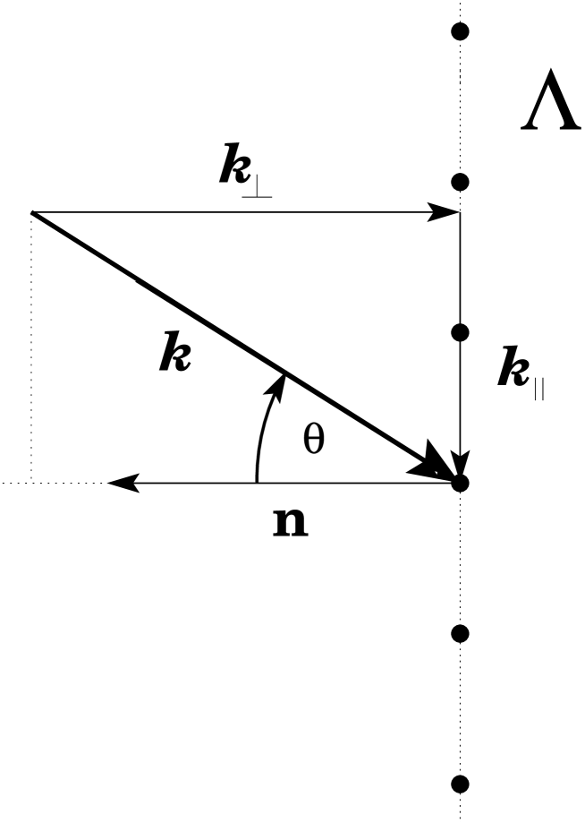
Figure 1:

Figure 2:

Figure 3:

Figure 4:

Figure 5:

References

- [1]
- [2] B. Segall, “Calculation of the band structure of “complex” crystals,” Phys. Rev. 105, 108-115 (1957).
- [3] F. S. Ham and B. Segall, “Energy bands in periodic lattices - Green’s function method,” Phys. Rev. 124, 1786-1796 (1961).
- [4] J. L. Beeby, “The diffraction of low-energy electrons by crystals,” J. Phys. C 1, 82-87 (1968).
- [5] K. Kambe, “Theory of Low-Energy Electron Diffraction. II. Cellular method for complex monolayers and multilayers,” Z. Naturforschg. 23a, 1280-1294 (1968).
- [6] K. Amemiya and K. Ohtaka, “Calculation of transmittance of light for an array of dielectric rods using vector cylindrical waves: Complex unit cells,” J. Phys. Soc. Jp. 72(5), 1244-1253 (2003).
- [7] O. X. Schlömilch, “Über die Bessel’schen Function,” Z. Math. Phys. 2, 137-165 (1857).
- [8] G. N. Watson, A Treatise on Theory of Bessel Functions, 2nd ed. (Cambrigde University Press, Cambrigde, 1966).
- [9] V. Twersky, “Elementary function representations of Schlömilch series,” Arch. Ration. Mech. Anal. 8, 323-332 (1961).
- [10] O. Emersleben, “Electrostatisches Gitter Potential,” Phys. Z. 24, 73-80 (1923).
- [11] P. Epstein, “Zur Theorie allgemeiner Zetafunktionen I,” Math. Ann. 56, 615-644 (1903).
- [12] M. L. Glasser and I. J. Zucker, “Lattice sums,” Theor. Chem. Adv. Perspectives 5, 67-139 (1980).
- [13] J. P. Buhler and R. E. Crandall, “On the convergence problem for lattice sums,” J. Phys. A: Math. Gen. 23, 2523-2528 (1990).
- [14] Yu. E. Karpeshina, “A decomposition theorem for the eigenfunctions of the problem of scattering by homogeneous periodic objects of chain type in three-dimensional space,” Sel. Math. Sov. 4(3), 259-276 (1985). Originally published in: Problems of Mathematical Physics, No. 10 [in Russian], State University Leningrad, 1982, pp. 137-163.
- [15] M. L. Glasser, “The evaluation of lattice sums. III. Phase modulated sums”, J. Math. Phys. 15, 188-189 (1974).
- [16] A. Grossmann, R. Høegh-Krohn, and M. Mebkhout, “The one particle theory of periodic point interactions. Polymers, monomolecular layers, and crystals,” Comm. Math. Phys. 77, 87-110 (1980).
- [17] M. Abramowitz and I. A. Stegun, Handbook of Mathematical Functions (Dover Publications, 1973).
- [18] W. von Ignatowsky, “Zur Theorie der Gitter,” Ann. Phys. (Leipzig) 44, 369-436 (1914).
- [19] P. P. Ewald, “Zur Begründung der Kristalloptik,” Ann. Phys. (Leipzig) 49, 1-38 (1916).
- [20] P. P. Ewald, “Die Berechnung optischer und elektrostatistischer Gitterpotentiale,” Ann. Phys. (Leipzig) 64, 253-287 (1921).
- [21] K. Kambe, “Theory of Low-Energy Electron Diffraction. I. Application of the Cellular method to monoatomic layers,” Z. Naturforschg. 22a, 322-330 (1967).
- [22] K. Kambe, “Theory of Electron Diffraction by Crystals. Green’s function and integral equation,” Z. Naturforschg. 22a, 422-431 (1967).
- [23] J. B. Pendry, Low Energy Electron Diffraction (Academic Press, London, 1974).
- [24] A. M. Ozorio de Almeida, “Real-space method for interpreting micrographs in cross-grating orientations. I. Exact wave-mechanical formulation,” Acta Cryst. A 31, 435-442 (1975). (In the expression (B.10) for , should be corrected to ).
- [25] M. V. Berry, “Quantizing a classically ergodic system: Sinai’s billiard and the KKR method,” Ann. Phys. (NY) 131, 163-216 (1981).
- [26] M. E. Veysoglu, H. A. Yueh, R. T. Shin, and J. A. Kong, “Polarimetric passive remote sensing of periodic surfaces,” J. Electromag. Waves Appl. 5(3), 267-280 (1991).
- [27] A. Moroz, “Exponentially convergent lattice sums,” Opt. Lett 26, 1119-1121 (2001). [See also Appendices A and B of the article by K. Ohtaka, T. Ueta, and K. Amemiya, “Calculation of photonic bands using vector cylindrical waves and reflectivity of light for an array of dielectric rods,” Phys. Rev. B 57, 2550-2568 (1998).]
- [28] A. Moroz, “On the computation of the free-space doubly-periodic Green’s function of the three-dimensional Helmholtz equation,” J. Electromagn. Waves Appl. 16, 457-465 (2002).
- [29] H. D. Maniar and J. N. Newman, “Wave diffraction by a long array of cylinders,” J. Fluid Mech. 339, 309-330 (1997).
- [30] C. M. Linton, “The Green’s function for the two-dimensional Helmholtz equation in periodic domains,” J. Eng. Math. 33, 377-402 (1998).
- [31] C. M. Linton, “Rapidly convergent representations for Green’s functions for Laplace’s equation,” Proc. R. Soc. London A 455, 1767-1797 (1999).
- [32] R. Porter and D. V. Evans, “Rayleigh-Bloch surface waves along periodic gratings and their connection with trapped modes in waveguides,” J. Fluid Mech. 386, 233-258 (1999).
- [33] N. Grønbech-Jensen, “Summation of logarithmic interactions in nonrectangular periodic media,” Comp. Phys. Commun. 119(2-3), 115-121 (1999).
- [34] N. A. Nicorovici and R. C. McPhedran, “Lattice sums for off-axis electromagnetic scattering by gratings,” Phys. Rev. E 50, 3143-3160 (1994).
- [35] J. P. Skinner and P. J. Collins, “A one-sided Poisson sum formula for semi-infinite array Green’s functions,” IEEE Trans. Antennas Propag. 45, 601-607 (1997).
- [36] K. Yasumoto and K. Yoshitomi, “Efficient calculation of lattice sums for free-space periodic Green s function,” IEEE Trans. Antennas Propag. 47, 1050-1055 (1999).
- [37] R. C. McPhedran, N. A. Nicorovici, L. C. Botten, and K. A. Grubits, “Lattice sums for gratings and arrays,” J. Math. Phys. 41, 7808-7816 (2000).
- [38] C. Craeye, A. B. Smolders, D. H. Schaubert, and A. G. Tijhuis, “An efficient computation scheme for the free space Green’s function of a two-dimensional semiinfinite phased array,” IEEE Trans. Antennas Propag. 51, 766-771 (2003).
- [39] I. D. Chremmos and N. Uzunoglu, “Integral equation analysis of propagation in a dielectric waveguide coupled to an infinite periodic sequence of ring resonators,” IEE Proc.-Sci. Meas. Technol. 151(6), 390-393 (2004).
- [40] M. L. Brongersma, J. W. Hartman, and H. A. Atwater, “Electromagnetic energy transfer and switching in nanoparticle chain arrays below the diffraction limit,” Phys. Rev. B 62, R16356-R16359 (2000).
- [41] S. A. Maier, P. G. Kik, and H. A. Atwater, “Optical pulse propagation in metal nanoparticle chain waveguides,” Phys. Rev. B 67, 205402 (2003).
- [42] V. N. Astratov, J. P. Franchak, and S. P. Ashili, “Optical coupling and transport phenomena in chains of spherical dielectric microresonators with size disorder,” Appl. Phys. Lett. 85, 5508-5510 (2004).
- [43] R. Shore and A. D. Yaghjian, “Traveling electromagnetic waves on linear periodic arrays of lossless penetrable spheres,” IEICE Trans. Commun. E88-B(6), 2346-2352 (2005).
- [44] M. Quinten, A. Leitner, J. R. Krenn, and F. R. Aussenegg, “Electromagnetic energy transport via linear chains of silver nanoparticles,” Opt. Lett. 23, 1331-1333 (1998).
- [45] S.-Y. Park and D. Stroud, “Surface-plasmon dispersion relations in chains of metallic nanoparticles: An exact quasistatic calculation,” Phys. Rev. B 69, 125418 (2004).
- [46] W. H. Weber and G. W. Ford, “Propagation of optical excitations by dipolar interactions in metal nanoparticle chains,” Phys. Rev. B 70, 125429 (2004).
- [47] J. M. Gérardy and M. Ausloos, “Absorption spectrum of clusters of spheres from the general solution of Maxwell’s equations. II. Optical properties of aggregated metal spheres,” Phys. Rev. B 25, 4204-4229 (1982).
- [48] Yu. E. Karpeshina, “The spectrum and eigenfunctions of the Schrödinger operator in three-dimensional space with point potential of the type of a homogeneous two-dimensional lattice,” Teor. Mat. Fyz. 57, 414-423 (1983).
- [49] E. T. Whittaker and G. N. Watson, A Course of Modern Analysis, (Cambrigde University Press, Cambrigde, 1965).
- [50] E. G. McRae, “Multiple-scattering treatment of low-energy electron-diffraction intensities,” J. Chem. Phys. 45, 3258-3276 (1966).
- [51] W. H. Butler, “One-dimensional model for transition metals and their alloys,” Phys. Rev. B 14, 468-477 (1976).
- [52] D. J. Griffihs and C. A. Steinke, “Waves in locally periodic media,” Am. J. Phys. 69, 137-154 (2001).
- [53] J. Lekner, “Summation of dipolar fields in simulated liquid-vapour interfaces,” Physica A 157(2), 826-838 (1989).
- [54] A. Y. Toukmaji and J.A. Board Jr., “Ewald summation techniques in perspective: a survey,” Comp. Phys. Commun. 95, 73-92 (1996).
- [55] W. Kohn and N. Rostoker, “Solution of the Schrödinger equation in periodic lattices with an application to metallic lithium,” Phys. Rev. 94, 1111-1120 (1954).
- [56] J. Korringa, “On the calculation of the energy of a Bloch wave in a metal,” Physica 13, 392-400 (1947).
- [57] J. S. Faulkner, “Multiple scattering calculation in two dimensions,” Phys. Rev. B 38, 1686-1694 (1988).
- [58] R. G. Newton, “Bloch-wave scattering by crystal defects,” J. Math. Phys. 32, 551-560 (1991).
- [59] A. Gonis, Green functions for ordered and disordered systems, Studies in mathematical physics (North-Holland, Amsterdam, 1992).
- [60] X. Wang, X.-G. Zhang, Q. Yu, and B. N. Harmon, “Multiple-scattering theory for electromagnetic waves,” Phys. Rev. B 47, 4161-4167 (1993).
- [61] A. Moroz, “Density-of-states calculation and multiple scattering theory for photons,” Phys. Rev. B 51, 2068-2081 (1995).
- [62] A. Moroz and C. Sommers, “Photonic band gaps of three-dimensional face-centered cubic lattices,” J. Phys.: Condens. Matter 11, 997-1008 (1999).
- [63] H. van der Lem and A. Moroz, “Towards two-dimensional complete photonic band gap structures below infrared wavelengths,” J. Opt. A: Pure Appl. Opt. 2, 395-399 (2000).
- [64] A. Moroz, “Three-dimensional complete photonic-bandgap structures in the visible,” Phys. Rev. Lett. 83, 5274-5279 (1999).
- [65] M. Kafesaki and E. N. Economou, “Multiple-scattering theory for three-dimensional periodic acoustic composites,” Phys. Rev. B 60, 11993-12001 (1999).
- [66] A. Moroz, “Metallo-dielectric diamond and zinc-blende photonic crystals,” Phys. Rev. B 66, 115109 (2002).
- [67] S. Y. Tong, “Theory of low-energy electron diffraction,” Prog. Surf. Sci. 7, 1-48 (1975).
- [68] J. M. McLaren, S. Crampin, D. D. Vvedensky, R. C. Albers, and J. B. Pendry, “Layer KKR electronic structure code for bulk and interface geometries,” Comp. Phys. Commun. 60, 365-389 (1990).
- [69] K. Ohtaka, “Scattering theory of low-energy photon diffraction,” J. Phys. C 13, 667-680 (1980).
- [70] A. Modinos, “Scattering of electromagnetic waves by a plane of spheres-formalism,” Physica 141, 575-588 (1987).
- [71] N. Stefanou, V. Karathanos, and A. Modinos, ““Scattering of electromagnetic waves by periodic structures,” J. Phys.: Condens. Matter 4, 7389-7400 (1992).
- [72] D. Maystre, Electromagnetic study of photonic band gaps,” Pure Appl. Opt. 3, 975-993 (1994).
- [73] V. Yannopapas, N. Stefanou, and A. Modinos, “Heterostructures of photonic crystals: frequency bands and transmission coefficients,” Comp. Phys. Commun. 113, 49-77 (1998).
- [74] I. E. Psarobas, N. Stefanou, and A. Modinos, “Scattering of elastic waves by periodic arrays of spherical bodies,” Phys. Rev. B 62, 278-291 (2000).
- [75] V. Poborchii, T. Tada, T. Kanayama, and A. Moroz, “Silver-coated silicon-pillar photonic crystals: enhancement of a photonic band gap,” Appl. Phys. Lett. 82, 508-510 (2003).
- [76] H.-J. Stöckmann, Quantum Chaos - An Introduction (Cambridge University Press, Cambridge, 1999).
- [77] S. Albeverio, F. Gesztesy, R. Høegh-Krohn, and H. Holden, Solvable Models in Quantum Mechanics (Heidelberg, Springer, 1988).
- [78] A. P. Prudnikov, Yu. A. Brychkov, and O. I. Marichev, Integrals and Series, 2nd ed. (Gordon and Breach, London, 1988).
- [79] I. S. Gradshteyn and I. M. Ryzhik, Table of Integrals, Series and Products, 4th ed. (Academic, New York, 1980).
- [80] M. Reed and B. Simon, Scattering Theory (Academic Press, New York, 1979).
- [81] S. Stein, “Addition theorems for spherical wave functions,” Quart. Appl. Math. 19, 15-24 (1961).
- [82] C. M. Linton, “Schlömilch series that arise in diffraction theory and their efficient computation,” J. Phys. A 39, 3325-3340 (2006).