Algebraic and geometric structures of
Special Relativity

Abstract

I review, on an advanced level, some of the algebraic and geometric structures that underlie the theory of Special Relativity. This includes a discussion of relativity as a symmetry principle, derivations of the Lorentz group, its composition law, its Lie algebra, comparison with the Galilei group, Einstein synchronization, the lattice of causally and chronologically complete regions in Minkowski space, rigid motion (the Noether-Herglotz theorem), and the geometry of rotating reference frames. Representation-theoretic aspects of the Lorentz group are not included. A series of appendices present some related mathematical material.

This paper is a contribution to the proceedings of the 339th WE-Heraeus-Seminar Special Relativity: Will it Survive the Next 100 Years?, edited by J. Ehlers and C. Lämmerzahl, which will be published by Springer Verlag in 2006.

1 Introduction

In this contribution I wish to discuss some structural aspects of Special Relativity (henceforth abbreviated SR) which are, technically speaking, of a more advanced nature. Most of what follows is well known, though generally not included in standard text-book presentations. Against my original intention, I decided to not include those parts that relate to the representation- and field-theoretic aspects of the homogeneous and inhomogeneous Lorentz group, but rather to be more explicit on those topics now covered. Some of the abandoned material is (rather informally) discussed in [27]. All of it will appear in [22]. For a comprehensive discussion of many field-theoretic aspects, see e.g. [42].

I always felt that Special Relativity deserves more attention than what is usually granted to it in courses on mechanics or electrodynamics. There is a fair amount of interesting algebraic structure that characterizes the transition between the Galilei and Lorentz group, and likewise there is some interesting geometry involved in the transition between Newtonian (or Galilean) spacetime and Minkowski space. The latter has a rich geometric structure, notwithstanding the fact that, from a general relativistic viewpoint, it is ‘just’ flat spacetime. I hope that my contribution will substantiate these claims. For the convenience of some interested readers I have included several mathematical appendices with background material that, according to my experience, is considered helpful being spelled out in some detail.

2 Some remarks on ‘symmetry’ and ‘covariance’

For the purpose of this presentation I regard SR as the (mathematical) theory of how to correctly implement the Galilean Relativity Principle—henceforth simply abbreviated by RP. The RP is a physical statement concerning a subclass of phenomena—those not involving gravity—which translates into a mathematical symmetry requirement for the laws describing them. But there is no unique way to proceed; several choices need to be made whose correctness cannot be decided by mere logic.

Given that the symmetry requirement is implemented by a group action (which may be relaxed; compare e.g. supersymmetry, which is not based on a group), the most fundamental question is: what group? In this regard there is quite a convincing string of arguments that, given certain mild technical assumptions, the RP selects either the Galilei or the Lorentz group (the latter for some yet undetermined velocity parameter $c$). This will be discussed in detail in Section 3.

Almost as important as the selection of a group is the question of how it should act on physical entities in question, like particles and fields. The importance and subtlety of this question is usually underestimated. Let us therefore dwell a little on it.

As an example we consider vacuum electrodynamics. Here the mathematical objects that represent physical reality are two spacetime dependent fields, $\vec{E}(\vec{x},t)$ and $\vec{B}(\vec{x},t)$, which take values in a vector space isomorphic to $\mathbb{R}^{3}$. There will be certain technical requirements on these fields, e.g. concerning differentiability and fall-off at spatial infinity, which we do not need to spell out here. For simplicity we shall assume that the set of all fields obeying these conditions forms an infinite-dimensional linear space $\mathcal{K}$, which is sometimes called the space of ‘kinematical’ (or ‘kinematically possible’) fields. Those fields in $\mathcal{K}$ which satisfy Maxwell’s (vacuum) equations form a proper subset, $\mathcal{S}\subset\mathcal{K}$, which, due to the linearity of the equations and the boundary conditions (fall-off to zero value, say), is a linear subspace. It is called the space of ‘physical’ (or ‘dynamically possible’) fields. Clearly these notions of the spaces of kinematically and dynamically possible fields apply to all sorts of situations in physics where one considers ‘equations of motion’, though in general neither of these sets will be a vector space. This terminology was introduced in [2].

In general, we say that a group $G$ is a symmetry group of a given dynamical theory if the following two conditions are satisfied:

• There exists an (say left-) effective action $G\times\mathcal{K}\rightarrow\mathcal{K}$, $(g,k)\mapsto g\cdot k$, of $G$ on $\mathcal{K}$ (cf. Sect. A.1). Posing effectiveness just means that we do not wish to allow trivial enlargements of the group by elements that do not move anything. It also means no loss of generality, since any action of a group $G$ on a set $\mathcal{K}$ factors through an effective action of $G/G^{\prime}$ on $\mathcal{K}$, where $G^{\prime}$ is the normal subgroup of trivially acting elements (cf. Sect. A.1). Such an action of the group on the kinematical space of physical fields is also called an implementation of the group into the physical theory.

• The action of $G$ on $\mathcal{K}$ leaves $\mathcal{S}$ invariant (as a set, not necessarily pointwise), i.e. if $s\in\mathcal{S}$ then $g\cdot s\in\mathcal{S}$ for all $g$. This merely says that the group action restricts from $\mathcal{K}$ to $\mathcal{S}$. Note that, from an abstract point of view, this is the precise statement of the phrase ‘leaving the field equations invariant’, since the field equations are nothing but a characterization of the subset $\mathcal{S}\subset\mathcal{K}$.

If this were all there is to require for a group to count as a symmetry group, then we would probably be surprised by the wealth of symmetries in Nature. For example, in the specific case at hand, vacuum electrodynamics, we often hear or read the statement that the Lorentz group leaves Maxwell’s equations invariant, whereas the Galilei group does not. Is this really true? Has anyone really shown in this context that the Galilei group cannot effectively act on $\mathcal{K}$ so as to leave $\mathcal{S}$ invariant? Certainly not, because such an action is actually known to exist; see e.g. Chap. 5.9 in [21]. Hence, in the general sense above, the Galilei group is a symmetry group of Maxwell’s equations!

The folklore statement just alluded to can, however, be turned into a true statement if a decisive restriction for the action is added, namely that it be local. This means that the action on the space of fields is such that the value of the transformed field at the transformed spacetime point depends only on the value of the untransformed field at the untransformed point and not, in addition, on its derivatives. This is the crucial assumption that is implicit in all proofs of Galilean-non-invariance of Maxwell’s equations and that is also made regarding the Lorentz group in classical and quantum field theories. The action of the Galilei group that makes it a symmetry group for Maxwell’s equations is, in fact, such that the transformed field depends linearly on the original field and its derivatives to all orders. That is, it is highly non local.

Returning to the general discussion, we now consider a classical field, that is, a map $\Psi:M\rightarrow V$ from spacetime $M$ into a vector space $V$. A spacetime symmetry-group has an action on $M$, denoted by $T:(g,x)\mapsto T_{g}(x)$, as well as an action on $V$, which in most cases of interest is a linear representation $g\mapsto D(g)$ of $G$. A local action of $G$ on field space is then given by

$$(g,\Psi)\mapsto g\cdot\Psi:=D(g)\circ\Psi\circ T_{g}^{-1}\,,$$ (1)

where here and below the symbol $\circ$ denotes composition of maps. This is the form of the action one usually assumes. Existing generalizations concerning possible non-linear target spaces for $\Psi$ and/or making $\Psi$ a section in a bundle, rather than just a global function, do not influence the locality aspect emphasized here and will be ignored.

Next to fields one also considers particles, at least in the classical theory. Structureless (e.g. no spin) particles in spacetime are mathematically idealized by maps $\gamma:\mathbb{R}\rightarrow M$, where $\mathbb{R}$ (or a subinterval thereof) represents parameter space. The parameterization usually does not matter, except for time orientation, so any reparameterization $f:\mathbb{R}\rightarrow\mathbb{R}$ with $f^{\prime}>0$ gives a reparameterized curve $\gamma^{\prime}:=\gamma\circ f$ which is just as good. On the space of particles, the group $G$ acts as follows:

$$(g,\gamma)\mapsto g\cdot\gamma:=T_{g}\circ\gamma\,.$$ (2)

Together (1) and (2) define an action on all the dynamical entities, that is particles and fields, which we collectively denote by the symbol $\Phi$. The given action of $G$ on that space is simply denoted by $(g,\Phi)\mapsto g\cdot\Phi$.

Now, the set of equations of motion for the whole system can be written in the general form

$$\mathcal{E}[\Sigma,\Phi]=0\,,$$ (3)

where this should be read as a multi-component equation (with $0$ being the zero ‘vector’ in target space). $\Sigma$ stands collectively for non-dynamical entities (background structures) whose values are fixed by means independent of equation (3). It could, for example, be the Minkowski metric in Maxwell’s equations and also external currents. The meaning of (3) is to determine $\Phi$, given $\Sigma$ (and the boundary conditions for $\Phi$). We stress that $\Sigma$ is a constitutive part of the equations of motion. We now make the following

Definition 1.

An action of the group $G$ on the space of dynamical entities $\Phi$ is said to correspond to a symmetry of the equations of motion iff for all $g\in G$ we have

$$\mathcal{E}[\Sigma,\Phi]=0\ \Longleftrightarrow\ \mathcal{E}[\Sigma,g\cdot\Phi]=0\,.$$ (4)

Different form that is mere ‘covariance’, which is a far more trivial requirement. It arises if the space of background structures, $\Sigma$, also carries an action of $G$ (as it naturally does if the $\Sigma$ are tensor fields). Then we have

Definition 2.

An action of the group $G$ on the space of dynamical and non-dynamical entities $\Phi$ and $\Sigma$ is said to correspond to a covariance of the equations of motion iff for all $g\in G$ we have

$$\mathcal{E}[\Sigma,\Phi]=0\ \Longleftrightarrow\ \mathcal{E}[g\cdot\Sigma,g\cdot\Phi]=0\,.$$ (5)

The difference to symmetries is that the background structures—and in that sense the equations of motion themselves—are changed too. Equation (4) says that if $\Phi$ solves the equations of motion then $g\cdot\Phi$ solves the very same equations. In contrast, (5) merely tells us that if $\Phi$ solves the equations of motion then $g\cdot\Phi$ solves the appropriately transformed equations. Trivially, a symmetry is also a covariance but the converse it not true. Rather, a covariance is a symmetry iff it stabilizes the background structures, i.e. if for all $g\in G$ we have $g\cdot\Sigma=\Sigma$.

Usually one has a good idea of what the dynamical entities $\Phi$ in ones theory should be, whereas the choice of $\Sigma$ is more a matter of presentation and therefore conventional. After all, the only task of equations of motion is to characterize the set $\mathcal{S}$ of dynamically possible fields (and particles) amongst the set $\mathcal{K}$ of all kinematically possible ones. Whether this is done by using auxiliary structures $\Sigma_{1}$ or $\Sigma_{2}$ should not affect the physics. It is for this reason that one has to regard the requirement of mere covariance as, physically speaking, rather empty. This is because one can always achieve covariance by suitably adding non-dynamical structures $\Sigma$. Let us give an example for this [2].

Consider the familiar heat equation,

$$\partial_{t}T-\kappa\Delta T=0\,.$$ (6)

Here the dynamical field $\Phi=T$ is the temperature function. The background structure is the 3-dimensional Euclidean metric, $\delta$, of space which enters the Laplacian, $\Delta:=\delta^{ab}\partial_{a}\partial_{b}$; hence $\Sigma=\delta$. This equation possesses time translations and Euclidean motions in space (we neglect space reflections for simplicity) as symmetries. These form the group $E_{3}\cong\mathbb{R}^{3}\rtimes SO(3)$, the semi-direct product of spatial translations and rotations. Clearly $E_{3}$ stabilizes $\delta$.

But without changing the physics we can rewrite (6) in the following spacetime form: Let $(x^{0},x^{1},x^{2},x^{3})=(ct,x,y,z)$ be inertial coordinates in Minkowski space and $n=\partial_{t}=n^{\mu}\partial_{\mu}$ (i.e. $n^{\mu}=(c,0,0,0)$) the (covariant) constant vector field describing the motion of the inertial observer. The components of the Minkowski metric in these coordinates are denoted by $g_{\mu\nu}$. In our conventions (‘mostly minus’) $\{g_{\mu\nu}\}=\text{diag(1,-1,-1,-1)}$. Then (6) is clearly just the same as

$$n^{\mu}\partial_{\mu}T-\kappa\left(c^{-2}\,n^{\mu}n^{\nu}-g^{\mu\nu}\right)\,\partial_{\mu}\partial_{\nu}\,T=0\,.$$ (7)

Here the dynamical variable is still $\Phi=T$ but the background variables are now given by $\Sigma=(n,g)$. This equations is now manifestly covariant under the Lorentz group if $n^{\mu}$ and $g^{\mu\nu}$ are acted upon as indicated by their indices. Hence we were able to enlarge the covariance group by enlarging the space of $\Sigma$s. In fact, we could even make the equation covariant under general diffeomorphisms by replacing partial with covariant derivatives. But note that the symmetry group would still be that subgroup that stabilizes (leaves invariant) the (flat) metric $g$ and the (covariant constant) vector field $n$, which again results in the same symmetry group as for the original equation (6). For more discussion concerning also the problematic aspects of of the notion of ‘general covariance’, see e.g. [23].

3 The impact of the relativity principle on the
automorphism group of spacetime

In the history of SR it has often been asked what the most general transformations of spacetime were that implemented the relativity principle (RP), without making use of the requirement of the constancy of the speed of light. This question was first addressed by Ignatowsky [31], who showed that under a certain set of technical assumptions (not consistently spelled out by him) the RP alone suffices to arrive at a spacetime symmetry group which is either the Galilei or the Lorentz group, the latter for some yet undetermined limiting velocity $c$. More precisely, what is actually shown in this fashion is, as we will see, that the spacetime symmetry group must contain either the proper orthochronous Galilei or Lorentz group, if the group is required to comprise at least spacetime translations, spatial rotations, and boosts (velocity transformations). What we hence gain is the group-theoretic insight of how these transformations must combine into a common group, given that they form a group at all. We do not learn anything about other transformations, like spacetime reflections or dilations, whose existence we neither required nor ruled out on this theoretical level.

The work of Ignatowsky was put into a logically more coherent form by Franck & Rothe [19][20], who showed that some of the technical assumptions could be dropped. Further formal simplifications were achieved by Berzi & Gorini [8]. Below we shall basically follow their line of reasoning, except that we do not impose the continuity of the transformations as a requirement, but conclude it from their preservation of the inertial structure plus bijectivity. See also [3] for an alternative discussion on the level of Lie algebras.

The principles of SR are mathematically most concisely expressed in terms of few simple structures put onto spacetime. In SR these structures are absolute in the sense of not being subject to any dynamical change. From a fundamental point of view, it seems rather a matter of convention whether one thinks of these structures as primarily algebraic or geometric. According to the idea advocated by Felix Klein in his ‘Erlanger Programm’ [36], a geometric structure can be characterized by its automorphism group. The latter is generally defined by the subgroup of bijections of the set in question which leaves the geometric structure—e.g. thought of as being given in terms of relations—invariant. Conversely, any transformation group (i.e. subgroup of group of bijections) can be considered as the automorphism group of some ‘geometry’ which is defined via the invariant relations.

The geometric structure of spacetime is not a priori given to us. It depends on the physical means on which we agree to measure spatial distances and time durations. These means refer to physical systems, like ‘rods’ and ‘clocks’, which are themselves subject to dynamical laws in spacetime. For example, at a fundamental physical level, the spatial transportation of a rod or a clock from one place to another is certainly a complicated dynamical process. It is only due to the special definition of ‘rod’ and ‘clock’ that the result of such a process can be summarized by simple kinematical rules. Most importantly, their dynamical behavior must be ‘stable’ in the sense of being essentially independent of their dynamical environment. Hence there is always an implicit consistency hypothesis underlying operational definitions of spatio-temporal measurements, which in case of SR amount to the assumption that rods and clocks are themselves governed by Lorentz invariant dynamical laws.

A basic physical law is the law of inertia. It states the preference of certain types of motions for force-free, uncharged, zero-spin test-particles: the ‘uniform’ and ‘rectilinear’ ones. In the spacetime picture this corresponds to the preference of certain curves corresponding to the inertial worldlines of the force-free test particles. In the gravity-free case, we model these world lines by straight lines of the affine space $\mathrm{Aff}(\mathbb{R}^{4})$ over the vector space $\mathbb{R}^{4}$. This closely corresponds to our intuitive notion of homogeneity of space and time, that is, that there exists an effective and transitive (and hence simply transitive) action of the Abelian group $\mathbb{R}^{4}$ of translations (cf. Sects. A.1 and A.7). A lot could (and perhaps should) be said at this point about the proper statement of the law of inertia and precisely how it endows spacetimes with certain geometric structures. Instead we will simply refer the interested reader to the literature; see e.g. [26] and references therein.

Note that we do not conversely assume any straight line to correspond to some inertial world-line. Hence the first geometric structure on spacetime, which can be thought of as imposed by the law of inertia, is that of a subset of straight lines. If all straight lines were involved, the automorphism group of spacetime would necessarily have to map any straight line to a straight line and therefore be a subgroup of the affine group $\mathbb{R}^{4}\rtimes\mathsf{GL}(4,\mathbb{R})$. This is just the content of the main theorem in affine geometry; see e.g. [6]. However, we can only argue that it must map the subset of inertial world-lines onto itself. We take this subset to consist of all straight lines in $\mathrm{Aff}(\mathbb{R}^{4})$ whose slope with respect to some reference direction is smaller than a certain finite value $\beta$. This corresponds to all worldlines not exceeding a certain limiting speed with reference to some inertial frame. It is then still true that any bijection of $\mathrm{Aff}(\mathbb{R}^{4})$ preserving that subset must be a subgroup of the affine group [29]. Also, it is not necessary to assume that lines map surjectively onto lines [16].

For further determination of the automorphism group of spacetime we invoke the following principles:

• Homogeneity of spacetime.

• Isotropy of space.

• Galilean principle of relativity.

We take ST1 to mean that the sought-for group should include all translations and hence be of the form $\mathbb{R}^{4}\rtimes\mathsf{G}$, where $\mathsf{G}$ is a subgroup of $\mathsf{GL}(4,\mathbb{R})$. ST2 is interpreted as saying that $G$ should include the set of all spatial rotations. If, with respect to some frame, we write the general element $A\in\mathsf{GL}(4,\mathbb{R})$ in a $1+3$ split form (thinking of the first coordinate as time, the other three as space), we want $\mathsf{G}$ to include all

$$R(\mathbf{D})=\begin{pmatrix}1&\vec{0}^{\top}\\ \vec{0}&\mathbf{D}\end{pmatrix}\,,\qquad\text{where}\quad\mathbf{D}\in\mathsf{SO}(3)\,.$$ (8)

Finally, ST3 says that velocity transformations, henceforth called ‘boosts’, are also contained in $\mathsf{G}$. However, at this stage we do not know how boosts are to be represented mathematically. Let us make the following assumptions:

• Boosts $B(\vec{v})$ are labeled by a vector $\vec{v}\in B_{c}(\mathbb{R}^{3})$, where $B_{c}(\mathbb{R}^{3})$ is the open ball in $\mathbb{R}^{3}$ of radius $c$. The physical interpretation of $\vec{v}$ shall be that of the boost velocity, as measured in the system from which the transformation is carried out. We allow $c$ to be finite or infinite ($B_{\infty}(\mathbb{R}^{3})=\mathbb{R}^{3}$). $\vec{v}=\vec{0}$ corresponds to the identity transformation, i.e. $B(\vec{0})=\text{id}_{\mathbb{R}^{4}}$. We also assume that $\vec{v}$, considered as coordinate function on the group, is continuous.

• As part of ST2 we require equivariance of boosts under rotations:

  $$R(\mathbf{D})\cdot B(\vec{v})\cdot R(\mathbf{D}^{-1})=B(\mathbf{D}\cdot\vec{v})\,.$$ (9)

The latter assumption allows us to restrict attention to boost in a fixed direction, say that of the positive $x$-axis. Once their analytical form is determined as function of $v$, where $\vec{v}=v\vec{e}_{x}$, we deduce the general expression for boosts using (9) and (8). We make no assumptions involving space reflections. We now restrict attention to $\vec{v}=v\vec{e}_{x}$. We wish to determine the most general form of $B(\vec{v})$ compatible with all requirements put so far. We proceed in several steps:

1. Using an arbitrary rotation $\mathbf{D}$ around the $x$-axis, so that $\mathbf{D}\cdot\vec{v}=\vec{v}$, equation (9) allows to prove that

   $$B(v\vec{e}_{x})=\begin{pmatrix}\mathbf{A}(v)&0\\ 0&\alpha(v)\mathbf{1}_{2}\end{pmatrix}\,,$$ (10)

   where here we wrote the $4\times 4$ matrix in a $2+2$ decomposed form. (i.e. $\mathbf{A}(v)$ is a $2\times 2$ matrix and $\mathbf{1}_{2}$ is the $2\times 2$ unit-matrix). Applying (9) once more, this time using a $\pi$-rotation about the $y$-axis, we learn that $\alpha$ is an even function, i.e.

   $$\alpha(v)=\alpha(-v)\,.$$ (11)

   Below we will see that $\alpha(v)\equiv 1$.

2. Let us now focus on $\mathbf{A}(v)$, which defines the action of the boost in the $t-x$ plane. We write

   $$\begin{pmatrix}t\\ x\end{pmatrix}\mapsto\begin{pmatrix}t^{\prime}\\ x^{\prime}\end{pmatrix}=\mathbf{A}(v)\cdot\begin{pmatrix}t\\ x\end{pmatrix}=\begin{pmatrix}a(v)&b(v)\\ c(v)&d(v)\end{pmatrix}\cdot\begin{pmatrix}t\\ x\end{pmatrix}\,.$$ (12)

   We refer to the system with coordinates $(t,x)$ as $K$ and that with coordinates $(t^{\prime},x^{\prime})$ as $K^{\prime}$. From (12) and the inverse (which is elementary to compute) one infers that the velocity $v$ of $K^{\prime}$ with respect to $K$ and the velocity $v^{\prime}$ of $K$ with respect to $K^{\prime}$ are given by

   $$v\, =\, -\,c(v)/d(v)\,,$$ (13a)

   $$v^{\prime}\, =\, -\,v\,d(v)/a(v)\,=:\,\varphi(v)\,.$$ (13b)

   Since the transformation $K^{\prime}\rightarrow K$ is the inverse of $K\rightarrow K^{\prime}$, the function $\varphi:(-c,c)\rightarrow(-c,c)$ obeys

   $$\mathbf{A}(\varphi(v))=(\mathbf{A}(v))^{-1}\,.$$ (14)

   Hence $\varphi$ is a bijection of the open interval $(-c,c)$ onto itself and obeys

   $$\varphi\circ\varphi=\text{id}_{(-c,c)}\,.$$ (15)

3. Next we determine $\varphi$. Once more using (9), where $\mathbf{D}$ is a $\pi$-rotation about the $y$-axis, shows that the functions $a$ and $d$ in (10) are even and the functions $b$ and $c$ are odd. The definition (13b) of $\varphi$ then implies that $\varphi$ is odd. Since we assumed $\vec{v}$ to be a continuous coordinatization of a topological group, the map $\varphi$ must also be continuous (since the inversion map, $g\mapsto g^{-1}$, is continuous in a topological group). A standard theorem now states that a continuous bijection of an interval of $\mathbb{R}$ onto itself must be strictly monotonic. Together with (15) this implies that $\varphi$ is either the identity or minus the identity map. If it is the identity map, evaluation of (14) shows that either the determinant of $\mathbf{A}(v)$ must equals $-1$, or that $\mathbf{A}(v)$ is the identity for all $\vec{v}$. We exclude the second possibility straightaway and the first one on the grounds that we required $\mathbf{A}(v)$ be the identity for $v=0$. Also, in that case, (14) implies $A^{2}(v)=\text{id}$ for all $v\in(-c,c)$. We conclude that $\varphi=-\text{id}$, which implies that the relative velocity of $K$ with respect to $K^{\prime}$ is minus the relative velocity of $K^{\prime}$ with respect to $K$. Plausible as it might seem, there is no a priori reason why this should be so.. On the face of it, the RP only implies (15), not the stronger relation $\varphi(v)=-v$. This was first pointed out in [8].

4. We briefly revisit (11). Since we have seen that $B(-v\vec{e}_{x})$ is the inverse of $B(v\vec{e}_{x})$, we must have $\alpha(-v)=1/\alpha(v)$, so that (11) implies $\alpha(v)\equiv\pm 1$. But only $\alpha(v)\equiv+1$ is compatible with our requirement that $B(\vec{0})$ be the identity.

5. Now we return to the determination of $\mathbf{A}(v)$. Using (13) and $\varphi=-\text{id}$, we write

   $$\mathbf{A}(v)=\begin{pmatrix}a(v)&b(v)\\ -va(v)&a(v)\end{pmatrix}$$ (16)

   and

   $$\Delta(v):=\det\bigl{(}\mathbf{A}(v)\bigr{)}=a(v)\bigl{[}a(v)+vb(v)\bigr{]}\,.$$ (17)

   Equation $\mathbf{A}(-v)=(\mathbf{A}(v))^{-1}$ is now equivalent to

   $$a(-v) \,=\,a(v)/\Delta(v)\,,$$ (18a)

   $$b(-v) \,=\,-\,b(v)/\Delta(v)\,.$$ (18b)

   Since, as already seen, $a$ is an even and $b$ is an odd function, (18) is equivalent to $\Delta(v)\equiv 1$, i.e. the unimodularity of $B(\vec{v})$. Equation (17) then allows to express $b$ in terms of $a$:

   $$b(v)=\frac{a(v)}{v}\left[\frac{1}{a^{2}(v)}-1\right]\,.$$ (19)

6. Our problem is now reduced to the determination of the single function $a$. This we achieve by employing the requirement that the composition of two boosts in the same direction results again in a boost in that direction, i.e.

   $$\mathbf{A}(v)\cdot\mathbf{A}(v^{\prime})=\mathbf{A}(v^{\prime\prime})\,.$$ (20)

   According to (16) each matrix $\mathbf{A}(v)$ has equal diagonal entries. Applied to the product matrix on the left hand side of (20) this implies that $v^{-2}(a^{-2}(v)-1)$ is independent of $v$, i.e. equal to some constant $k$ whose physical dimension is that of an inverse velocity squared. Hence we have

   $$a(v)=\frac{1}{\sqrt{1+kv^{2}}}\,,$$ (21)

   where we have chosen the positive square root since we require $a(0)=1$. The other implications of (20) are

   $$a(v)a(v^{\prime})(1-kvv^{\prime}) \,=\,a(v^{\prime\prime})\,,$$ (22a)

   $$a(v)a(v^{\prime})(1+vv^{\prime}) \,=\,v^{\prime\prime}a(v^{\prime\prime})\,,$$ (22b)

   from which we deduce

   $$v^{\prime\prime}=\frac{v+v^{\prime}}{1-kvv^{\prime}}\,.$$ (23)

   Conversely, (21) and (23) imply (22). We conclude that (20) is equivalent to (21) and (23).

7. So far a boost in $x$ direction has been shown to act non-trivially only in the $t-x$ plane, where its action is given by the matrix that results from inserting (19) and (21) into (16):

   $$\mathbf{A}(v)=\begin{pmatrix}a(v)&kv\,a(v)\\ -v\,a(v)&a(v)\,,\end{pmatrix}\qquad\text{where}\quad a(v)=1/\sqrt{1+kv^{2}}\,.$$ (24)

   • If $k>0$ we rescale $t\mapsto\tau:=t/\sqrt{k}$ and set $\sqrt{k}\,v:=\tan\alpha$. Then (24) is seen to be a Euclidean rotation with angle $\alpha$ in the $\tau-x$ plane. The velocity spectrum is the whole real line plus infinity, i.e. a circle, corresponding to $\alpha\in[0,2\pi]$, where $0$ and $2\pi$ are identified. Accordingly, the composition law (23) is just ordinary addition for the angle $\alpha$. This causes several paradoxa when $v$ is interpreted as velocity. For example, composing two finite velocities $v,v^{\prime}$ which satisfy $vv^{\prime}=1/k$ results in $v^{\prime\prime}=\infty$, and composing two finite and positive velocities, each of which is greater than $1/\sqrt{k}$, results in a finite but negative velocity. In this way the successive composition of finite positive velocities could also result in zero velocity. The group $\mathsf{G}\subset\mathsf{GL}(n,\mathbb{R})$ obtained in this fashion is, in fact, $\mathsf{SO}(4)$. This group may be uniquely characterized as the largest connected group of bijections of $\mathbb{R}^{4}$ that preserves the Euclidean distance measure. In particular, it treats time symmetrically with all space directions, so that no invariant notion of time-orientability can be given in this case.

   • For $k=0$ the transformations are just the ordinary boosts of the Galilei group. The velocity spectrum is the whole real line (i.e. $v$ is unbounded but finite) and $\mathsf{G}$ is the Galilei group. The law for composing velocities is just ordinary vector addition.

   • Finally, for $k<0$, one infers from (23) that $c:=1/\sqrt{-k}$ is an upper bound for all velocities, in the sense that composing two velocities taken from the interval $(-c,c)$ always results in a velocity from within that interval. Writing $\tau:=ct$, $v/c=:\beta=:\tanh\rho$, and $\gamma=1/\sqrt{1-\beta^{2}}$, the matrix (24) is seen to be a Lorentz boost or hyperbolic motion in the $\tau-x$ plane:

     $$\begin{pmatrix}\tau\\ x\end{pmatrix}\mapsto\begin{pmatrix}\gamma&-\beta\gamma\\ -\beta\gamma&\gamma\end{pmatrix}\cdot\begin{pmatrix}\tau\\ x\end{pmatrix}=\begin{pmatrix}\cosh\rho&-\sinh\rho\\ -\sinh\rho&\cosh\rho\end{pmatrix}\cdot\begin{pmatrix}\tau\\ x\end{pmatrix}\,.$$ (25)

     The quantity

     $$\rho:=\tanh^{-1}(v/c)=\tanh^{-1}(\beta)$$ (26)

     is called rapidity. If rewritten in terms of the corresponding rapidities the composition law (23) reduces to ordinary addition: $\rho^{\prime\prime}=\rho+\rho^{\prime}$.

This shows that only the Galilei and the Lorentz group survive as candidates for any symmetry group implementing the RP. Once the Lorentz group for velocity parameter $c$ is chosen, one may prove that it is fully characterized by its property to leave a certain symmetric bilinear form invariant (cf. Sect A.4). Endowing spacetime with that structure plus the affine structure from the law of inertia, we can characterize the Lorentz group as automorphism group of some geometric structure. This is often the starting point of more axiomatic approaches. Here we preferred to start with the opposite strategy, which stresses that the geometry of spacetime is a contingent physical property, emerging through its automorphism group, which in turn relates to the actual dynamical laws of nature. Having said that, we may now follow the convenient axiomatic line of presentation.

4 Algebraic structures of Minkowski space

Definition 3.

Minkowski space is the affine space $\mathrm{Aff}(\mathbb{R}^{4})$ over the four-dimensional real vector space $\mathbb{R}^{4}$, where the latter is endowed with a symmetric non-degenerate bilinear form $g$ of signature $(+,-,-,-)=(1{,}3)$. We write $\mathbb{M}^{4}=(\mathrm{Aff}(\mathbb{R}^{4}),g)$. We shall usually restrict to bases $\{e_{\mu}\}_{\mu=0\cdots 3}$ of $\mathbb{R}^{4}$ for which $g(e_{\mu},e_{\nu})=:g_{\mu\nu}=\text{diag}(1,-1,-1,-1)$.

4.1 The Lorentz and the Galilei group

Definition 4.

The (homogeneous) Lorentz group is the linear group (subgroup of $\mathsf{GL}(4,\mathbb{R})$) of orthogonal transformations of $\mathbb{M}^{4}$, also called $\mathsf{O}(1{,}3)$. Hence $\{L^{\mu}_{\nu}\}\in\mathsf{O}(1{,}3)$ iff

$$g_{\mu\nu}L^{\mu}_{\alpha}L^{\nu}_{\beta}=g_{\alpha\beta}\,.$$ (27)

Note that according to Proposition 20 orthogonal transformations are necessarily linear.

As topological space $\mathsf{O}(1{,}3)$ decomposes into the disjoint union of four connected components. Here $+/-$ stands for positive/negative determinant and $\uparrow/\downarrow$ for time-orientation preserving/reversing respectively:

$$\mathsf{O}(1{,}3)=\underbrace{\mathsf{O}^{\uparrow}_{+}(1{,}3)\ \cup\ \mathsf{O}^{\downarrow}_{+}(1{,}3)}_{\displaystyle\mathsf{SO(1{,}3)}}\ \cup\ \mathsf{O}^{\uparrow}_{-}(1{,}3)\ \cup\ \mathsf{O}^{\downarrow}_{-}(1{,}3)\,.$$ (28)

Of these four components only $\mathsf{O}^{\uparrow}_{+}(1{,}3)$, the component containing the group identity, is a subgroup, called the group of proper orthochronous Lorentz transformations. Elementwise composition with space/time reflections gives $\mathsf{O}^{\uparrow}_{-}(1{,}3)/\mathsf{O}^{\downarrow}_{-}(1{,}3)$ respectively. In the sequel we shall also write $\mathsf{Lor}$ for $\mathsf{O}(1{,}3)$ and $\mathsf{Lor}_{+}^{\uparrow}$ for $\mathsf{O}^{\uparrow}_{+}(1{,}3)$.

For any group $\mathsf{G}\subset\mathsf{GL}(n,\mathbb{R})$, there is a corresponding inhomogeneous group, $\mathsf{IG}$, given by the semi-direct product

$$\mathsf{IG}=\{(a,A)\mid a\in\mathbb{R}^{n}\,,\ A\in\mathsf{G}\}\,,$$ (29)

where

$$(a,A)(a^{\prime},A^{\prime})=(a+A\cdot a^{\prime}\,,\,A\cdot A^{\prime})\,.$$ (30)

It can again be thought of as subgroup of $\mathsf{GL}(n+1\,,\,\mathbb{R})$ via the embedding

$$(a,A)\longmapsto\begin{pmatrix}1&0^{\top}\\ a&A\end{pmatrix}\,.$$ (31)

In this fashion we get the inhomogeneous Lorentz groups $\mathsf{ILor}$ and $\mathsf{ILor}_{+}^{\uparrow}$ also called Poincaré groups.

Let us recall the structure of the proper orthochronous homogeneous Galilei group, which we denote by $\mathsf{Gal}_{+}^{\uparrow}$. It is generated by spatial rotations $\vec{x}\mapsto\vec{x}^{\prime}=\mathbf{D}\cdot\vec{x}$ and boosts $\vec{x}\mapsto\vec{x}^{\prime}=\vec{x}+\vec{v}t$ ($t^{\prime}=t$ in both cases). Hence, if we agree to let rotations act first and then act with the boosts, the general form of a matrix in $\mathsf{Gal}_{+}^{\uparrow}\subset\mathsf{GL}(4,\mathbb{R})$ will be (written in a $1+3$ decomposition):

$$G(\vec{v},\mathbf{D})):=\begin{pmatrix}1&\vec{0}^{\top}\\ \vec{v}&\mathbf{1}_{3}\end{pmatrix}\begin{pmatrix}1&\vec{0}^{\top}\\ \vec{0}&\mathbf{D}\end{pmatrix}=\begin{pmatrix}1&\vec{0}^{\top}\\ \vec{v}&\mathbf{D}\,.\end{pmatrix}$$ (32)

Hence, given any pair $(\vec{v},\mathbf{D})$, this tells us how to uniquely construct the matrix $G(\vec{v},\mathbf{D})\in\mathsf{Gal}_{+}^{\uparrow}$. Conversely, given a matrix $G\in\mathsf{Gal}_{+}^{\uparrow}$, we can immediately tell $\vec{v}\in\mathbb{R}^{3}$ and $\mathbf{D}\in\mathsf{SO}(3)$ by comparison with the general form (32). Hence there is a bijection of sets $G:\mathbb{R}^{3}\times\mathsf{SO}(3)\rightarrow\mathsf{Gal}_{+}^{\uparrow}$. The group structure on $\mathbb{R}^{3}\times\mathsf{SO}$ that makes this into an isomorphism of groups is a semi-direct product:

$$G(\vec{v}_{1},\mathbf{D}_{1})\cdot G(\vec{v}_{2},\mathbf{D}_{2})=G(\vec{v}_{1}+\mathbf{D}_{1}\cdot\vec{v}_{2}\,,\,\mathbf{D}_{1}\cdot\mathbf{D}_{2})\,.$$ (33)

Hence we have an isomorphism $\mathsf{Gal}_{+}^{\uparrow}\cong\mathbb{R}^{3}\rtimes\mathsf{SO}(3)$. This also follows straightaway from comparing (31) with (32). From (33) the law for taking the inverse is easily deduced:

$$\bigl{(}G(\vec{v},\mathbf{D})\bigr{)}^{-1}=G(-\mathbf{D}^{-1}\cdot v\,,\,\mathbf{D}^{-1})$$ (34)

The inhomogeneous Galilei group is now isomorphic to an iterated semi direct product:

$$\mathsf{IGal}_{+}^{\uparrow}:=\mathbb{R}^{4}\rtimes\mathsf{Gal}_{+}^{\uparrow}\cong\mathbb{R}^{4}\rtimes(\mathbb{R}^{3}\rtimes\mathsf{SO}(3))\,,$$ (35)

where $\mathbb{R}^{4}$ corresponds to space-time translations and $\mathbb{R}^{3}$ to boost. The action of $\mathsf{Gal}_{+}^{\uparrow}$ on $\mathbb{R}^{4}$ is via the ‘defining representation’, i.e. the obvious action of $4\times 4$ matrices of the form (32) on $\mathbb{R}^{4}$. Not that this 4-dimensional representation of $\mathsf{Gal}_{+}^{\uparrow}$ is reducible: it transforms the 3-dimensional subspace of ‘spatial’ vectors $(0,\vec{a})^{\top}$ into themselves. Hence the semi-direct product of $\mathsf{Gal}_{+}^{\uparrow}$ with the subgroup of pure spatial translations, isomorphic to $\mathbb{R}^{3}$, is a proper subgroup of $\mathsf{IGal}_{+}^{\uparrow}$ that properly contains $\mathsf{Gal}_{+}^{\uparrow}$: $\mathsf{Gal}_{+}^{\uparrow}\subset\mathbb{R}^{3}\rtimes\mathsf{Gal}_{+}^{\uparrow}\subset\mathsf{IGal}_{+}^{\uparrow}$. In other words: $\mathsf{Gal}_{+}^{\uparrow}$ is not a maximal subgroup of $\mathsf{IGal}_{+}^{\uparrow}$. Hence another way to write $\mathsf{IGal}_{+}^{\uparrow}$ as semi-direct product is

$$\mathsf{IGal}_{+}^{\uparrow}\cong(\mathbb{R}^{3}\times\mathbb{R}^{3})\rtimes(\mathbb{R}\times\mathsf{SO}(3))\,.$$ (36)

where the first two $\mathbb{R}^{3}$ on the right hand side correspond to spatial translations and boosts respectively, and the single $\mathbb{R}$ to time translations. The action of $\mathbb{R}\times\mathsf{SO}(3)$ on $\mathbb{R}^{3}\times\mathbb{R}^{3}$ is the factor-wise standard action of $\mathsf{SO}(3)$ on $\mathbb{R}^{3}$ and the trivial action of $\mathbb{R}$.

At this point we can already anticipate some major group-theoretic differences between the Galilei and the Lorentz groups (denoted by $\mathsf{Lor}$). For example:

• $\mathsf{Lor}_{+}^{\uparrow}$ is a simple group, that is, it does not contain any normal subgroup other than the trivial ones (itself and the unit element). The set of pure boost does not form a subgroup. In contrast, $\mathsf{Gal}_{+}^{\uparrow}$ is not even semi-simple, meaning that it contains a non-trivial Abelian normal subgroup, namely the boosts. This makes a big difference in the corresponding representation theories.

• In $\mathsf{ILor}_{+}^{\uparrow}=\mathbb{R}^{4}\rtimes\mathsf{Lor}_{+}^{\uparrow}$ the action of $\mathsf{Lor}_{+}^{\uparrow}$ on $\mathbb{R}^{4}$ is irreducible and $\mathsf{Lor}_{+}^{\uparrow}$ is a maximal subgroup of $\mathsf{ILor}_{+}^{\uparrow}$, in contrast to the Galilean case. This makes a difference for the existence of invariant equivalence relations on spacetime (cf. Sect. A.1), like, for example, absolute simultaneity structures. This will be further discussed in Sect. 5.3.

4.2 Polar decomposition

In (32) we have given an easy proof-by-inspection of the unique decomposability of any element in $\mathsf{Gal}_{+}^{\uparrow}$ into a product of a rotation and a boost. We now like to discuss the analog of this decomposition within $\mathsf{Lor}_{+}^{\uparrow}$, which is more difficult to obtain. We start by recalling the statement and proof of the ‘polar decomposition’ of matrices:

Proposition 1.

Let $X\in\mathsf{GL}(n{,}\mathbb{C})$; then there exists a unique $R\in\mathsf{U}(n)$ (i.e. $R^{\dagger}=R^{-1}$) and a unique positive-definite Hermitian matrix $B$ (i.e. $B=B^{\dagger}$ with strictly positive eigenvalues) such that

$$X=B\cdot R\,.$$ (37)

If $X\in\mathsf{GL}(n{,}\mathbb{R})$ then $B$ is real, symmetric, and positive definite. $R$ is real and orthogonal.

Proof.

Let $A:=XX^{\dagger}$, which is positive-definite and Hermitean (zero eigenvalues are excluded since $X$ is invertible). Recall that the square-root is a well defined bijective map (a homeomorphism in fact) of the space of positive-definite Hermitean matrices onto itself. Define $B:=\sqrt{A}$ and $R:=B^{-1}X$, then $R^{\dagger}=X^{\dagger}B^{-1}=X^{-1}B=R^{-1}$, where the first equality follows from Hermiticity of $B$ and the second from $B^{2}=XX^{\dagger}$. Hence $R$ is unitary and we have shown existence of a polar decomposition. To show uniqueness, assume there exist two such decompositions: $X=B_{1}R_{1}=B_{2}R_{2}$. Then $B_{1}=B_{2}R_{3}$, where $R_{3}:=R_{2}R_{1}^{-1}$ is again unitary. Hermiticity of $B_{1,2}$ and unitarity of $R_{3}$ now imply $B_{1}^{2}=B_{1}B_{1}^{\dagger}=B_{2}R_{3}R_{3}^{\dagger}B_{2}^{\dagger}=B_{2}^{2}$ and hence $B_{1}=B_{2}$, since ‘squaring’ is an injective map (a homeomorphism in fact) from the space of positive-definite Hermitean matrices onto itself. This, in turn, implies $R_{1}=R_{2}$ and hence uniqueness. Finally, if $X$ is real, then $B$ and consequently $R$ are also real. ∎

We wish to apply this to $\mathsf{Lor}_{+}^{\uparrow}\subset\mathsf{GL}(4{,}\mathbb{R})$. But note that polar decomposing an element in $\mathsf{G}\subset\mathsf{GL}(n{,}\mathbb{C})$ need not generally lead to factors in $\mathsf{G}$. However, this is true in many cases. For example, we have

Proposition 2.

Let $E^{(p{,}q)}$ be the diagonal matrix whose first $p$ diagonal entries equal $+1$ and the remaining $q=n-p$ diagonal entries equal $-1$. We define the group

$$\mathsf{U}(p{,}q):=\{X\in\mathsf{GL}(n,\mathbb{C})\ \mid\ X\cdot E^{(p{,}q)}\cdot X^{\dagger}=E^{(p{,}q)}\}\,.$$ (38)

Restricting to matrices with real entries gives the group $\mathsf{O}(p{,}q)$. Polar decomposing elements of $\mathsf{U}(p{,}q)$ or $\mathsf{O}(p{,}q)$ leads to factors within these groups respectively. The same is true if we restrict to the identity components of these groups.

Proof.

It is sufficient to prove that $B=\sqrt{XX^{\dagger}}$ is in $\mathsf{U}(p{,}q)$ since this clearly implies that the product $R=B^{-1}X$ will also be in $\mathsf{U}(p{,}q)$. Now, $E^{(p{,}q)}\in\mathsf{U}(p{,}q)$ (it clearly satisfies the defining relation in (38)) so that $X^{\dagger}$ and hence $XX^{\dagger}$ are elements in $\mathsf{U}(p{,}q)$. But then $\sqrt{XX^{\dagger}}\in\mathsf{U}(p{,}q)$, too. To see this, use e.g. the exponential map (cf. Sect. A.10), which defines a homeomorphism from the space of Hermitean to the space of positive-definite Hermitean matrices. Then $X=\exp(Y)\in\mathsf{U}(p{,}q)\Leftrightarrow E^{(p{,}q)}\cdot Y\cdot E^{(p{,}q)}=-Y^{\dagger}\Leftrightarrow\sqrt{X}=\exp(Y/2)\in\mathsf{U}(p{,}q)$. Finally it is clear from the explicit construction of the polar factors that if $X(s)$ is a continuous path connecting the identity to $X$, and if $X(s)=B(s)R(s)$ is the polar decomposition for each value of $s$, then $B(s)$ and $R(s)$ are continuous paths connecting $B$ and $R$ to the identity. ∎

We will use this to decompose any proper orthochronous Lorentz transformation $L$ into a boost $B$ and a proper spatial rotation $R$. Let

$$L=\begin{pmatrix}\gamma&\vec{a}^{\top}\\ \vec{b}&\mathbf{M}\end{pmatrix}$$ (39)

be a Lorentz transformation. The defining relation (27), as well as the relation $L^{\alpha}_{\mu}L^{\beta}_{\nu}g^{\mu\nu}=g^{\alpha\beta}$ which follows from it, are equivalent respectively to

$$\vec{a}^{2} =\gamma^{2}-1\,,\quad \gamma\vec{b} =\mathbf{M}\cdot\vec{a}\,,\quad \mathbf{M}\cdot\mathbf{M}^{\top} =\mathbf{1}_{3}+\vec{b}\otimes\vec{b}^{\top}\,,$$ (40a)

$$\vec{b}^{2} =\gamma^{2}-1\,,\quad \gamma\vec{a} =\mathbf{M}^{\top}\cdot\vec{b}\,,\quad \mathbf{M}^{\top}\cdot\mathbf{M} =\mathbf{1}_{3}+\vec{a}\otimes\vec{a}^{\top}\,.$$ (40b)

The polar decomposition of the matrix $L\in\mathsf{O(1,3)}_{+}^{\uparrow}$ in (39) is given by

$$L=B\cdot R$$ (41)

with

$$B=\begin{pmatrix}\gamma&\quad&\vec{b}^{\top}\\ \vec{b}&\quad&\mathbf{1}_{3}+\frac{\vec{b}\otimes\vec{b}^{\top}}{1+\gamma}\end{pmatrix}\,,\qquad R=\begin{pmatrix}1&\quad&\vec{0}^{\top}\\ \vec{0}&\quad&\mathbf{M}-\frac{\vec{b}\otimes\vec{a}^{\top}}{1+\gamma}\end{pmatrix}\,.$$ (42)

Tho check this, first verify that $L$ is indeed the product $B\cdot R$ using the relations (40). Next we note that $B$ is symmetric and that its eigenvalues (EV) are all positive:

$$\text{EV}(B)=(\gamma+\sqrt{\gamma^{2}-1}\,,\,\gamma-\sqrt{\gamma^{2}-1}\,,\,1\,,\,1)\ >\ 0\,.$$ (43)

Finally one checks that $R$ is a spatial rotation, i.e.

$$\mathbf{D}:=\mathbf{M}-\frac{\vec{b}\otimes\vec{a}^{\top}}{1+\gamma}\ \in\ \mathsf{SO}(3)\,.$$ (44)

Indeed, $\mathbf{D}\cdot\mathbf{D}^{\top}=\mathbf{1}_{3}$ is easily verified using the relations (40) and $\det(\mathbf{D})=1$ follows from $\det(L)=\det(B)=1$. Hence we have found the polar decomposition of $L\in\mathsf{O}^{\uparrow}_{+}(1{,}3)$.

We can now characterize the factors $B$ (boost) and $R$ (rotation) of $L$ in terms of the parameters $\gamma,\vec{a},\vec{b},\mathbf{M}$ in (39). We start with $R$: Using the first and second equation in (40a) one readily shows that

$$\mathbf{D}\cdot\vec{a}=\vec{b}\,.$$ (45)

Hence the plane of rotation for $\mathbf{D}$ is $\mbox{span}\{\vec{a},\vec{b}\}\subset\mathbb{R}^{3}$. The rotation angle $\theta$ obeys

$$\cos\theta=\frac{\vec{a}\cdot\vec{b}}{\gamma^{2}-1}\,,$$ (46a)

where we used $$\vec{a}^{2}=\vec{b}^{2}=\gamma^{2}-1 1+2\cos\theta=\mathrm{trace}(\mathbf{D})$$ (first equations in (40)). On the other hand, it evidently also obeys the general equation , i.e.

$$1+2\cos\theta=\mathrm{trace}(\mathbf{M})-\frac{\vec{a}\cdot\vec{b}}{1+\gamma}\,.$$ (46b)

Elimination of $$\vec{a}\cdot\vec{b}$$ via (46a) gives

$$\cos\theta=\frac{\mathrm{trace}(\mathbf{M})-1}{1+\gamma}\,.$$ (46c)

Next we set $\vec{\beta}:=\vec{b}/\gamma$, $\beta:=\|\vec{\beta}\|$, and $\hat{\vec{\beta}}:=\vec{\beta}/\beta$; then

$$\gamma=\gamma(\vec{\beta}):=1/\sqrt{1-\beta^{2}}\,,\qquad\vec{b}=\gamma\vec{\beta}\,,\qquad\vec{a}=\gamma\mathbf{D}^{\top}\cdot\vec{\beta}\,.$$ (47)

Writing $B$ in terms of $\vec{\beta}$ explicitly shows that it is a boost with parameter $\vec{\beta}=\vec{v}/c$.

The general Lorentz transformation (39), instead of being considered as function of $\gamma,\vec{a},\vec{b},\mathbf{M}$ obeying (40), can now be considered as function of $\vec{\beta}$ and $\mathbf{D}$,

$$L(\vec{\beta},\mathbf{D})=\underbrace{\begin{pmatrix}\gamma&\quad&\gamma\vec{\beta}^{\top}\\ \gamma\vec{\beta}&\quad&\mathbf{1}_{3}+(\gamma-1)\,\hat{\vec{\beta}}\otimes\hat{\vec{\beta}}^{\top}\end{pmatrix}}_{\displaystyle=:B(\vec{\beta})}\underbrace{\begin{pmatrix}1&\vec{0}^{\top}\\ \vec{0}&\mathbf{D}\end{pmatrix}}_{\displaystyle=:R(\mathbf{D})}\,,$$ (48)

where $\gamma$ is now understood as function of $\vec{\beta}$ as in (47). The only restrictions on the parameters being that $\mathbf{D}\in\mathsf{SO(3)}$ and $\vec{\beta}\in\mathcal{B}_{1}\subset\mathbb{R}^{3}$, where $\mathcal{B}_{1}$ denotes the ball of unit radius centered at the origin (cf. (69)). The decomposition (48) should be regarded as the analog of (32).

It is easy to check directly that the boost are indeed equivariant with respect to rotations:

$$R(\mathbf{D})\cdot B(\vec{\beta})\cdot R(\mathbf{D^{-1}})=B(\mathbf{D}\cdot\vec{\beta})\,.$$ (49)

The polar decomposition is unique once the order of rotations and boosts are fixed. In (41) we had put the rotations to the right, i.e. one first rotates and then boosts (we think actively). Had we chosen the opposite order the rotation parameter would still be $\mathbf{D}$ but the boost parameter would change to $\mathbf{D}^{\top}\cdot\vec{\beta}$. This follows immediately from (49).

4.3 The Lie algebras of the Lorentz and Galilei groups

The commutation relations of the Lorentz Lie-algebra follow from the general formula (195), where we have to set $\epsilon=1$. Here we shall rename the generators $M_{ab}$, where $a,b\in\{0,1,2,3\}$, in the way explained below (indices $i,j,k$ are in $\{1,2,3\}$). For direct comparison with (195) we also give their expression in terms of the defining representation (i.e. as elements of $\mbox{End}(\mathbb{R}^{4})$). So let $\{e_{a}\}_{a=0\cdots 3}$ and $\{\eta^{a}\}_{a=0\cdots 3}$ be dual bases of $\mathbb{R}^{4}$ and $\eta_{a}:=g_{ab}\eta^{b}$, where $g_{ab}:=g(e_{a},e_{b})$ (cf. Sect. A.5). Then:

$$J_{i} \,:=\,\tfrac{1}{2}\varepsilon_{ijk}M_{jk} \,=\,\varepsilon_{ijk}e_{j}\otimes\eta_{k}\,,$$ (50a)

$$K_{i} \,:=\,\tfrac{1}{c}\,M_{i0} \,=\,\tfrac{1}{c}\,(e_{i}\otimes\eta_{0}-e_{0}\otimes\eta_{i})\,,$$ (50b)

$$P_{i} \,:=\,T_{i} \,=\,e_{i}\,,$$ (50c)

$$E \,:=\,c\,T_{0} \,=\,c\,e_{0}\,.$$ (50d)

These generate active rotations, boosts, translations in space, and translations in time respectively. The reason for the factors of $1/c$ in (50b) and $c$ in (50d) is as follows: We wish the $K_{i}$ to be the generators of boosts with velocity parameters $v^{i}$ (rather than $\beta^{i}=v^{i}/c$), i.e. $\exp(M_{i0}\beta^{i})=\exp(K_{i}v^{i})$. Similarly, we wish $E$ to be the generator of time translation with parameter $\Delta t$ (rather than $\Delta x^{0}=c\Delta t$), i.e. $\exp(T_{0}\Delta x^{0})=\exp(E\Delta t)$. This puts the $K_{i}$ and $E$ in quantitative analogy to the corresponding generators in the Galilei group and hence facilitates a direct comparison.

The relations (195) now amount to

$$[J_{i},J_{j}] \ =\ \varepsilon_{ijk}\,J_{k}$$ (51a)

$$[J_{i},K_{j}] \ =\ \varepsilon_{ijk}\,K_{k}$$ (51b)

$$[K_{i},K_{j}] \ =\ -\,\varepsilon_{ijk}\,J_{k}/c^{2}$$ (51c)

$$[J_{i},P_{j}] \ =\ \varepsilon_{ijk}\,P_{k}$$ (51d)

$$[J_{i},E] \ =\ 0$$ (51e)

$$[K_{i},P_{j}] \ =\ \delta_{ij}\,E/c^{2}$$ (51f)

$$[K_{i},E] \ =\ P_{i}$$ (51g)

$$[P_{i},P_{j}] \ =\ 0$$ (51h)

$$[P_{i},E] \ =\ 0\,.$$ (51i)

Those involving $J_{i}$ on the left hand side just tell us that the other quantity in the bracket is either a spatial vector or scalar. According to (51a) the $J_{i}$ form a Lie subalgebra but, as e.g. (51b) shows, not an ideal (cf. Sect. A.9.1). In contrast, (51c) shows that the $K_{i}$ do not form a Lie subalgebra. The $J_{i},K_{i}$ span the Lie algebra of $\mathsf{O}(1{,}3)$ and it is easy to prove from the first three relations above that it is simple (has no non-trivial ideals). Moreover, any of the ten generators appears on the right hand side of some relation (51), i.e. can be written as a commutator. This means that the Lie algebra of the inhomogeneous Lorentz group is perfect (i.e. generated by commutators).

Another fact easily seen from (51a-51c) is that the Lie algebra of the homogeneous Lorentz group is the ‘complex double’ (my terminology, see below) of the Lie algebra of $\mathsf{SO}(3)$. Let us explain this. Given a real Lie algebra $L$ of dimension $n$, we consider the real vector space $\mathbb{C}\otimes L$ of dimension $2n$. Here $\mathbb{C}$ is considered as two-dimensional real vector space and $\otimes$ is clearly also taken over $\mathbb{R}$. $\mathbb{C}\otimes L$ can be made into a real $2n$-dimensional Lie algebra by defining $[z_{1}\otimes X_{1}\,,\,z_{2}\otimes X_{2}]:=z_{1}z_{2}\otimes[X_{1},X_{2}]$ and $\mathbb{R}$-linear extension. This is easily checked to satisfy all axioms (184). The complex double of $L$ is now defined to be the real Lie algebra $\mathbb{C}\otimes L$. For sure, $\mathbb{C}\otimes L$ has a natural complex structure, which allows to consider it as $n$-dimensional complex Lie algebra. In this case we would call it $L^{\mathbb{C}}$, the complexification of $L$. However, we are interested in Lie algebras of Lie groups, which a priori are always considered as real (cf. Sect. A.9), regardless of the possible existence of a complex structure. Now let $L$ be the Lie algebra of $\mathsf{SO}(3)$, i.e. $L=\mbox{span}\{e_{1},e_{2},e_{3}\}$ where $[e_{i},e_{j}]=\varepsilon_{ijk}e_{k}$. Consider $\mathbb{C}\otimes L$ and set $R_{j}:=1\otimes e_{j}$ and $cK_{j}:=\text{i}\otimes e_{j}$, so that $\mathbb{C}\otimes L=\mbox{span}\{R_{1},R_{2},R_{3},K_{1},K_{2},K_{3}\}$. In this basis the Lie brackets are just given by (51a-51c), showing that the homogeneous Lorentz Lie-algebra is indeed the complex double of the Lie algebra of $\mathsf{SO}(3)$.

The Lie algebra of the inhomogeneous Galilei group is formally obtained from (51) by taking the limit $1/c^{2}\rightarrow 0$, to that the right hand sides of (51c) and (51f) are now replaced with zero. This causes big structural changes. For example, the generators of boosts now generate an Abelian ideal in the homogeneous Galilei Lie-algebra (generated by $R_{i},K_{i}$), implying that it is not even semisimple, whereas we just said that the homogeneous Lorentz Lie-algebra is simple. In the inhomogeneous Galilei Lie-algebra the $K_{i}$ and $P_{i}$ together generate an Abelian ideal. It is not perfect since the $K_{i}$ and $E$ do not occur on the right hand sides anymore.

One might argue that it is physically incorrect to take $E/c^{2}$ to zero in the limit $c\rightarrow\infty$. Rather, $E\rightarrow\infty$ as $c\rightarrow\infty$ since $E$ contains a contribution $mc^{2}$ from the rest-energy of the system ($m$ denotes the rest mass, which we wish to keep at a finite value). Hence, for an isolated system, one should rather set $E=mc^{2}+E_{0}$ and therefore have $E/c^{2}\rightarrow m$ in the limit as $c\rightarrow\infty$. Then the right hand side of (51c) is still zero in this limit but the right hand side of (51f) becomes proportional $m\,\delta_{ij}$, where $m$ is now read as a new element of the Lie algebra that commutes with all other elements, i.e. lies in the center (in any irreducible representation it is therefore written as $m\mathbf{1}$ where $\mathbf{1}$ is the unit operator). Also, due to $m$ being central, (51g) is maintained with $E_{0}$ replacing $E$.

The 11-dimensional Lie algebra so obtained is well known. It is a central extension of the inhomogeneous Galilei Lie-algebra, out of a unique 1-parameter family of inequivalent central extensions, labeled by the value of $m$. As is well known, it is this extension (and the corresponding 11-dimensional Lie group, sometimes called the Schrödinger group), which implement the Galilean symmetries in quantum mechanics by proper representations, whereas the inhomogeneous Galilei group only acts by ray-representations. Formally, the central element $m$ then gives rise to superselection rules. There are certain analogs of this on the classical level; see [24].

The formal process by which the (inhomogeneous and homogeneous) Galilei Lie-algebra emerges from the Lorentz Lie-algebra is a special case of what is called a contraction, which was introduced in [32] just in order to understand precisely the way in which the Galilei Lie-algebra and group can be understood as limiting case of the Lorentz Lie-algebra and group respectively. The general idea can be briefly described as follows: Consider a Lie algebra $L$ with decomposition into two linear subspaces $L=H\oplus H^{\prime}$, none of which we a priori assume to be a Lie subalgebra. Choose an adapted basis $\{X_{1},\cdots X_{n},X^{\prime}_{1},\cdots X^{\prime}_{n^{\prime}}\}$ such that the unprimed elements span $H$ and the primed elements $H^{\prime}$. The Lie brackets have the general form

$$[X_{a},X_{b}] \,=\,C^{c}_{ab}X_{c} +\,C^{c^{\prime}}_{ab}X^{\prime}_{c^{\prime}}\,,$$ (52a)

$$[X_{a},X^{\prime}_{b^{\prime}}] \,=\,C^{c}_{ab^{\prime}}X_{c} +\,C^{c^{\prime}}_{ab^{\prime}}X^{\prime}_{c^{\prime}}\,,$$ (52b)

$$[X^{\prime}_{a^{\prime}},X^{\prime}_{b^{\prime}}] \,=\,C^{c}_{a^{\prime}b^{\prime}}X_{c} +\,C^{c^{\prime}}_{a^{\prime}b^{\prime}}X^{\prime}_{c^{\prime}}\,.$$ (52c)

We now rescale the primed generators, leaving the unprimed ones untouched,

$$X_{a} \mapsto Y_{a} \,:=\,X_{a}\,,$$ (53a)

$$X^{\prime}_{a^{\prime}} \mapsto Y^{\prime}_{a^{\prime}} \,:=\,\epsilon\,X^{\prime}_{a^{\prime}}$$ (53b)

and write down (52) in terms of the new basis:

$$[Y_{a},Y_{b}] \,=\,C^{c}_{ab}Y_{c} +\ \epsilon^{-1}\,C^{c^{\prime}}_{ab}Y^{\prime}_{c^{\prime}}\,,$$ (54a)

$$[Y_{a},Y^{\prime}_{b^{\prime}}] \,=\,\epsilon\,C^{c}_{ab^{\prime}}Y_{c} +\ C^{c^{\prime}}_{ab^{\prime}}Y^{\prime}_{c^{\prime}}\,,$$ (54b)

$$[Y^{\prime}_{a^{\prime}},Y^{\prime}_{b^{\prime}}] \,=\,\epsilon^{2}\,C^{c}_{a^{\prime}b^{\prime}}Y_{c} +\ \epsilon\,C^{c^{\prime}}_{a^{\prime}b^{\prime}}Y^{\prime}_{c^{\prime}}\,.$$ (54c)

We wish to formally take the limit $\epsilon\rightarrow 0$. Clearly this cannot be done unless the terms $\propto\epsilon^{-1}$ in (54a) all vanish, i.e. unless $C^{c^{\prime}}_{ab}=0$, which is equivalent to saying that $H:=\mbox{span}\{X_{1},\cdots X_{n}\}$ must be a Lie-subalgebra of $L$. Assuming that this is the case, the limit can be taken and the following Lie algebra emerges:

$$[Y_{a},Y_{b}] \ =\ C^{c}_{ab}Y_{c}\,,$$ (55a)

$$[Y_{a},Y^{\prime}_{b^{\prime}}] \ =\ C^{c^{\prime}}_{ab^{\prime}}Y^{\prime}_{c^{\prime}}\,,$$ (55b)

$$[Y^{\prime}_{a^{\prime}},Y^{\prime}_{b^{\prime}}] \ =\ 0\,.$$ (55c)

Thus we see that in the limit the subalgebra $H$ survives whereas the linear space $H^{\prime}$ turns into an Abelian ideal. Hence the limit Lie algebra is a semi-direct sum of the original Lie subalgebra $H$ with the Abelian ideal $H^{\prime}$. It is called the contraction of $L$ over $H$, since $H$ stays intact and the rest is contracted. On the level of Lie groups one might think of the contracted group (the group generated by $H^{\prime}$) as an infinitesimal neighborhood of the group one contracts over (the group generated by $H$) within the full Lie group (the group generated by $L$).

This applies to the transition Lorentz $\rightarrow$ Galilei as follows: In the homogeneous case, we decompose the Lorentz Lie-algebra into the Lie subalgebra $H=\mbox{span}\{J_{1},J_{2},J_{3}\}$ and the linear subspace $H^{\prime}=\mbox{span}\{K_{1},K_{2},K_{3}\}$, and then contract it over $H$ to obtain the homogeneous Galilei Lie-algebra. In the inhomogeneous case we set $H=\mbox{span}\{J_{1},J_{2},J_{3},E\}$, which is indeed a Lie subalgebra as seen from (51), and $H^{\prime}=\mbox{span}\{K_{1},K_{2},K_{3},P_{1},P_{2},P_{3}\}$. Contracting over $H$ then just results in making $H^{\prime}$ Abelian, i.e. annihilating the right hand sides of (51c) and (51f), which just results in the inhomogeneous Galilei Lie-algebra. Its structure as semi-direct sum with $H^{\prime}$ as Abelian ideal is just the Lie-algebra analog of the semi-direct product structure (36).

4.4 Composing boosts

After this digression into Lie algebras we return to the level of groups. More specifically, we are now interested in the composition of two boosts, $B(\vec{\beta}_{1})$ and $B(\vec{\beta}_{2})$. The matrix product can be easily computed using the explicit form of $B(\vec{\beta})$ as given in (48). We set $\gamma_{i}:=\gamma(\vec{\beta}_{i})$ for $i=1,2$ and denote by $\vec{\beta}_{i\|}$ and $\vec{\beta}_{i\perp}$ the components of $\vec{\beta}_{i}$ parallel and perpendicular to the other velocity respectively. The angle between $\vec{\beta}_{1}$ and $\vec{\beta}_{2}$ is denote by $\varphi$, i.e. $\hat{\vec{\beta}}_{1}\cdot\hat{\vec{\beta}}_{2}=\cos\varphi$. Then the matrix product has the general form (39), where

$$\gamma \,=\,\gamma_{1}\gamma_{1}(1+\vec{\beta}_{1}\cdot\vec{\beta}_{2})\,=\,\gamma_{1}\gamma_{1}(1+\beta_{1}\beta_{2}\cos\varphi)\,,$$ (56a)

$$\vec{a} \,=\,\gamma_{1}\gamma_{2}\bigl{(}\vec{\beta}_{2}+\vec{\beta}_{1\|}+\gamma_{2}^{-1}\vec{\beta}_{1\perp}\bigr{)}\,,$$ (56b)

$$\vec{b} \,=\,\gamma_{1}\gamma_{2}\bigl{(}\vec{\beta}_{1}+\vec{\beta}_{2\|}+\gamma_{1}^{-1}\vec{\beta}_{2\perp}\bigr{)}\,,$$ (56c)

$$\mathbf{M} \,=\,\mathbf{1}_{3}+(\gamma_{1}-1)\,\hat{\vec{\beta}}_{1}\otimes\hat{\vec{\beta}}_{1}^{\top}+(\gamma_{2}-1)\,\hat{\vec{\beta}}_{2}\otimes\hat{\vec{\beta}}_{2}^{\top}$$

$$\hskip 22.76228pt+\bigl{(}\beta_{1}\gamma_{1}\beta_{2}\gamma_{2}+(\gamma_{1}-1)(\gamma_{2}-1)\hat{\vec{\beta}}_{1}\cdot\hat{\vec{\beta}}_{2}\bigr{)}\ \hat{\vec{\beta}}_{1}\otimes{\hat{\vec{\beta}}}^{\top}_{2}\,.$$ (56d)

The resulting boost and rotation parameters will be called $\vec{\beta}=\vec{\beta}_{1}\star\vec{\beta}_{2}$ and $\mathbf{D}=\mathbf{T}[\vec{\beta}_{1},\vec{\beta}_{2}]$ respectively. Hence we have:

$$B(\vec{\beta}_{1})\cdot B(\vec{\beta}_{2})=B(\vec{\beta}_{1}\star\vec{\beta}_{2})\cdot R(\mathbf{T}[\vec{\beta}_{1},\vec{\beta}_{2}])\,.$$ (57)

The operation $\star$ entails the law of how to compose velocities in SR. $T[\vec{\beta}_{1},\vec{\beta}_{2}]$ is called the ‘Thomas rotation’. Its existence (i.e. it being non trivial) means that pure boosts do not form a subgroup in the Lorentz group, in contrast to the Galilei group.

The functional form of the $\star$ operation follows from (56), since $\vec{\beta}_{1}\star\vec{\beta}_{2}=\vec{b}/\gamma$:

$$\vec{\beta}_{1}\star\vec{\beta}_{2}=\frac{\vec{\beta}_{1}+\vec{\beta}_{2\|}+\gamma_{1}^{-1}\vec{\beta}_{2\perp}}{1+\vec{\beta}_{1}\cdot\vec{\beta}_{2}}\,.$$ (58)

Comparing (56b) with (56c) shows $\vec{a}/\gamma=\vec{\beta}_{2}\star\vec{\beta}_{1}$. Equation (45) then shows

$$\vec{\beta}_{1}\star\vec{\beta}_{2}=\mathbf{T}[\vec{\beta}_{1},\vec{\beta}_{2}]\cdot(\vec{\beta}_{2}\star\vec{\beta}_{1})\,,$$ (59)

which in turn implies (we write $\mathbf{T}^{-1}[-,-]$ for the inverse matrix $(\mathbf{T}[-,-])^{-1}$)

$$\mathbf{T}[\vec{\beta}_{1},\vec{\beta}_{2}]=\mathbf{T}^{-1}[\vec{\beta}_{2},\vec{\beta}_{1}]\,.$$ (60)

Let now $\mathbf{D}\in\mathsf{SO(3)}$ be any rotation; then (58) shows that $\star$ obeys

$$(\mathbf{D}\cdot\vec{\beta}_{1})\star(\mathbf{D}\cdot\vec{\beta}_{2})=\mathbf{D}\cdot(\vec{\beta}_{1}\star\vec{\beta}_{2})\,,$$ (61)

which combined with (59) also shows that

$$\mathbf{T}[\mathbf{D}\cdot\vec{\beta}_{1},\mathbf{D}\cdot\vec{\beta}_{2}]=\mathbf{D}\cdot\mathbf{T}[\vec{\beta}_{1},\vec{\beta}_{2}]\cdot\mathbf{D}^{-1}\,.$$ (62)

The Thomas rotation takes place in the plane $\mbox{span}\{\vec{a},\vec{b}\}=\mbox{span}\{\vec{\beta}_{1},\vec{\beta}_{2}\}$. The cosine of the angle of rotation, $\theta$, follows from (46c) and (56):

$$\cos\theta=1-\frac{(\gamma_{1}-1)(\gamma_{2}-1)}{\gamma+1}\sin^{2}\varphi\,,$$ (63a)

where we used (56a) to eliminate a term $$\propto\cos\varphi \mathbf{T}[\vec{\beta}_{1},\vec{\beta}_{2}]=\mathbf{1}_{3} \vec{\beta}_{1} \vec{\beta}_{2} \varphi=0 \varphi=\pi \gamma \gamma_{1},\gamma_{2} \cos\varphi \cos\theta \beta_{1},\beta_{2} \varphi$$. It shows that iff and are either parallel () or anti-parallel (). We can now again make use of (56a) to eliminate in favor of , and , so as to make a function of the moduli of the velocities and the angle between them:

$$\cos\theta=1-\frac{(\gamma_{1}-1)(\gamma_{2}-1)\sin^{2}\varphi}{1+\gamma_{1}\gamma_{2}+\sqrt{(\gamma_{1}^{2}-1)(\gamma_{2}^{2}-1)}\,\cos\varphi}\,.$$ (63b)

Alternatively we can use (56a) to express $$\cos\theta \beta_{1},\beta_{2} \beta=\|\vec{\beta}_{1}\star\vec{\beta}_{2}\|$$ as function of the tree moduli , and , which assumes a nice symmetric form:

$$\cos\theta=\frac{(1+\gamma+\gamma_{1}+\gamma_{2})^{2}}{(1+\gamma)(1+\gamma_{1})(1+\gamma_{2})}-1\,.$$ (63c)

Figure 1: Addition of perpendicular velocities $\vec{\beta}_{1}$ and $\vec{\beta}_{2}$ of modulus $\beta_{1}=\beta_{2}=0.78$ so that $\gamma^{-1}_{1}=\gamma^{-1}_{2}=5/8$. In this case (58) gives $\vec{\beta}_{1}\star\vec{\beta}_{2}=\vec{\beta}_{1}+\tfrac{5}{8}\vec{\beta}_{2}$ and likewise $\vec{\beta}_{2}\star\vec{\beta}_{1}=\vec{\beta}_{2}+\tfrac{5}{8}\vec{\beta}_{1}$. For comparison, the dashed arrow corresponds to the ‘classically’ composed velocities (vector addition). According to (59), the rotation $\mathbf{T}[\vec{\beta}_{1},\vec{\beta}_{2}]$ turns $\vec{\beta}_{2}\star\vec{\beta}_{1}$ into $\vec{\beta}_{1}\star\vec{\beta}_{2}$, as indicated by the curved arrow.

Figure 1 illustrates the laws (58) and (59) of the Thomas rotation for a special case in which the two velocities are perpendicular. In such cases $\theta$ ranges between $0$ and $\pi/2$, as can be immediately deduced from (63b). The sense of the Thomas rotation in the $\vec{\beta}_{1}\vec{\beta}_{2}$-plane is negative (we orient this plane in the usual way, such that $\vec{\beta}_{1}\times\vec{\beta}_{2}$ defines the direction of the normal).

Generally $\theta$ ranges between $0$ and $\pi$. More precisely, take fixed moduli $\beta_{1}$ and $\beta_{2}$ and consider $\cos\theta$ as function of $\varphi$ as given by (63b). For $\varphi=0$ and $\varphi=\pi$ this function has obvious maxima (where $\cos\theta=1$) and hence must have a minimum inbetween, which corresponds to a maximal value of $\theta$. Using (63b) we compute that this maximum of $\theta$ occurs at a value $\varphi_{m}$ which obeys

$$\cos\varphi_{m}=\,-\,\sqrt{\frac{(\gamma_{1}-1)(\gamma_{2}-1)}{(\gamma_{1}+1)(\gamma_{2}+1)}}\,,$$ (64)

(the negative sign shows that $\varphi_{m}>\pi/2$) and that the maximal value $\theta_{m}$ obeys

$$\cos\theta_{m}=1-2\ \frac{(\gamma_{1}-1)(\gamma_{2}-1)}{(\gamma_{1}+1)(\gamma_{2}+1)}=\,-\,cos(2\varphi_{m})\,.$$ (65)

Hence we see that $\theta$ becomes larger than $\pi/2$ for sufficiently large values of $\gamma_{1}$ and $\gamma_{2}$. For example, if $\beta_{1}=\beta_{2}=\beta$, i.e. $\gamma_{1}=\gamma_{2}=\gamma$, the value of $\beta$ above which $\theta_{m}$ exceeds $\pi/2$ is given by $2^{5/4}/(2^{1/2}+2)\approx 0.985$. Equation (65) also shows that $\theta_{m}$ approaches its maximal value, $\pi$, only if $\gamma_{1}$ and $\gamma_{2}$ tend to infinity. In general, (63b) shows that in that limit $\cos\theta$ approaches $\cos\varphi$, which means that $\theta$ approaches $2\pi-\varphi$, since the Thomas rotation is in the negative sense relative to the orientation of the $\vec{\beta}_{1}$-$\vec{\beta}_{2}$ plane.

Finally, using (49) and (57), we can now write down the general composition law for Lorentz transformations:

$$L(\vec{\beta}_{1},\mathbf{D}_{1})\cdot L(\vec{\beta}_{2},\mathbf{D}_{2})=L\bigl{(}\vec{\beta}_{1}\star\mathbf{D}_{1}\cdot\vec{\beta}_{2}\,,\,\mathbf{T}[\vec{\beta}_{1},\mathbf{D}_{1}\cdot\vec{\beta}_{2}]\cdot\mathbf{D}_{1}\cdot\mathbf{D}_{2}\bigr{)}\,.$$ (66)

Moreover, noting that $(B(\vec{\beta}))^{-1}=B(-\vec{\beta})$, equations (41,49) also show that

$$\bigl{(}L(\vec{\beta},\mathbf{D})\bigr{)}^{-1}=L(-\,\mathbf{D}^{-1}\cdot\vec{\beta}\,,\,\mathbf{D}^{-1})\,.$$ (67)

Note that (67) and (34) are just the same analytic operations on the parameter spaces. The multiplication law (66) now replaces the semi-direct product structure (33) of the Galilei group, into which it turns in the limit $c\rightarrow\infty$. Indeed, writing $\vec{\beta}=\vec{v}/c$, the operation $\star$ between the $\vec{v}$’s approaches $+$ and the Thomas rotation $\mathbf{T}[-,-]$ becomes the identity, as one e.g. sees from (63b) for $\gamma_{1},\gamma_{2}\rightarrow 1$.

4.5 The algebraic structure of velocity composition

Let us say a little more about the algebraic structure behind (58). First of all, $\star$ defines a map

$$\star:\mathcal{B}_{1}\times\mathcal{B}_{1}\rightarrow\mathcal{B}_{1}\,,\quad(\vec{\beta}_{1},\vec{\beta}_{2})\mapsto\vec{\beta}_{1}\star\vec{\beta}_{2}\,,$$ (68)

where

$$\mathcal{B}_{1}:=\{\vec{\beta}\in\mathbb{R}^{3}\ \mid\ \|\vec{\beta}\|<1\}$$ (69)

is the open ball in 3-dimensional Euclidean space (here space of velocities$/c$). That its image lies indeed in $\mathcal{B}_{1}\subset\mathbb{R}^{3}$ follows from (56a), which e.g. implies $\gamma<2\gamma_{1}\gamma_{2}$. Hence $\star$ makes $\mathcal{B_{1}}$ into a groupoid (see below). Moreover, for each $\vec{\beta}\in\mathcal{B}_{1}$, we have

$$\vec{0}\star\vec{\beta}=\vec{\beta}\star\vec{0}=\vec{\beta}\,,$$ (70)

so that $\vec{0}$ is a unit with respect to $\star$. Each element also has an inverse (left and right):

$$\vec{\beta}\star(-\vec{\beta})=(-\vec{\beta})\star\vec{\beta}=\vec{0}\,.$$ (71)

We already saw in (59) that the Thomas rotation obstructs commutativity of $\star$. We now show that it also obstructs associativity. Consider the composition of three boosts $B(\vec{\beta}_{1})\cdot B(\vec{\beta}_{2})\cdot B(\vec{\beta}_{3})$ and use associativity of matrix multiplication:

$$B(\vec{\beta}_{1})\cdot\bigl{(}B(\vec{\beta}_{2})\cdot B(\vec{\beta}_{3})\bigr{)}=\bigl{(}B(\vec{\beta}_{1})\cdot B(\vec{\beta}_{2})\bigr{)}\cdot B(\vec{\beta}_{3})\,.$$ (72a)

Iterated application of (57) shows that the left hand side is equal to

$$B\bigl{(}\vec{\beta}_{1}\star(\vec{\beta}_{2}\star\vec{\beta}_{3})\bigr{)}\cdot R(\mathbf{T}[\vec{\beta}_{1},\vec{\beta}_{2}\star\vec{\beta}_{3}]\cdot\mathbf{T}[\vec{\beta}_{2},\vec{\beta}_{3}])\,,$$ (72b)

whereas the right hand side equals (also making use of (49)),

$$B\bigl{(}(\vec{\beta}_{1}\star\vec{\beta}_{2})\star(\mathbf{T}[\vec{\beta}_{1},\vec{\beta}_{2}]\cdot\vec{\beta}_{3})\bigr{)}\cdot R\bigl{(}\mathbf{T}\bigl{[}\vec{\beta}_{1}\star\vec{\beta}_{2}\,,\,\mathbf{T}[\vec{\beta}_{1},\vec{\beta}_{2}]\cdot\vec{\beta}_{3}\bigr{]}\cdot\mathbf{T}[\vec{\beta}_{1},\vec{\beta}_{2}]\bigr{)}\,.$$ (72c)

Expressions (72b) and (72c) are in polar decomposed form. Uniqueness then implies equality of the boost and rotation factors separately. For the boosts this implies

$$\vec{\beta}_{1}\star(\vec{\beta}_{2}\star\vec{\beta}_{3})=(\vec{\beta}_{1}\star\vec{\beta}_{2})\star\bigl{(}\mathbf{T}[\vec{\beta}_{1},\vec{\beta}_{2}]\cdot\vec{\beta}_{3}\bigr{)}\,,$$ (73)

which shows how the Thomas rotation obstructs associativity. The general identity obtained from equating the rotational parts of (72b) and (72c) does not interest us here. Rather, we wish to consider the special case where $\vec{\beta}_{1}=\vec{\beta}_{3}$. Then the product (72) is a symmetric and positive definite matrix, that is, it is a pure boost and therefore (trivially) polar decomposed. Hence the rotational part in (72b) must be the identity. This gives

$$\mathbf{T}[\vec{\beta}_{1},\vec{\beta}_{2}]=\mathbf{T}[\vec{\beta}_{1},\vec{\beta}_{2}\star\vec{\beta}_{1}]=\mathbf{T}[\vec{\beta}_{1}\star\vec{\beta}_{2},\vec{\beta}_{2}]\,,$$ (74)

where the second equality follows from the first by simultaneously taking the inverse and exchanging $\vec{\beta}_{1}$ and $\vec{\beta}_{2}$ (which leaves $\mathbf{T}[\vec{\beta}_{1},\vec{\beta}_{2}]$ invariant according to (60)).

Now consider the following equation in $\vec{\beta}_{1},\vec{\beta}_{2}$, and $\vec{\beta}_{3}$:

$$\vec{\beta}_{1}\star\vec{\beta}_{2}=\vec{\beta}_{3}\,.$$ (75a)

Can we (uniquely) solve it for $$\vec{\beta}_{1} \vec{\beta}_{2} \vec{\beta}_{3} \vec{\beta}_{2} \vec{\beta}_{1} \vec{\beta}_{3} \vec{\beta}$$ given and , or for given and ? Since each has an inverse, associativity would immediately answer this in the affirmative. But associativity fails to hold. However, the answer is still affirmative:

Proposition 3.

The unique solutions of (75a) for $\vec{\beta}_{1}$ and $\vec{\beta}_{2}$ are given by

$$\vec{\beta}_{1}\, =\,\vec{\beta}_{3}\star(-\mathbf{T}[\vec{\beta}_{3},\vec{\beta}_{2}]\cdot\vec{\beta}_{2})\,,$$ (75b)

$$\vec{\beta}_{2}\, =\,(-\vec{\beta}_{1})\star\vec{\beta}_{3}\,.$$ (75c)

Proof.

(75c) immediately follows from $\star$-multiplying (75a) with $-\vec{\beta}_{1}$ from the left and using (73), taking into account that $\mathbf{T}[-\vec{\beta}_{1},\vec{\beta}_{1}]=\mathbf{1}_{3}$. The proof of (75b) is more difficult. One way that is not just ‘guessing and verifying’, but rather arrives at the solution in a more systematic fashion, is to go back to the group level and consider the corresponding equation

$$L(\vec{\beta}_{1},\mathbf{D_{1}})\cdot L(\vec{\beta}_{2},\mathbf{D}_{2})=L(\vec{\beta}_{3},\mathbf{D}_{3})\,,$$ (76a)

whose parameter form is

$$\vec{\beta}_{3} \,=\,\vec{\beta}_{1}\star\mathbf{D_{1}}\cdot\vec{\beta}_{2}\,,$$ (76b)

$$\mathbf{D_{3}} \,=\,\mathbf{T}[\vec{\beta}_{1},\mathbf{D}_{1}\cdot\vec{\beta}_{2}]\cdot\mathbf{D}_{1}\cdot\mathbf{D}_{2}\,.$$ (76c)

The group structure now tells us that the unique solution for $L(\vec{\beta}_{1},\mathbf{D}_{1})$ is, using (67),

$$L(\vec{\beta}_{1},\mathbf{D}_{1})=L(\vec{\beta}_{3},\mathbf{D}_{3})\cdot L(-\mathbf{D}_{2}^{-1}\cdot\vec{\beta}_{2},\mathbf{D}^{-1}_{2})$$ (77a)

whose parameter form is

$$\vec{\beta}_{1} \,=\,\vec{\beta}_{3}\star(-\mathbf{D}_{3}\cdot\mathbf{D}^{-1}_{2}\cdot\vec{\beta}_{2})\,,$$ (77b)

$$\mathbf{D}_{1} \,=\,\mathbf{T}[\vec{\beta}_{3}\,,\,-\,\mathbf{D}_{3}\cdot\mathbf{D}_{2}^{-1}\cdot\vec{\beta}_{2}]\cdot\mathbf{D}_{3}\cdot\mathbf{D}_{2}^{-1}\,.$$ (77c)

Due to the group structure (76) and (77) are equivalent. In particular, (77) is a consequence of (76). We now specialize to the case $\mathbf{D}_{1}=\mathbf{1}_{3}$, in which (76b) just becomes (75a). Equation (76c) then becomes

$$\mathbf{D}_{3}\cdot\mathbf{D}_{2}^{-1} \,=\,\mathbf{T}[\vec{\beta}_{1},\vec{\beta}_{2}]$$

$$\,=\,\mathbf{T}[\vec{\beta}_{1}\star\vec{\beta}_{2}\,,\,\vec{\beta}_{2}]\qquad$$ using (74)

$$\,=\,\mathbf{T}[\vec{\beta}_{3},\vec{\beta}_{2}]\qquad$$ using (76b) . (78)

Inserting this into (77b) gives (75b). ∎

Let us relate these findings to some algebraic terminology. A groupoid is a set $S$ with some map $\phi:S\times S\rightarrow S$. Hence $\star$ makes the open unit ball $\mathcal{B}_{1}\subset\mathbb{R}^{3}$ into a groupoid. An associative groupoid is called a semigroup (so we don’t have a semigroup) . A groupoid $S$ is called a quasigroup if for any pair $(a,b)\in S\times S$ there is a unique pair $(x,y)\in S\times S$ such that $\phi(x,a)=b$ and $\phi(a,y)=b$. In our case we have just seen that the unique pair $(x,y)$ associated to $(a,b)=(\vec{\beta}_{1},\vec{\beta}_{2})$ is $x=\vec{\beta}_{2}\star(-\mathbf{T}[\vec{\beta}_{2},\vec{\beta}_{1}]\cdot\vec{\beta}_{1})$ and $y=(-\vec{\beta}_{1})\star\vec{\beta}_{2}$. If a common unit element exists, as in (70), one calls it a quasigroup with unit or simply a loop. Note that in this case the existence of a unique inverse for each element follows. In some sense a loop is as close as you can get to the structure of a group if you drop associativity. This is the algebraic structure of velocity space in SR. Much original work on this has been done by A. Ungar, starting with [46], where e.g. the precise way in which strict associativity fails (i.e. (73)) was first spelled out; see also his comprehensive treatise [47] and references therein. In a more recent book [48] the same author systematically develops the intimate relation to hyperbolic geometry. A brief history of the research on these generalized algebraic structures is given in [42].

Let us briefly come back to the composition formulae (75). We interpret $\vec{\beta}_{1}$, $\vec{\beta}_{2}$, and $\vec{\beta}_{3}$ as velocities of frames: $\vec{\beta}_{1}$ is the velocity of frame 2 with respect to (i.e. measured in) frame 1. $\vec{\beta}_{2}$ is the velocity of frame 3 with respect to frame 2. Finally, $\vec{\beta}_{3}$ is the velocity of frame 3 with respect to frame 1. Then, using (56a), it is easy to derive the following expressions for the moduli of $\vec{\beta}_{3}$ and $\vec{\beta}_{2}$:

$$\beta_{3}^{2} \,=\,\frac{(\vec{\beta}_{1}+\vec{\beta}_{2})^{2}-(\vec{\beta}_{1}\times\vec{\beta}_{2})^{2}}{(1+\vec{\beta}_{1}\cdot\vec{\beta}_{2})^{2}}\,,$$ (79a)

$$\beta_{2}^{2} \,=\,\frac{(\vec{\beta}_{3}-\vec{\beta}_{1})^{2}-(\vec{\beta}_{3}\times\vec{\beta}_{1})^{2}}{(1-\vec{\beta}_{3}\cdot\vec{\beta}_{1})^{2}}\,.$$ (79b)

$\beta_{2}$ is the modulus of the relative velocity between frames 2 and 3 as function of the velocities of these frames with respect to a third one (here frame 1). It may either be interpreted as velocity of frame 3 with respect to frame 2, (as above) or as velocity of frame 2 with respect to frame 3 (reciprocity of frame velocities, see Sect. 3). Accordingly, the right hand side of (79b) is symmetric under the exchange $\vec{\beta}_{1}\leftrightarrow\vec{\beta}_{3}$.

4.6 The geometric structure of velocity composition

Even though the discussion of the geometry behind velocity composition belongs, strictly speaking, to the next, the geometry section, it is so intimately related to the discussion just given that it seems more appropriate to place the two right next to each other.

More precisely, the composition law for velocities is intimately related with hyperbolic geometry (i.e. geometry on spaces with constant negative curvature), as was first pointed out by Sommerfeld [43], Varičak [51][52], Robb [41], and Borel [11]. More recently the subject was elaborated on by Ungar [48]. The general reason is that the space of four-velocities

$$\mathcal{H}_{c}:=\{u\in\mathbb{R}^{4}\mid g(u,u)=c^{2}\}\subset\mathbb{R}^{4}\,,$$ (80)

is a 3-dimensional hyperbola in $(\mathbb{R}^{4},g)$, whose induced metric, $h_{c}$, is of constant negative curvature. Since $\mathcal{H}_{c}$ is spacelike, we obtain the Riemannian metric $h_{c}$ by restricting $-g$ to the tangent bundle of $\mathcal{H}_{c}$). It is easy to write down $h_{c}$ in terms of the coordinates $\vec{\beta}\in\mathcal{B}_{1}$ (cf. (69)). For this write $u=c\gamma(1,\vec{\beta})$ and set $d\vec{\beta}=d\vec{\beta}_{\|}+d\vec{\beta}_{\perp}$, where

$$d\vec{\beta}_{\|} \,:=\,\vec{\beta}(\vec{\beta}\cdot d\vec{\beta})/\beta^{2}\,,$$ (81a)

$$d\vec{\beta}_{\perp} \,:=\,d\vec{\beta}-d\vec{\beta}_{\|}\,.$$ (81b)

Then we have

$$du=c\,\gamma^{3}\,(\vec{\beta}\cdot d\vec{\beta}_{\|}\,,\,d\vec{\beta}_{\|}+\gamma^{-2}\,d\vec{\beta}_{\perp})\,,$$ (82)

so that the Riemannian metric on the unit hyperbola is given by

$$h:=c^{-2}h_{c}:=-c^{-2}\,g_{\mu\nu}\,du^{\mu}\otimes du^{\nu}=\gamma^{4}\,d\vec{\beta}^{2}_{\|}+\gamma^{2}\,d\vec{\beta}^{2}_{\perp}\,.$$ (83)

Introducing spherical angular coordinates in the usual fashion this can be written in various standard forms, depending on the choice of the radial coordinate:

$$h \ =\ \frac{d\beta^{2}}{(1-\beta^{2})^{2}}+\frac{\beta^{2}}{1-\beta^{2}}\bigl{(}d\theta^{2}+\sin^{2}\theta\,d\varphi^{2}\bigr{)}$$ (84a)

$$\ =\ \frac{dR^{2}}{1+R^{2}}+R^{2}\,\bigl{(}d\theta^{2}+\sin^{2}\theta\,d\varphi^{2}\bigr{)}$$ (84b)

$$\ =\ \frac{4r^{2}}{1-r^{2}}\ \Bigl{\{}dr^{2}+r^{2}\,\bigl{(}d\theta^{2}+\sin^{2}\theta\,d\varphi^{2}\bigr{)}\Bigr{\}}$$ (84c)

$$\ =\ d\rho^{2}+\sinh^{2}\rho\,\bigl{(}d\theta^{2}+\sin^{2}\theta\,d\varphi^{2}\bigr{)}\,,$$ (84d)

where

$$R \,:=\,\frac{\beta}{\sqrt{1-\beta^{2}}}\qquad [0,\infty)\,,$$ with range (85a)

$$r \,:=\,\frac{\beta}{1+\sqrt{1-\beta^{2}}}\qquad [0,1)\,,$$ with range (85b)

$$\rho \,:=\,\tanh^{-1}\beta\qquad [0,\infty)\,.$$ with range (85c)

The forms (84b-84d) correspond to three standard ways of writing a metric of constant sectional curvature $-1$, familiar e.g. from relativistic cosmology, where they appear as spatial part of the $k=-1$ Friedmann-Robertson-Walker metric. From (84d) we learn that the rapidity $\rho$ (cf. (26)) is just the geodesic distance on the hyperbola $\mathcal{H}_{c}$ of four-velocities with respect to the rescaled metric $h=c^{-2}h_{c}$. This explains why the composition of velocities in the same direction is just ordinary addition if written in terms of rapidities; compare the remark following equation (26).

The metric $h$ is also inherent in formula (79b), which may also be read as endowing $\mathcal{B}_{1}$ with a Riemannian metric when applied to two infinitesimally nearby velocities $\vec{\beta}=\vec{\beta}_{1}$ and $\vec{\beta}+d\vec{\beta}=\vec{\beta}_{3}$. Then $\beta_{2}^{2}$ gives us the square of their distance, $ds^{2}$, for which we obtain

$$ds^{2}=\frac{d\vec{\beta}^{2}-(\vec{\beta}\times d\vec{\beta})^{2}}{\bigl{(}1-\beta^{2}\bigr{)}^{2}}=\gamma^{4}\,d\vec{\beta}^{2}_{\|}+\gamma^{2}\,d\vec{\beta}^{2}_{\perp}$$ (86)

which coincides with (83). Equation (79b) is the starting point in Fock’s discussion of the hyperbolic geometry of velocity space ([18] § 17). We also draw attention to a recent pedagogical discussion in [40] and the systematic treatment in Ch. 7 of [48].

In this geometric setting the law (79a) for the modulus of the composed velocities just turns into the law for the length of the third side of a geodesic triangle as function of the length of the two other sides and the angle between them. This is most easily read off from (56a) if rewritten in terms of rapidities, i.e. $\gamma_{i}=\cosh\rho_{i}$ and $\beta_{i}\gamma_{i}=\sinh\rho_{i}$:

$$\cosh\rho_{3}=\cosh\rho_{1}\,\cosh\rho_{1}+\sinh\rho_{1}\,\sinh\rho_{2}\,\cos\varphi\,.$$ (87)

This is just the well known ‘cosine-law’ for hyperbolic triangles, the connection of which with the law of composing velocities in SR was first pointed out by Sommerfeld [43] and later, independently, by Borel [11]. Again we refer to [48] for a modern and comprehensive treatment.

A beautiful application of the hyperbolic geometry of velocity space (80) concerns Thomas rotation [49]. Suppose a torque-free gyro is carried along the worldline $z(\tau)$ of an observer. The hodograph is the curve $\dot{z}(\tau)$ on $\mathcal{H}_{c}$ and $\dot{z}(\tau)^{\perp}$ can be identified with the tangent plane to $\mathcal{H}_{c}$ at $\dot{z}(\tau)$. At each instant the gyro’s angular-momentum vector lies in this tangent plane and along the worldline it is Fermi-Walker transported. We recall that given a vector field $X$ along the worldline $z$, the Fermi-Walker derivative of $X$ along $z$ is defined by

$$F_{\dot{z}}X:=(\nabla_{\dot{z}}X_{\|})_{\|}+(\nabla_{\dot{z}}X_{\perp})_{\perp}\,,$$ (88)

where $\|$ and $\perp$ denote the $g$-orthogonal projections parallel and perpendicular to the worldline’s tangent direction $\dot{z}$. Applied to the gyro’s angular momentum vector one sees that the law of Fermi-Walker transportation along $z$ turns into the law of parallel propagation along the hodograph on $\mathcal{H}_{c}$ with respect to the Levi-Civita connection for the hyperbolic metric that $\mathcal{H}_{c}$ inherits from its embedding into Minkowski space. Applied to spatially periodic orbits the holonomy of their closed hodographs in the tangent bundle of $\mathcal{H}_{c}$ is then just Thomas’ rotation. This neat geometric idea goes back to Borel [11], who sketched it almost 15 years before Thomas’ paper [44] appeared.

5 Geometric structures in Minkowski space

5.1 Preliminaries

Let us generally consider $n$ dimensional Minkowski space $\mathbb{M}^{n}$, that is, the affine space over an $n$-dimensional, real vector space $V$ with a non-degenerate bilinear form $g$ of signature $(1,n-1)$ (compare Sec. A.7 and Sec. A.2 respectively). We introduce the following notations:

$$v\cdot w\,:=\,g(v,w)\,\qquad\text{and}\qquad\|v\|_{g}:=\sqrt{|g(v,v)|}\,.$$ (89)

We shall also simply write $v^{2}$ for $v\cdot v$. A vector $v\in V$ is called timelike, lightlike, or spacelike according to $v^{2}$ being $>0$, $=0$, or $<0$ respectively. Non-spacelike vectors are also called causal and their set, $\mathcal{\bar{C}}\subset V$, is called the causal-doublecone. Its interior, $\mathcal{C}$, is called the chronological-doublecone and its boundary, $\mathcal{L}$, the light-doublecone:

$$\mathcal{\bar{C}} :\,=\,\{v\in V\mid v^{2}\geq 0\}\,,$$ (90a)

$$\mathcal{C} :\,=\,\{v\in V\mid v^{2}>0\}\,,$$ (90b)

$$\mathcal{L} :\,=\,\{v\in V\mid v^{2}=0\}\,.$$ (90c)

A linear subspace $V^{\prime}\subset V$ is called timelike, lightlike, or spacelike according to $g\big{|}_{V^{\prime}}$ being indefinite, negative semi-definite but not negative definite, or negative definite respectively. Instead of the usual Cauchy-Schwarz-inequality we have

$$v^{2}w^{2} \,\leq\,(v\cdot w)^{2}\quad \text{for $\mbox{span}\{v,w\}$ timelike}\,,$$ (91a)

$$v^{2}w^{2} \,=\,(v\cdot w)^{2}\quad \text{for $\mbox{span}\{v,w\}$ lightlike}\,,$$ (91b)

$$v^{2}w^{2} \,\geq\,(v\cdot w)^{2}\quad \text{for $\mbox{span}\{v,w\}$ spacelike}\,.$$ (91c)

Given a set $W\subset V$ (not necessarily a subspace), its $g$-orthogonal complement is the subspace

$$W^{\perp}:=\{v\in V\mid v\cdot w=0,\,\forall w\in W\}\,.$$ (92)

If $v\in V$ is lightlike then $v\in v^{\perp}$. In fact, $v^{\perp}$ is the unique lightlike hyperplane containing $v$. On the other hand, if $v$ is timelike/spacelike $v^{\perp}$ is spacelike/timelike and $v\not\in v^{\perp}$.

Given any subset $W\subset V$, we can attach it to a point $p$ in $\mathbb{M}^{n}$:

$$W_{p}:=p+W:=\{p+w\mid w\in W\}\,.$$ (93)

In particular, the causal-, chronological-, and light-doublecones at $p\in\mathbb{M}^{n}$ are given by:

$$\mathcal{\bar{C}}_{p} :\,=\,p+\mathcal{\bar{C}}\,,$$ (94a)

$$\mathcal{C}_{p} :\,=\,p+\mathcal{C}\,,$$ (94b)

$$\mathcal{L}_{p} :\,=\,p+\mathcal{L}\,.$$ (94c)

If $W$ is a subspace of $V$ then $W_{p}$ is an affine subspace of $\mathbb{M}^{n}$ over $W$. If $W$ is time-, light-, or spacelike then $W_{p}$ is also called time-, light-, or spacelike. Of particular interest are the hyperplanes $v_{p}^{\perp}$ which are timelike, lightlike, or spacelike according to $v$ being spacelike, lightlike, or timelike respectively.

Two points $p,q\in\mathbb{M}^{n}$ are said to be timelike-, lightlike-, or spacelike separated if the line joining them (equivalently: the vector $p-q$) is timelike, lightlike, or spacelike respectively. Non-spacelike separated points are also called causally separated and the line though them is called a causal line.

It is easy to show that the relation $v\sim w\Leftrightarrow v\cdot w>0$ defines an equivalence relation on the set of timelike vectors. (Only transitivity is non-trivial, i.e. if $u\cdot v>0$ and $v\cdot w>0$ then $u\cdot w>0$. To show this, decompose $u$ and $w$ into their components parallel and perpendicular to $v$.). Each of the two equivalence classes is a cone in $V$, that is, closed under addition and multiplication with positive numbers. Vectors in the same class are said to have the same time orientation. In the same fashion the relation $v\sim w\Leftrightarrow v\cdot w\geq 0$ defines an equivalence relation on the set of causal vectors, with both equivalence classes being again cones. The existence of these equivalence relations is expressed by saying that $\mathbb{M}^{n}$ is time orientable. Picking one of the two possible time orientations is then equivalent to specifying a single timelike reference vector, $v_{*}$, whose equivalence class of directions may be called the future. This being done we can speak of the future (or forward) $(+)$ and past (or backward) $(-)$ cones:

$$\mathcal{\bar{C}}^{\pm} :\,=\,\{v\in\mathcal{\bar{C}}\mid v\cdot v_{*}\gtrless 0\}\,,$$ (95a)

$$\mathcal{C}^{\pm} :\,=\,\{v\in\mathcal{\bar{C}}\mid v\cdot v_{*}\gtrless 0\}\,,$$ (95b)

$$\mathcal{L}^{\pm} :\,=\,\{v\in\mathcal{\bar{L}}\mid v\cdot v_{*}\gtrless 0\}\,.$$ (95c)

Note that $\mathcal{\bar{C}}^{\pm}=\mathcal{C}^{\pm}\cup\mathcal{L}^{\pm}$ and $\mathcal{C}^{\pm}\cap\mathcal{L}^{\pm}=\emptyset$. Usually $\mathcal{L}^{+}$ is called the future and $\mathcal{L}^{-}$ the past lightcone. Mathematically speaking this is an abuse of language since, in contrast to $\mathcal{\bar{C}}^{\pm}$ and $\mathcal{C}^{\pm}$, they are not cones: They are each invariant (as sets) under multiplication with positive real numbers, but adding to vectors in $\mathcal{L}^{\pm}$ will result in a vector in $\mathcal{C}^{\pm}$ unless the vectors were parallel.

As before, these cones can be attached to the points in $\mathbb{M}^{n}$. We write in a straightforward manner:

$$\mathcal{\bar{C}}_{p}^{\pm} :\,=\,p+\mathcal{\bar{C}}^{\pm}\,,$$ (96a)

$$\mathcal{C}_{p}^{\pm} :\,=\,p+\mathcal{C}^{\pm}\,,$$ (96b)

$$\mathcal{L}_{p}^{\pm} :\,=\,p+\mathcal{L}^{\pm}\,.$$ (96c)

The Cauchy-Schwarz inequalities (91) result in various cases for generalized triangle inequalities. Clearly, for spacelike vectors, one just has the ordinary triangle inequality. But for causal or timelike vectors one has to distinguish the cases according to the relative time orientations. For example, for timelike vectors of equal time orientation, one obtains the reversed triangle inequality:

$$\|v+w\|_{g}\geq\|v\|_{g}+\|w\|_{g}\,,$$ (97)

with equality iff $v$ and $w$ are parallel. It expresses the geometry behind the ‘twin paradox’.

Before we turn to the next section, we remark that any bijective map $\phi:\mathbb{M}^{n}\rightarrow\mathbb{M}^{n}$ that satisfies $d(p,q)=d(\phi(p),\phi(q))$, where $d(p,q):=\|p-q\|_{g}$, is necessarily affine linear. This follows immediately from the corresponding statement for vector spaces, as given in Proposition 20. The results in the following section should be considered as strengthenings of this statement.

5.2 Causality relations and the Lorentz group

The family of cones $\{\mathcal{\bar{C}}_{q}^{+}\mid q\in\mathbb{M}^{n}\}$ defines a partial order relation, denoted by $\geq$ (cf. Sec. A.1), on spacetime as follows: $p\geq q$ iff $p\in\mathcal{\bar{C}}^{+}_{q}$, i.e. iff $p-q$ is causal and future pointing. Similarly, the family $\{\mathcal{C}^{+}_{q}\mid q\in\mathbb{M}^{n}\}$ defines a strict partial order, denoted by $>$ (cf. Sec. A.1): $p>q$ iff $p\in\mathcal{C}^{+}_{q}$, i.e. if $p-q$ is timelike and future pointing. There is a third relation, called $\gtrdot$, defined as follows: $p\gtrdot q$ iff $p\in\mathcal{L}_{q}^{+}$, i.e. $p$ is on the future lightcone at $q$. It is not a partial order due to the lack of transitivity, which, in turn, is due to the lack of the lightcone being a cone (in the proper mathematical sense explained above). Replacing the future ($+$) with the past ($-$) cones gives the relations $\leq$, $<$, and $\lessdot$.

It is obvious that the action of $\mathsf{ILor}^{\uparrow}$ (spatial reflections are permitted) on $\mathbb{M}^{n}$ maps each of the six families of cones (96) into itself and therefore leave each of the six relations invariant. For example: Let $p>q$ and $f\in\mathsf{ILor}^{\uparrow}$, then $(p-q)^{2}>0$ and $p-q$ future pointing, but also $(f(p)-f(q))^{2}>0$ and $f(p)-f(q)$ future pointing, hence $f(p)>f(q)$. Another set of ‘obvious’ transformations of $\mathbb{M}^{n}$ leaving these relations invariant is given by all dilations:

$$d_{(\lambda,m)}:\mathbb{M}^{n}\rightarrow\mathbb{M}^{n}\,,\quad p\mapsto d_{(\lambda,m)}(p):=\lambda(p-m)+m\,,$$ (98)

where $\lambda\in\mathbb{R}_{+}$ is the constant dilation-factor and $m\in\mathbb{M}^{n}$ the center. This follows from $\bigl{(}d_{\lambda,m}(p)-d_{\lambda,m}(q)\bigr{)}^{2}=\lambda^{2}(p-q)^{2}$, $\bigl{(}d_{\lambda,m}(p)-d_{\lambda,m}(q)\bigr{)}\cdot v_{*}=\lambda(p-q)\cdot v_{*}$, and the positivity of $\lambda$. Since translations are already contained in $\mathsf{ILor}^{\uparrow}$, the group generated by $\mathsf{ILor}^{\uparrow}$ and all $d_{\lambda,m}$ is the same as the group generated by $\mathsf{ILor}^{\uparrow}$ and all $d_{\lambda,m}$ for fixed $m$.

A seemingly difficult question is this: What are the most general transformations of $\mathbb{M}^{n}$ that preserve those relations? Here we understand ‘transformation’ synonymously with ‘bijective map’, so that each transformation $f$ has in inverse $f^{-1}$. ‘Preserving the relation’ is taken to mean that $f$ and $f^{-1}$ preserve the relation. Then the somewhat surprising answer to the question just posed is that, in three or more spacetime dimensions, there are no other such transformations besides those already listed:

Theorem 4.

Let $\succ$ stand for any of the relations $\geq,>,\gtrdot$ and let $f$ be a bijection of $\mathbb{M}^{n}$ with $n\geq 3$, such that $p\succ q$ implies $f(p)\succ f(q)$ and $f^{-1}(p)\succ f^{-1}(q)$. Then $f$ is the composition of an Lorentz transformation in $\mathsf{ILor}^{\uparrow}$ with a dilation.

Proof.

These results were proven by A.D. Alexandrov and independently by E.C. Zeeman. A good review of Alexandrov’s results is [1]; Zeeman’s paper is [53]. The restriction to $n\geq 3$ is indeed necessary, as for $n=2$ the following possibility exists: Identify $\mathbb{M}^{2}$ with $\mathbb{R}^{2}$ and the bilinear form $g(z,z)=x^{2}-y^{2}$, where $z=(x,y)$. Set $u:=x-y$ and $v:=x+y$ and define $f:\mathbb{R}^{2}\rightarrow\mathbb{R}^{2}$ by $f(u,v):=(h(u),h(v))$, where $h:\mathbb{R}\rightarrow\mathbb{R}$ is any smooth function with $h^{\prime}>0$. This defines an orientation preserving diffeomorphism of $\mathbb{R}^{2}$ which transforms the set of lines $u=$ const. and $v=$ const. respectively into each other. Hence it preserves the families of cones (96a). Since these transformations need not be affine linear they are not generated by dilations and Lorentz transformations. ∎

These results may appear surprising since without a continuity requirement one might expect all sorts of wild behavior to allow for more possibilities. However, a little closer inspection reveals a fairly obvious reason for why continuity is implied here. Consider the case in which a transformation $f$ preserves the families $\{\mathcal{C}^{+}_{q}\mid q\in\mathbb{M}^{n}\}$ and $\{\mathcal{C}^{-}_{q}\mid q\in\mathbb{M}^{n}\}$. The open diamond-shaped sets (usually just called ‘open diamonds’),

$$U(p,q):=(\mathcal{C}^{+}_{p}\cap\mathcal{C}^{-}_{q})\cup(\mathcal{C}^{+}_{q}\cap\mathcal{C}^{-}_{p})\,,$$ (99)

are obviously open in the standard topology of $\mathbb{M}^{n}$ (which is that of $\mathbb{R}^{n}$). Note that at least one of the intersections in (99) is always empty. Conversely, is is also easy to see that each open set of $\mathbb{M}^{n}$ contains an open diamond. Hence the topology that is defined by taking the $U(p,q)$ as subbase (the basis being given by their finite intersections) is equivalent to the standard topology of $\mathbb{M}^{n}$. But, by hypothesis, $f$ and $f^{-1}$ preserves the cones $\mathcal{C}^{\pm}_{q}$ and therefore open sets, so that $f$ must, in fact, be a homeomorphism.

There is no such obvious continuity input if one makes the strictly weaker requirement that instead of the cones (96) one only preserves the doublecones (94). Does that allow for more transformations, except for the obvious time reflection? The answer is again in the negative. The following result was shown by Alexandrov (see his review [1]) and later, in a different fashion, by Borchers and Hegerfeld [10]:

Theorem 5.

Let $\sim$ denote any of the relations: $p\sim q$ iff $(p-q)^{2}\geq 0$, $p\sim q$ iff $(p-q)^{2}>0$, or $p\sim q$ iff $(p-q)^{2}=0$. Let $f$ be a bijection of $\mathbb{M}^{n}$ with $n\geq 3$, such that $p\sim q$ implies $f(p)\sim f(q)$ and $f^{-1}(p)\sim f^{-1}(q)$. Then $f$ is the composition of an Lorentz transformation in $\mathsf{ILor}$ with a dilation.

All this shows that, up to dilations, Lorentz transformations can be characterized by the causal structure of Minkowski space. Let us focus on a particular subcase of Theorem 5, which says that any bijection $f$ of $\mathbb{M}^{n}$ with $n\geq 3$, which satisfies $\|p-q\|_{g}=0\Leftrightarrow\|f(p)-f(q)\|_{g}=0$ must be the composition of a dilation and a transformation in $\mathsf{ILor}$. This is sometimes referred to as Alexandrov’s theorem. It is, to my knowledge, the closest analog in Minkowskian geometry to the famous theorem of Beckman and Quarles [4], which refers to Euclidean geometry and reads as follows:

Theorem 6 (Beckman and Quarles 1953).

Let $\mathbb{R}^{n}$ for $n\geq 2$ be endowed with the standard Euclidean inner product $\langle\cdot\mid\cdot\rangle$. The associated norm is given by $\|x\|:=\sqrt{\langle x\mid x\rangle}$. Let $\delta$ be any fixed positive real number and $f:\mathbb{R}^{n}\rightarrow\mathbb{R}^{n}$ any map such that $\|x-y\|=\delta\Rightarrow\|f(x)-f(y)\|=\delta$; then $f$ is a Euclidean motion, i.e. $f\in\mathbb{R}^{n}\rtimes\mathsf{O}(n)$.

Note that there are three obvious points which let the result of Beckman and Quarles in Euclidean space appear somewhat stronger than the theorem of Alexandrov in Minkowski space:

• The conclusion of Theorem 6 holds for any $\delta\in\mathbb{R}_{+}$, whereas Alexandrov’s theorem singles out lightlike distances.

• In Theorem 6, $n=2$ is not excluded.

• In Theorem 6, $f$ is not required to be a bijection, so that we did not assume the existence of an inverse map $f^{-1}$. Correspondingly, there is no assumption that $f^{-1}$ also preserves the distance $\delta$.

5.3 Einstein synchronization

We start by characterizing those cases in which a strict inverted Cauchy-Schwarz inequality holds:

Lemma 7.

Let $V$ be of dimension $n>2$ and $v\in V$ be some non-zero vector. The strict inverted Cauchy-Schwarz inequality,

$$v^{2}w^{2}<(v\cdot w)^{2}\,,$$ (100)

holds for all $w\in V$ linearly independent of $v$ iff $v$ is timelike.

Proof.

Obviously $v$ cannot be spacelike, for then we would violate (100) with any spacelike $w$. If $v$ is lightlike then $w$ violates (100) iff it is in the set $v^{\perp}-\mbox{span}\{v\}$, which is non-empty iff $n>2$. Hence $v$ cannot be lightlike if $n>2$. If $v$ is timelike we decompose $w=av+w^{\prime}$ with $w^{\prime}\in v^{\perp}$ so that $w^{\prime 2}\leq 0$, with equality iff $v$ and $w$ are linearly dependent. Hence

$$(v\cdot w)^{2}-v^{2}w^{2}=-v^{2}\,w^{\prime 2}\geq 0\,,$$ (101)

with equality iff $v$ and $w$ are linearly dependent. ∎

The next Lemma deals with the intersection of a causal line with a light cone, a situation depicted in Fig. 2.

Lemma 8.

Let $\mathcal{L}_{p}$ be the light-doublecone with vertex $p$ and $\ell:=\{r+\lambda v\mid r\in\mathbb{R}\}$ be a non-spacelike line, i.e. $v^{2}\geq 0$, through $r\not\in\mathcal{L}_{p}$. If $v$ is timelike $\ell\cap\mathcal{L}_{p}$ consists of two points. If $v$ is lightlike this intersection consists of one point if $p-r\not\in v^{\perp}$ and is empty if $p-r\in v^{\perp}$. Note that the latter two statements are independent of the choice of $r\in\ell$—as they must be—, i.e. are invariant under $r\mapsto r^{\prime}:=r+\sigma v$, where $\sigma\in\mathbb{R}$.

Proof.

We have $r+\lambda v\in\mathcal{L}_{p}$ iff

$$(r+\lambda v-p)^{2}=0\ \Longleftrightarrow\ \lambda^{2}v^{2}+2\lambda v\cdot(r-p)+(r-p)^{2}=0\,.$$ (102)

For $v$ timelike we have $v^{2}>0$ and (102) has two solutions

$$\lambda_{1{,}2}=\frac{1}{v^{2}}\left\{-v\cdot(r-p)\pm\sqrt{\bigl{(}v\cdot(r-p)\bigr{)}^{2}-v^{2}(r-p)^{2}}\,\right\}\,.$$ (103)

Indeed, since $r\not\in\mathcal{L}_{p}$, the vectors $v$ and $r-p$ cannot be linearly dependent so that Lemma 7 implies the positivity of the expression under the square root. If $v$ is lightlike (102) becomes a linear equation which is has one solution if $v\cdot(r-p)\neq 0$ and no solution if $v\cdot(r-p)=0$ [note that $(r-p)^{2}\neq 0$ since $q\not\in\mathcal{L}_{p}$ by hypothesis]. ∎

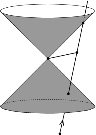
Figure 2: A timelike line $\ell=\{r+\lambda v\mid\lambda\in\mathbb{R}\}$ intersects the light-cone with vertex $p\not\in\ell$ in two points: $q_{+}$, its intersection with the future light-cone and $q_{-}$, its intersection with past the light cone. $q$ is a point inbetween $q_{+}$ and $q_{-}$.

Proposition 9.

Let $\ell$ and $\mathcal{L}_{p}$ as in Lemma 8 with $v$ timelike. Let $q_{+}$ and $q_{-}$ be the two intersection points of $\ell$ with $\mathcal{L}_{p}$ and $q\in\ell$ a point between them. Then

$$\|q-p\|_{g}^{2}=\|q_{+}-q\|_{g}\,\|q-q_{-}\|_{g}\,.$$ (104)

Moreover, $\|q_{+}-q\|_{g}=\|q-q_{-}\|_{g}$ iff $p-q$ is perpendicular to $v$.

Proof.

The vectors $(q_{+}-p)=(q-p)+(q_{+}-q)$ and $(q_{-}-p)=(q-p)+(q_{-}-q)$ are lightlike, which gives (note that $q-p$ is spacelike):

$$\|q-p\|_{g}^{2} \,=\,-(q-p)^{2} \,=\,(q_{+}-q)^{2}+2(q-p)\cdot(q_{+}-q)\,,$$ (105a)

$$\|q-p\|_{g}^{2} \,=\,-(q-p)^{2} \,=\,(q_{-}-q)^{2}+2(q-p)\cdot(q_{-}-q)\,.$$ (105b)

Since $q_{+}-q$ and $q-q_{-}$ are parallel we have $q_{+}-q=\lambda(q-q_{-})$ with $\lambda\in\mathbb{R}_{+}$ so that $(q_{+}-q)^{2}=\lambda\|q_{+}-q\|_{g}\|q-q_{-}\|_{g}$ and $\lambda(q_{-}-q)^{2}=\|q_{+}-q\|_{g}\|q-q_{-}\|_{g}$. Now, multiplying (105b) with $\lambda$ and adding this to (105a) immediately yields

$$(1+\lambda)\,\|q-p\|_{g}^{2}=(1+\lambda)\,\,\|q_{+}-q\|_{g}\|q-q_{-}\|_{g}\,.\\$$ (106)

Since $1+\lambda\neq 0$ this implies (104). Finally, since $q_{+}-q$ and $q_{-}-q$ are antiparallel, $\|q_{+}-q\|_{g}=\|q_{-}-q\|_{g}$ iff $(q_{+}-q)=-(q_{-}-q)$. Equations (105) now show that this is the case iff $(q-p)\cdot(q_{\pm}-q)=0$, i.e. iff $(q-p)\cdot v=0$. Hence we have shown

$$\|q_{+}-q\|_{g}=\|q-q_{-}\|_{g}\ \Longleftrightarrow\ (q-p)\cdot v=0\,.$$ (107)

In other words, $q$ is the midpoint of the segment $\overline{q_{+}q_{-}}$ iff the line through $p$ and $q$ is perpendicular (wrt. $g$) to $\ell$. ∎

The somewhat surprising feature of the first statement of this proposition is that (104) holds for any point of the segment $\overline{q_{+}q_{-}}$, not just the midpoint, as it would have to be the case for the corresponding statement in Euclidean geometry.

The second statement of Proposition 9 gives a convenient geometric characterization of Einstein-simultaneity. Recall that an event $q$ on a timelike line $\ell$ (representing an inertial observer) is defined to be Einstein-simultaneous with an event $p$ in spacetime iff $q$ bisects the segment $\overline{q_{+}q_{-}}$ between the intersection points $q_{+},q_{-}$ of $\ell$ with the double-lightcone at $p$. Hence Proposition 9 implies

Corollary 10.

Einstein simultaneity with respect to a timelike line $\ell$ is an equivalence relation on spacetime, the equivalence classes of which are the spacelike hyperplanes orthogonal (wrt. $g$) to $\ell$.

The first statement simply follows from the fact that the family of parallel hyperplanes orthogonal to $\ell$ form a partition (cf. Sect. A.1) of spacetime.

From now on we shall use the terms ‘timelike line’ and ‘inertial observer’ synonymously. Note that Einstein simultaneity is only defined relative to an inertial observer. Given two inertial observers,

$$\ell \,=\,\{r+\lambda v\mid\lambda\in\mathbb{R}\}\qquad \text{first observer}\,,$$ (108a)

$$\ell^{\prime} \,=\,\{r^{\prime}+\lambda^{\prime}v^{\prime}\mid\lambda^{\prime}\in\mathbb{R}\}\qquad \text{second observer}\,,$$ (108b)

we call the corresponding Einstein-simultaneity relations $\ell$-simultaneity and $\ell^{\prime}$-simultaneity. Obviously they coincide iff $\ell$ and $\ell^{\prime}$ are parallel ($v$ and $v^{\prime}$ are linearly dependent). In this case $q^{\prime}\in\ell^{\prime}$ is $\ell$-simultaneous to $q\in\ell$ iff $q\in\ell$ is $\ell^{\prime}$-simultaneous to $q^{\prime}\in\ell^{\prime}$. If $\ell$ and $\ell^{\prime}$are not parallel (skew or intersecting in one point) it is generally not true that if $q^{\prime}\in\ell^{\prime}$ is $\ell$-simultaneous to $q\in\ell$ then $q\in\ell$ is also $\ell^{\prime}$-simultaneous to $q^{\prime}\in\ell^{\prime}$. In fact, we have

Proposition 11.

Let $\ell$ and $\ell^{\prime}$ two non-parallel timelike likes. There exists a unique pair $(q,q^{\prime})\in\ell\times\ell^{\prime}$ so that $q^{\prime}$ is $\ell$-simultaneous to $q$ and $q$ is $\ell^{\prime}$ simultaneous to $q^{\prime}$.

Proof.

We parameterize $\ell$ and $\ell^{\prime}$ as in (108). The two conditions for $q^{\prime}$ being $\ell$-simultaneous to $q$ and $q$ being $\ell^{\prime}$-simultaneous to $q^{\prime}$ are $(q-q^{\prime})\cdot v=0=(q-q^{\prime})\cdot v^{\prime}$. Writing $q=r+\lambda v$ and $q^{\prime}=r^{\prime}+\lambda^{\prime}v^{\prime}$ this takes the form of the following matrix equation for the two unknowns $\lambda$ and $\lambda^{\prime}$:

$$\begin{pmatrix}v^{2}&-v\cdot v^{\prime}\\ v\cdot v^{\prime}&-v^{\prime 2}\end{pmatrix}\begin{pmatrix}\lambda\\ \lambda^{\prime}\end{pmatrix}=\begin{pmatrix}(r^{\prime}-r)\cdot v\\ (r^{\prime}-r)\cdot v^{\prime}\end{pmatrix}\,.$$ (109)

This has a unique solution pair $(\lambda,\lambda^{\prime})$, since for linearly independent timelike vectors $v$ and $v^{\prime}$ Lemma 7 implies $(v\cdot v^{\prime})^{2}-v^{2}v^{\prime 2}>0$. Note that if $\ell$ and $\ell^{\prime}$ intersect $q=q^{\prime}=\text{intersection point}$. ∎

Clearly, Einstein-simultaneity is conventional and physics proper should not depend on it. For example, the fringe-shift in the Michelson-Morley experiment is independent of how we choose to synchronize clocks. In fact, it does not even make use of any clock. So what is the general definition of a ‘simultaneity structure’? It seems obvious that it should be a relation on spacetime that is at least symmetric (each event should be simultaneous to itself). Going from one-way simultaneity to the mutual synchronization of two clocks, one might like to also require reflexivity (if $p$ is simultaneous to $q$ then $q$ is simultaneous to $p$), though this is not strictly required in order to one-way synchronize each clock in a set of clocks with one preferred ‘master clock’, which is sufficient for many applications.

Moreover, if we like to speak of the mutual simultaneity of sets of more than two events we need an equivalence relation on spacetime. The equivalence relation should be such that each inertial observer intersect each equivalence class precisely once. Let us call such a simultaneity structure ‘admissible’. Clearly there are zillions of such structures: just partition spacetime into any set of appropriate spacelike hypersurfaces (there are more possibilities at this point, like families of forward or backward lightcones). An absolute admissible simultaneity structure would be one which is invariant (cf. Sect. A.1) under the automorphism group of spacetime. We have

Proposition 12.

There exits precisely one admissible simultaneity structure which is invariant under the inhomogeneous proper orthochronous Galilei group and none that is invariant under the inhomogeneous proper orthochronous Lorentz group.

Proof.

See [25]. ∎

There is a group-theoretic reason that highlights this existential difference:

Proposition 13.

Let $G$ be a group with transitive action on a set $S$. Let $\mathrm{Stab}(p)\subset G$ be the stabilizer subgroup for $p\in S$ (due to transitivity all stabilizer subgroups are conjugate). Then $S$ admits a $G$-invariant equivalence relation $R\subset S\times S$ iff $\mathrm{Stab}(p)$ is not maximal, that is, iff $\mathrm{Stab}(p)$ is properly contained in a proper subgroup $H$ of $G$: $\mathrm{Stab}(p)\subsetneq H\subsetneq G$.

Proof.

See Theorem 1.12 in [33]. ∎

Regarding the action of the inhomogeneous Galilei and Lorentz groups on spacetime their stabilizers are the corresponding homogeneous groups. As already discussed at the end of Sect. 4.1, the homogeneous Lorentz group is maximal in the inhomogeneous one, whereas the homogeneous Galilei group is not maximal in the inhomogeneous one. This, according to Proposition 13, is the group theoretic origin of the absence of any invariant simultaneity structure in the Lorentzian case.

5.4 The lattice structure of causally and chronologically complete sets

Here we wish to briefly discuss another important structure associated with causality relations in Minkowski space, which plays a fundamental rôle in modern Quantum Field Theory (see e.g. [28]). Let $S_{1}$ and $S_{2}$ be subsets of $\mathbb{M}^{n}$. We say that $S_{1}$ and $S_{2}$ are causally disjoint or spacelike separated iff $p_{1}-p_{2}$ is spacelike, i.e. $(p_{1}-p_{2})^{2}<0$, for any $p_{1}\in S_{1}$ and $p_{2}\in S_{2}$. Note that because a point is not spacelike separated from itself, causally disjoint sets are necessarily disjoint in the ordinary set-theoretic sense—the converse being of course not true.

For any subset $S\subseteq\mathbb{M}^{n}$ we denote by $S^{\prime}$ the largest subset of $\mathbb{M}^{n}$ which is causally disjoint to $S$. The set $S^{\prime}$ is called the causal complement of $S$. The procedure of taking the causal complement can be iterated and we set $S^{\prime\prime}:=(S^{\prime})^{\prime}$ etc. $S^{\prime\prime}$ is called the causal completion of $S$. It also follows straight from the definition that $S_{1}\subseteq S_{2}$ implies $S^{\prime}_{1}\supseteq S^{\prime}_{2}$ and also $S^{\prime\prime}\supseteq S$. If $S^{\prime\prime}=S$ we call $S$ causally complete. We note that the causal complement $S^{\prime}$ of any given $S$ is automatically causally complete. Indeed, from $S^{\prime\prime}\supseteq S$ we obtain $(S^{\prime})^{\prime\prime}\subseteq S^{\prime}$, but the first inclusion applied to $S^{\prime}$ instead of $S$ leads to $(S^{\prime})^{\prime\prime}\supseteq S^{\prime}$, showing $(S^{\prime})^{\prime\prime}=S^{\prime}$. Note also that for any subset $S$ its causal completion, $S^{\prime\prime}$, is the smallest causally complete subset containing $S$, for if $S\subseteq K\subseteq S^{\prime\prime}$ with $K^{\prime\prime}=K$, we derive from the first inclusion by taking ^′′ that $S^{\prime\prime}\subseteq K$, so that the second inclusion yields $K=S^{\prime\prime}$. Trivial examples of causally complete subsets of $\mathbb{M}^{n}$ are the empty set, single points, and the total set $\mathbb{M}^{n}$. Others are the open diamond-shaped regions (99) as well as their closed counterparts:

$$\bar{U}(p,q):=(\mathcal{\bar{C}}^{+}_{p}\cap\mathcal{\bar{C}}^{-}_{q})\cup(\mathcal{\bar{C}}^{+}_{q}\cap\mathcal{\bar{C}}^{-}_{p})\,.$$ (110)

We now focus attention to the set $\mathrm{Caus}(\mathbb{M}^{n})$ of causally complete subsets of $\mathbb{M}^{n}$, including the empty set, $\emptyset$, and the total set, $\mathbb{M}^{n}$, which are mutually causally complementary. It is partially ordered by ordinary set-theoretic inclusion $(\subseteq)$ (cf. Sect. A.1) and carries the ‘dashing operation’ $(^{\prime})$ of taking the causal complement. Moreover, on $\mathrm{Caus}(\mathbb{M}^{n})$ we can define the operations of ‘meet’ and ‘join’, denoted by $\wedge$ and $\vee$ respectively, as follows: Let $S_{i}\in\mathrm{Caus}(\mathbb{M}^{n})$ where $i=1,2$, then $S_{1}\wedge S_{2}$ is the largest causally complete subset in the intersection $S_{1}\cap S_{2}$ and $S_{1}\vee S_{2}$ is the smallest causally complete set containing the union $S_{1}\cup S_{2}$.

The operations of $\wedge$ and $\vee$ can be characterized in terms of the ordinary set-theoretic intersection $\cap$ together with the dashing-operation. To see this, consider two causally complete sets, $S_{i}$ where $i=1,2$, and note that the set of points that are spacelike separated from $S_{1}$ and $S_{2}$ are obviously given by $S^{\prime}_{1}\cap S^{\prime}_{2}$, but also by $(S_{1}\cup S_{2})^{\prime}$, so that

$$S^{\prime}_{1}\cap S^{\prime}_{2} \,=\,(S_{1}\cup S_{2})^{\prime}\,,$$ (111a)

$$S_{1}\cap S_{2} \,=\,(S^{\prime}_{1}\cup S^{\prime}_{2})^{\prime}\,.$$ (111b)

Here (111a) and (111b) are equivalent since any $S_{i}\in\mathrm{Caus}(\mathbb{M}^{n})$ can be written as $S_{i}=P^{\prime}_{i}$, namely $P_{i}=S^{\prime}_{i}$. If $S_{i}$ runs through all sets in $\mathrm{Caus}(\mathbb{M}^{n})$ so does $P_{i}$. Hence any equation that holds generally for all $S_{i}\in\mathrm{Caus}(\mathbb{M}^{n})$ remains valid if the $S_{i}$ are replaced by $S^{\prime}_{i}$.

Equation (111b) immediately shows that $S_{1}\cap S_{2}$ is causally complete (since it is the ^′ of something). Taking the causal complement of (111a) we obtain the desired relation for $S_{1}\vee S_{2}:=(S_{1}\cup S_{2})^{\prime\prime}$. Together we have

$$S_{1}\wedge S_{2} \,=\,S_{1}\cap S_{2}\,,$$ (112a)

$$S_{1}\vee S_{2} \,=\,(S^{\prime}_{1}\cap S^{\prime}_{2})^{\prime}\,.$$ (112b)

From these we immediately derive

$$(S_{1}\wedge S_{2})^{\prime} \,=\,S^{\prime}_{1}\vee S^{\prime}_{2}\,,$$ (113a)

$$(S_{1}\vee S_{2})^{\prime} \,=\,S^{\prime}_{1}\wedge S^{\prime}_{2}\,.$$ (113b)

All what we have said so far for the set $\mathrm{Caus}(\mathbb{M}^{n})$ could be repeated verbatim for the set $\mathrm{Chron}(\mathbb{M}^{n})$ of chronologically complete subsets. We say that $S_{1}$ and $S_{2}$ are chronologically disjoint or non-timelike separated, iff $S_{1}\cap S_{2}=\emptyset$ and $(p_{1}-p_{2})^{2}\leq 0$ for any $p_{1}\in S_{1}$ and $p_{2}\in S_{2}$. $S^{\prime}$, the chronological complement of $S$, is now the largest subset of $\mathbb{M}^{n}$ which is chronologically disjoint to $S$. The only difference between the causal and the chronological complement of $S$ is that the latter now contains lightlike separated points outside $S$. A set $S$ is chronologically complete iff $S=S^{\prime\prime}$, where the dashing now denotes the operation of taking the chronological complement. Again, for any set $S$ the set $S^{\prime}$ is automatically chronologically complete and $S^{\prime\prime}$ is the smallest chronologically complete subset containing $S$. Single points are chronologically complete subsets. All the formal properties regarding ^′, $\wedge$, and $\vee$ stated hitherto for $\mathrm{Caus}(\mathbb{M}^{n})$ are the same for $\mathrm{Chron}(\mathbb{M}^{n})$.

One major difference between $\mathrm{Caus}(\mathbb{M}^{n})$ and $\mathrm{Chron}(\mathbb{M}^{n})$ is that the types of diamond-shaped sets they contain are different. For example, the closed ones, (110), are members of both. The open ones, (99), are contained in $\mathrm{Caus}(\mathbb{M}^{n})$ but not in $\mathrm{Chron}(\mathbb{M}^{n})$. Instead, $\mathrm{Chron}(\mathbb{M}^{n})$ contains the closed diamonds whose ‘equator’ have been removed. An essential structural difference between $\mathrm{Caus}(\mathbb{M}^{n})$ and $\mathrm{Chron}(\mathbb{M}^{n})$ will be stated below, after we have introduced the notion of a lattice to which we now turn.

To put all these formal properties into the right frame we recall the definition of a lattice. Let $(L,\leq)$ be a partially ordered set and $a,b$ any two elements in $L$. Synonymously with $a\leq b$ we also write $b\geq a$ and say that $a$ is smaller than $b$, $b$ is bigger than $a$, or $b$ majorizes $a$. We also write $a<b$ if $a\leq b$ and $a\neq b$. If, with respect to $\leq$, their greatest lower and least upper bound exist, they are denoted by $a\wedge b$—called the ‘meet of $a$ and $b$’—and $a\vee b$—called the ‘join of $a$ and $b$’—respectively. A partially ordered set for which the greatest lower and least upper bound exist for any pair $a,b$ of elements from $L$ is called a lattice.

We now list some of the most relevant additional structural elements lattices can have: A lattice is called complete if greatest lower and least upper bound exist for any subset $K\subseteq L$. If $K=L$ they are called $0$ (the smallest element in the lattice) and $1$ (the biggest element in the lattice) respectively. An atom in a lattice is an element $a$ which majorizes only $0$, i.e. $0\leq a$ and if $0\leq b\leq a$ then $b=0$ or $b=a$. The lattice is called atomic if each of its elements different from $0$ majorizes an atom. An atomic lattice is called atomistic if every element is the join of the atoms it majorizes. An element $c$ is said to cover $a$ if $a<c$ and if $a\leq b\leq c$ either $a=b$ or $b=c$. An atomic lattice is said to have the covering property if, for every element $b$ and every atom $a$ for which $a\wedge b=0$, the join $a\vee b$ covers $b$.

The subset $\{a,b,c\}\subseteq L$ is called a distributive triple if

$$a\wedge(b\vee c) \,=\,(a\wedge b)\vee(a\wedge c)\quad \text{and $(a,b,c)$ cyclically permuted}\,,$$ (114a)

$$a\vee(b\wedge c) \,=\,(a\vee b)\wedge(a\vee c)\quad \text{and $(a,b,c)$ cyclically permuted}\,.$$ (114b)

Definition 5.

A lattice is called distributive or Boolean if every triple $\{a,b,c\}$ is distributive. It is called modular if every triple $\{a,b,c\}$ with $a\leq b$ is distributive.

It is straightforward to check from (114) that modularity is equivalent to the following single condition:

$$\text{modularity}\Leftrightarrow a\vee(b\wedge c)=b\wedge(a\vee c)\quad\text{for all $a,b,c\in L$ s.t. $a\leq b$.}$$ (115)

If in a lattice with smallest element $0$ and greatest element $1$ a map $L\rightarrow L$, $a\mapsto a^{\prime}$, exist such that

$$a^{\prime\prime}:=(a^{\prime})^{\prime}=a\,,$$ (116a)

$$a\leq b\Rightarrow b^{\prime}\leq a^{\prime}\,,$$ (116b)

$$a\wedge a^{\prime}=0\,,\quad a\vee a^{\prime}=1\,,$$ (116c)

the lattice is called orthocomplemented. It follows that whenever the meet and join of a subset $\{a_{i}\mid i\in I\}$ ($I$ is some index set) exist one has De Morgan’s laws:

$$\bigl{(}\textstyle{\bigwedge_{i\in I}}\ a_{i}\bigr{)}^{\prime} \,=\,\textstyle{\bigvee_{i\in I}}\ a^{\prime}_{i}\,,$$ (117a)

$$\bigl{(}\textstyle{\bigvee_{i\in I}}\ a_{i}\bigr{)}^{\prime} \,=\,\textstyle{\bigwedge_{i\in I}}\ a^{\prime}_{i}\,.$$ (117b)

For orthocomplemented lattices there is a still weaker version of distributivity than modularity, which turns out to be physically relevant in various contexts:

Definition 6.

An orthocomplemented lattice is called orthomodular if every triple $\{a,b,c\}$ with $a\leq b$ and $c\leq b^{\prime}$ is distributive.

From (115) and using that $b\wedge c=0$ for $b\leq c^{\prime}$ one sees that this is equivalent to the single condition (renaming $c$ to $c^{\prime}$):

orthomod. $$\Leftrightarrow\quad a\,=\,b\wedge(a\vee c^{\prime})\quad a,b,c\in L a\leq b\leq c$$ for all s.t.  , (118a)

$$\Leftrightarrow a\,=\,b\vee(a\wedge c^{\prime})\quad a,b,c\in L a\geq b\geq c$$ for all s.t.  , (118b)

where the second line follows from the first by taking its orthocomplement and renaming $a^{\prime},b^{\prime},c$ to $a,b,c^{\prime}$. It turns out that these conditions can still be simplified by making them independent of $c$. In fact, (118) are equivalent to

orthomod. $$\Leftrightarrow\quad a=b\wedge(a\vee b^{\prime})\quad a,b\in L a\leq b$$ for all s.t.  , (119a)

$$\Leftrightarrow a=b\vee(a\wedge b^{\prime})\quad a,b\in L a\geq b$$ for all s.t.  . (119b)

It is obvious that (118) implies (119) (set $c=b$). But the converse is also true. To see this, take e.g. (119b) and choose any $c\leq b$. Then $c^{\prime}\geq b^{\prime}$, $a\geq b$ (by hypothesis), and $a\geq a\wedge c^{\prime}$ (trivially), so that $a\geq b\vee(a\wedge c^{\prime})$. Hence $a\geq b\vee(a\wedge c^{\prime})\geq b\vee(a\wedge b^{\prime})=a$, which proves (118b).

Complete orthomodular atomic lattices are automatically atomistic. Indeed, let $b$ be the join of all atoms majorized by $a\neq 0$. Assume $a\neq b$ so that necessarily $b<a$, then (119b) implies $a\wedge b^{\prime}\neq 0$. Then there exists an atom $c$ majorized by $a\wedge b^{\prime}$. This implies $c\leq a$ and $c\leq b^{\prime}$, hence also $c\not\leq b$. But this is a contradiction, since $b$ is by definition the join of all atoms majorized by $a$.

Finally we mention the notion of compatibility or commutativity, which is a symmetric, reflexive, but generally not transitive relation $R$ on an orthomodular lattice (cf. Sec. A.1). We write $a\natural b$ for $(a,b)\in R$ and define:

$$a\natural b\quad \Leftrightarrow\quad a \,=\,(a\wedge b)\vee(a\wedge b^{\prime})\,,$$ (120a)

$$\Leftrightarrow\quad b \,=\,(b\wedge a)\vee(b\wedge a^{\prime})\,.$$ (120b)

The equivalence of these two lines, which shows that the relation of being compatible is indeed symmetric, can be demonstrated using orthomodularity as follows: Suppose (120a) holds; then $b\wedge a^{\prime}=b\wedge(b^{\prime}\vee a^{\prime})\wedge(b\vee a^{\prime})=b\wedge(b^{\prime}\vee a^{\prime})$, where we used the orthocomplement of (120a) to replace $a^{\prime}$ in the first expression and the trivial identity $b\wedge(b\vee a^{\prime})=b$ in the second step. Now, applying (119b) to $b\geq a\wedge b$ we get $b=(b\wedge a)\vee[b\wedge(b^{\prime}\vee a^{\prime})]=(b\wedge a)\vee(b\wedge a^{\prime})$, i.e. (120b). The converse, $(\ref{eq:DefCompatibility2})\Rightarrow(\ref{eq:DefCompatibility1})$, is of course entirely analogous.

From (120) a few things are immediate: $a\natural b$ is equivalent to $a\natural b^{\prime}$, $a\natural b$ is implied by $a\leq b$ or $a\leq b^{\prime}$, and the elements $0$ and $1$ are compatible with all elements in the lattice. The center of a lattice is the set of elements which are compatible with all elements in the lattice. In fact, the center is a Boolean sublattice. If the center contains no other elements than $0$ and $1$ the lattice is said to be irreducible. The other extreme is a Boolean lattice, which is identical to its own center. Indeed, if $(a,b,b^{\prime})$ is a distributive triple, one has $a=a\wedge 1=a\wedge(b\vee b^{\prime})=(a\wedge b)\vee(a\wedge b^{\prime})\Rightarrow(\ref{eq:DefCompatibility1})$.

After these digression into elementary notions of lattice theory we come back to our examples of the sets $\mathrm{Caus}(\mathbb{M}^{n})$ $\mathrm{Chron}(\mathbb{M}^{n})$. Our statements above amount to saying that they are complete, atomic, and orthocomplemented lattices. The partial order relation $\leq$ is given by $\subseteq$ and the extreme elements $0$ and $1$ correspond to the empty set $\emptyset$ and the total set $\mathbb{M}^{n}$, the points of which are the atoms. Neither the covering property nor modularity is shared by any of the two lattices, as can be checked by way of elementary counterexamples. In particular, neither of them is Boolean. However, in [15] it was shown that $\mathrm{Chron}(\mathbb{M}^{n})$ is orthomodular; see also [13] which deals with more general spacetimes. Note that by the argument given above this implies that $\mathrm{Chron}(\mathbb{M}^{n})$ is atomistic. In contrast, $\mathrm{Caus}(\mathbb{M}^{n})$ is definitely not orthomodular, as is e.g. seen by the counterexample given in Fig. 3. It is also not difficult to prove that $\mathrm{Chron}(\mathbb{M}^{n})$ is irreducible.

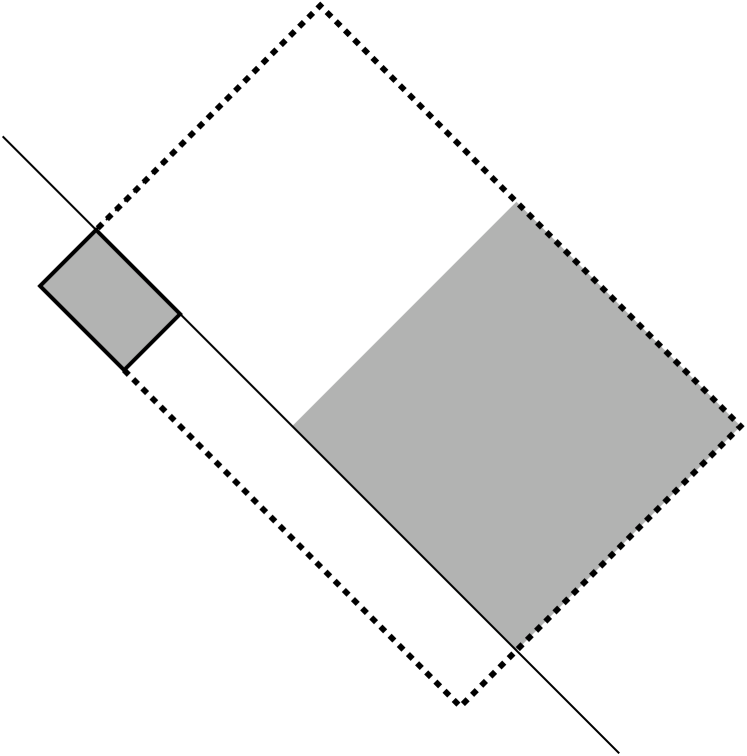
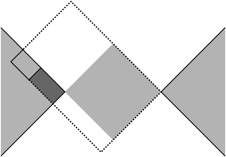
Figure 3: The two figures show that $\text{Caus}(\mathbb{M}^{n})$ is not orthomodular. The first thing to note is that $\text{Caus}(\mathbb{M}^{n})$ contains open (99) as well as closed (110) diamond sets. In the left picture we consider the join of a small closed diamond $a$ with a large open diamond $b^{\prime}$. (Closed sets are indicated by a solid boundary line.) Their edges are aligned along the lightlike line $\ell$. Even though these regions are causally disjoint, their causal completion is much larger than their union and given by the open (for $n>2$) enveloping diamond $a\vee b^{\prime}$ framed by the dashed line. (This also shows that the join of two regions can be larger than the domain of dependence of their union; compare footnote 24.) . Next we consider the situation depicted on the right side. The closed double-wedge region $b$ contains the small closed diamond $a$. The causal complement $b^{\prime}$ of $b$ is the open diamond in the middle. $a\vee b^{\prime}$ is, according to the first picture, given by the large open diamond enclosed by the dashed line. The intersection of $a\vee b^{\prime}$ with $b$ is strictly larger than $a$, the difference being the dark-shaded region in the left wedge of $b$ below $a$. Hence $a\neq b\wedge(a\vee b^{\prime})$, in contradiction to (119a).

It is well known that the lattices of propositions for classical systems are Boolean, whereas those for quantum systems are merely orthomodular. In classical physics the elements of the lattice are measurable subsets of phase space, with $\leq$ being ordinary set-theoretic inclusion $\subseteq$, and $\wedge$ and $\vee$ being ordinary set-theoretic intersection $\cap$ and union $\cup$ respectively. The orthocomplement is the ordinary set-theoretic complement. In Quantum Mechanics the elements of the lattice are the closed subspaces of Hilbert space, with $\leq$ being again ordinary inclusion, $\wedge$ ordinary intersection, and $\vee$ is given by $a\vee b:=\overline{\mbox{span}\{a,b\}}$. The orthocomplement of a closed subset is the orthogonal complement in Hilbert space. For comprehensive discussions see [34] and [5].

One of the main questions in the foundations of Quantum Mechanics is whether one could understand (derive) the usage of Hilbert spaces and complex numbers from somehow more fundamental principles. Even though it is not a priori clear what ones measure of fundamentality should be at this point, an interesting line of attack consists in deriving the mentioned structures from the properties of the lattice of propositions (Quantum Logic). It can be shown that a lattice that is complete, atomic, irreducible, orthomodular, and that satisfies the covering property is isomorphic to the lattice of closed subspaces of a linear space with Hermitean inner product. The complex numbers are selected if additional technical assumptions are added. For the precise statements of these reconstruction theorems see [5].

It is now interesting to note that, on a formal level, there is a similar transition in going from Galilei invariant to Lorentz invariant causality relations. In fact, in Galilean spacetime one can also define a chronological complement: Two points are chronologically related if they are connected by a worldline of finite speed and, accordingly, two subsets in spacetime are chronologically disjoint if no point in one set is chronologically related to a point of the other. For example, the chronological complement of a point $p$ are all points simultaneous to, but different from, $p$. More general, it is not hard to see that the chronologically complete sets are just the subsets of some $t=\text{const.}$ hypersurface. The lattice of chronologically complete sets is then the continuous disjoint union of sublattices, each of which is isomorphic to the Boolean lattice of subsets in $\mathbb{R}^{3}$. For details see [14].

As we have seen above, $\text{Chron}(\mathbb{M}^{n})$ is complete, atomic, irreducible, and orthomodular (hence atomistic). The main difference to the lattice of propositions in Quantum Mechanics, as regards the formal aspects discussed here, is that $\text{Chron}(\mathbb{M}^{n})$ does not satisfy the covering property. Otherwise the formal similarities are intriguing and it is tempting to ask whether there is a deeper meaning to this. In this respect it would be interesting to know whether one could give a lattice-theoretic characterization for $\text{Chron}(M)$ ($M$ some fixed spacetime), comparable to the characterization of the lattices of closed subspaces in Hilbert space alluded to above. Even for $M=\mathbb{M}^{n}$ such a characterization seems, as far as I am aware, not to be known.

5.5 Rigid motion

As is well known, the notion of a rigid body, which proves so useful in Newtonian mechanics, is incompatible with the existence of a universal finite upper bound for all signal velocities [37]. As a result, the notion of a perfectly rigid body does not exist within the framework of SR. However, the notion of a rigid motion does exist. Intuitively speaking, a body moves rigidly if, locally, the relative spatial distances of its material constituents are unchanging.

The motion of an extended body is described by a normalized timelike vector field $u:\Omega\rightarrow\mathbb{R}^{n}$, where $\Omega$ is an open subset of Minkowski space, consisting of the events where the material body in question ‘exists’. We write $g(u,u)=u\cdot u=u^{2}$ for the Minkowskian scalar product. Being normalized now means that $u^{2}=c^{2}$ (we do not choose units such that $c=1$). The Lie derivative with respect to $u$ is denoted by $L_{u}$.

For each material part of the body in motion its local rest space at the event $p\in\Omega$ can be identified with the hyperplane through $p$ orthogonal to $u_{p}$:

$$H_{p}:=p+u_{p}^{\perp}\,.$$ (121)

$u_{p}^{\perp}$ carries a Euclidean inner product, $h_{p}$, given by the restriction of $-g$ to $u_{p}^{\perp}$. Generally we can write

$$h=c^{-2}\,u^{\flat}\otimes u^{\flat}-g\,,$$ (122)

where $u^{\flat}=g^{\downarrow}(u):=g(u,\cdot)$ is the one-form associated (‘index-lowered’, cf. Sec. A.5) to $u$. Following [12] the precise definition of ‘rigid motion’ can now be given as follows:

Definition 7 (Born 1909).

Let $u$ be a normalized timelike vector field $u$. The motion described by its flow is rigid if

$$L_{u}h=0\,.$$ (123)

Note that, in contrast to the Killing equations $L_{u}g=0$, these equations are non linear due to the dependence of $h$ upon $u$.

We write $\Pi_{h}:=\text{id}-c^{-2}\,u\otimes u^{\flat}\in\mbox{End}(\mathbb{R}^{n})$ for the tensor field over spacetime that pointwise projects vectors perpendicular to $u$. It acts on one forms $\alpha$ via $\Pi_{h}(\alpha):=\alpha\circ\Pi_{h}$ and accordingly on all tensors. The so extended projection map will still be denoted by $\Pi_{h}$. Then we e.g. have

$$h=-\Pi_{h}g:=-g(\Pi_{h}\cdot,\Pi_{h}\cdot)\,.$$ (124)

It is not difficult to derive the following two equations:

$$L_{fu}h \,=\,fL_{u}h\,,$$ (125)

$$L_{u}h \,=\,-L_{u}(\Pi_{h}g)=-\Pi_{h}(L_{u}g)\,,$$ (126)

where $f$ is any differentiable real-valued function on $\Omega$.

Equation (125) shows that the normalized vector field $u$ satisfies (123) iff any rescaling $fu$ with a nowhere vanishing function $f$ does. Hence the normalization condition for $u$ in (123) is really irrelevant. It is the geometry in spacetime of the flow lines and not their parameterization which decide on whether motions (all, i.e. for any parameterization, or none) along them are rigid. This has be the case because, generally speaking, there is no distinguished family of sections (hypersurfaces) across the bundle of flow lines that would represent ‘the body in space’, i.e. mutually simultaneous locations of the body’s points. Distinguished cases are those exceptional ones in which $u$ is hypersurface orthogonal. Then the intersection of $u$’s flow lines with the orthogonal hypersurfaces consist of mutually Einstein synchronous locations of the points of the body. An example is discussed below.

Equation (126) shows that the rigidity condition is equivalent to the ‘spatially’ projected Killing equation. We call the flow of the timelike normalized vector field $u$ a Killing motion (i.e. a spacetime isometry) if there is a Killing field $K$ such that $u=cK/\sqrt{K^{2}}$. Equation (126) immediately implies that Killing motions are rigid. What about the converse? Are there rigid motions that are not Killing? This turns out to be a difficult question. Its answer in Minkowski space is: ‘yes, many, but not as many as naively expected.’

Before we explain this, let us give an illustrative example for a Killing motion, namely that generated by the boost Killing-field in Minkowski space. We suppress all but one spatial directions and consider boosts in $x$ direction in two-dimensional Minkowski space (coordinates $ct$ and $x$; metric $ds^{2}=c^{2}dt^{2}-dx^{2}$). The Killing field is

$$K=x\,\partial_{ct}+ct\,\partial_{x}\,,$$ (127)

which is timelike in the region $|x|>|ct|$. We focus on the ‘right wedge’ $x>|ct|$, which is now our region $\Omega$. Consider a rod of length $\ell$ which at $t=0$ is represented by the interval $x\in(r,r+\ell)$, where $r>0$. The flow of the normalized field $u=cK/\sqrt{K^{2}}$ is

$$ct(\tau) \,=\,x_{0}\,\sinh\bigl{(}c\tau/x_{0})\,,$$ (128a)

$$x(\tau) \,=\,x_{0}\,\cosh\bigl{(}c\tau/x_{0})\,,$$ (128b)

where $x_{0}=x(\tau=0)\in(r,r+\ell)$ labels the elements of the rod at $\tau=0$. We have $x^{2}-c^{2}t^{2}=x_{0}^{2}$, showing that the individual elements of the rod move on hyperbolae (‘hyperbolic motion’). $\tau$ is the proper time along each orbit, normalized so that the rod lies on the $x$ axis at $\tau=0$.

The combination

$$\lambda:=c\tau/x_{0}$$ (129)

is just the flow parameter for $K$ (127), sometimes referred to as ‘Killing time’ (though it is dimensionless). From (128) we can solve for $\lambda$ and $\tau$ as functions of $ct$ and $x$:

$$\lambda \,=\,f(ct,x) \,:=\,\tanh^{-1}\bigl{(}ct/x\bigr{)}\,,$$ (130a)

$$\tau \,=\,\hat{f}(ct,x) \,:=\,\underbrace{\sqrt{(x/c)^{2}-t^{2}}}_{x_{0}/c}\,\tanh^{-1}\bigl{(}ct/x\bigr{)}\,,$$ (130b)

from which we infer that the hypersurfaces of constant $\lambda$ are hyperplanes which all intersect at the origin. Moreover, we also have $df=K^{\flat}/K^{2}$ ($d$ is just the ordinary exterior differential) so that the hyperplanes of constant $\lambda$ intersect all orbits of $u$ (and $K$) orthogonally. Hence the hyperplanes of constant $\lambda$ qualify as the equivalence classes of mutually Einstein-simultaneous events in the region $x>|ct|$ for a family of observers moving along the Killing orbits. This does not hold for the hypersurfaces of constant $\tau$, which are curved.

The modulus of the spacetime-acceleration (which is the same as the modulus of the spatial acceleration measured in the local rest frame) of the material part of the rod labeled by $x_{0}$ is

$$\|a\|_{g}=c^{2}/x_{0}\,.$$ (131)

As an aside we generally infer from this that, given a timelike curve of local acceleration (modulus) $\alpha$, infinitesimally nearby orthogonal hyperplanes intersect at a spatial distance $c^{2}/\alpha$. This remark will become relevant in the discussion of part 2 of the Noether-Herglotz theorem given below.

In order to accelerate the rod to the uniform velocity $v$ without deforming it, its material point labeled by $x_{0}$ has to accelerate for the eigentime (this follows from (128))

$$\tau=\frac{x_{0}}{c}\tanh^{-1}(v/c)\,,$$ (132)

which depends on $x_{0}$. In contrast, the Killing time is the same for all material points and just given by the final rapidity. In particular, judged from the local observers moving with the rod, a rigid acceleration requires accelerating the rod’s trailing end harder but shorter than pulling its leading end.

In terms of the coordinates $(\lambda,x_{0})$, which are comoving with the flow of $K$, and $(\tau,x_{0})$, which are comoving with the flow of $u$, we just have $K=\partial/\partial\lambda$ and $u=\partial/\partial\tau$ respectively. The spacetime metric $g$ and the projected metric $h$ in terms of these coordinates are:

$$h \,=\,dx_{0}^{2}\,,$$ (133a)

$$g \,=\,x_{0}^{2}\,d\lambda^{2}-dx_{0}^{2}=c^{2}\bigl{(}d\tau-(\tau/x_{0})\,dx_{0}\bigr{)}^{2}-dx_{0}^{2}\,.$$ (133b)

Note the simple form $g$ takes in terms of $x_{0}$ and $\lambda$, which are also called the ‘Rindler coordinates’ for the region $|x|>|ct|$ of Minkowski space. They are the analogs in Lorentzian geometry to polar coordinates (radius $x_{0}$, angle $\lambda$) in Euclidean geometry.

Let us now return to the general case. We decompose the derivative of the velocity one-form $u^{\flat}:=g^{\downarrow}(u)$ as follows:

$$\nabla u^{\flat}=\theta+\omega+c^{-2}\,u^{\flat}\otimes a^{\flat}\,,$$ (134)

where $\theta$ and $\omega$ are the projected symmetrized and antisymmetrized derivatives respectively

$$2\theta \,=\,\Pi_{h}(\nabla\vee u^{\flat}) \,=\,\nabla\vee u^{\flat}-c^{-2}\,u^{\flat}\vee a^{\flat}\,,$$ (135a)

$$2\omega \,=\,\Pi_{h}(\nabla\wedge u^{\flat}) \,=\,\nabla\wedge u^{\flat}-c^{-2}\,u^{\flat}\wedge a^{\flat}\,.$$ (135b)

The symmetric part, $\theta$, is usually further decomposed into its traceless and pure trace part, called the shear and expansion of $u$ respectively. The antisymmetric part $\omega$ is called the vorticity of $u$.

Now recall that the Lie derivative of $g$ is just twice the symmetrized derivative, which in our notation reads:

$$L_{u}g=\nabla\vee u^{\flat}\,.$$ (136)

This implies in view of (123), (126), and (135a)

Proposition 14.

Let $u$ be a normalized timelike vector field $u$. The motion described by its flow is rigid iff $u$ is of vanishing shear and expansion, i.e. iff $\theta=0$.

Vector fields generating rigid motions are now classified according to whether or not they have a vanishing vorticity $\omega$: if $\omega=0$ the flow is called irrotational, otherwise rotational. The following theorem is due to Herglotz [30] and Noether [38]:

Theorem 15 (Noether & Herglotz, part 1).

A rotational rigid motion in Minkowski space must be a Killing motion.

An example of such a rotational motion is given by the Killing field

$$K=\partial_{t}+\kappa\,\partial_{\varphi}$$ (137)

inside the region

$$\Omega=\{(t,z,\rho,\varphi)\mid\kappa\rho<c\}\,,$$ (138)

where $K$ is timelike. This motion corresponds to a rigid rotation with constant angular velocity $\kappa$ which, without loss of generality, we take to be positive. Using the comoving angular coordinate $\psi:=\varphi-\kappa t$, the split (122) is now furnished by

$$u^{\flat} \,=\,c\,\sqrt{1-(\kappa\rho/c)^{2}}\left\{c\,dt-\frac{\kappa\rho/c}{1-(\kappa\rho/c)^{2}}\ \rho\,d\psi\right\}\,,$$ (139a)

$$h \,=\,dz^{2}+d\rho^{2}+\frac{\rho^{2}\,d\psi^{2}}{1-(\kappa\rho/c)^{2}}\,.$$ (139b)

The metric $h$ is curved (cf. Lemma 16). But the rigidity condition (123) means that $h$, and hence its curvature, cannot change along the motion. Therefore, even though we can keep a body in uniform rigid rotational motion, we cannot put it into this state from rest by purely rigid motions, since this would imply a transition from a flat to a curved geometry of the body. This was first pointed out by Ehrenfest [17]. Below we will give a concise analytical expression of this fact (cf. equation (143)). All this is in contrast to the translational motion, as we will also see below.

The proof of Theorem 15 relies on arguments from differential geometry proper and is somewhat tricky. Here we present the essential steps, basically following [39] and [45] in a slightly modernized notation. Some straightforward calculational details will be skipped. The argument itself is best broken down into several lemmas.

At the heart of the proof lies the following general construction: Let $M$ be the spacetime manifold with metric $g$ and $\Omega\subset M$ the open region in which the normalized vector field $u$ is defined. We take $\Omega$ to be simply connected. The orbits of $u$ foliate $\Omega$ and hence define an equivalence relation on $\Omega$ given by $p\sim q$ iff $p$ and $q$ lie on the same orbit. The quotient space $\hat{\Omega}:=\Omega/\!\!\sim$ is itself a manifold. Tensor fields on $\hat{\Omega}$ can be represented by (i.e. are in bijective correspondence to) tensor fields $T$ on $\Omega$ which obey the two conditions:

$$\Pi_{h}\,T \,=\,T\,,$$ (140a)

$$L_{u}T \,=\,0\,.$$ (140b)

Tensor fields satisfying (140a) are called horizontal, those satisfying both conditions (140) are called projectable. The $(n-1)$-dimensional metric tensor $h$, defined in (122), is an example of a projectable tensor if $u$ generates a rigid motion, as assumed here. It turns $(\hat{\Omega},h)$ into a $(n-1)$-dimensional Riemannian manifold. The covariant derivative $\hat{\nabla}$ with respect to the Levi-Civita connection of $h$ is given by the following operation on projectable tensor fields:

$$\hat{\nabla}:=\Pi_{h}\circ\nabla$$ (141)

i.e. by first taking the covariant derivative $\nabla$ (Levi-Civita connection in $(M,g)$) in spacetime and then projecting the result horizontally. This results again in a projectable tensor, as a straightforward calculation shows.

The horizontal projection of the spacetime curvature tensor can now be related to the curvature tensor of $\hat{\Omega}$ (which is a projectable tensor field). Without proof we state

Lemma 16.

Let $u$ generate a rigid motion in spacetime. Then the horizontal projection of the totally covariant (i.e. all indices down) curvature tensor $R$ of $(\Omega,g)$ is related to the totally covariant curvature tensor $\hat{R}$ of $(\hat{\Omega},h)$ by the following equation:

$$\Pi_{h}R=-\hat{R}-3\,(\text{\rm id}-\Pi_{\wedge})\omega\otimes\omega\,,$$ (142)

where $\Pi_{\wedge}$ is the total antisymmetrizer, which here projects tensors of rank four onto their totally antisymmetric part.

Formula (142) is true in any spacetime dimension $n$. Note that the projector $(\text{id}-\Pi_{\wedge})$ guarantees consistency with the first Bianchi identities for $R$ and $\hat{R}$, which state that the total antisymmetrization in their last three slots vanish identically. This is consistent with (142) since for tensors of rank four with the symmetries of $\omega\otimes\omega$ the total antisymmetrization on tree slots is identical to $\Pi_{\wedge}$, the symmetrization on all four slots. The claim now simply follows from $\Pi_{\wedge}\circ(\text{id}-\Pi_{\wedge})=\Pi_{\wedge}-\Pi_{\wedge}=0$.

We now restrict to spacetime dimensions of four or less, i.e. $n\leq 4$. In this case $\Pi_{\wedge}\circ\Pi_{h}=0$ since $\Pi_{h}$ makes the tensor effectively live over $n-1$ dimensions, and any totally antisymmetric four-tensor in three or less dimensions must vanish. Applied to (142) this means that $\Pi_{\wedge}(\omega\otimes\omega)=0$, for horizontality of $\omega$ implies $\omega\otimes\omega=\Pi_{h}(\omega\otimes\omega)$. Hence the right hand side of (142) just contains the pure tensor product $-3\,\omega\otimes\omega$.

Now, in our case $R=0$ since $(M,g)$ is flat Minkowski space. This has two interesting consequences: First, $(\hat{\Omega},h)$ is curved iff the motion is rotational, as exemplified above. Second, since $\hat{R}$ is projectable, its Lie derivative with respect to $u$ vanishes. Hence (142) implies $L_{u}\omega\otimes\omega+\omega\otimes L_{u}\omega=0$, which is equivalent to

$$L_{u}\omega=0\,.$$ (143)

This says that the vorticity cannot change along a rigid motion in flat space. It is the precise expression for the remark above that you cannot rigidly set a disk into rotation. Note that it also provides the justification for the global classification of rigid motions into rotational and irrotational ones.

A sharp and useful criterion for whether a rigid motion is Killing or not is given by the following

Lemma 17.

Let $u$ be a normalized timelike vector field on a region $\Omega\subseteq M$. The motion generated by $u$ is Killing iff it is rigid and $a^{\flat}$ is exact on $\Omega$.

Proof.

That the motion generated by $u$ be Killing is equivalent to the existence of a positive function $f:\Omega\rightarrow\mathbb{R}$ such that $L_{fu}g=0$, i.e. $\nabla\vee(fu^{\flat})=0$. In view of (135a) this is equivalent to

$$2\theta+(d\ln f+c^{-2}a^{\flat})\vee u^{\flat}=0\,,$$ (144)

which, in turn, is equivalent to $\theta=0$ and $a^{\flat}=-c^{2}\,d\ln f$. This is true since $\theta$ is horizontal, $\Pi_{h}\theta=\theta$, whereas the first term in (144) vanishes upon applying $\Pi_{h}$. The result now follows from reading this equivalence both ways: 1) The Killing condition for $K:=fu$ implies rigidity for $u$ and exactness of $a^{\flat}$. 2) Rigidity of $u$ and $a^{\flat}=-d\Phi$ imply that $K:=fu$ is Killing, where $f:=\exp(\Phi/c^{2})$. ∎

We now return to the condition (143) and express $L_{u}\omega$ in terms of $du^{\flat}$. For this we recall that $L_{u}u^{\flat}=a^{\flat}$ (cf. footnote 26) and that Lie derivatives on forms commute with exterior derivatives. Hence we have

$$2\,L_{u}\omega=L_{u}(\Pi_{h}du^{\flat})=\Pi_{h}da^{\flat}=da^{\flat}-c^{-2}u^{\flat}\wedge L_{u}a^{\flat}\,.$$ (145)

Here we used the fact that the additional terms that result from the Lie derivative of the projection tensor $\Pi_{h}$ vanish, as a short calculation shows, and also that on forms the projection tensor $\Pi_{h}$ can be written as $\Pi_{h}=\text{id}-c^{-2}u^{\flat}\wedge i_{u}$, where $i_{u}$ denotes the map of insertion of $u$ in the first slot.

Now we prove

Lemma 18.

Let $u$ generate a rigid motion in flat space such that $\omega\neq 0$, then

$$L_{u}a^{\flat}=0\,.$$ (146)

Proof.

Equation (143) says that $\omega$ is projectable (it is horizontal by definition). Hence $\hat{\nabla}\omega$ is projectable, which implies

$$L_{u}\hat{\nabla}\omega=0\,.$$ (147)

Using (134) with $\theta=0$ one has

$$\hat{\nabla}\omega=\Pi_{h}\nabla\omega=\Pi_{h}\nabla\nabla u^{\flat}-c^{-2}\Pi_{h}(\nabla u^{\flat}\otimes a^{\flat})\,.$$ (148)

Antisymmetrization in the first two tensor slots makes the first term on the right vanish due to the flatness on $\nabla$. The antisymmetrized right hand side is hence equal to $-c^{-2}\omega\otimes a^{\flat}$. Taking the Lie derivative of both sides makes the left hand side vanish due to (147), so that

$$L_{u}(\omega\otimes a^{\flat})=\omega\otimes L_{u}a^{\flat}=0$$ (149)

where we also used (143). So we see that $L_{u}a^{\flat}=0$ if $\omega\neq 0$. ∎

The last three lemmas now constitute a proof for Theorem 15. Indeed, using (146) in (145) together with (143) shows $da^{\flat}=0$, which, according to Lemma 17, implies that the motion is Killing.

Next we turn to the second part of the theorem of Noether and Herglotz, which reads as follows:

Theorem 19 (Noether & Herglotz, part 2).

All irrotational rigid motions in Minkowski space are given by the following construction: take a twice continuously differentiable curve $\tau\mapsto z(\tau)$ in Minkowski space, where w.l.o.g $\tau$ is the eigentime, so that ${\dot{z}}^{2}=c^{2}$. Let $H_{\tau}:=z(\tau)+({\dot{z}(\tau)})^{\perp}$ be the hyperplane through $z(\tau)$ intersecting the curve $z$ perpendicularly. Let $\Omega$ be a the tubular neighborhood of $z$ in which no two hyperplanes $H_{\tau},H_{\tau^{\prime}}$ intersect for any pair $z(\tau),z(\tau^{\prime})$ of points on the curve. In $\Omega$ define $u$ as the unique (once differentiable) normalized timelike vector field perpendicular to all $H_{\tau}\cap\Omega$. The flow of $u$ is the sought-for rigid motion.

Proof.

We first show that the flow so defined is indeed rigid, even though this is more or less obvious from its very definition, since we just defined it by ‘rigidly’ moving a hyperplane through spacetime. In any case, analytically we have,

$$H_{\tau}=\{x\in\mathbb{M}^{n}\mid f(\tau,x):={\dot{z}}(\tau)\cdot\bigl{(}x-z(\tau)\bigr{)}=0\}\,.$$ (150)

In $\Omega$ any $x$ lies on exactly one such hyperplane, $H_{\tau}$, which means that there is a function $\sigma:\Omega\rightarrow\mathbb{R}$ so that $\tau=\sigma(x)$ and hence $F(x):=f(\sigma(x),x)\equiv 0$. This implies $dF=0$. Using the expression for $f$ from (150) this is equivalent to

$$d\sigma=\dot{z}^{\flat}\circ\sigma/[c^{2}-({\ddot{z}}\circ\sigma)\cdot(\text{id}-z\circ\sigma)]\,,$$ (151)

where ‘id’ denotes the ‘identity vector-field’, $x\mapsto x^{\mu}\partial_{\mu}$, in Minkowski space. Note that in $\Omega$ we certainly have $\partial_{\tau}f(\tau,x)\neq 0$ and hence $\ddot{z}\cdot(x-z)\neq c^{2}$. In $\Omega$ we now define the normalized timelike vector field

$$u:=\dot{z}\circ\sigma\,.$$ (152)

Using (151), its derivative is given by

$$\nabla u^{\flat}=d\sigma\otimes({\ddot{z}}^{\flat}\circ\sigma)=\bigl{[}({\dot{z}}^{\flat}\circ\sigma)\otimes({\ddot{z}}^{\flat}\circ\sigma)\bigr{]}/(N^{2}c^{2})\,,$$ (153)

where

$$N:=1-(\ddot{z}\circ\sigma)\cdot(\text{id}-z\circ\sigma)/c^{2}\,.$$ (154)

This immediately shows that $\Pi_{h}\nabla u^{\flat}=0$ (since $\Pi_{h}{\dot{z}}^{\flat}=0$) and therefore that $\theta=\omega=0$. Hence $u$, as defined in (152), generates an irrotational rigid motion.

For the converse we need to prove that any irrotational rigid motion is obtained by such a construction. So suppose $u$ is a normalized timelike vector field such that $\theta=\omega=0$. Vanishing $\omega$ means $\Pi_{h}(\nabla\wedge u^{\flat})=\Pi_{h}(du^{\flat})=0$. This is equivalent to $u^{\flat}\wedge du^{\flat}=0$, which according to the Frobenius theorem in differential geometry is equivalent to the integrability of the distribution $u^{\flat}=0$, i.e. the hypersurface orthogonality of $u$. We wish to show that the hypersurfaces orthogonal to $u$ are hyperplanes. To this end consider a spacelike curve $z(s)$, where $s$ is the proper length, running within one hypersurface perpendicular to $u$. The component of its second $s$-derivative parallel to the hypersurface is given by (to save notation we now simply write $u$ and $u^{\flat}$ instead of $u\circ z$ and $u^{\flat}\circ z$)

$$\Pi_{h}\ddot{z}=\ddot{z}-c^{-2}u\,u^{\flat}(\ddot{z})=\ddot{z}+c^{-2}u\,\theta(\dot{z},\dot{z})=\ddot{z}\,,$$ (155)

where we made a partial differentiation in the second step and then used $\theta=0$. Geodesics in the hypersurface are curves whose second derivative with respect to proper length have vanishing components parallel to the hypersurface. Now, (155) implies that geodesics in the hypersurface are geodesics in Minkowski space (the hypersurface is ‘totally geodesic’), i.e. given by straight lines. Hence the hypersurfaces are hyperplanes. ∎

Theorem 19 precisely corresponds to the Newtonian counterpart: The irrotational motion of a rigid body is determined by the worldline of any of its points, and any timelike worldline determines such a motion. We can rigidly put an extended body into any state of translational motion, as long as the size of the body is limited by $c^{2}/\alpha$, where $\alpha$ is the modulus of its acceleration. This also shows that (146) is generally not valid for irrotational rigid motions. In fact, the acceleration one-form field for (152) is

$$a^{\flat}=(\ddot{z}^{\flat}\circ\sigma)/N$$ (156)

from which one easily computes

$$da^{\flat}=(\dot{z}^{\flat}\circ\sigma)\wedge\left\{(\Pi_{h}\dddot{z}^{\flat}\circ\sigma)+(\ddot{z}^{\flat}\circ\sigma)\frac{(\Pi_{h}\dddot{z}\circ\sigma)\cdot(\text{id}-z\circ\sigma)}{Nc^{2}}\right\}N^{-2}c^{-2}\,.$$ (157)

From this one sees, for example, that for constant acceleration, defined by $\Pi_{h}\dddot{z}=0$ (constant acceleration in time as measured in the instantaneous rest frame), we have $da^{\flat}=0$ and hence a Killing motion. Clearly, this is just the motion (128) for the boost Killing field (127). The Lie derivative of $a^{\flat}$ is now easily obtained:

$$L_{u}a^{\flat}=i_{u}da^{\flat}=(\Pi_{h}\dddot{z}^{\flat}\circ\sigma)N^{-2}\,,$$ (158)

showing explicitly that it is not zero except for motions of constant acceleration, which were just seen to be Killing motions.

In contrast to the irrotational case just discussed, we have seen that we cannot put a body rigidly into rotational motion. In the old days this was sometimes expressed by saying that the rigid body in SR has only three instead of six degrees of freedom. This was clearly thought to be paradoxical as long as one assumed that the notion of a perfectly rigid body should also make sense in the framework of SR. However, this hope was soon realized to be physically untenable [37].

5.6 Geometry of space and time in rotating reference frames

We have seen above that there is a generalization of Einstein simultaneity for the case of rigid linear accelerations. The hypersurfaces of simultaneity were given by the hyperplanes of constant Killing time $\lambda$, which are different from the (curved) hypersurfaces of constant proper time $\tau$. This worked because the Killing field was (locally) hypersurface orthogonal.

Note that in terms of the co-rotating coordinates $(ct,z,\rho,\psi)$ (recall that $\psi=\varphi-\kappa t$) the Killing field (137) is just $K=\partial_{t}$. It is convenient to rewrite the spacetime metric $g=c^{-2}u^{\flat}\otimes u^{\flat}-h$ in the following form

$$g=c^{2}\,\exp(2\Phi/c^{2})\,\,A\otimes A-h\,,$$ (159)

where $h$ is given by (139b) and, using (139a), we have the following expressions for $\Phi$ and $A$:

$$\Phi \,:=\,c^{2}\,\ln\left\{\sqrt{K^{2}/c^{2}}\right\} \,=\,\tfrac{c^{2}}{2}\ln\left\{1-(\kappa\rho/c)^{2}\right\}\,,$$ (160a)

$$A \,:=\qquad K^{\flat}/K^{2} \,=\,dt-\frac{\kappa\rho^{2}/c^{2}}{1-(\kappa\rho/c)^{2}}\,d\psi\,.$$ (160b)

The physical interpretation of $\Phi$ appears from calculating the acceleration $a$ that an observer experiences who moves along the Killing orbit:

$$a^{\flat}:=\nabla_{u}u^{\flat}=-d\Phi\,.$$ (161)

Hence $\Phi$ is the Newtonian potential that is accelerating the Killing observer.

The rotational Killing field is clearly not hypersurface orthogonal. The obstruction is just given by the vorticity $\omega$. A simple calculation gives

$$F:=dA=2c^{-2}\exp(-\Phi/c^{2})\,\omega\,.$$ (162)

Hence the obstruction for hypersurface orthogonality is likewise faithfully measured by $A$. Moreover, as we shall see below, the 1-form $A$ has an interesting physical and geometric interpretation, which is the actual reason why we introduced it here.

Inside the region $\Omega$ (defined in (138)) $K$ is a complete and nowhere vanishing timelike vector field. This means that the flow $f:\mathbb{R}\times\Omega\rightarrow\Omega$ of $K$ defines a free action of the additive group $\mathbb{R}$ on $\Omega$ that makes $\Omega$ the total space of a principle bundle with fiber $\mathbb{R}$ and base $\hat{\Omega}=\Omega/\!\!\sim$. Here $\sim$ is again the equivalence relation which declares two points in $\Omega$ to be equivalent iff they lie on the same $K$ orbit. Hence $\hat{\Omega}$, which is obviously diffeomorphic to the solid cylinder $\{(z,\rho,\varphi)\mid\rho<c/\kappa\}$, is the space of $K$ orbits. Since $\Omega$ is endowed with the metric $g$ and since $K$ acts by isometries, the distribution of hyperplanes (121) orthogonal to the Killing orbits define a connection on the principal bundle whose corresponding 1-form is just $A$. Accordingly, the bundle curvature is given by $F=dA$. Note that $F$ can be considered as 2-form on $\hat{\Omega}$ since $i_{K}F=0$ and $L_{K}F=i_{K}dF=0$.

Now, parallel transport defined by the connection $A$ has a direct physical interpretation: it is just transportation of time according to Einstein synchronization. Since $F\neq 0$ this transportation is not path independent. In particular this implies that synchronization along fixed paths is not a transitive operation anymore. Given two points in $\hat{\Omega}$ connected by a spatial path $\hat{\gamma}$ in $\hat{\Omega}$, parallel transportation along $\hat{\gamma}$ requires that we lift $\hat{\gamma}$ to a path $\gamma$ in $\Omega$ whose tangent vectors are annihilated by $A$, that is, which runs orthogonally to the orbits of $K$. But this is just what we mean by saying that the points on the curve $\gamma$ are locally Einstein synchronized, in the sense that any two infinitesimally nearby points on $\gamma$ are Einstein synchronized. Hence the integral of $A$ along $\gamma$ vanishes. Using (160b) this is equivalent to

$$\Delta t:=\int_{\gamma}dt=\frac{\kappa}{c^{2}}\int_{\hat{\gamma}}\frac{\rho^{2}}{1-(\kappa\rho/c)^{2}}\ d\psi\,,$$ (163)

where we interpreted $\rho$ and $\psi$ as coordinates on $\hat{\Omega}$ so that the right hand side could be written as integral along the curve $\hat{\gamma}$ in $\hat{\Omega}$. This means that if we Einstein synchronize clocks along $\hat{\gamma}$ in space, the clock at the final point of $\hat{\gamma}$ shows a lapse $\Delta t$ of coordinate-time as compared to the clock at the initial point of $\hat{\gamma}$. A striking consequence of the non-transitivity of Einstein synchronization is the non-zero lapse of coordinate time that one obtains for spatially closed curves. These lapses are just the holonomies of the connection $A$. If, for simplicity, we choose $\hat{\gamma}$ to be a closed planar loop of constant $\rho$ and $z$, (163) immediately leads to

$$\Delta t=\frac{2\pi}{\kappa}\frac{(\kappa\rho/c)^{2}}{1-(\kappa\rho/c)^{2}}\approx(2\kappa/c^{2})\mathcal{S}\,,$$ (164)

where $\mathcal{S}$ is explained below. The lapse in proper time, $\Delta\tau$, is obtained by multiplying this result with $\exp(\Phi/c^{2})$, which merely amounts to replacing the denominator $1-(\kappa\rho/c)^{2}$ in (164) with its square root. This time lapse is directly related to the Sagnac effect. In fact, the observed phase shift in the Sagnac effect is obtained by multiplying the expression for the time lapse with twice the light’s frequency $\nu$.

In (164) $\mathcal{S}$ denotes the area of the 2-disk spanned by the planar loop. Note that this area is only approximately given by $\pi\rho^{2}$ since the geometry in $\hat{\Omega}$, determined with co-rotating rods and clocks, is given by the metric $h$; see (139b). The precise expressions for the circumference, $\mathcal{C}$ and area, $\mathcal{S}$, of the planar loop of constant $\rho$ follow from (139b):

$$\mathcal{C} \,=\,\int_{0}^{2\pi}\frac{d\psi\,\rho}{\sqrt{1-(\kappa\rho/c)^{2}}} \,=\,\frac{2\pi\rho}{\sqrt{1-(\kappa\rho/c)^{2}}} \ >\ 2\pi\rho\,,$$ (165a)

$$\mathcal{S} \,=\,\int_{0}^{2\pi}\int_{0}^{\rho}\frac{d\psi\,d\rho^{\prime}\rho^{\prime}}{\sqrt{1-(\kappa\rho^{\prime}/c)^{2}}} \,=\,\frac{2\pi c^{2}}{\kappa^{2}}\left\{1-\sqrt{1-(\kappa\rho/c)^{2}}\right\} \ >\ \pi\rho^{2}\,.$$ (165b)

The circumference grows faster than $\propto\rho$ and the area faster than $\propto\rho^{2}$. Note that according to (139b) $\rho$ is the geodesic radial distance. Hence the two-dimensional hypersurfaces of constant $z$ in $\hat{\Omega}$ are negatively curved. In fact, the Gaussian curvature, $\mathcal{K}$, of these hypersurfaces turns out to be

$$\mathcal{K}=\frac{-\,3\,(\kappa/c)^{2}}{\bigl{\{}1-(\kappa\rho/c)^{2}\bigr{\}}^{2}}\,,$$ (166)

which is strictly negative, approximately constant for $\rho\ll c/\kappa$, and unbounded as $\rho$ approaches the critical radius $c/\kappa$. In contrast, according to (139b), the metrics induced by $h$ on the hypersurfaces of constant $\psi$ are flat.

The bundle curvature of $F$ for the connection $A$ and the Riemannian curvature for $(\hat{\Omega},h)$ are indeed intimately linked through identities which arise by calculating the Riemannian curvature of $(\Omega,g)$, where $g$ is parameterized as in (159), and noting that $g$ is flat (Minkowski metric). One such identity is the so called Kaluza-Klein identity, which expresses the scalar curvature (Ricci scalar) of $g$ in terms of the scalar curvature $R_{h}$ of $h$, $\Phi$, and $\|F\|^{2}_{h}=h^{ik}h^{jl}F_{ij}F_{kl}$. Since the scalar curvature of $g$ is zero, one obtains:

$$R_{h}=2\exp(-\Phi/c^{2})\Delta_{h}\exp(\Phi/c^{2})-\tfrac{1}{4}\,c^{2}\exp(2\Phi/c^{2})\,\|F\|^{2}_{h}\,,$$ (167)

where $\Delta_{h}$ is the Laplace operator on $(\hat{\Omega},h)$.

It is an interesting historical fact that it was Kaluza who pointed out that ‘space’ in rotating reference frames cannot be identified with a submanifold perpendicular to the Killing orbits (because such a submanifold does not exist) but rather has to be constructed as the quotient manifold $\hat{\Omega}$ which carries the curved metric $h$ [35]. He also discussed the non-integrability of Einstein synchronization. This he did in 1910, ten years before he applied the very same mathematical ideas to the five-dimensional setting known as Kaluza-Klein theories.

Appendix A Appendices

For the interested reader this appendix collects some mathematical background material related to various points discussed in the main text.

A.1 Sets and group actions

Given a set $S$, recall that an equivalence relation is a subset $R\subset S\times S$ such that for all $p,q,r\in S$ the following conditions hold: 1) $(p,p)\in R$ (called ‘reflexivity’), 2) if $(p,q)\in R$ then $(q,p)\in R$ (called ‘symmetry’), and 3) if $(p,q)\in R$ and $(q,r)\in R$ then $(p,r)\in R$ (called ‘transitivity’). Once $R$ is given, one often conveniently writes $p\sim q$ instead of $(p,q)\in R$. Given $p\in S$, its equivalence class, $[p]\subseteq S$, is given by all points $R$-related to $p$, i.e. $[p]:=\{q\in S\mid(p,q)\in R\}$. One easily shows that equivalence classes are either identical or disjoint. Hence they form a partition of $S$, that is, a covering by mutually disjoint subsets. Conversely, given a partition of a set $S$, it defines an equivalence relation by declaring two points as related iff they are members of the same cover set. Hence there is a bijective correspondence between partitions of and equivalence relations on a set $S$. The set of equivalence classes is denoted by $S/R$ or $S/\!\!\sim$. There is a natural surjection $S\rightarrow S/R$, $p\mapsto[p]$.

If in the definition of equivalence relation we exchange symmetry for antisymmetry, i.e. $(p,q)\in R$ and $(q,p)\in R$ implies $p=q$, the relation is called a partial order, usually written as $p\geq q$ for $(p,q)\in R$. If, instead, reflexivity is dropped and symmetry is replaced by asymmetry, i.e. $(p,q)\in R$ implies $(q,p)\not\in R$, one obtains a relation called a strict partial order, usually denoted by $p>q$ for $(p,q)\in R$.

An left action of a group $G$ on a set $S$ is a map $\phi:G\times S\rightarrow S$, such that $\phi(e,s)=s$ ($e=$ group identity) and $\phi(gh,s)=\phi(g,\phi(h,s))$. If instead of the latter equation we have $\phi(gh,s)=\phi(h,\phi(g,s))$ one speaks of a right action. For left actions one sometimes conveniently writes $\phi(g,s)=:g\cdot s$, for right actions $\phi(g,s)=:s\cdot g$. An action is called transitive if for every pair $(s,s^{\prime})\in S\times S$ there is a $g\in G$ such that $\phi(g,s)=s^{\prime}$, and simply transitive if, in addition, $(s,s^{\prime})$ determine $g$ uniquely, that is, $\phi(g,s)=\phi(g^{\prime},s)$ for some $s$ implies $g=g^{\prime}$. The action is called effective if $\phi(g,s)=s$ for all $s$ implies $g=e$ (‘every $g\neq e$ moves something’) and free if $\phi(g,s)=s$ for some $s$ implies $g=e$ (‘no $g\neq e$ has a fixed point’). It is obvious that simple transitivity implies freeness and that, conversely, freeness and transitivity implies simple transitivity. Moreover, for Abelian groups, effectivity and transitivity suffice to imply simple transitivity. Indeed, suppose $g\cdot s=g^{\prime}\cdot s$ holds for some $s\in S$, then we also have $k\cdot(g\cdot s)=k\cdot(g^{\prime}\cdot s)$ for all $k\in G$ and hence $g\cdot(k\cdot s)=g^{\prime}\cdot(k\cdot s)$ by commutativity. This implies that $g\cdot s=g^{\prime}\cdot s$ holds, in fact, for all $s$.

For any $s\in S$ we can consider the stabilizer subgroup

$$\mathrm{Stab}(s):=\{g\in G\mid\phi(g,s)=s\}\subseteq G\,.$$ (168)

If $\phi$ is transitive, any two stabilizer subgroups are conjugate: $\mathrm{Stab}(g\cdot s)=g\mathrm{Stab}(s)g^{-1}$. By definition, if $\phi$ is free all stabilizer subgroups are trivial (consist of the identity element only). In general, the intersection $G^{\prime}:=\bigcap_{s\in S}\mathrm{Stab}(s)\subseteq G$ is the normal subgroup of elements acting trivially on $S$. If $\phi$ is an action of $G$ on $S$, then there is an effective action $\hat{\phi}$ of $\hat{G}:=G/G^{\prime}$ on $S$, defined by $\hat{\phi}([g],s):=\phi(g,s)$, where $[g]$ denotes the $G^{\prime}$-coset of $G^{\prime}$ in $G$.

The orbit of $s$ in $S$ under the action $\phi$ of $G$ is the subset

$$\mathrm{Orb}(s):=\{\phi(g,s)\mid g\in G\}\subseteq S\,.$$ (169)

It is easy to see that group orbits are either disjoint or identical. Hence they define a partition of $S$, that is, an equivalence relation.

A relation $R$ on $S$ is said to be invariant under the self map $f:S\rightarrow S$ if $(p,q)\in R\Leftrightarrow(f(p),f(q))\in R$. It is said to be invariant under the action $\phi$ of $G$ on $S$ if $(p,q)\in R\Leftrightarrow(\phi(g,p),\phi(g,q))\in R$ for all $g\in G$. If $R$ is such a $G$-invariant equivalence relation, there is an action $\phi^{\prime}$ of $G$ on the set $S/R$ of equivalence classes, defined by $\phi^{\prime}(g,[p]):=[\phi(g,p)]$. A general theorem states that invariant equivalence relations exist for transitive group actions, iff the stabilizer subgroups (which in the transitive case are all conjugate) are maximal (e.g. Theorem 1.12 in [33]).

A.2 Structures on vector and affine spaces

A.3 Non degenerate bilinear forms

Consider a vector space $V$ of dimension $n$ over $\mathbb{F}$ (here denoting $\mathbb{R}$ or $\mathbb{C}$). Let it be endowed with a non-degenerate bilinear form $\omega:V\times V\rightarrow\mathbb{F}$. No assumptions regarding symmetries of $\omega$ are made at this point. The dual space of $V$ is denoted by $V^{*}$ whose elements we will denote by Greek letters. The set of linear maps $V\rightarrow V$ is denoted by $\mbox{End}(V)$, called the endomorphisms of $V$, which forms an associative algebra over $\mathbb{F}$ (algebra multiplication being composition of maps). The set of invertible elements in $\mbox{End}(V)$ (i.e. isomorphisms of $V$) will be denoted by $\mathsf{GL}(V)$; it forms a group under composition. Generally, composition of maps will be denoted by $\circ$.

The form $\omega$ defines an isomorphism

$$\omega^{\downarrow}:V\rightarrow V^{*}\,,\qquad\omega^{\downarrow}(v):=\omega(v,\cdot)\,,$$ (170)

with inverse map being denoted by

$$\omega^{\uparrow}:V^{*}\rightarrow V\,,\qquad\omega^{\uparrow}:=(\omega^{\downarrow})^{-1}\,,$$ (171)

so that

$$\omega^{\uparrow}\circ\omega^{\downarrow}=\mathrm{id}_{V}\qquad\text{and}\qquad\omega^{\downarrow}\circ\omega^{\uparrow}=\mathrm{id}_{V^{*}}\,.$$ (172)

Recall that ‘transposition’ is a map $\mbox{End}(V)\rightarrow\mbox{End}(V^{*})$, denoted by $A\mapsto A^{\top}$ and defined through $A^{\top}(\alpha):=\alpha\circ A$. This map is an anti-isomorphism of algebras (‘anti’, since it obeys $(A\circ B)^{\top}=B^{\top}\circ A^{\top}$). Different from this canonically defined notion of transposition is the ‘$\omega$-transposition’, which is an isomorphism $\mbox{End}(V)\rightarrow\mbox{End}(V)$, which we denote by $A^{t}$ (the dependence on $\omega$ being implicitly understood) and which is defined through

$$\omega(A^{t}u,v)=\omega(u,Av)\quad\forall u,v\in V\,.$$ (173)

Note that the $\omega$-transposed is in $\mbox{End}(V)$ whereas the canonical transposed is in $\mbox{End}(V^{*})$. The relations between the two are

$$A^{t}=\omega^{\uparrow}\circ A^{\top}\circ\omega^{\downarrow}\quad\text{and}\quad A^{\top}=\omega^{\downarrow}\circ A^{t}\circ\omega^{\uparrow}\,.$$ (174)

A.4 Generalized orthogonal transformations

A generalized orthogonal transformation of $(V,\omega)$ is any bijective map $\phi:V\rightarrow V$ such that $\omega\bigl{(}\phi(u),\phi(v)\bigr{)}=\omega(u,v)$ for all $u,v\in V$. In this subsection we shall restrict to symmetric $\omega$. Note that any symmetric bilinear form $\omega$ is uniquely determined by its quadratic form, i.e. the function $\hat{\omega}:V\rightarrow\mathbb{F}$, $v\mapsto\hat{\omega}(v):=\omega(v,v)$, for we have $\omega(u,v)=\frac{1}{2}\bigl{(}\hat{\omega}(u+v)-\hat{\omega}(u)-\hat{\omega}(v)\bigr{)}$. It is sometimes useful to consider generalizations of distance measures by setting $d(u,v):=\sqrt{|\hat{\omega}(u-v)|}$. This is e.g. done in SR, where one speaks of timelike and spacelike distances in that sense. Now suppose $\varphi$ is an isometry with respect to $d$, i.e. $d(\varphi(u),\varphi(v))=d(u,v)$ for all $u,v$. Consider $\phi$ defined by $\phi(u):=\varphi(u)-\varphi(0)$. Clearly $\varphi$ is an isometry of $d$ if $\phi$ is a generalized orthogonal transformation with respect to $\omega$. Now, generalized orthogonal transformations are necessarily linear:

Proposition 20.

Let $\omega$ be a non-degenerate symmetric bilinear form on $V$ and let $\phi:V\rightarrow V$ be a generalized orthogonal transformation with respect to $\omega$. Then $\phi$ is linear.

Proof.

Consider $I:=\omega\bigl{(}a\phi(u)+b\phi(v)-\phi(au+bv),w\bigr{)}$; surjectivity allows to write $w=\phi(z)$, so that $I=a\omega(u,z)+b\omega(v,z)-\omega(au+bv,z)=0$ for all $z\in V$. Hence the aforementioned expression for $I$ is zero for all $w\in V$, which by non-degeneracy of $\omega$ implies the linearity of $\phi$. ∎

Particularly simple generalized orthogonal transformations are given by reflections on non-degenerate hyperplanes. To explain this, let $v\in V$ and $v^{\perp}:=\{w\in V\mid\omega(v,w)=0\}\subset V$. $v^{\perp}$ is a linear subspace of co-dimension one, that is, a hyperplane. That it be non-degenerate means that $\omega|_{v^{\perp}}$ is non-degenerated, which is easily seen to be the case iff $\omega(v,v)\neq 0$. The reflection at the non-degenerate hyperplane $v^{\perp}$ is the map

$$\rho_{v}(x):=x-2\,v\ \frac{v\cdot x}{v^{2}}\,.$$ (175)

where for convenience we wrote $u\cdot v:=\omega(u,v)$ and $v^{2}:=v\cdot v$. $\rho_{v}$ is easily seen to be an involutive (i.e. $\rho_{v}\circ\rho_{v}=\text{id}_{V}$) generalized orthogonal transformation. If $\phi$ is any other generalized orthogonal transformation, the following equivariance property holds: $\phi\circ\rho_{v}\circ\phi^{-1}=\rho_{\phi(v)}$. An important result is now given by

Theorem 21 (Cartan, Dieudonné).

Let the dimension of $V$ be $n$. Any generalized orthogonal transformation of $(V,\omega)$ is the composition of at most $n$ reflections.

Proof.

Comprehensive proofs may be found in [33] or [7]. Here we offer a proof of the weaker result, that any generalized orthogonal transformation is the composition of at most $2n-1$ reflections. So let $\phi$ be generalized orthogonal and $v\in V$ so that $v^{2}\neq 0$ (which certainly exists). Let $w=\phi(v)$, then $(v+w)^{2}+(v-w)^{2}=4v^{2}\neq 0$ so that $w+v$ and $w-v$ cannot simultaneously have zero squares. So let $(v\mp w)^{2}\neq 0$ (understood as alternatives), then $\rho_{v\mp w}(v)=\pm w$ and $\rho_{v\mp w}(w)=\pm v$. Hence $v$ is eigenvector with eigenvalue $1$ of the generalized orthogonal transformation given by

$$\phi^{\prime}=\begin{cases}\rho_{v-w}\circ\phi&\text{if}\ (v-w)^{2}\neq 0\,,\\ \rho_{v}\circ\rho_{v+w}\circ\phi&\text{if}\ (v-w)^{2}=0\,.\end{cases}$$ (176)

Consider now the generalized orthogonal transformation $\phi^{\prime}\big{|}_{v^{\perp}}$ on $v^{\perp}$ with induced bilinear form $\omega\big{|}_{v^{\perp}}$, which is non-degenerated due to $v^{2}\neq 0$. We now conclude by induction: At each dimension we need at most two reflections to reduce the problem by one dimension. After $n-1$ steps we have reduced the problem to one dimension, where we need at most one more reflection. Hence we need at most $2(n-1)+1=2n-1$ reflections which upon composition with $\phi$ produce the identity. Here we use that any generalized orthogonal transformation in $v^{\perp}$ can be canonically extended to $\mbox{span}\{v\}\oplus v^{\perp}$ by just letting it act trivially on $\mbox{span}\{v\}$. ∎

There are several useful applications of this result, most notably in the construction of the Spin groups. Other applications in SR are discussed in [50].

A.5 Index raising and lowering

Let $\{e_{a}\}_{a=1,\cdots,n}$ be a basis of $V$ and $\{\eta^{a}\}_{a=1,\cdots,n}$ its (canonical) dual basis of $V^{*}$, which is defined by $\eta^{a}(e_{b})=\delta^{a}_{b}$. Using $\omega^{\downarrow}$ and $\omega^{\uparrow}$ one can define the $\omega$-duals of $\{e_{a}\}$ and $\{\eta^{a}\}$ respectively, given by

$$\eta_{a} \,:=\,\omega^{\downarrow}(e_{a}) \in V^{*} \,,$$ (177a)

$$e^{a} \,:=\,\omega^{\uparrow}(\eta^{a}) \in V \,,$$ (177b)

so that, writing $\omega_{ab}:=(e_{a},e_{b})$ and $\omega^{ab}$ for the components of the inverse-transposed matrix (i.e. $\omega_{ac}\omega^{bc}=\omega_{ca}\omega^{cb}=\delta_{a}^{b}$),

$$\eta_{a} \,:=\,\omega^{\downarrow}(e_{a}) \,=\,\omega_{ab}\eta^{b}\,,$$ (178a)

$$e^{a} \,:=\,\omega^{\uparrow}(\eta^{a}) \,=\,\omega^{ba}e_{b}\,.$$ (178b)

Using components with respect to the canonical dual bases, so that $v=v^{a}e_{a}\in V$ with $\omega^{\downarrow}(v)=:v_{a}\eta^{a}$ and $\alpha=\alpha_{a}\eta^{a}\in V^{*}$ with $\omega^{\uparrow}(\alpha)=:\alpha^{a}e_{a}$, one obtains the equivalent to (178) in coordinates:

$$v_{a} \,=\,v^{b}\omega_{ba}\,,$$ (179a)

$$\alpha^{a} \,=\,\omega^{ab}\alpha_{b}\,.$$ (179b)

It should be clear from (178) and (179) why the maps $\omega^{\downarrow}$ and $\omega^{\uparrow}$ are called ‘index lowering’ and ‘index raising’. Often, if there is no ambiguity as to what structure $\omega$ is used, the following notation is employed: Let $v\in V$ and $\alpha\in V^{*}$, then $\omega^{\downarrow}(v)=:v^{\flat}\in V^{*}$ and $\omega^{\uparrow}(\alpha)=:\alpha^{\sharp}\in V$.

Finally we remark on the choice of conventions. Comparing e.g. (179a) with (179b) one notices that one sums over the first index on $\omega$ for lowering and over the second index for raising indices (on the bases (178) it is just the other way round). This is a consequence of the following requirements: 1) raising and lowering of indices are mutually inverse operations, and 2) the matrix, $\{\omega^{ab}\}$, used for raising indices is the transposed inverse of $\{\omega_{ab}\}$. The rationale for the second condition is the requirement that lowering both indices on $\{\omega^{ab}\}$ using $\{\omega_{ab}\}$ should reproduce $\{\omega_{ab}\}$ and raising both indices on $\{\omega_{ab}\}$ using $\{\omega^{ab}\}$ should reproduce $\{\omega^{ab}\}$. This enforces 2).

Note again that so far no assumptions were made concerning the symmetries of $\omega$. In the general case there are, in fact, two raising-lowering operations: One as given above, the other by replacing (170) with ${\tilde{\omega}}^{\downarrow}(v):=\omega(\cdot,v)$, i.e. $v$ now being in the second rather than the first slot. For this second operation we have all formulae as above with $\{\omega_{ab}\}$ and $\{\omega^{ab}\}$ being replaced by the transposed matrices. In physical applications $\omega$ is either symmetric—like in case of the Minkowski metric—or antisymmetric—like for the 2-spinor metric (symplectic form). In those cases there is—up to sign in the second case—a unique pair of lowering and raising operations.

A.6 Linear frames

A basis $f=\{e_{a}\}_{a=1,\cdots,n}$ of $V$ can be viewed as a linear isomorphism (also denoted by $f$), $f:\mathbb{F}^{n}\rightarrow V$, given by $f(v^{1},\cdots,v^{n})=v^{a}e_{a}$. With this interpretation we call the basis $f$ a linear frame. Any frame $f$ induces an isomorphism of algebras $\mbox{End}(\mathbb{F}^{n})\rightarrow\mbox{End}(V)$, given by $A\mapsto A^{f}:=f\circ A\circ f^{-1}$. If $A=\{A^{b}_{a}\}$, then $A^{f}(e_{a})=A^{b}_{a}e_{b}$. The standard (linear) action $\phi$ of $\mathsf{GL}(\mathbb{F}^{n})$ on $\mathbb{F}^{n}$, $\phi(A,x):=Ax$, thereby translates in an $f$-dependent way to an action $\phi^{f}$ of $\mathsf{GL}(\mathbb{F}^{n})$ on $V$, defined by $\phi^{f}(A,v):=f\circ\phi(A,f^{-1}(v))$; that is, $(A,v)\mapsto A^{f}v=f(Ax)$, where $f(x)=v$.

Let $\mathcal{F}_{V}$ denote the set of frames for $V$. The general linear group $\mathsf{GL}(\mathbb{F}^{n})$ acts transitively and freely on $\mathcal{F}_{V}$ from the right:

$$\mathsf{GL}(V)\times\mathcal{F}_{V}\rightarrow\mathcal{F}_{V}\,,\qquad(A,f)\mapsto f\cdot A:=f\circ A\,.$$ (180)

Proper subgroups of $\mathsf{GL}(\mathbb{F}^{n})$ continue to act freely on $\mathcal{F}_{V}$.

A.7 Affine spaces

An affine space over the vector space $V$ is a set $\mathrm{Aff}(V)$ together with an effective and transitive action $\phi$ of $V$, considered as Abelian group (group multiplication being vector addition). Since the group is Abelian, this suffices to imply that the action is free and simply transitive. One writes $\phi(m,v)=:m+v$, which defines what is meant by ‘$+$’ between an element of $\mathrm{Aff}(V)$ and an element of $V$. Any ordered pair of points $(p,q)\in\mathrm{Aff}(V)\times\mathrm{Aff}(V)$ uniquely defines a vector $v$, namely that for which $p=q+v$. One writes $p-q=v$, defining what is meant by ‘$-$’ between two elements of $\mathrm{Aff}(V)$. Considered as Abelian groups, any linear subspace $W\subset V$ defines a subgroup. The orbit of that subgroup in $\mathrm{Aff}(V)$ through $m\in\mathrm{Aff}(V)$ is an affine subspace, denoted by $W_{m}$, i.e.

$$W_{m}=m+W:=\{m+w\mid w\in W\}\,,$$ (181)

which is an affine space over $W$ in its own right of dimension $\text{dim}(W)$. One-dimensional affine subspaces are called (straight) lines, two-dimensional ones planes, and those of co-dimension one are called hyperplanes.

A.8 Affine frames

A basis for $\mathrm{Aff}(V)$ is a tuple $F:=(m,f)$, where $m$ is a point in $\mathrm{Aff}(V)$ and $f$ a basis of $V$. $F$ can be considered as a map $\mathbb{F}^{n}\rightarrow\mathrm{Aff}(V)$, given by $F(x):=f(x)+m$ (here $f$ is interpreted as linear frame). With this interpretation $F$ is called an affine frame. We denote the set of affine frames by $\mathcal{F}_{\mathrm{Aff}(V)}$.

The general affine group of $\mathbb{F}^{n}$ is given in the familiar fashion by the semi-direct product $\mathbb{F}^{n}\rtimes\mathsf{GL}(\mathbb{F}^{n})$, which acts on $\mathbb{F}^{n}$ in the standard way: $\phi:((a,A),x)\mapsto\phi((a,A),x):=A(x)+a$. Its multiplication law is given by:

$$(a_{1},A_{1})(a_{2},A_{2})=(a_{1}+A_{1}a_{2}\,,\,A_{1}A_{2})\,.$$ (182)

Depending on the choice of a frame $F\in\mathcal{F}_{\mathrm{Aff}(V)}$ the action $\phi$ of $\mathbb{F}^{n}\rtimes\mathsf{GL}(\mathbb{F}^{n})$ on $\mathbb{F}^{n}$ translates to an action $\phi^{F}$ of $\mathbb{F}^{n}\rtimes\mathsf{GL}(\mathbb{F}^{n})$ on $\mathrm{Aff}(V)$ as follows: $\phi^{F}((a,A),p):=F\circ\phi((a,A),F^{-1}(p))$; in other words, if $F=(m,f)$ and $F(x)=p$, we have $\phi^{F}:((a,A),p)\mapsto F(Ax+a)=A^{f}(p-m)+m+f(a)$.

$\mathbb{F}^{n}\rtimes\mathsf{GL}(\mathbb{F}^{n})$ has an obvious right action on $\mathcal{F}_{\mathrm{Aff}(V)}$, given by $(g,F)\mapsto F\cdot g:=F\circ g$. Explicitly, for $g=(a,A)$ and $F=(m,f)$, this reads

$$F\cdot g=(m,f)\cdot(a,A)=(m+f(a),f\circ A)\,.$$ (183)

A.9 Lie algebras for matrix groups

A.9.1 General considerations

We first recall the definition of a Lie algebra:

Definition 8.

A Lie algebra over $\mathbb{F}$ (here denoting $\mathbb{R}$ or $\mathbb{C}$) is a vector space $L$ over $\mathbb{F}$ endowed with a map (called the ‘Lie bracket’) $L\times L\rightarrow L$, $(X,Y)\mapsto[X,Y]$, which for all $X,Y,Z\in L$ obeys:

$$[X,Y]=-[Y,X]$$ (anti-symmetry) , (184a)

$$[aX+Y,Z]=a[X,Z]+[Y,Z]$$ (linearity) , (184b)

$$[X,[Y,Z]]+[Y,[Z,X]]+[Z,[X,Y]]=0$$ (Jacobi identity) . (184c)

A Lie subalgebra $L^{\prime}\subseteq L$ is a linear subspace which becomes a Lie algebra when the bracket is restricted to $L^{\prime}$, i.e. if $[L^{\prime},L^{\prime}]\subseteq L^{\prime}$. A Lie subalgebra is called an ideal if the stronger condition holds that $[L^{\prime},L]\subseteq L^{\prime}$. It is easy to see that if $L^{\prime}$ is an ideal the quotient $L/L^{\prime}$ is again a Lie algebra: just define the bracket of two cosets as the coset of the bracket of two arbitrary representatives, which is well defined.

In may cases of interest $L$ is already given as an associative algebra and the Lie bracket is then defined as commutator: $[X,Y]:=X\cdot Y-Y\cdot X$. This is e.g. the case if $L\subseteq\mbox{End}(V)$ since, as already mentioned, the endomorphisms of a vector space $V$ form an associative algebra if the multiplication is taken to be the composition of maps.

Given a matrix group $\mathsf{G}\subseteq\mathsf{GL(n,\mathbb{F})}$ we consider the set $C_{*}^{1}(\mathbb{R},\mathsf{G})$ of all continuously differentiable curves $A:\mathbb{R}\rightarrow\mathsf{G}$ such that $A(0)=\mathbf{1}_{n}$ (unit $n\times n$-matrix). We define $\dot{A}:=\frac{d}{ds}A(s)|_{s=0}$, the ‘velocity’ of the curve $A(s)$ at the group identity. We consider the set of all such velocities:

$$\mathrm{Lie}(\mathsf{G}):=\bigl{\{}\dot{A}\,\mid\,A\in C^{1}_{*}(\mathbb{R},\mathsf{G})\bigr{\}}\subset\mbox{End}(\mathbb{R}^{n})\,.$$ (185)

Proposition 22.

$\mathrm{Lie}(\mathsf{G})$ is a real Lie algebra.

Proof.

First we prove that $\mathrm{Lie}(\mathsf{G})$ is a linear space: Let $X,Y\in\mathrm{Lie}(\mathsf{G})$ and $A,B\in C^{1}_{*}(\mathbb{R},\mathsf{G}))$ such that $X=\dot{A}$ and $Y=\dot{B}$. Define $C\in C^{1}_{*}(\mathbb{R},\mathsf{G})$ by $C(s):=A(s)\cdot B(ks)$, where $k\in\mathbb{R}$, then $\dot{C}=X+kY$, showing that $\mathrm{Lie}(\mathsf{G})$ is a vector space over $\mathbb{R}$. Here and below ‘${\,\cdot\,}$’ denotes matrix multiplication. Now, since $\mathrm{Lie}(\mathsf{G})\subseteq\mbox{End}(\mathbb{F}^{n})$, i.e. lies in an associative algebra, we define the Lie bracket on $\mathrm{Lie}(\mathsf{G})$ as commutator, that is $[X,Y]:=X\cdot Y-X\cdot X$. This bracket clearly satisfies conditions (184)). But we still have to show that $[X,Y]$ is in $\mathrm{Lie}(\mathsf{G})$ if $X,Y$ are. That is, we have to show that there is a curve $C\in C^{1}_{*}(\mathbb{R},\mathsf{G})$ such that $\dot{C}=[X,Y]$. To do this, let again $A,B\in C^{1}_{*}(\mathbb{R},\mathsf{G})$ be such that $X=\dot{A}$ and $Y=\dot{B}$. Then the sought for $C$ is given by

$$C(s):=\begin{cases}A(\tau(s))\cdot B(\tau(s))\cdot A^{-1}(\tau(s))\cdot B^{-1}(\tau(s))&\text{for}\ s\geq 0\,,\\ B(\tau(s))\cdot A(\tau(s))\cdot B^{-1}(\tau(s))\cdot A^{-1}(\tau(s))&\text{for}\ s\leq 0\,,\\ \end{cases}$$ (186)

where

$$\tau(s):=\begin{cases}\sqrt{s}&\text{for}\ s\geq 0\,,\\ -\sqrt{-s}&\text{for}\ s\leq 0\,.\end{cases}$$ (187)

This curve is indeed differentiable at $s=0$ (though $s\mapsto A(\sqrt{s})$ and $s\mapsto B(\sqrt{s})$ are not). Its right derivative ($s\geq 0$) is:

$$\dot{C} = \lim_{s\rightarrow 0}\frac{C(s)-\mathbf{1}_{n}}{s}=\lim_{s\rightarrow 0}\left\{\frac{\bigl{[}A(\tau(s)),B(\tau(s))\bigr{]}A^{-1}(\tau(s))B^{-1}(\tau(s))}{s}\right\}$$ (188)

$$= \lim_{\tau\rightarrow 0}\left\{\left[\frac{A(\tau)-\mathbf{1}_{n}}{\tau}\,,\,\frac{B(\tau)-\mathbf{1}_{n}}{\tau}\right]\,A^{-1}(\tau)B^{-1}(\tau)\right\}=[X,Y]\,.$$

Its left derivative follows along the same lines, one just exchanges $A\leftrightarrow B$ and replaces $s$ with $-s$, leading again to $[X,Y]$. ∎

A.9.2 Some special Lie algebras

Before we restrict attention to the Lorentz group and its inhomogeneous counterpart (sometimes called the Poincaré group), let us describe in general the situation of which they are special cases.

Consider a vector space $V$ of $n$ dimensions over the field $\mathbb{F}$ ($\mathbb{R}$ or $\mathbb{C}$). As before, $\mbox{End}(V)$ denotes the associative algebra of linear maps $V\mapsto V$. Let $\mathsf{GL}(V)\subset\mbox{End}(V)$ denote the set of invertible linear maps, i.e. $\det(f)\neq 0$ (compare (199)) for all $f\in\mathsf{GL}(V)$.

Given a subgroup $\mathsf{G}\subseteq\mathsf{GL}(V)$, there is a corresponding inhomogeneous group, $\mathsf{IG}\subseteq\mathsf{IGL}(V)$, given by the semi-direct product of $V$ (considered as Abelian group under addition) with $\mathsf{G}$, denoted by $V\rtimes\mathsf{G}$. Its multiplication law is as follows:

$$(a_{1},A_{1})(a_{2},A_{2})=(a_{1}+A_{1}(a_{2})\,,\,A_{1}\circ A_{2})\,,\qquad a_{i}\in V\ A_{i}\in\mathsf{G}$$ (189)

We endow $V$ with a non-degenerate bilinear form $\omega:V\times V\rightarrow\mathbb{F}$, which we restrict to be either symmetric ($\epsilon=1$) or antisymmetric ($\epsilon=-1$), that is $\omega(v,w)=\epsilon\,\omega(w,v)$ for all $v,w\in V$. We want to consider the group $\mathsf{G}\subset\mathsf{GL}(V)$ of $\omega$ preserving maps:

$$\mathsf{G}\,:\,=\,\{A\in\mathsf{GL}(V)\mid\omega(Av,Aw)=g(v,w)\quad\forall v,w\in V\}\,.$$ (190a)

Using the ‘index-lowering’ map $$\omega^{\downarrow}:V\rightarrow V^{*} v\mapsto\omega(v,\cdot) \omega^{\downarrow}:V^{*}\rightarrow V$$, and its inverse , the ‘index-raising’ map (cf. Section A.2), this can also be written as

$$\mathsf{G}\,:\,=\,\{A\in\mathsf{GL}(V)\mid\omega^{\downarrow}\circ A\circ\omega^{\uparrow}=(A^{\top})^{-1}\}\,.$$ (190b)

The Lie algebra $\mathrm{Lie}({\mathsf{G}})$ is easily obtained by considering curves in $\mathsf{G}$, as explained in the previous subsection. Using (190) this leads to

$$\mathrm{Lie}(\mathsf{G})\,: \,=\,\{X\in\mbox{End}(V)\mid\omega(Xv,w)+\omega(v,Xw)=0\quad\forall v,w\in V\}\,,$$ (191a)

$$\,=\,\{X\in\mbox{End}(V)\mid\omega^{\downarrow}\circ X\circ\omega^{\uparrow}=-X^{\top}\}\,.$$ (191b)

Let us describe it more concretely in terms of components. Choose a basis $\{e_{a}\}_{a=1\cdots n}$ of $V$ and the corresponding dual basis $\{\eta^{a}\}_{a=1\cdots n}$ of $V^{*}$, so that $\eta^{a}(e_{b})=\delta^{a}_{b}$. From (191b) it follows that a general element $X^{a}_{b}\,e_{a}\otimes\eta^{b}\in\mbox{End}(V)$ lies in $\mathrm{Lie}(\mathsf{G})$ iff $X_{ab}=-\,\epsilon\,X_{ba}$, where $X_{ab}:=X^{c}_{b}\omega_{ca}$. Hence, writing $\eta_{a}:=\omega_{ab}\eta^{b}$ so that $\eta_{a}(e_{b})=\omega_{ab}$ (cf. Sect. A.5), a basis for $\mathrm{Lie}(\mathsf{G})$ is given by the $\frac{1}{2}n(n-\epsilon)$ vectors

$$M_{ab}=e_{a}\otimes\eta_{b}-\,\epsilon\,e_{b}\otimes\eta_{a}\,.$$ (192)

The Lie algebra of the corresponding inhomogeneous group is given by the linear space $V\oplus\mathrm{Lie}(\mathsf{G})$ and Lie bracket as follows:

$$\bigl{[}(a_{1},X_{1})\,,\,(a_{2},X_{2})\bigr{]}=\bigl{(}X_{1}(a_{2})-X_{2}(a_{1})\,,\,[X_{1},X_{2}]\bigr{)}\,.$$ (193)

Hence we obtain $\mathrm{Lie}(\mathsf{IG})$ by adding to (192) the $n$ translation generators

$$T_{a}:=e_{a}\,.$$ (194)

Together they span the $\frac{1}{2}n(n+2-\epsilon)$–dimensional Lie algebra $\mathrm{Lie}(\mathsf{IG})$, whose commutation relations easily follow from (192,193,194):

$$[M_{ab},M_{cd}] \ =\ \omega_{ad}M_{bc}+\omega_{bc}M_{ad}-\,\epsilon\,\omega_{ac}M_{bd}-\,\epsilon\,\omega_{bd}M_{ac}\,,$$ (195a)

$$[M_{ab},T_{c}] \ =\ \omega_{bc}T_{a}-\,\epsilon\,\omega_{ac}T_{b}\,,$$ (195b)

$$[T_{a},T_{b}] \ =\ 0\,.$$ (195c)

Two special cases of this general setting become relevant in SR:

• Let $V=\mathbb{R}^{4}$ and $\omega$ symmetric with signature $(1,3)$ (one plus, three minuses). The technical name of $\mathsf{G}$ is then $\mathsf{O}(1{,}3)$. Generally, if $V=\mathbb{R}^{n}$ and if $\omega$ is of signature $(p{,}q)$, where $p+q=n$, $\mathsf{G}$ is called $\mathsf{O}(p{,}q)$. $\mathsf{O}(p{,}q)$ is isomorphic to $\mathsf{O}(q{,}p)$ and $\mathsf{O}(n{,}0)$ is just the ordinary orthogonal group $\mathsf{O}(n)$ in $n$ dimensions.

• Let $V=\mathbb{C}^{2}$ and $\omega$ antisymmetric. In two dimensions, leaving an antisymmetric form invariant is equivalent to having unit determinant. Hence $\mathsf{G}=\mathsf{SL}(2{,}\mathbb{C})$, the group of complex $2\times 2$ matrices of unit determinant. The group $\mathsf{SL}(2{,}\mathbb{C})$ is the double (and also universal) cover of the identity component of $\mathsf{O}(1{,}3)$, often denoted by $\mathsf{O^{\uparrow}_{+}(1{,}3)}$ or $\mathsf{SO^{\uparrow}(1{,}3)}$.

A.10 Exponential map

Since $\mbox{End}(V)$ form an associative algebra, we can form functions based on addition and multiplication. Writing $X^{n}$ for the $n$-fold composition $X\circ\cdots\circ X$, we can define the exponential map

$$\exp:\mbox{End}(V)\rightarrow\mbox{End}(V)\,,\qquad\exp(X):=\sum_{n=0}^{\infty}\frac{X^{n}}{n!}\,.$$ (196)

Note that the series converges absolutely with respect to the standard norms on $\mbox{End}(V)$.

Now consider ‘$\det$’ and ‘$\mathrm{trace}$’, which are the familiar $\mathbb{F}$-valued functions on $\mbox{End}(V)$:

$$\det(X) \,:\,=\,{\det}_{m}\{\eta^{a}(Ae_{b})\}\,,$$ (197)

$$\mathrm{trace}(X) \,:\,=\,\eta^{a}(Ae_{a})\,,$$ (198)

where $\{e_{a}\}$ and $\{\eta^{a}\}$ is any pair of dual bases (it does not matter which one) and where $\det_{m}$ is the standard determinant function for matrices. We have

Proposition 23.

$$\det\circ\exp=\exp\circ\,\mathrm{trace}\,.$$ (199)

Proof.

Assume $V$ to be complex (complexify if $V$ was real). For $X\in\mbox{End}(V)$ one can then find an eigenbasis, so that with respect to it $X$ is a triangular matrix, whose diagonal entries are its eigenvalues. Then equation (199) reduces to the statement, that the product of the exponentials of the eigenvalues is the exponential of their sum, which is true of course. ∎

Equation (199) shows that $\det(\exp(X))>0$ for any $X\in\mbox{End}(V)$. Moreover, any element $A=\exp(X)$ is connected to the identity by a continuous path $s\mapsto\exp(sX)$. Hence the image of $\mbox{End}(V)$ under $\exp$ is contained in the identity component of $\mathsf{GL}(V)$, which is given by the invertible linear maps of positive determinant, denoted by $\mathsf{GL}^{+}(V)$.

Note that the curve $s\mapsto\exp(sX)$ is a homomorphism from the additive group $\mathbb{R}$ to $\mathsf{GL}(V)$. Conversely, we have

Proposition 24.

Let $\gamma:\mathbb{R}\rightarrow\mathsf{GL}(V)$ be a homomorphism, i.e. a map that satisfies

$$\gamma(0)=\mathbf{1}\quad\text{and}\quad\gamma(s+t)=\gamma(s)\circ\gamma(t)\ \quad\text{for all}\ s,t\in\mathbb{R}.$$ (200)

Then $\gamma$ must be of the form $\gamma(s)=\exp(sX)$, where $X=\dot{\gamma}(0)$.

Proof.

We consider the curve $\beta(s):=\gamma(s)\circ\exp(-sX)$, which satisfies $\beta(0)=\mathbf{1}$ and $\dot{\beta}(s)=\dot{\gamma}(s)-\gamma(s)\circ X$. But this is zero, as can be seen from differentiating $\gamma(s+t)=\gamma(s)\circ\gamma(t)$ with respect to $t$ at $t=0$. Hence $\beta(s)=\mathbf{1}$ for all $s$, showing that $\gamma(s)=\exp(sX)$. ∎

Let us now regard the exponential map restricted to the special Lie subalgebras $\mathrm{Lie}(\mathsf{G})$ defined in (191). Since

$$\omega^{\downarrow}\circ\exp(X)\circ\omega^{\uparrow}=\exp(\omega^{\downarrow}\circ X\circ\omega^{\uparrow})$$ (201)

for all $X\in\mbox{End}(X)$, the image of $\mathrm{Lie}(\mathsf{G})$ under the exponential map lies in $\mathsf{G}$. More precisely, since $\mathrm{Lie}(\mathsf{G})$ is connected and $\exp$ continuous, the image must also be connected. Since it also contains the identity ($\mathbf{1}=\exp(0)$), the image of $\mathrm{Lie}(\mathsf{G})$ lies in the identity component of $\mathsf{G}$, denoted by $\mathsf{G}_{\mathbf{1}}$. Hence we have a map

$$\exp:\mathrm{Lie}(\mathsf{G})\rightarrow\mathsf{G}_{\mathbf{1}}\,.$$ (202)

It is clear that this map is generally not injective. Consider e.g. the group $\mathsf{SO}(2)$ of planar rotations, which is topologically a circle ($S^{1}$) and whose Lie algebra is the real line. $\exp$ winds the line infinitely often around the circle. But neither is $\exp$ generally onto. A relevant example is given by $\mathsf{G}=\mathsf{SL}(2,\mathbb{C})$. Its Lie algebra is given by the space of traceless $2\times$ matrices with complex entries. Now, for example, none of the matrices

$$A_{a}:=\begin{pmatrix}-1&a\\ 0&-1\end{pmatrix}\quad a\neq 0$$ (203)

can be in the image of the exponential map. To see this, first note that, within $\mathsf{SL}(2,\mathbb{C})$, $A(a)$ can be continuously connected to the identity, e.g. by the path

$$A_{a}(s)=\begin{pmatrix}\exp(i\pi s)&sa\\ 0&\exp(-i\pi s)\end{pmatrix}\,.$$ (204)

In fact, $\mathsf{SL}(2{,}\mathbb{C})$ is connected. Suppose now that $\exp(X)=A_{a}$ for some traceless $X$. The eigenvalues of $X$ are $\pm\lambda\neq 0$ so that $X$ is diagonalizable. Let $T\in\mathsf{GL}(2,\mathbb{C})$ such that $TXT^{-1}=\mathrm{diag}(\lambda,-\lambda)$, then $TA_{a}T^{-1}=\mathrm{diag}(\exp(\lambda),\exp(-\lambda))$, which is impossible since both eigenvalues of $A_{a}$ equal $-1$.

What is however true is that the image of the exponential map covers a neighborhood of the group identity. This follows from the fact that the derivative of the smooth map (202) evaluated at $\mathbf{1}\in\mathsf{G}$ is non-zero (it is the identity map $\mathrm{Lie}(\mathsf{G})\rightarrow\mathrm{Lie}(\mathsf{G})$). Hence, by the inverse-function theorem, it has a local smooth inverse. Moreover, we have the following

Proposition 25.

Any $A\in\mathsf{G}$ is the finite product of elements in the image of $\exp$, that is, for any $A\in\mathsf{G}$ there exist $X_{i}\in\mathrm{Lie}(\mathsf{G})$, $i=1,\cdots,k<\infty$, such that

$$A=\exp(X_{1})\circ\cdots\circ\exp(X_{k})\,.$$ (205)

Proof.

We first note that elements of the form (205) obviously form a subgroup $\mathsf{G}^{\prime}\subset\mathsf{G}_{\mathbf{1}}$ which contains a whole neighborhood $U\subset\mathbf{1}\in\mathsf{G}_{\mathbf{1}}$, as we have just seen. Now, for any $A\in\mathsf{G^{\prime}}$, the map $L_{A}:\mathsf{G^{\prime}}\rightarrow\mathsf{G^{\prime}}$, $B\mapsto AB$, is a smooth bijection with smooth inverse $L_{A^{-1}}$. Hence $L_{A}$ is an open map (sends open sets to open sets) so that $L_{A}(U)$ is an open neighborhood of $A\in\mathsf{G}_{\mathbf{1}}$. This shows that $\mathsf{G^{\prime}}\subseteq\mathsf{G}_{\mathbf{1}}$ is open. Likewise one shows that all cosets of $\mathsf{G^{\prime}}$ in $\mathsf{G}_{\mathbf{1}}$ are open, since they are obtained as images of $\mathsf{G^{\prime}}$ under $L_{A}$ for some $A\in\mathsf{G}_{\mathbf{1}}$. But this shows that $\mathsf{G^{\prime}}\subseteq\mathsf{G}_{\mathbf{1}}$ is also closed, since it is the complement of the union of all $\mathsf{G^{\prime}}$-cosets different from $\mathsf{G^{\prime}}$ itself. Being open and closed in the connected set $\mathsf{G}_{\mathbf{1}}$, $\mathsf{G^{\prime}}$ is necessarily identical to it. [This argument shows in fact that any neighborhood $U$ of the identity in a topological group generates the identity component, in the sense that any element in the identity component is the finite product of elements from $U$.] ∎

Acknowledgements

I sincerely thank Jürgen Ehlers and Claus Lämmerzahl for inviting me to the 2005 Potsdam conference on Special Relativity and also giving me the opportunity to present this material in written form. I am also grateful to Matteo Carrera and Abraham Ungar for remarks and suggestions which led to various improvements.

References

- [1] Alexander Danilovich Alexandrov. Mappings of spaces with families of cones and space-time transformations. Annali di Matematica (Bologna), 103(8):229–257, 1975.
- [2] James L. Anderson. Principles of Relativity Physics. Academic Press, New York, 1967.
- [3] Henri Bacry and Jean-Marc Lévy-Leblond. Possible kinematics. Journal of Mathematical Physics, 9(10):1605–1614, 1968.
- [4] Frank Beckman and Donald Quarles. On isometries of euclidean spaces. Proceedings of the American Mathematical Society, 4:810–815, 1953.
- [5] Enrico Beltrametti and Gianni Cassinelli. The Logic of Quantum Mechanics. Encyclopedia of Mathematics and its Application Vol. 15. Addison-Wesley, Reading, Massachusetts, 1981.
- [6] Marcel Berger. Geometry, volume I. Springer Verlag, Berlin, first edition, 1987. Corrected second printing 1994.
- [7] Marcel Berger. Geometry, volume II. Springer Verlag, Berlin, first edition, 1987. Corrected second printing 1996.
- [8] Vittorio Berzi and Vittorio Gorini. Reciprocity principle and the Lorentz transformations. Journal of Mathematical Physics, 10(8):1518–1524, 1969.
- [9] David Bleecker. Gauge Theory and Variational Principles. Number 1 in Global Analysis, Pure and Applied. Addison-Wesley, Reading, Massachusetts, 1981.
- [10] Hans-Jürgen Borchers and Gerhard Hegerfeld. The structure of space-time transformations. Communications in Mathematical Physics, 28:259–266, 1972.
- [11] Émile Borel. La théorie de la relativité et la cinématique. In Œuvres de Émile Borel, volume 3, pages 1809–1811. Editions du Centre National de la Recherche Scientifique, Paris, 1972. First appeared in Comptes Rendus des séances de l’Académie des Sciences 156 (1913): 215-217.
- [12] Max Born. Die Theorie des starren Elektrons in der Kinematik des Relativitätsprinzips. Annalen der Physik (Leipzig), 30:1–56, 1909.
- [13] Horacio Casini. The logic of causally closed spacetime subsets. Classical and Quantum Gravity, 19:6389–6404, 2002.
- [14] Wojciech Cegła and Arkadiusz Jadczyk. Logics generated by causality structures. covariant representations of the galilei group. Reports on Mathematical Physics, 9(3):377–385, 1976.
- [15] Wojciech Cegła and Arkadiusz Jadczyk. Causal logic of Minkowski space. Communications in Mathematical Physics, 57:213–217, 1977.
- [16] Alexander Chubarev and Iosif Pinelis. Linearity of space-time transformations without the one-to-one, line-onto-line, or constancy-of-speed-of-light assumption. Communications in Mathematical Physics, 215:433–441, 2000.
- [17] Paul Ehrenfest. Gleichförmige Rotation starrer Körper und Relativitätstheorie. Physikalische Zeitschrift, 10(23):918, 1909.
- [18] Vladimir Fock. The Theory of Space Time and Gravitation. Pergamon Press, London, first english edition, 1959.
- [19] Philipp Frank and Hermann Rothe. Über die Transformation der Raumzeitkoordinaten von ruhenden auf bewegte Systeme. Annalen der Physik (Leipzig), 34(5):825–855, 1911.
- [20] Philipp Frank and Hermann Rothe. Zur Herleitung der Lorentztransformation. Physikalische Zeitschrift, 13:750–753, 1912. Erratum: ibid, p. 839.
- [21] Wilhelm I. Fushchich, Vladimir M. Shtelen, and N.I. Serov. Symmetry Analysis and Exact Solutions of Equations of Nonlinear Mathematical Physics. Kluwer Academic Publishers, Dordrecht, 1993.
- [22] Domenico Giulini. Advanced Special Relativity. Oxford University Press, Oxford. To appear.
- [23] Domenico Giulini. Some remarks on the notions of general covariance and background independence. ArXiv gr-qc/0603087.
- [24] Domenico Giulini. On Galilei invariance in quantum mechanics and the Bargmann superselection rule. Annals of Physics (New York), 249(1):222–235, 1996.
- [25] Domenico Giulini. Uniqueness of simultaneity. Britisch Journal for the Philosophy of Science, 52:651–670, 2001.
- [26] Domenico Giulini. Das Problem der Trägheit. Philosophia Naturalis, 39(2):843–374, 2002.
- [27] Domenico Giulini and Norbert Straumann. Einstein’s impact on the physics of the twentieth century. Studies in the History and Philisophy of Modern Physics, 37:115–173, 2006.
- [28] Rudolf Haag. Local Quantum Physics: Fields, Particles, Algebras. Texts and Monographs in Physics. Springer Verlag, Berlin, first 1991, second revised and enlarged 1996 edition, 1996.
- [29] Gerhard Hegerfeld. The Lorentz transformations: Derivation of linearity and scale factor. Il Nuovo Cimento, 10 A(2):257–267, 1972.
- [30] Gustav Herglotz. Über den vom Standpunkt des Relativitätsprinzips aus als ‘starr’ zu bezeichnenden Körper. Annalen der Physik (Leipzig), 31:393–415, 1910.
- [31] Wladimir von Ignatowsky. Einige allgemeine Bemerkungen zum Relativitätsprinzip. Verhandlungen der Deutschen Physikalischen Gesellschaft, 12:788–796, 1910.
- [32] Erdal Inönü and Eugen Wigner. On the cotraction of groups and their representations. Proceedings of the National Academy of Sciences, 39(6):510–524, 1953.
- [33] Nathan Jacobson. Basic Algebra I. W.H. Freeman and Co., New York, second edition, 1985.
- [34] Josef M. Jauch. Foundations of Quantum Mechanics. Addison-Wesley, Reading, Massachusetts, 1968.
- [35] Theodor Kaluza. Zur Relativitätstheorie. Physikalische Zeitschrift, 11:977–978, 1910.
- [36] Felix Klein. Vergleichende Betrachtungen über neuere geometrische Forschungen. Verlag von Andreas Deichert, Erlangen, first edition, 1872. Reprinted in Mathematische Annalen (Leipzig) 43 (1892) 43-100.
- [37] Max von Laue. Zur Diskussion über den starren Körper in der Relativitätstheorie. Physikalische Zeitschrift, 12:85–87, 1911.
- [38] Fritz Noether. Zur Kinematik des starren Körpers in der Relativitätstheorie. Annalen der Physik (Leipzig), 31:919–944, 1910.
- [39] Felix Pirani and Gareth Williams. Rigid motion in a gravitational field. Séminaire JANET (Mécanique analytique et Mécanique céleste), 5e année(8):1–16, 1962.
- [40] John A. Rhodes and Mark D. Semon. Relativistic velocity space, Wigner rotation, and Thomas precession. American Journal of Physics, 72(7):943–956, 2004.
- [41] Alfred A. Robb. Optical Geometry of Motion: A New View of the Theory of Relativity. W. Heffer & Sons Ltd., Cambridge, 1911.
- [42] Roman U. Sexl and Helmuth K. Urbantke. Relativity, Groups, Particles. Springer Verlag, Wien, first edition, 2001. First english edition, succeeding the 1992 third revised german edition.
- [43] Arnold Sommerfeld. Über die Zusammensetzung der Geschwindigkeiten in der Relativtheorie. Physikalische Zeitschrift, 10:826–829, 1909.
- [44] Llewellyn Hilleth Thomas. The kinematics of an electron with an axis. Philosophical Magazine, 3:1–22, 1927.
- [45] Andrzej Trautman. Foundations and current problems of general relativity. In A. Trautman, F.A.E. Pirani, and H. Bondi, editors, Lectures on General Relativity, volume 1 of Brandeis Summer Institute in Theoretical Physics, pages 1–248. Prentice-Hall, Inc., Englewood Cliffs, New Jersey, 1964.
- [46] Abraham Ungar. Thomas rotation and the parametrization of the Lorentz transformation group. Foundations of Physics Letters, 1(1):57–89, 1988.
- [47] Abraham Ungar. Beyond Einstein’s Velocity Addition Law, volume 117 of Fundamental Theories of Physics. Kluwer Academic, Dordrecht, 2001.
- [48] Abraham Ungar. Analytic Hyperbolic Geometry: Mathematical Foundations and Applications. World Scientific, Singapore, 2005.
- [49] Helmuth Urbantke. Physical holonomy: Thomas precession, and Clifford algebra. American Journal of Physics, 58(8):747–750, 1990. Erratum ibid. 59(12), 1991, 1150-1151.
- [50] Helmuth Urbantke. Lorentz transformations from reflections: Some applications. Foundations of Physics Letters, 16:111–117, 2003. ArXiv math-ph/0212038.
- [51] Vladimir Varičak. Anwendung der Lobatschefskijschen Geometrie in der Relativtheorie. Physikalische Zeitschrift, 11:93–96, 1910.
- [52] Vladimir Varičak. Über die nichteuklidische Interpretation der Relativtheorie. Jahresberichte der Deutschen Mathematikervereinigung (Leipzig), 21:103–127, 1912.
- [53] Erik Christopher Zeeman. Causality implies the Lorentz group. Journal of Mathematical Physics, 5(4):490–493, 1964.