Krein space related perturbation theory for MHD $\alpha^{2}-$dynamos and resonant unfolding of diabolical points

Abstract

The spectrum of the spherically symmetric $\alpha^{2}-$dynamo is studied in the case of idealized boundary conditions. Starting from the exact analytical solutions of models with constant $\alpha-$profiles a perturbation theory and a Galerkin technique are developed in a Krein-space approach. With the help of these tools a very pronounced $\alpha-$resonance pattern is found in the deformations of the spectral mesh as well as in the unfolding of the diabolical points located at the nodes of this mesh. Non-oscillatory as well as oscillatory dynamo regimes are obtained. A Fourier component based estimation technique is developed for obtaining the critical $\alpha-$profiles at which the eigenvalues enter the right spectral half-plane with non-vanishing imaginary components (at which overcritical oscillatory dynamo regimes form). Finally, Fréchet derivative (gradient) based methods are developed, suitable for further numerical investigations of Krein-space related setups like MHD $\alpha^{2}-$dynamos or models of $\mathcal{P}\mathcal{T}-$symmetric quantum mechanics.

1 Introduction

The mean field $\alpha^{2}-$dynamo of magnetohydrodynamics (MHD) [1, 2, 3] plays a similarly paradigmatic role in MHD dynamo theory like the harmonic oscillator in quantum mechanics. In its kinematic regime this dynamo is described by a linear induction equation for the magnetic field. For spherically symmetric $\alpha-$profiles $\alpha(r)$ the vector of the magnetic field can be decomposed into poloidal and toroidal components and expanded in spherical harmonics. After additional time separation, the induction equation reduces to a set of $l-$decoupled boundary eigenvalue problems [2, 4, 5]

$$\mathfrak{A}_{\alpha}\mathfrak{u}=\lambda\mathfrak{u},~{}~{}\mathfrak{u}(r\searrow 0)=\mathfrak{u}(1)=0$$ (1)

for matrix differential operators

$$\mathfrak{A}_{\alpha}:=\left(\begin{array}[]{cc}-A_{l}&\alpha(r)\\ A_{l,\alpha}&-A_{l}\\ \end{array}\right)$$ (2)

with [4, 5]

$$A_{l}:=-\partial^{2}_{r}+\frac{l(l+1)}{r^{2}},$$

$$A_{l,\alpha}:=-\partial_{r}\alpha(r)\partial_{r}+\alpha(r)\frac{l(l+1)}{r^{2}}=\alpha(r)A_{l}-\alpha^{\prime}(r)\partial_{r}\,.$$ (3)

The boundary conditions in (1) are idealized ones and formally coincide with those for dynamos in a high conductivity limit of the dynamo maintaining fluid/plasma [6]. We will restrict our subsequent considerations to this case and assume a domain

$$\mathcal{D}(\mathfrak{A}_{\alpha})=\left\{\mathfrak{u}\in\tilde{\mathcal{H}}=L_{2}(0,1)\oplus L_{2}(0,1)|\ \mathfrak{u}(r\searrow 0)=\mathfrak{u}(1)=0\right\}$$ (4)

in the Hilbert space $(\tilde{\mathcal{H}},(.,.))$. The $\alpha-$profile $\alpha(r)$ is a smooth real function $C^{2}(0,1)\ni\alpha(r):\ (0,1)\ \to\ \mathbb{R}$ and plays the role of the potential in dynamo models.

Due to the fundamental symmetry of its differential expression [4, 5],

$$\mathfrak{A}_{\alpha}=J\mathfrak{A}_{\alpha}^{\dagger}J,\qquad J=\left(\begin{array}[]{cc}0&I\\ I&0\end{array}\right),$$ (5)

the operator $\mathfrak{A}_{\alpha}$ is a symmetric operator in a Krein space $(\mathcal{K},[.,.])$ [7, 8, 9, 10, 11] with indefinite inner product $[.,.]=(J.,.)$ and for the chosen domain (4) it is also selfadjoint in this space

$$[\mathfrak{A}_{\alpha}x,y]=[x,\mathfrak{A}_{\alpha}y],\qquad x,y\in\mathcal{K}\,.$$ (6)

Below we analyze the spectrum of the operator $\mathfrak{A}_{\alpha}$ in the vicinity of constant $\alpha-$profiles — analytically with the help of a perturbation theory as well as numerically with a Galerkin approximation. We obtain a pronounced $\alpha-$resonance pattern in the occurring deformations of the spectral mesh as well as in the unfolding of the semi-simple (diabolical [12]) degeneration points which form the nodes of this mesh. Additionally, we develop a Fourier component based estimation technique for $(l=0)-$models which allows to obtain the critical $\alpha-$profiles at which the eigenvalues enter the right spectral half-plane with non-vanishing imaginary components (at which overcritical oscillatory dynamo regimes form).

2 Basis properties of the eigenfunctions in case of constant $\alpha-$profiles

For constant $\alpha-$profiles $\alpha(r)\equiv\alpha_{0}=$const,   $r\in[0,1)$, the operator matrix (2) takes the simple form

$$\mathfrak{A}_{\alpha_{0}}=\left(\begin{array}[]{cc}-1&0\\ \alpha_{0}&-1\\ \end{array}\right)\otimes A_{l}+\left(\begin{array}[]{cc}0&\alpha_{0}\\ 0&0\\ \end{array}\right)\otimes I$$ (7)

so that the two-component eigenfunctions $\mathfrak{u}(r)$ can be easily derived with the help of an ansatz

$$\mathfrak{u}_{n}(r)=\left(\begin{array}[]{c}C_{1}\\ C_{2}\\ \end{array}\right)\otimes u_{n}(r)\in\mathbb{C}^{2}\otimes L_{2}(0,1)\,,$$ (8)

where $C_{1},C_{2}\in\mathbb{C}$ are constants to be determined and $u_{n}$ are the eigenfunctions of the operator $A_{l}$

$$A_{l}u_{n}=\rho_{n}u_{n},\qquad u(r\searrow 0)=u(r=1)=0\,.$$ (9)

These eigenfunctions $u_{n}$ are Riccati-Bessel functions [13]

$$u_{n}(r)=N_{n}r^{1/2}J_{l+\frac{1}{2}}(\sqrt{\rho_{n}}r),\qquad N_{n}:=\frac{\sqrt{2}}{J_{l+\frac{3}{2}}(\sqrt{\rho_{n}})}$$ (10)

and we ortho-normalized them as

$$(u_{m},u_{n})=\delta_{mn},\qquad\|u_{n}\|=1\,.$$ (11)

Accordingly, the spectrum of the operator $A_{l}$ consists of simple positive definite eigenvalues $\rho_{n}>0$   —   the squares of Bessel function zeros

$$J_{l+\frac{1}{2}}(\sqrt{\rho_{n}})=0,\qquad 0<\sqrt{\rho_{1}}<\sqrt{\rho_{2}}<\cdots\,.$$ (12)

Spectrum and eigenvectors of the operator matrix $\mathfrak{A}_{\alpha_{0}}$ follow from (7), (8) as

$$\lambda_{n}^{\pm}=\lambda_{n}^{\pm}(\alpha_{0})=-\rho_{n}\pm\alpha_{0}\sqrt{\rho_{n}}\in\mathbb{R},\quad n\in\mathbb{Z}^{+}$$ (13)

and

$$\mathfrak{u}_{n}^{\pm}=\left(\begin{array}[]{c}1\\ \pm\sqrt{\rho_{n}}\\ \end{array}\right)u_{n}\in\mathbb{R}^{2}\otimes L_{2}(0,1)\,,$$ (14)

and correspond to Krein space states of positive and negative type

$$[\mathfrak{u}_{m}^{\pm},\mathfrak{u}_{n}^{\pm}]=\pm 2\sqrt{\rho_{n}}\delta_{mn},\qquad[\mathfrak{u}_{m}^{\pm},\mathfrak{u}_{n}^{\mp}]=0,\qquad\mathfrak{u}_{n}^{\pm}\in\mathcal{K}_{\pm}\subset\mathcal{K}\,.$$ (15)

The branches $\lambda_{n}^{\pm}$ of the spectrum are real-valued linear functions of the parameter $\alpha_{0}$ with slopes $\pm\sqrt{\rho_{n}}$ and form a mesh-like structure in the $(\alpha_{0},\Re\lambda)-$plane, as depicted in Fig. 1.

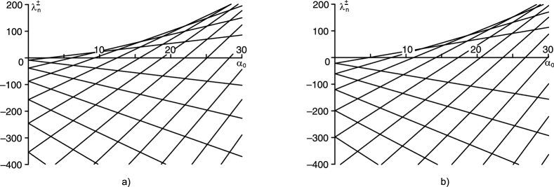
Figure 1: Eigenvalues $\lambda_{n}^{\pm}(\alpha_{0}\geq 0)$ for $l=0$ (a) and $l=1$ (b). The spectral branches intersect at semi-simple degeneration points (diabolical points) of algebraic and geometric multiplicity two.

In order to calculate the intersection points of the spectral branches (the nodes of the spectral mesh), we introduce the following convenient notation

$$\lambda_{n}^{\varepsilon} = -\rho_{n}+\varepsilon\alpha_{0}\sqrt{\rho_{n}}\,,\qquad\varepsilon=\pm$$

$$\mathfrak{u}_{n}^{\varepsilon} = \left(\begin{array}[]{c}1\\ \varepsilon\sqrt{\rho_{n}}\\ \end{array}\right)u_{n}\,,$$ (18)

which allows us to treat positive and negative Krein space states in a unified way.

Two branches $\lambda_{m}^{\delta},\lambda_{n}^{\varepsilon}$ with $n\neq m$ intersect at a point $(\alpha_{0}^{\nu},\lambda_{0}^{\nu})$ when

$$\begin{array}[]{rcl}\lambda_{n}^{\varepsilon}&=&\lambda_{m}^{\delta}\\ -\rho_{n}+\varepsilon\alpha_{0}\sqrt{\rho_{n}}&=&-\rho_{m}+\delta\alpha_{0}\sqrt{\rho_{m}}\\ \alpha_{0}&=&\frac{\rho_{n}-\rho_{m}}{\varepsilon\sqrt{\rho_{n}}-\delta\sqrt{\rho_{m}}}\\ \alpha_{0}^{\nu}:=\alpha_{0}&=&\varepsilon\sqrt{\rho_{n}}+\delta\sqrt{\rho_{m}}\end{array}$$

and hence

$$\lambda_{n}^{\varepsilon}=\lambda_{m}^{\delta}=\lambda_{0}^{\nu}:=\varepsilon\delta\sqrt{\rho_{n}\rho_{m}}\,.$$ (19)

Eqs. (2) and (19) imply that spectral branches of different type $\delta\neq\varepsilon$ intersect for both signs of $\alpha_{0}$ at $\lambda_{0}^{\nu}<0$. In contrast, intersections at $\lambda_{0}^{\nu}>0$ are induced by spectral branches of positive type when $\alpha_{0}>0$, and by spectral branches of negative type when $\alpha_{0}<0$.

According to equation (14) the double eigenvalue $\lambda_{0}^{\nu}$ possesses the two distinct eigenvectors $\mathfrak{u}_{n}^{\varepsilon}$ and $\mathfrak{u}_{m}^{\delta}$:

$$\mathfrak{u}_{n}^{\varepsilon}=\left(\begin{array}[]{c}1\\ \varepsilon\sqrt{\rho_{n}}\\ \end{array}\right)u_{n},\qquad\mathfrak{u}_{m}^{\delta}=\left(\begin{array}[]{c}1\\ \delta\sqrt{\rho_{m}}\\ \end{array}\right)u_{m}\,.$$ (20)

Consequently, the intersection points given by (2) correspond to double eigenvalues (19) with two linearly independent eigenvectors (20), i.e. they are semi-simple eigenvalues or diabolical points [12, 14, 15, 16] of algebraic and geometric multiplicity two.

3 Unfolding diabolical points by perturbations of the $\alpha$-profile

Let us assume that the operator $\mathfrak{A}_{\alpha_{0}^{\nu}}$ for $\alpha_{0}=\alpha_{0}^{\nu}$ has a semi-simple double eigenvalue $\lambda_{0}^{\nu}$ with eigenvectors $\mathfrak{u}_{n}^{\varepsilon}$ and $\mathfrak{u}_{m}^{\delta}$ determined by equations (19) and (20). Consider a perturbation of the $\alpha$-profile of the form

$$\alpha(r)=\alpha_{0}^{\nu}+\Delta\alpha(r)=\alpha_{0}^{\nu}+\epsilon\varphi(r)\,.$$ (21)

Then, the perturbed operator is given by

$$\mathfrak{A}_{\alpha}=\mathfrak{A}_{\alpha_{0}^{\nu}}+\epsilon\left(\begin{array}[]{cc}0&\varphi(r)\\ \varphi(r)A_{l}-\varphi^{\prime}(r)\partial_{r}&0\\ \end{array}\right)=:\mathfrak{A}_{\alpha_{0}^{\nu}}+\epsilon\mathfrak{B}$$ (22)

and the eigenvalue problem can be expanded in terms of the small parameter $\epsilon$ [14, 15, 16] as

$$(\mathfrak{A}_{\alpha_{0}^{\nu}}+\epsilon\mathfrak{B})(\mathfrak{u}_{0}^{\nu}+\epsilon\mathfrak{u}_{1}+\ldots)=(\lambda_{0}^{\nu}+\epsilon\lambda_{1}+\ldots)(\mathfrak{u}_{0}^{\nu}+\epsilon\mathfrak{u}_{1}+\ldots)\,.$$ (23)

Here, $\mathfrak{u}_{0}^{\nu}$ is an eigenvector of the unperturbed operator $\mathfrak{A}_{\alpha_{0}^{\nu}}$, corresponds to the eigenvalue $\lambda_{0}^{\nu}$ and, hence, has to be a linear combination of $\mathfrak{u}_{n}^{\varepsilon}$ and $\mathfrak{u}_{m}^{\delta}$

$$\mathfrak{u}_{0}^{\nu}=\gamma_{1}\mathfrak{u}_{n}^{\varepsilon}+\gamma_{2}\mathfrak{u}_{m}^{\delta}\in\mbox{\rm span}\!\left(\mathfrak{u}_{n}^{\varepsilon},\mathfrak{u}_{m}^{\delta}\right)\subset\mathcal{K}\,.$$ (24)

A comparison of the coefficients at the same powers of $\epsilon$ yields up to first order in $\epsilon$

$$\mathfrak{A}_{\alpha^{\nu}_{0}}\mathfrak{u}_{0}^{\nu}=\lambda_{0}^{\nu}\mathfrak{u}_{0}^{\nu}\,,$$ (25)

$$\mathfrak{A}_{\alpha^{\nu}_{0}}\mathfrak{u}_{1}+\mathfrak{B}\mathfrak{u}_{0}^{\nu}=\lambda_{0}^{\nu}\mathfrak{u}_{1}+\lambda_{1}\mathfrak{u}_{0}^{\nu}\,.$$ (26)

The first of these equations is satisfied identically, whereas the second one can be most conveniently analyzed by projecting it with the help of the Krein space inner product $[.,.]$ onto the two-dimensional subspace  $\mbox{\rm span}\!\left(\mathfrak{u}_{n}^{\varepsilon},\mathfrak{u}_{m}^{\delta}\right)\subset\mathcal{K}$

$$[\mathfrak{B}\mathfrak{u}_{0}^{\nu},\mathfrak{u}_{n}^{\varepsilon}]=\lambda_{1}[\mathfrak{u}_{0}^{\nu},\mathfrak{u}_{n}^{\varepsilon}],~{}~{}[\mathfrak{B}\mathfrak{u}_{0}^{\nu},\mathfrak{u}_{m}^{\delta}]=\lambda_{1}[\mathfrak{u}_{0}^{\nu},\mathfrak{u}_{m}^{\delta}]\,.$$ (27)

Using (24) in (27) yields a closed system of defining equations for the first order spectral perturbation $\lambda_{1}$ and the coefficients $\gamma_{1}$ and $\gamma_{2}$

$$\left(\begin{array}[]{cc}[\mathfrak{B}\mathfrak{u}_{n}^{\varepsilon},\mathfrak{u}_{n}^{\varepsilon}]-\lambda_{1}[\mathfrak{u}_{n}^{\varepsilon},\mathfrak{u}_{n}^{\varepsilon}]&[\mathfrak{B}\mathfrak{u}_{m}^{\delta},\mathfrak{u}_{n}^{\varepsilon}]\\ {}\hfil&{}\hfil\\ {[\mathfrak{B}\mathfrak{u}_{n}^{\varepsilon},\mathfrak{u}_{m}^{\delta}]}&[\mathfrak{B}\mathfrak{u}_{m}^{\delta},\mathfrak{u}_{m}^{\delta}]-\lambda_{1}[\mathfrak{u}_{m}^{\delta},\mathfrak{u}_{m}^{\delta}]\end{array}\right)\left(\begin{array}[]{c}\gamma_{1}\\ {}\hfil\\ \gamma_{2}\\ \end{array}\right)=0,$$ (28)

i.e. in first order approximation the perturbation $\epsilon\mathfrak{B}$ defines the spectral shift $\lambda_{1}$ and lifts the directional degeneration (24) of the zeroth order eigenvectors $\mathfrak{u}^{\nu}_{0}$ by fixing two rays in the subspace $\mbox{\rm span}\!\left(\mathfrak{u}_{n}^{\varepsilon},\mathfrak{u}_{m}^{\delta}\right)\subset\mathcal{K}$ (a standard effect known also from the perturbation theory of degenerate quantum mechanical systems [17]).

In our subsequent considerations of the system (28) we will need different explicit representations of the matrix elements containing $\mathfrak{B}$. Partial integration and substitution of the relation $\partial_{r}^{2}u_{n}=[-\rho_{n}+l(l+1)/r^{2}]u_{n}$ give these representations as

$$[\mathfrak{B}\mathfrak{u}_{m}^{\delta},\mathfrak{u}_{n}^{\varepsilon}] = \int_{0}^{1}\varphi\left[(\rho_{m}+\varepsilon\delta\sqrt{\rho_{n}\rho_{m}})u_{m}u_{n}+u_{m}^{\prime\prime}u_{n}+u_{m}^{\prime}u_{n}^{\prime}\right]dr$$ (29)

$$= \int_{0}^{1}\varphi\left[\left((\varepsilon\delta\sqrt{\rho_{n}\rho_{m}}+\frac{l(l+1)}{r^{2}}\right)u_{m}u_{n}+u_{m}^{\prime}u_{n}^{\prime}\right]dr\,.$$ (30)

The symmetry properties of Eq. (30) and its implication

$$[\mathfrak{B}\mathfrak{u}_{m}^{\delta},\mathfrak{u}_{n}^{\varepsilon}]=[\mathfrak{B}\mathfrak{u}_{n}^{\varepsilon},\mathfrak{u}_{m}^{\delta}]$$ (31)

are a natural consequence of the Krein space self-adjointness of the perturbation operator $\mathfrak{B}$ and the real-valuedness of the eigenvectors $\mathfrak{u}_{n}^{\varepsilon}$, $\mathfrak{u}_{m}^{\delta}$.

From (28) and (31) we obtain the following defining equation for $\lambda_{1}$

$$\lambda_{1}^{2}-\lambda_{1}\left(\frac{[\mathfrak{B}\mathfrak{u}_{n}^{\varepsilon},\mathfrak{u}_{n}^{\varepsilon}]}{[\mathfrak{u}_{n}^{\varepsilon},\mathfrak{u}_{n}^{\varepsilon}]}+\frac{[\mathfrak{B}\mathfrak{u}_{m}^{\delta},\mathfrak{u}_{m}^{\delta}]}{[\mathfrak{u}_{m}^{\delta},\mathfrak{u}_{m}^{\delta}]}\right)+\frac{[\mathfrak{B}\mathfrak{u}_{n}^{\varepsilon},\mathfrak{u}_{n}^{\varepsilon}][\mathfrak{B}\mathfrak{u}_{m}^{\delta},\mathfrak{u}_{m}^{\delta}]-[\mathfrak{B}\mathfrak{u}_{n}^{\varepsilon},\mathfrak{u}_{m}^{\delta}]^{2}}{[\mathfrak{u}_{n}^{\varepsilon},\mathfrak{u}_{n}^{\varepsilon}][\mathfrak{u}_{m}^{\delta},\mathfrak{u}_{m}^{\delta}]}=0$$ (32)

which with the Krein space norm (15) reduces to

$$\lambda_{1}^{2}-\lambda_{1}\left(\varepsilon\frac{[\mathfrak{B}\mathfrak{u}_{n}^{\varepsilon},\mathfrak{u}_{n}^{\varepsilon}]}{2\sqrt{\rho_{n}}}+\delta\frac{[\mathfrak{B}\mathfrak{u}_{m}^{\delta},\mathfrak{u}_{m}^{\delta}]}{2\sqrt{\rho_{m}}}\right)+\varepsilon\delta\frac{[\mathfrak{B}\mathfrak{u}_{n}^{\varepsilon},\mathfrak{u}_{n}^{\varepsilon}][\mathfrak{B}\mathfrak{u}_{m}^{\delta},\mathfrak{u}_{m}^{\delta}]-[\mathfrak{B}\mathfrak{u}_{n}^{\varepsilon},\mathfrak{u}_{m}^{\delta}]^{2}}{4\sqrt{\rho_{n}\rho_{m}}}=0\,.$$ (33)

This quadratic equation is of the type  $\lambda_{1}^{2}-\lambda_{1}(a_{1}+a_{2})+a_{1}a_{2}-\varepsilon\delta b^{2}/4=0,\ \ a_{1},a_{2},b\in\mathbb{R}$ and its solutions $\lambda_{1,\pm}=[(a_{1}+a_{2})\pm\sqrt{(a_{1}-a_{2})^{2}+\varepsilon\delta b^{2}}]/2$ are real-valued for $\varepsilon=\delta$ and complex for $\varepsilon\neq\delta\ \cap\ (a_{1}-a_{2})^{2}<b^{2}$ (in the present first order approximation). We see that they show the typical Krein space behavior. Intersections of spectral branches corresponding to Krein-space states of the same type $(\varepsilon=\delta)$ induce no real-to-complex transitions in the spectrum (they are weak interactions in the sense of [18]). In contrast, intersections of spectral branches corresponding to states of different types $(\varepsilon\neq\delta)$ may in general be accompanied by real-to-complex transitions (they are strong interactions in the sense of [18]). The same generic behavior is implicitly present, e.g., in the ${\cal PT}-$symmetric quantum mechanical (QM) models of Refs. [19, 20, 21, 22, 23] (see also the discussion in [24, 25]). The unfolding of a diabolical point in a Hermitian QM model under ${\cal PT}-$symmetric perturbations was explicitly demonstrated in Ref. [26].

As noted above, the unfolding of the diabolical points is accompanied with a fixing of the directions of the zeroth order eigenvectors $\mathfrak{u}^{\nu}_{0}\in\mbox{\rm span}\!\left(\mathfrak{u}_{n}^{\varepsilon},\mathfrak{u}_{m}^{\delta}\right)\subset\mathcal{K}$. Using $\lambda_{1,\pm}$ in (28) one finds these directions as rays $\mathfrak{u}^{\nu}_{0,\pm}=\gamma_{1,\pm}\mathfrak{u}_{n}^{\varepsilon}+\gamma_{2,\pm}\mathfrak{u}_{m}^{\delta}$ defined by

$$\frac{\gamma_{1,\pm}}{\gamma_{2,\pm}}=-\frac{[\mathfrak{B}\mathfrak{u}_{m}^{\delta},\mathfrak{u}_{n}^{\varepsilon}]}{[\mathfrak{B}\mathfrak{u}_{n}^{\varepsilon},\mathfrak{u}_{n}^{\varepsilon}]-[\mathfrak{u}_{n}^{\varepsilon},\mathfrak{u}_{n}^{\varepsilon}]\lambda_{1,\pm}}=-\frac{[\mathfrak{B}\mathfrak{u}_{m}^{\delta},\mathfrak{u}_{m}^{\delta}]-[\mathfrak{u}_{m}^{\delta},\mathfrak{u}_{m}^{\delta}]\lambda_{1,\pm}}{[\mathfrak{B}\mathfrak{u}_{n}^{\varepsilon},\mathfrak{u}_{m}^{\delta}]}$$ (34)

— a generic result obtained, e.g., also in [16].

As part of the subsequent considerations, we will apply the general technique (29), (30), (33) and (34) for a detailed analytical study of the unfolding of diabolical points in concrete dynamo setups.

4 Local deformations of the spectral mesh

The perturbation analysis of the previous section has been restricted to a first order approximation — giving trustworthy analytical results for the behavior of the spectrum in a very close vicinity of any single diabolical point. Here we extend this approximation method to parameter space regions ($\alpha_{0}-$regions) containing several diabolical points — allowing in this way to gain a qualitative understanding of how perturbations of the $\alpha-$profile deform the spectral mesh over such a region. For this purpose we extend the projection technique of the previous section from projecting on two-dimensional subspaces $\mbox{\rm span}\!\left(\mathfrak{u}_{n}^{\varepsilon},\mathfrak{u}_{m}^{\delta}\right)\subset\mathcal{K}$ to projections on $N-$dimensional subspaces $\mathcal{L}:=\mbox{\rm span}\!\left(\mathfrak{u}_{n_{1}}^{\varepsilon_{1}},\ldots,\mathfrak{u}_{n_{N}}^{\varepsilon_{N}}\right)\subset\mathcal{K}$ spanned by those eigenvectors which are involved in the intersections over the concrete region. The method is well known from computational mathematics as Galerkin method, Rayleigh-Ritz method or method of weighted residuals [27, 28, 29, 30, 31].

In order to simplify notations, we pass from double-indexed eigenvalues $\lambda_{n}^{\varepsilon}$ and states $\mathfrak{u}_{n}^{\varepsilon}\in\mathcal{K}_{\varepsilon}\subset\mathcal{K}_{+}\oplus\mathcal{K}_{-}\subset\mathcal{K}$ with $(n,\varepsilon)\in\mathbb{Z}^{+}\times\mathbb{Z}_{2}\sim\mathbb{Z}^{*}=\mathbb{Z}-\{0\}$ to eigenvalues $\lambda_{n}$ and normalized states $\mathfrak{v}_{n}$ depending only on the single state number $n\in\mathbb{Z}^{*}$:

$$\lambda_{n}=\left\{\begin{array}[]{ccc}\lambda_{n}^{+}&\mbox{for}&n\in\mathbb{Z}^{+}\\ \lambda_{|n|}^{-}&\mbox{for}&n\in\mathbb{Z}^{-}\\ \end{array}\right.,\qquad 2^{1/2}\rho_{n}^{1/4}\mathfrak{v}_{n}=\left\{\begin{array}[]{ccc}\mathfrak{u}_{n}^{+}\in\mathcal{K}_{+}&\mbox{for}&n\in\mathbb{Z}^{+}\\ \mathfrak{u}_{|n|}^{-}\in\mathcal{K}_{-}&\mbox{for}&n\in\mathbb{Z}^{-}\\ \end{array}\right.$$ (35)

with obvious implication

$$[\mathfrak{v}_{n},\mathfrak{v}_{m}]=\varepsilon_{n}\,\delta_{nm},\quad\varepsilon_{n}:=\mbox{\rm sign}\,(n)\,.$$ (36)

Furthermore, we order the index set of the vectors of the subspace $\mathcal{L}$ according to the rule $n_{1}>n_{2}>\ldots>n_{N}$ with $N_{+}$ vectors $\mathfrak{v}_{n}$ of positive type and $N_{-}=N-N_{+}$ of negative type.

The approximation of the eigenvalue problem (1) consists in representing the eigenfunction $\mathfrak{u}$ as linear combination

$$\mathfrak{u}=\sum_{i=k}^{N}c_{k}\mathfrak{v}_{n_{k}},\qquad c_{k}\in\mathbb{C}$$ (37)

over the finite set of basis functions $\{\mathfrak{v}_{n_{k}}\}_{k=1}^{N}$ and projecting the resulting equation

$$\sum_{i=1}^{N}c_{k}\left(\mathfrak{A}_{\alpha}-\lambda\right)\mathfrak{v}_{n_{k}}=0$$ (38)

onto the subspace $\mathcal{L}=\mbox{\rm span}\!\,(\mathfrak{v}_{n_{1}},\ldots,\mathfrak{v}_{n_{N}})\subset\mathcal{K}$. In terms of the notation

$$\tilde{\mathbf{A}}[\alpha]:=(\tilde{A}_{ij})_{i,j=1}^{N},\qquad\tilde{A}_{ij}:=\left[\mathfrak{A}_{\alpha}\mathfrak{v}_{n_{i}},\mathfrak{v}_{n_{j}}\right],$$

$$\boldsymbol{\eta}:=\mbox{\rm diag}\,(\varepsilon_{n_{1}},\ldots,\varepsilon_{n_{N}})=\left(\begin{array}[]{cc}I_{N_{+}}&0\\ 0&-I_{N_{-}}\end{array}\right),$$ (41)

$$\mathbf{c}:=(c_{1},\ldots,c_{N})^{T}\in\mathbb{C}^{N_{+}}\oplus\mathbb{C}^{N_{-}}$$ (42)

this leads to the simple $N\times N-$matrix eigenvalue problem

$$(\mathbf{A}[\alpha]-\lambda I_{N})\mathbf{c}=0,\qquad\mathbf{A}[\alpha]:=\boldsymbol{\eta}^{-1}\tilde{\mathbf{A}}[\alpha]$$ (43)

with

$$\det(\mathbf{A}[\alpha]-\lambda I_{N})=0$$ (44)

as defining equation for the spectral approximation. A few comments are in order here.

First, we note that the reality of the eigenvectors $\mathfrak{v}_{n}$ and of the dynamo operator $\mathfrak{A}_{\alpha}$ (cf. (2) and (14)) together with the selfadjointness of $\mathfrak{A}_{\alpha}$ in the Krein space $\mathcal{K}$ imply that the matrix $\tilde{\mathbf{A}}[\alpha]$ is real and symmetric, $\tilde{\mathbf{A}}^{T}[\alpha]=\tilde{\mathbf{A}}[\alpha]$. The Krein space related fundamental symmetry $\mathfrak{A}_{\alpha}=J\mathfrak{A}^{\dagger}_{\alpha}J$ (see (5)) is reflected in the structure of the matrix $\mathbf{A}[\alpha]=\boldsymbol{\eta}^{-1}\tilde{\mathbf{A}}[\alpha]$ as

$$\mathbf{A}[\alpha]=\boldsymbol{\eta}\mathbf{A}^{T}[\alpha]\boldsymbol{\eta}\,.$$ (45)

The involutory matrix $\boldsymbol{\eta}=\boldsymbol{\eta}^{-1}$ plays the role of a metric in the complex Pontryagin space $\pi_{\kappa}=\mathbb{C}^{N_{+}}\oplus\mathbb{C}^{N_{-}}\ni\mathbf{c}$. In fact, it holds for $\mathfrak{u}=\sum_{i=1}^{N}c_{i}\mathfrak{v}_{n_{i}},\ \mathfrak{w}=\sum_{j=1}^{N}d_{j}\mathfrak{v}_{n_{j}}$

$$[\mathfrak{u},\mathfrak{w}]=\sum_{i,j=1}^{N}\bar{c}_{i}d_{j}[\mathfrak{v}_{n_{i}},\mathfrak{v}_{n_{j}}]=\sum_{i=1}^{N}\varepsilon_{n_{i}}\bar{c}_{i}d_{i}=\bar{\mathbf{c}}^{T}\boldsymbol{\eta}\mathbf{d}\,.$$ (46)

Second, in the limit $N_{\pm}\to\infty$ the subspace $\mathcal{L}$ fills the whole Krein space $\mathcal{K}$ so that the approximation (37) of the vector $\mathfrak{u}$ tends to the exact representation $\mathfrak{u}=\sum_{n=-\infty}^{\infty}c_{n}\mathfrak{v}_{n}$ over the Krein space basis $\{\mathfrak{v}_{n}\}_{n=-\infty}^{\infty}$. In the same limit, the Pontryagin space $\pi_{\kappa}$ tends to the Krein space $\mathcal{S}=\mathcal{S}_{+}\oplus\mathcal{S}_{-}\ni\mathbf{c}$ with positive and negative type subspaces $\mathcal{S}_{\pm}$ as sequence spaces $\mathcal{S}_{\pm}=l_{2}(\mathbb{Z}^{\pm})$. The determinant (44) becomes a Hill type determinant. The mapping $U$ from the eigenvalue problem (1) in the function space $\mathcal{K}\ni\mathfrak{u}$ to its equivalent representation (43) in the sequence space $\mathcal{S}\ni\mathbf{c}$

$$U:\ \ (\mathfrak{A}_{\alpha}-\lambda)\mathfrak{u}=0\quad\mapsto\quad(\mathbf{A}[\alpha]-\lambda)\mathbf{c}=0$$ (47)

is the Krein space equivalent of the well known mapping from the quantum mechanical Schrödinger picture to its infinite-matrix representation in the Heisenberg picture [17]. In this sense, the described Galerkin method can be understood as an approximate solution technique based on a ’truncated Heisenberg representation’ of the eigenvalue problem. Obviously, the method is not restricted to $\alpha^{2}-$dynamo setups, rather in its present form it is applicable to any other Krein-space related setup as well, like e.g. models of $\mathcal{P}\mathcal{T}-$symmetric quantum mechanics. The only ingredient needed is a set of exactly known basis functions of an unperturbed operator.

In the next section, we use the described Galerkin method for a rough numerical analysis of the deformations of the spectral mesh in the region depicted in Fig. 1 — leaving analytical estimates of the residual (the approximation error) to forthcoming work.

5 The hyper-idealized $s-$wave $(l=0)$ sector and its $\bi{\alpha}-$resonance patterns

In this section, we consider the hyper-idealized case of zero spherical harmonics, $l=0$, which in analogy to quantum scattering theory can be interpreted as $s-$wave sector. Due to its too high symmetry contents, this sector does not play a role in the physics of spherical dynamos. There are no $s-$wave dynamos at all [2, 4]. Instead, it can be understood as a disk dynamo model [32] — in the concrete case of boundary conditions (4), as a disk dynamo with formal boundary conditions corresponding to a high-conductivity limit. Due to the strong spectral similarities of models with $l=1$ and $l=0$ (visible e.g. in Fig. 1), the study of disk dynamo models turns out very instructive from a technical point of view. Due to their highly simplified structure they allow for a detailed analytical handling and a transparent demonstration of some of the essential mathematical features of the dynamo models. In our concrete context, they will provide some basic intuitive insight into the dynamo related specifics of the unfolding of diabolical points. In the $(l\geq 1)-$sectors of the spherical models, these specifics will re-appear in a similar but more complicated way (see section 6 below).

Subsequently, we perform an analytical study of the local unfolding of the diabolical points (along the lines of Section 3) that we supplement by numerical Galerkin results on the deformation of the spectral mesh.

Let $l=0$. Then the differential expression of the operator $A_{l=0}$ reads simply $A_{l=0}=-\partial_{r}^{2}$ and $A_{l=0}$ has ortho-normalized eigenfunctions $u_{n}(r)$, $u_{n}(0)=u_{n}(1)=0$ and eigenvalues $\rho_{n}$

$$u_{n}=\sqrt{2}\sin(n\pi r),\qquad\rho_{n}=(\pi n)^{2}\,.$$ (48)

The eigenvalues of the matrix differential operator $\mathfrak{A}_{\alpha_{0}}$ are given as

$$\lambda_{n}^{\varepsilon}=-(\pi n)^{2}+\varepsilon\alpha_{0}\pi n$$ (49)

and the corresponding eigenvectors $\mathfrak{u}_{n}^{\varepsilon}$ yield Krein space inner products

$$\left[\mathfrak{u}_{n}^{\varepsilon},\mathfrak{u}_{m}^{\delta}\right]=\varepsilon 2\pi n\delta_{\varepsilon\delta}\delta_{mn}$$ (50)

and perturbation terms

$$[\mathfrak{B}\mathfrak{u}_{m}^{\delta},\mathfrak{u}_{n}^{\varepsilon}]=2\pi^{2}mn\int_{0}^{1}\varphi(r)\cos\left[(\delta m-\varepsilon n)\pi r\right]dr\,.$$ (51)

According to (2), the diabolical points are located at points

$$\alpha_{0}^{\nu}=\pi(\varepsilon n+\delta m)=:\pi M,\qquad\lambda_{0}^{\nu}=\varepsilon\delta\pi^{2}mn$$ (52)

and form a periodic vertical line structure in the $(\alpha_{0},\Re\lambda)-$plane.

Inspection of the defining equation (32) for the first order spectral perturbations $\lambda_{1}$ shows that this equation is invariant with regard to a re-scaling of $\mathfrak{u}_{n}^{\varepsilon},\mathfrak{u}_{m}^{\delta}$. Passing to the single-index notation (35) yields

$$\lambda_{n}=-(\pi n)^{2}+\alpha_{0}\pi n,~{}~{}\mathfrak{v}_{n}(r)=\frac{1}{\sqrt{\pi|n|}}\left(\begin{array}[]{c}1\\ \pi n\\ \end{array}\right)\sin(\pi|n|r),\quad n\in\mathbb{Z}^{*}$$ (53)

with $[\mathfrak{v}_{n},\mathfrak{v}_{m}]=\varepsilon_{n}\delta_{nm}$ and the following convenient representation of the perturbation terms (51)

$$[\mathfrak{B}\mathfrak{v}_{n+j},\mathfrak{v}_{n}]=\pi\sqrt{|n(n+j)|}\int_{0}^{1}\varphi(r)\cos(j\pi r)dr\,.$$ (54)

This reduces the defining equation (33) for the spectral perturbation at the $(n,n+j)$ node of the spectral mesh (the intersection point of the $\lambda_{n}$ and $\lambda_{n+j}$ branches of the spectrum) with coordinates

$$\alpha_{0}^{\nu}=\pi(2n+j)=:\pi M,\qquad\lambda_{0}^{\nu}=\pi^{2}n(n+j)$$ (55)

to

$$\lambda_{1}^{2}-\lambda_{1}\pi(2n+j)\int_{0}^{1}\varphi(r)dr+$$

$$+\pi^{2}n(n+j)\left[\left(\int_{0}^{1}\varphi(r)dr\right)^{2}-\left(\int_{0}^{1}\varphi(r)\cos(j\pi r)dr\right)^{2}\right]=0$$ (56)

with solutions

$$\lambda_{1,\pm}= \frac{\pi}{2}(2n+j)\int_{0}^{1}\varphi(r)dr$$ (57)

$$\pm\frac{\pi}{2}\sqrt{j^{2}\left(\int_{0}^{1}\varphi(r)dr\right)^{2}+4n(n+j)\left(\int_{0}^{1}\varphi(r)\cos(j\pi r)dr\right)^{2}}.$$

We observe that the strength of the complex valued unfolding of a diabolical point at a node with $n(n+j)<0$ is defined by the relation between its $\cos(j\pi r)-$filtered perturbation $\int_{0}^{1}\varphi(r)\cos(j\pi r)dr$ and its average perturbation $\int_{0}^{1}\varphi(r)dr$.

A deeper insight into this peculiar feature of the unfolding process can be gained by expanding the perturbation $\varphi$ in Fourier components over the interval $[0,1]$

$$\varphi(r)=\frac{a_{0}}{2}+\sum_{k=1}^{\infty}\left[a_{k}\cos(2\pi kr)+b_{k}\sin(2\pi kr)\right]$$ (58)

with coefficients given as $a_{0}=2\int_{0}^{1}\varphi(r)dr$,   $a_{k}=2\int_{0}^{1}\varphi(r)\cos(2\pi kr)dr$,   $b_{k}=2\int_{0}^{1}\varphi(r)\sin(2\pi kr)dr.$ In this way the integral $\int_{0}^{1}\varphi(r)\cos(j\pi r)dr$ in (54) reduces to components of the type

$$\int_{0}^{1}\cos(j\pi r)dr = \delta_{j,0}\,,$$

$$\int_{0}^{1}\cos(2\pi kr)\cos(j\pi r)dr = \frac{1}{2}\left(\delta_{j,2k}+\delta_{-j,2k}\right)\,,$$

$$\int_{0}^{1}\sin(2\pi kr)\cos(j\pi r)dr = \left\{\begin{array}[]{lcc}0&\mbox{\rm for}&j=\pm 2k\\ \\ \frac{1-(-1)^{j}}{\pi}\frac{2k}{4k^{2}-j^{2}}&\mbox{\rm for}&j\neq\pm 2k\end{array}\right.$$ (62)

and we obtain the perturbation terms (54) as

$$[\mathfrak{B}\mathfrak{v}_{n+j},\mathfrak{v}_{n}]=\frac{\pi}{2}\sqrt{|n(n+j)|}Q_{j}\,,$$ (63)

$$Q_{j}:=a_{0}\delta_{j,0}+\sum_{k=1}^{\infty}\left[a_{k}\left(\delta_{j,2k}+\delta_{-j,2k}\right)+\frac{1-(-1)^{j}}{\pi}\frac{4b_{k}k}{4k^{2}-j^{2}}\right].$$ (64)

The defining quadratic equation for the spectral perturbation $\lambda_{1}$ takes now the form

$$\lambda_{1}^{2}-\lambda_{1}\frac{\pi}{2}(2n+j)a_{0}+\frac{\pi^{2}}{4}n(n+j)\left(a_{0}^{2}-Q_{j}^{2}\right)=0$$ (65)

and leads to the following very instructive representation for its solutions

$$\lambda_{1,\pm}=\frac{\pi}{4}\left[(2n+j)a_{0}\pm\sqrt{j^{2}a_{0}^{2}+4n(n+j)Q_{j}^{2}}\right].$$ (66)

The structure of these solutions shows that the unfolding of the diabolical points is controlled by several, partially competing, effects. Apart from the above mentioned Krein space related feature of unfolding into real eigenvalues for states of the same Krein space type $(n(n+j)>0)$, and the possibility for unfolding into pairwise complex conjugate eigenvalues in case of states of opposite type $(n(n+j)<0)$ a competition occurs between oscillating perturbations $(a_{k\neq 0},b_{k})$ and homogeneous offset-shifts $a_{0}$. In the case of vanishing offset-shifts (mean perturbations), $a_{0}=0$, any inhomogeneous perturbation with $a_{k},b_{k}\neq 0$ for some $k\geq 1$ leads for two branches with $n(n+j)<0$ to a complex unfolding of the diabolical point. The strength of this complex directed unfolding becomes weaker when the homogeneous offset perturbation is switched on ($a_{0}\neq 0$). There exists a critical offset

$$a_{0(c)}^{2}:=-\frac{4n(n+j)}{j^{2}}Q^{2}_{j}$$ (67)

which separates the regions of real-valued and complex-valued unfoldings (in the present first-order approximation). For $a_{0}^{2}<a_{0(c)}^{2}\ \cap\ n(n+j)<0$ a complex-valued unfolding occurs, whereas for $a_{0}^{2}>a_{0(c)}^{2}\ \cap\ n(n+j)<0$ the diabolical point unfolds real-valued. The special case of a critical (balanced) perturbation $a_{0}^{2}=a_{0(c)}^{2}\ \cap\ n(n+j)<0$ corresponds to an eigenvalue degeneration $\lambda_{1,+}=\lambda_{1,-}=:\lambda_{1(c)}$ which, because of (34), (35) and $\gamma_{1,+}\gamma_{2,+}^{-1}=\gamma_{1,-}\gamma_{2,-}^{-1}\,$, has coinciding zeroth order rays so that via appropriate normalization the corresponding vectors $\mathfrak{v}^{\nu}_{0,+},\mathfrak{v}^{\nu}_{0,-}$ can be made coinciding $\mathfrak{v}^{\nu}_{0,+}=\mathfrak{v}^{\nu}_{0,-}=:\mathfrak{v}^{\nu}_{0(c)}$. This means that the original diabolical point splits into a pair of exceptional (branch) points at perturbation configurations $a_{0}=\pm|a_{0(c)}|$ with a Jordan chain consisting of the single (geometric) eigenvector (ray) $\mathfrak{v}^{\nu}_{0(c)}$ supplemented by an associated vector (algebraic eigenvector). This is in agreement with the unfolding scenario of diabolical points of general-type complex matrices described e.g. in [16].

Finally, the special case of $j=-2n$ is of interest. It corresponds to the intersection points located on the $(\alpha_{0}=0)-$axis of the $(\alpha_{0},\Re\lambda)-$plane, where the operator matrix is not only self-adjoint in the Krein space $\mathcal{K}$, but also in the Hilbert space $\tilde{\mathcal{H}}$. Due to the vanishing factor $2n+j$ these diabolical points unfold via perturbations $\lambda_{1}=\pm(\pi/2)|n|\sqrt{a_{0}^{2}-a_{|n|}^{2}}$.

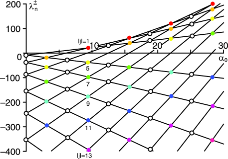
Figure 2: Odd harmonics of $\alpha(r)$ define the unfolding properties only of the colored diabolical points (equally colored DPs correspond to the same value of $|j|$), whereas even harmonics affect only the white (uncolored) DPs.

Let us now consider the strength of the unfolding contributions induced by certain Fourier components. For this purpose, we note that the diabolical points at nodes $(n,n+j)$ with the same absolute value of the index $j$ are located on a parabolic curve

$$\lambda_{0}^{\nu}=\frac{1}{4}({\alpha_{0}^{\nu}}^{2}-\pi^{2}j^{2})=\frac{\pi^{2}}{4}(M^{2}-j^{2})\,.$$ (68)

Due to its special role, we will refer to $j\in\mathbb{Z}$ as parabola index ($M\in\mathbb{Z}$ is the index of the vertical line in the $(\alpha_{0},\Re\lambda)-$plane defined in (52) and (55)). Furthermore, we see from the explicit structure of $Q_{j}$ (following from expression (64))

$$Q_{j}=\left\{\begin{array}[]{ll}\frac{8}{\pi}\sum_{k=1}^{\infty}b_{k}\frac{k}{4k^{2}-j^{2}}\,,&j=\pm 1,\pm 3,\ldots\\ a_{k}\left(\delta_{j,2k}+\delta_{-j,2k}\right)\,,&j=\pm 2,\pm 4,\ldots\end{array}\right.$$ (69)

that cosine and sine components of a similar order $|a_{k}|\sim|b_{k}|$ contribute differently at different nodes of the spectral mesh. It is remarkable that for all DPs with the same even $|j/2|$ (parabolas consisting of white points in Fig. 2), the splitting of the corresponding double eigenvalues depends (modulo the pre-factors $4n(n+j)$, $j^{2}$) only on the mean value $a_{0}$ of the perturbation $\varphi(r)$ and its $|j/2|$-th cosine component $a_{|j/2|}$. For $n(n+j)<0$ these contributions are competing, whereas for a strictly real-valued unfolding $n(n+j)>0$ they enhance each other. Furthermore, we find from $M:=2n+j$ that the even/odd mode properties of $j$ imply the same properties for $M$: even (odd) modes affect the unfolding of diabolical points at even (odd) $M$ only. This is also clearly visible from Fig. 2.

In the more complicated case of odd parabola indices $|j|$ the splitting of the diabolical points on the parabola (68) (in Fig. 2 they are marked as points of the same color) is governed by the competition between $a_{0}$ and the complete set of sine components $b_{k}$ of the perturbation $\varphi(r)$. According to (69), a dominant role is played by sine harmonics with $j^{2}\approx 4k^{2}$, i.e. with $k_{\pm}=(|j|\pm 1)/2$, such that a clear resonance and damping pattern occurs. Sine components with $j^{2}\approx 4k^{2}$ are highly enhanced by a small denominator over the other sine components and the corresponding harmonics can be regarded as resonant ones. In contrast, sine contributions with modes away from the resonant $k_{\pm}=(|j|\pm 1)/2$ are strongly damped by the denominator $4k^{2}-j^{2}$ and tend asymptotically to zero for $j^{2}\to\infty$.

A first order approximation based insight into this asymptotical behavior can be gained from the positions of the exceptional points (EPs) in the $(\alpha_{0},\Re\lambda)-$plane (the points where real-to-complex transitions occur). For this purpose, we use a 1D-lattice type parametrization for $\alpha_{0}$ in form of $\alpha_{0}=\alpha_{0}^{\nu}+\Delta\alpha_{0}=\pi M+\Delta\alpha_{0},\ M\in\mathbb{Z}$ and switch to a setting with $\epsilon=1$ and $\Delta\alpha(r):=\phi(r)$. Interpreting $\Delta\alpha_{0}$ as perturbation of a configuration with $\alpha_{0}^{\nu}=\pi M$ allows us to relate $\Delta\alpha_{0}$ to the Fourier coefficient $a_{0}=2\Delta\alpha_{0}$ and to estimate the $\alpha_{0}-$positions of the EPs $\Delta\alpha_{e}(M,j)$ relative to their corresponding diabolical points located on the line $\alpha_{0}^{\nu}=\pi M$. Via (67) and $n=(M-j)/2$ we get for given $Q_{j}$

$$\left[\Delta\alpha_{e}(M,j)\right]^{2}=-\frac{n(n+j)}{j^{2}}Q_{j}^{2}=\frac{1}{4}\left(1-\frac{M^{2}}{j^{2}}\right)Q^{2}_{j}\,.$$ (70)

For diabolical points in the lower $(\alpha_{0},\Re\lambda)-$half-plane it holds $|j|\geq|M|+2$ and (70) is well defined. In the case of cosine perturbations $a_{k}\cos(2\pi kr)$, (69) implies that only a single diabolical point per $M=0,\pm 2,\pm 4,\ldots$ unfolds, whereas for sine perturbations $b_{k}\sin(2\pi kr)$ it leads to a countably infinite number of unfolding diabolical points per $M=\pm 1,\pm 2,\ldots$. Substituting (69) into (70) one obtains the $M^{2},k^{2}\ll j^{2}\to\infty$ asymptotics of the EP positions as

$$|\Delta\alpha_{e}(M,j)|\approx\frac{4|b_{k}|k}{\pi j^{2}},$$ (71)

i.e. for increasing $j^{2}$ the distance of the EPs from the DPs is tending to zero. Conversely, (71) may be used to give an estimate for the number of complex eigenvalues for a given $\alpha_{0}=\pi M+\Delta\alpha_{0}$ close to a diabolical point line at $\alpha_{0}\approx\pi M$, $|\Delta\alpha_{0}|\ll\pi$:  $j^{2}\approx 4|b_{k}|k/(\pi|\Delta\alpha_{0}|).$

Above, we arrived at the conclusion that both types of $|j|-$nodes (even ones and odd ones) show a similar collective behavior along the parabolic curves (68) of fixed $j^{2}$, responding on some specific $\alpha-$perturbation harmonics in a resonant way. Hence, a specific $\alpha-$resonance pattern is imprinted in the spectral unfolding picture of the diabolical points.

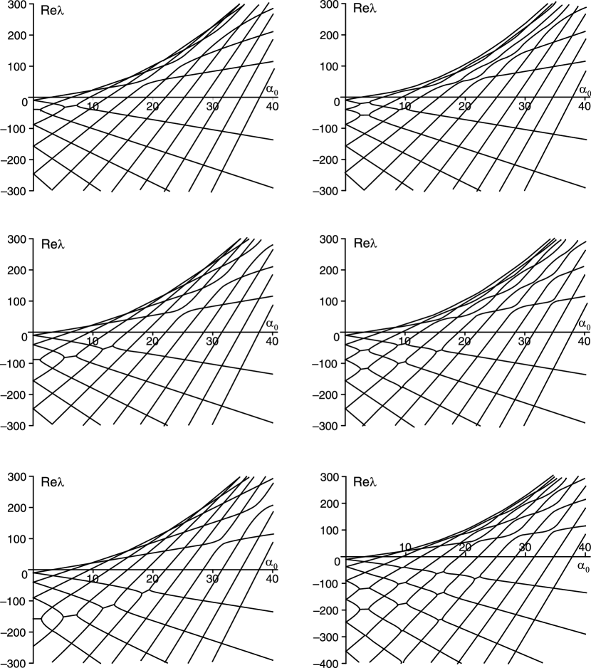
Figure 3: Resonant deformation of the spectral mesh with resonant unfolding of diabolical points due to perturbations by pure harmonics. Left column top down $\Delta\alpha(r)=2.5\cos(4\pi r)$, $\Delta\alpha(r)=2.5\cos(6\pi r)$, $\Delta\alpha(r)=2.5\cos(8\pi r)$; right column top down $\Delta\alpha(r)=2.5\sin(4\pi r)$, $\Delta\alpha(r)=2.5\sin(6\pi r)$, $\Delta\alpha(r)=2.5\sin(8\pi r)$.

Let us now analyze these $\alpha-$resonance patterns as imprints in the deformations of the spectral mesh. We study these deformations with the help of a Galerkin approximation over a 24-dimensional Krein subspace $\mathcal{L}=\mbox{\rm span}\!(\mathfrak{v}_{12},\ldots,\mathfrak{v}_{-12})\subset\mathcal{K}$ — which is sufficient to cover the same spectral region as in Fig. 1. As $\alpha-$profile we choose $\alpha(r)=\alpha_{0}+\Delta\alpha(r)$ with pure harmonics $\Delta\alpha(r)=a_{k}\cos(2\pi kr)$ and $\Delta\alpha(r)=b_{k}\sin(2\pi kr)$, $k=2,3,4$,  $a_{k}=b_{k}=5/2$ as perturbations. The explicit structure of the corresponding Pontryagin space related matrix $\mathbf{A}[\alpha]$ (see (43)) is given in B and yields the spectral approximations depicted in Fig. 3.

The most striking feature of the spectral deformations is their very clearly pronounced resonance character along parabolas with fixed index $|j|$ — leaving spectral regions away from these resonance parabolas almost unaffected. Specifically, we find for cosine perturbations (depicted in the left column) that the harmonics $k=2,3,4$ affect only the unfolding of diabolical points located strictly on the associated parabolas with index $j=2k$. The effect of sine perturbations with mode numbers $k=2,3,4$ is shown in the right column graphics of Fig. 3. As predicted by (69), we find a strongly pronounced unfolding of diabolical points located on the parabolas with $|j|=2k\pm 1$, that is for $|j|=3$ and $|j|=5$ (upper right picture), $|j|=5$ and $|j|=7$ (middle right), and $|j|=7$ and $|j|=9$ (lower right picture). The DPs with $|j|=2k\pm m$, $m>1$ are less affected and the strength of the unfolding quickly decreases with increasing distance $m$ to the resonant parabolas. In addition to the unfolding effects predicted analytically by first order perturbation theory, the top and middle right pictures show additional DP unfoldings on the large$-\alpha_{0}-$end of the $|j|=2k$ parabola. The origin of these unfoldings can be attributed to higher-order perturbative contributions.

The $\alpha-$resonance pattern has a simple physical interpretation. Due to the fact that the spectral parameter implies an $e^{\lambda t}$ behavior of the corresponding field mode, the $\alpha-$resonance pattern shows that short scale perturbations of the $\alpha-$profile (Fourier components with higher $k$) coherently affect faster decaying (more negative $\Re\lambda$) field modes than large scale perturbations with smaller $k$ (which lead to smaller negative $\Re\lambda$).

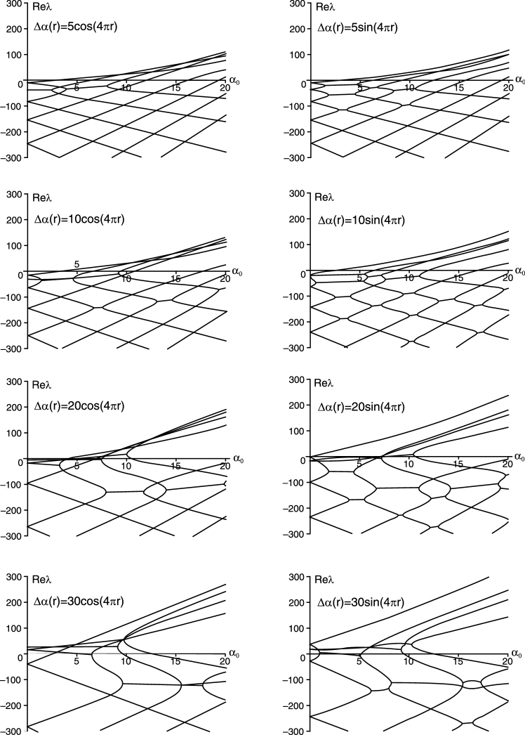
Figure 4: Resonant deformation of the spectral mesh under strong and ultra-strong perturbations of pure harmonic type: $\Delta\alpha(r)=a_{2}\cos(4\pi r)$ (left column) and $\Delta\alpha(r)=b_{2}\sin(4\pi r)$ (right column) with $a_{2},b_{2}=5,10,20,30$. Strong perturbations lead not only to large spectral regions with complex conjugate eigenvalues, but also to a lifting of the corresponding complex branches into the upper $(\alpha_{0},\Re\lambda)-$plane, i.e. they lead to overcritical dynamo regimes ($\Re\lambda>0$) of oscillatory type ($\Im\lambda\neq 0$).

Up to now we used the Galerkin method for investigations of weak perturbations over an $\alpha_{0}=$const background. In Fig. 4 we demonstrate that the method works for strong perturbations as well. We observe that, increasing the strength of the pure harmonic perturbations from $a_{2},b_{2}=5$ up to $a_{2},b_{2}=30$, the regions with complex conjugate spectral contributions grow and finally intersect each other. Additionally, they shift into the upper $(\alpha_{0},\Re\lambda)-$plane leading to overcritical oscillatory dynamo regimes $(\Re\lambda>0,\Im\lambda\neq 0)$. An estimate of critical $\alpha-$profiles, for which such a transition to the upper $(\alpha_{0},\Re\lambda)-$half-plane starts to occur, can be given within a first-order (linear) perturbative approximation by assuming $\Re\lambda(\alpha_{0})=0$ for the exceptional point closest to the $(\Re\lambda=0)-$line. Relations (68), (70) and $\Re\lambda=\lambda_{0}^{\nu}+\Re\lambda_{1}=\lambda_{0}^{\nu}+\pi Ma_{0}/4$ yield this condition in terms of the Fourier components $Q_{j}$ of such a critical $\alpha-$profile as

$$\Re\lambda=\frac{\pi^{2}}{4}\left(M^{2}-j^{2}\right)+\frac{\pi}{4}M\left(1-\frac{M^{2}}{j^{2}}\right)^{1/2}|Q_{j}|=0.$$ (72)

This relation may be used for testing concrete $\alpha-$profiles on their capability to produce complex eigenvalues in the right spectral half-plane $(\Re\lambda>0,\Im\lambda\neq 0)$.

We restrict our present consideration of $(l=0)-$models to this first numerical output and the analytical estimate, expecting physically more relevant results from extending the present methods to models with physically realistic boundary conditions. In the next section we present some first few results on the $(l\geq 1)-$sectors of the $\alpha^{2}-$dynamo model.

6 Numerical techniques and examples for the $(l\geq 1)-$sectors

In this section, we reshape the general results of section 3 in a form suitable for numerical investigations and demonstrate them on a first concrete model from the $(l=1)-$sector.

We start by representing the perturbation terms $[\mathfrak{B}\mathfrak{u}_{m}^{\delta},\mathfrak{u}_{n}^{\varepsilon}]$ from Eqs. (29), (30) as

$$[\mathfrak{B}\mathfrak{u}_{m}^{\delta},\mathfrak{u}_{n}^{\varepsilon}] = \int_{0}^{1}\varphi\left[\left(\varepsilon\delta\sqrt{\rho_{m}\rho_{n}}+\frac{l(l+1)}{r^{2}}\right)u_{m}u_{n}+u_{m}^{\prime}u_{n}^{\prime}\right]dr$$ (73)

$$= 2(\rho_{m}\rho_{n})^{1/4}\int_{0}^{1}\varphi(r)g_{mn}^{l}(r)dr,\quad m,n\in\mathbb{Z}^{+}$$

or equivalently

$$[\mathfrak{B}\mathfrak{v}_{m},\mathfrak{v}_{n}] = \int_{0}^{1}\varphi\left[\left(\varepsilon_{m}\varepsilon_{n}\sqrt{\rho_{|m|}\rho_{|n|}}+\frac{l(l+1)}{r^{2}}\right)u_{|m|}u_{|n|}+u_{|m|}^{\prime}u_{|n|}^{\prime}\right]dr$$ (74)

$$= \int_{0}^{1}\varphi(r)g_{mn}^{l}(r)dr,\quad m,n\in\mathbb{Z}^{*}\,.$$

The functions $g_{mn}^{l}$ are symmetric $g_{mn}^{l}=g_{nm}^{l}$ and from the Fréchet (functional) derivative

$$\frac{\delta[\mathfrak{B}\mathfrak{v}_{m},\mathfrak{v}_{n}]}{\delta\varphi(r)}\equiv\nabla_{\varphi}[\mathfrak{B}\mathfrak{v}_{m},\mathfrak{v}_{n}]=g_{mn}^{l}(r)$$ (75)

we find that they can be naturally interpreted as components of the perturbation gradient in the Krein space $\mathcal{K}$. Their explicit representation in terms of Bessel functions is given in C. Representation (73) may prove especially useful for the optimization of $\alpha$-profiles with regard to given constraints or experimental requirements.

First, we note that in terms of the gradient functions $g_{mn}^{l}(r)$ the defining equation (33) for the first order spectral perturbations $\lambda_{1}$ reduces to

$$\lambda_{1}^{2}-\lambda_{1}\int_{0}^{1}\varphi\left(\varepsilon g^{l}_{nn}+\delta g^{l}_{mm}\right)dr+$$

$$+\varepsilon\delta\left[\left(\int_{0}^{1}\varphi g^{l}_{mm}dr\right)\left(\int_{0}^{1}\varphi g^{l}_{nn}dr\right)-\left(\int_{0}^{1}\varphi g^{l}_{mn}dr\right)^{2}\right]=0$$ (76)

with solutions

$$\lambda_{1,\pm}=\frac{1}{2}\int_{0}^{1}\varphi\left(\varepsilon g^{l}_{nn}+\delta g^{l}_{mm}\right)dr$$

$$\pm\frac{1}{2}\sqrt{\left[\int_{0}^{1}\varphi\left(\varepsilon g^{l}_{nn}-\delta g^{l}_{mm}\right)dr\right]^{2}+4\varepsilon\delta\left[\int_{0}^{1}\varphi g^{l}_{mn}dr\right]^{2}}.$$ (77)

Comparison with the results for the hyper-idealized $s-$wave sector (disk dynamo) shows that apart from the generic Krein space related behavior (no complex eigenvalues for intersecting spectral branches of the same type, $\delta=\varepsilon$, and possible formation of complex eigenvalues for branches of different type, $\varepsilon\neq\delta$) we find a generalization of the offset and oscillation contributions for $\varepsilon\neq\delta$ type intersections. In rough analogy, the role of a transition preventing offset is played by the ’diagonal’ terms

$$\int_{0}^{1}\varphi\left(g^{l}_{nn}+g^{l}_{mm}\right)dr$$ (78)

whereas the ’off-diagonal’ terms

$$\left[\int_{0}^{1}\varphi g^{l}_{mn}dr\right]^{2}$$ (79)

enhance a possible transitions to complex eigenvalues, i.e. a transition occurs for

$$\varepsilon\neq\delta\quad\cap\quad\left(\frac{1}{2}\int_{0}^{1}\left(g^{l}_{nn}+g^{l}_{mm}\right)\varphi dr\right)^{2}<\left(\int_{0}^{1}g_{mn}^{l}\varphi dr\right)^{2}.$$ (80)

The condition (80) yields an explicit classification criterion for $\alpha-$profile perturbations with regard to their capability to induce complex eigenvalues. It may serve as an efficient search tool for concrete $\alpha(r)-$profiles — and transforms in this way some general observations of Ref. [4] into a technique of direct applicability.

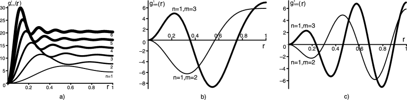
Figure 5: Functions $g_{nm}^{l}(r)$ for $l=1$, $n=m$ (a) and $n=1$, $m=2,3$ in the cases $\varepsilon\delta=1$ (b) and $\varepsilon\delta=-1$ (c).

The functions $g_{nm}^{l}(r)$ for $l=1$ and different values of $n$, $m$ and $\epsilon\delta$ are shown in Fig (2). One clearly sees that the ’diagonal’ functions with $m=n$ are always non-negative and the graphics of any two of them, $g_{nn}^{1}(r)$, $g_{mm}^{1}(r)$ with $m\neq n$ intersect only marginally (see Fig. 6). Their sums $g_{nn}^{1}(r)+g_{mm}^{1}(r)$ are strictly sign-preserving functions so that they act as averaging integration kernels. In contrast, the ’off-diagonal’ functions $g_{nm}^{1}(r)$ with $m\neq n$ show strong sign changes and in this way they act as filter kernels. Hence, the main qualitative roles of the ’diagonal’ and ’off-diagonal’ functions as ’offset’ and ’oscillation filter’ functions remain preserved also for the $(l=1)-$sector.

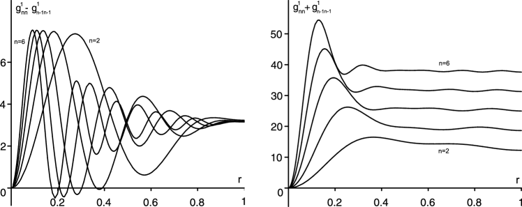
Figure 6: Gradient function differences $g_{nn}^{1}(r)-g_{n-1\,n-1}^{1}(r)$ as they enhance the real valued unfolding of diabolical points in the upper $(\alpha_{0},\Re\lambda)-$plane (left figure), as well as offset gradient functions (integration kernels) of the type $g_{nn}^{1}(r)+g_{n-1\,n-1}^{1}(r)$ for $n=2,\ldots,6$ (right figure).

Their subtle interplay is crucial for the $\alpha$-profile to act as generator of complex eigenvalues.

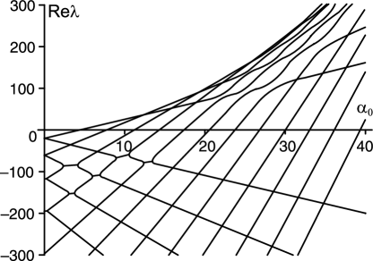
Figure 7: Deformations of the spectral mesh with unfolding of diabolical points for the $(l=1)-$sector of a model with $\alpha(r)=\alpha_{0}+2.5\cos(6\pi r)$.

As in the $(l=0)-$sector, spectral deformations over a certain parameter space region can be studied numerically. For $\alpha-$profiles $\alpha(r)=\alpha_{0}+\Delta\alpha(r)$ the corresponding approximation matrix of the Galerkin method reads simply

$$A_{mn}[\alpha]=\lambda_{m}\delta_{mn}+\varepsilon_{m}\int_{0}^{1}\Delta\alpha(r)g_{mn}^{l}(r)dr\,.$$ (81)

In Fig. 7 we illustrate the method for an $\alpha-$profile $\alpha(r)=\alpha_{0}+2.5\cos(6\pi r)$ and a similar approximation subspace $\mathcal{L}=\mbox{\rm span}\!(\mathfrak{v}_{12},\ldots,\mathfrak{v}_{-12})\subset\mathcal{K}$ as in the previous section. For the $(l=1)-$mode Riccati-Bessel functions a cosine perturbation is no longer an exact resonance mode and the deformations of the mesh are spreading over a broader parabola-like region.

Finally, we note that explicit analytical considerations of the spectrum in the $(l>0)-$sector are obstructed by the lack of simple transformation rules between Riccati-Bessel functions as well as of simple expressions for integrals over triple products of spherical Bessel functions in case of finite integration intervals.

7 Conclusions and discussions

In the present work, the spectral properties of spherically symmetric MHD $\alpha^{2}-$dynamos with idealized boundary conditions have been studied. Using the fundamental symmetry of the dynamo operator matrix and the solution set of a model with constant $\alpha-$profile, a Krein space related perturbation theory as well as a Galerkin technique for numerical investigations have been developed. As analytical result of the first-order perturbation theory we found a strongly pronounced $\alpha-$resonance pattern in the unfolding of diabolical points. The resonance behavior reflects the correspondence between the characteristic length scale of $\alpha-$perturbations and the decay rates of the coherently induced field excitations. The observed correlations will strongly affect the specifics of reversal processes of dynamo maintained magnetic fields [37, 38] and support corresponding numerical simulations on more realistic dynamo setups [39]. For the $(l=0)-$sector, a Fourier component based estimation technique has been developed for obtaining the critical $\alpha-$profiles at which the eigenvalues enter the right spectral half-plane with non-vanishing imaginary components (at which overcritical oscillatory dynamo regimes form). The analytical results on the perturbative unfolding of diabolical points have been supplemented by numerical studies of the deformations of the dynamo operator spectrum. The capability of the used Galerkin approach has been demonstrated in extending the strength of the $\alpha-$perturbations from weakly perturbed regimes up to ultra-strong perturbations. Extensions of the presented techniques to spherically symmetric $\alpha^{2}-$dynamos with realistic boundary conditions as well as to models of $\mathcal{P}\mathcal{T}-$symmetric quantum mechanics are straight forward.

Appendix A Bessel function relations

The solutions $u_{n}(r)$ of the eigenvalue problem (9)

$$A_{l}u_{n}=\rho_{n}u_{n},\qquad u_{n}(r\searrow 0)=u_{n}(r=1)=0,\qquad A_{l}=-\partial_{r}^{2}+\frac{l(l+1)}{r^{2}}$$ (82)

are so called Riccati-Bessel functions [13]

$$u_{n}(r)\sim\sqrt{\rho_{n}}rj_{l}(\sqrt{\rho_{n}}r)$$ (83)

where $j_{l}(\sqrt{\rho_{n}}r)$ denote spherical Bessel functions. They can be expressed in terms of Bessel functions $J_{l+\frac{1}{2}}(\sqrt{\rho_{n}}r)$ and for definiteness we represent the solutions $u_{n}$ as

$$u_{n}(r)=N_{n}\sqrt{r}J_{l+\frac{1}{2}}(\sqrt{\rho_{n}}r)$$ (84)

with $N_{n}$ a normalization coefficient.

The orthogonality of these solutions can be easily verified with the help of well known Bessel function relations [13, 40, 41]. For $m\neq n$ it holds

$$(u_{m},u_{n})=N_{m}N_{n}\int_{0}^{1}rJ_{l+\frac{1}{2}}(\sqrt{\rho_{m}}r)J_{l+\frac{1}{2}}(\sqrt{\rho_{n}}r)dr$$ (85)

$$=\left.N_{m}N_{n}\frac{r}{\rho_{m}-\rho_{n}}\left[J_{l+\frac{1}{2}}(\sqrt{\rho_{m}}r)\partial_{r}J_{l+\frac{1}{2}}(\sqrt{\rho_{n}}r)-J_{l+\frac{1}{2}}(\sqrt{\rho_{n}}r)\partial_{r}J_{l+\frac{1}{2}}(\sqrt{\rho_{m}}r)\right]\right|^{1}_{0}\,.$$

This expression vanishes because of $J_{l+\frac{1}{2}}(0)=J_{l+\frac{1}{2}}(\sqrt{\rho_{n}})=0$ and $|\partial_{r}J_{l+\frac{1}{2}}(\sqrt{\rho_{k}}r)|_{r\searrow 0}<\infty$. In a similar way it holds [13, 40, 41]

$$\|u_{n}\|^{2}=(u_{n},u_{n})=N_{n}^{2}\int_{0}^{1}rJ_{l+\frac{1}{2}}^{2}(\sqrt{\rho_{n}}r)dr = \frac{1}{2}N_{n}^{2}\left.\left[\partial_{r}J_{l+\frac{1}{2}}(\sqrt{\rho_{n}}r)\right]^{2}\right|_{r=1}$$ (86)

$$= \frac{1}{2}N_{n}^{2}J_{l+\frac{3}{2}}^{2}(\sqrt{\rho_{n}})$$

so that $N_{n}=\sqrt{2}/J_{l+\frac{3}{2}}(\sqrt{\rho_{n}})$ gives $(u_{n},u_{n})=1$.

Appendix B Explicit structure of the approximation matrix $\mathbf{A}[\alpha]$

In the $(l=0)-$sector, the relations (53), (54), (63) lead for the approximation matrix $\mathbf{A}[\alpha]=\boldsymbol{\eta}^{-1}(\tilde{A}_{mn})_{m,n=-N}^{N}$, $\tilde{A}_{mn}=\left[\mathfrak{A}_{\alpha}\mathfrak{v}_{m},\mathfrak{v}_{n}\right]$ of (43) over an $\alpha-$profile $\alpha(r)=\alpha_{0}+\Delta\alpha(r)$ to the following structure

$$A_{mn}[\alpha] = \lambda_{m}\delta_{mn}+\varepsilon_{m}\pi\sqrt{|mn|}\int_{0}^{1}\Delta\alpha(r)\cos[(m-n)\pi r]dr$$ (87)

$$= \left[-(\pi m)^{2}+\alpha_{0}\pi m\right]\delta_{mn}+\varepsilon_{m}\frac{\pi}{2}\sqrt{|mn|}Q_{m-n}\,.$$

In the case of $\Delta\alpha(r)=a_{k}\cos(2\pi kr)$ this gives:

$$A_{mn}[\alpha_{0},a_{k}]=\left[-(\pi m)^{2}+\alpha_{0}\pi m\right]\delta_{mn}+\varepsilon_{m}\frac{\pi}{2}\sqrt{|mn|}a_{k}(\delta_{m,n+2k}+\delta_{m,n-2k})\,,$$ (88)

i.e. $\mathbf{A}[\alpha]$ has the eigenvalues $\lambda_{m}$ of the unperturbed $\mathfrak{A}_{\alpha_{0}}$ on its diagonal and possesses two subdiagonals with non-vanishing entries a distance $\pm 2k$ aside the main diagonal. For perturbations $\Delta\alpha(r)=b_{k}\sin(2\pi kr)$ one finds

$$A_{mn}[\alpha_{0},b_{k}] = \left[-(\pi m)^{2}+\alpha_{0}\pi m\right]\delta_{mn}+$$ (89)

$$+\varepsilon_{m}\sqrt{|mn|}\,\left[1-(-1)^{m-n}\right]\frac{2kb_{k}}{4k^{2}-(m-n)^{2}}\,.$$

Appendix C Explicit expressions for the gradient functions $g_{mn}^{l}(r)$

Explicit expressions for the gradient components $g_{mn}^{l}(r)$ can be derived from the representation (10) of the eigenfunctions $u_{n}^{\varepsilon_{n}}$ and the defining relation (73). As result one obtains in $(n,\varepsilon_{n})\in\mathbb{Z}^{+}\times\mathbb{Z}_{2}$ notations

$$g_{mn}^{l}(r)=\frac{\left(\varepsilon_{m}\varepsilon_{n}\sqrt{\rho_{m}\rho_{n}}r^{2}+l^{2}+l\right)J_{l+1/2}\left(r\sqrt{\rho_{m}}\right)J_{l+1/2}\left(r\sqrt{\rho_{n}}\right)}{r\left(\rho_{m}\rho_{n}\right)^{1/4}J_{l-1/2}(\sqrt{\rho_{m}})J_{l-1/2}(\sqrt{\rho_{n}})}+$$

$$+\frac{\left[r\sqrt{\rho_{m}}J_{l-1/2}\left(r\sqrt{\rho_{m}}\right)-lJ_{l+1/2}\left(r\sqrt{\rho_{m}}\right)\right]\left[r\sqrt{\rho_{n}}J_{l-1/2}\left(r\sqrt{\rho_{n}}\right)-lJ_{l+1/2}\left(r\sqrt{\rho_{n}}\right)\right]}{r\left(\rho_{m}\rho_{n}\right)^{1/4}J_{l-1/2}\left(\sqrt{\rho_{m}}\right)J_{l-1/2}\left(\sqrt{\rho_{n}}\right)}$$

and $g_{mn}^{l}(r=1)=\left(\rho_{m}\rho_{n}\right)^{1/4}$.

References

References

- [1] H. K. Moffatt, Magnetic field generation in electrically conducting fluids, (Cambridge University Press, Cambridge, 1978).
- [2] F. Krause and K.-H. Rädler, Mean-field magnetohydrodynamics and dynamo theory, (Akademie-Verlag, Berlin and Pergamon Press, Oxford, 1980), chapter 14.
- [3] Ya. B. Zeldovich, A. A. Ruzmaikin and D. D. Sokoloff, Magnetic fields in astrophysics, (Gordon & Breach Science Publishers, New York, 1983).
- [4] U. Günther and F. Stefani, J. Math. Phys. 44, (2003), 3097, math-ph/0208012.
- [5] U. Günther, F. Stefani and M. Znojil, J. Math. Phys. 46, (2005), 063504, math-ph/0501069.
- [6] M. R. E. Proctor, Astron. Nachr. 298, (1977), 19; Geophys. Astrophys. Fluid Dyn. 8, (1977), 311; K.-H. Rädler, Geophys. Astrophys. Fluid Dyn. 20, (1982), 191; K.-H. Rädler and U. Geppert, Turbulent dynamo action in the high-conductivity limit: a hidden dynamo, in: M. Nunez and A. Ferriz-Mas (eds.), Workshop on stellar dynamos, ASP Conference Series 178, (1999), 151.
- [7] J. Bognár, Indefinite inner product spaces, (Springer, New-York, 1974).
- [8] H. Langer, in: Functional analysis, Lecture Notes in Math. 948, (Springer, Berlin, 1982), p.1.
- [9] T. Ya. Azizov and I. S. Iokhvidov, Linear operators in spaces with an indefinite metric, (Wiley-Interscience, New York, 1989).
- [10] A. Dijksma and H. Langer, Operator theory and ordinary differential operators, in A. Böttcher (ed.) et al., Lectures on operator theory and its applications, (Fields Institute Monographs, Vol. 3, p. 75, Am. Math. Soc., Providence, RI, 1996).
- [11] H. Langer and C. Tretter, Czech. J. Phys. 54, (2004), 1113-1120.
- [12] M. V. Berry and M. Wilkinson, Proc. R. Soc. Lond. A392, (1984), 15.
- [13] M. Abramowitz and I. A. Stegun, Handbook of mathematical functions (National Bureau of standards, 1964).
- [14] T. Kato, Perturbation theory for linear operators, (Springer, Berlin, 1966).
- [15] H. Baumgärtel, Analytic perturbation theory for matrices and operators, (Akademie-Verlag, Berlin, 1984, and Operator Theory: Adv. Appl. 15, Birkhäuser , Basel, 1985).
- [16] O. N. Kirillov, A. A. Mailybaev and A. P. Seyranian, J. Phys. A: Math. Gen. 38(24), (2005), 5531–5546, math-ph/0411006.
- [17] L. D. Landau and E. M. Lifshitz, Quantum mechanics: non-relativistic theory, Oxford, Pergamon Press, 1965.
- [18] A. P. Seyranian, O. N. Kirillov and A. A. Mailybaev, J. Phys. A: Math. Gen. 38(8), (2005), 1723–1740, math-ph/0411024.
- [19] M. Znojil, What is PT symmetry?, quant-ph/0103054v1; Rendic. Circ. Mat. Palermo, Ser. II, Suppl. 72, (2004), 211 - 218, math-ph/0104012.
- [20] P. Dorey, C. Dunning and R. Tateo, J. Phys. A: Math. Gen. 34, (2001), L391, hep-th/0104119.
- [21] A. Mostafazadeh, J. Math. Phys. 43, (2002), 6343-6352, math-ph/0207009; J. Phys. A: Math. Gen. 36, (2003), 7081-7092, quant-ph/0304080.
- [22] C. M. Bender, D. C. Brody and H. F. Jones, Phys. Rev. Lett. 89, (2002), 270401, quant-ph/0208076; Am. J. Phys. 71, (2003), 1095-1102, hep-th/0303005.
- [23] C. M. Bender, P. N. Meisinger and Q. Wang, J. Phys. A: Math. Gen. 36, 6791 (2003), quant-ph/0303174.
- [24] U. Günther, F. Stefani and G. Gerbeth, Czech. J. Phys. 54, (2004), 1075-1090, math-ph/0407015.
- [25] U. Günther and F. Stefani, Czech. J. Phys. 55, (2005), 1099-1106, math-ph/0506021.
- [26] E. Caliceti, S. Graffi and J. Sjöstrand, J. Phys. A: Math. Gen. 38, (2005), 185-193, math-ph/0407052.
- [27] D. Gottlieb and S. A. Orszag, Numerical analysis of spectral methods: theory and applications, (SIAM, Philadelphia, 1977).
- [28] C. M. Bender and S. A. Orszag, Advanced mathematical methods for scientists and enginiers, (Springer, New York, 1999).
- [29] C. A. J. Fletcher, Computational Galerkin methods, (Springer, New York, 1984).
- [30] J. P. Boyd, Chebyshev and Fourier Spectral Methods, (Dover, New York, 2001).
- [31] K. Atkinson and W. Han, Theoretical numerical analysis: a functional analysis framework, (Springer, New York, 2005).
- [32] Y. Baryshnikova and A. Shukurov, Astron. Nachr. 308, (1987), 89-100.
- [33] M. I. Kadets and V. M. Kadets, Series in Banach spaces, (Operator Theory: Adv. Appl. 94, Birkhäuser, Basel, 1997).
- [34] Y. Benyamini and J. Lindenstrauss, Geometric nonlinear functional analysis, Vol. 1, (Am. Math. Soc., Providence, RI, 2000).
- [35] Y. A. Abramovich and C. D. Aliprantis, An invitation to operator theory, (Am. Math. Soc., Providence, RI, 2002).
- [36] U. Günther and O. Kirillov, Asymptotic methods for spherically symmetric MHD dynamos, in preparation.
- [37] F. Stefani and G. Gerbeth, Phys. Rev. Lett. 94, (2005), 184506; physics/0411050.
- [38] F. Stefani, G. Gerbeth, U. Günther, and M. Xu, Why dynamos are prone to reversals, Earth Planet. Sci. Lett. (2006), to appear, physics/0509118.
- [39] A. Giesecke, G. Rüdiger and D. Elstner, Astron. Nachr. 326, (2005), 693–700, astro-ph/0509286.
- [40] G.N. Watson, A treatise on the theory of Bessel functions, (Cambridge University Press, Cambridge, 1958).
- [41] Y.L. Luke, Integrals of Bessel functions, (McGraw-Hill, New York, 1962).