Quasi-orthogonality on the boundary for Euclidean Laplace eigenfunctions

Abstract

Consider the Laplacian in a bounded domain in $\mathbb{R}^{d}$ with general (mixed) homogeneous boundary conditions. We prove that its eigenfunctions are ‘quasi-orthogonal’ on the boundary with respect to a certain norm. Boundary orthogonality is proved asymptotically within a narrow eigenvalue window of width $o(E^{1/2})$ centered about $E$, as $E\rightarrow\infty$. For the special case of Dirichlet boundary conditions, the normal-derivative functions are quasi-orthogonal on the boundary with respect to the geometric weight function ${\mathbf{r}}\cdot{\mathbf{n}}$. The result is independent of any quantum ergodicity assumptions and hence of the nature of the domain’s geodesic flow; however if this is ergodic then heuristic semiclassical results suggest an improved asymptotic estimate. Boundary quasi-orthogonality is the key to a highly efficient ‘scaling method’ for numerical solution of the Laplace eigenproblem at large eigenvalue. One of the main results of this paper is then to place this method on a more rigorous footing.

1 Introduction and main results

Let $\Omega\subset\mathbb{R}^{d}$ be an open bounded Euclidean domain of dimension $d\geq 2$, with boundary $\Gamma\equiv\partial\Omega$ parametrized by the $(d{-}1)$ dimensional coordinate ${\mathbf{s}}\in\Gamma$, and outwards unit normal vector ${\mathbf{n}}({\mathbf{s}})$. For instance we envisage the boundary being a finite union of smooth surfaces with angles at junctions bounded away from zero and $2\pi$; in general our domain can be Lipschitz. The set of eigenfunctions $\{\phi_{i}({\mathbf{r}})\}$, $i=1,2\ldots\infty$ of the Laplace operator $\Delta$ are defined by

$$-\Delta\phi_{i}\;=\;E_{i}\phi_{i},$$ (1)

everywhere in $\Omega$, and by Dirichlet boundary conditions on some subset of the boundary,

$$\phi_{i}({\mathbf{s}})\;=\;0\qquad\mbox{for }{\mathbf{s}}\in\Gamma_{D},$$ (2)

and homogeneous boundary conditions on the remainder,

$$\gamma({\mathbf{s}})\phi_{i}({\mathbf{s}})+\partial_{n}\phi_{i}({\mathbf{s}})\;=\;0\qquad\mbox{for }{\mathbf{s}}\in\Gamma\setminus\Gamma_{D},$$ (3)

where $\partial_{n}\phi_{i}({\mathbf{s}})\equiv{\mathbf{n}}({\mathbf{s}})\cdot\nabla\phi_{i}({\mathbf{s}})$ is the normal derivative at the boundary. We assume the subset $\Gamma_{D}\subseteq\Gamma$ is composed of a finite number of compact pieces, and that on the remainder $\gamma({\mathbf{s}})$ is bounded. The boundary conditions are such that $\Delta$ is self-adjoint, and we also assume they are such that a complete set of eigenfunctions exists. The corresponding eigenvalues are ordered $E_{1}\leq E_{2}\leq\cdots$, and eigenfunctions are orthonormal on the domain, ${\langle\phi_{i},\phi_{j}\rangle_{\Omega}}=\delta_{ij}$. In keeping with common quantum-mechanical terminology we will say that level $i$ has energy $E_{i}$.

Let $q$ be the following symmetric bilinear form depending on an energy parameter ${\cal E}$,

$$q(u,v;{\cal E})\;:=\;\oint_{\Gamma}\!\frac{d-2}{2}(u_{n}v+v_{n}u)+r_{n}\left(\frac{{\cal E}}{2}uv-\nabla u\cdot\nabla v\right)+u_{r}v_{n}+v_{r}u_{n}\,{dA}.$$ (4)

Its particular form has properties that will become apparent shortly. Here $u$ and $v$ are functions defined with their derivatives on $\overline{\Omega}$, the closure of $\Omega$. We use the abbreviations $u_{n}\equiv\partial_{n}u$, $u_{r}\equiv\partial_{r}u\equiv{\mathbf{r}}\cdot\nabla u$, and $r_{n}\equiv{\mathbf{r}}\cdot{\mathbf{n}}$. The surface element on $\Gamma$ is ${dA}$. Note that $q$ is sensitive only to boundary values and first derivatives of $u$ and $v$.

Let $Q$ be the semi-infinite symmetric matrix defined using the eigenfunctions of domain $\Omega$ by

$$Q_{ij}\;:=\;q(\phi_{i},\phi_{j};{{\cal E}_{ij}}),\qquad i,j\geq 1$$ (5)

where ${{\cal E}_{ij}}\equiv E_{i}+E_{j}$ is the sum of the energy eigenvalues.

Our main result is

Theorem 1 (Quasi-orthogonality)

The matrix $Q$ defined above has diagonal elements

$$Q_{ii}\;=\;2E_{i},\qquad\mbox{for all }i\geq 1,$$ (6)

and off-diagonal elements satisfying

$$|Q_{ij}|\;\leq\;C(E_{i}-E_{j})^{2},\qquad\mbox{for all }i\neq j,\quad i,j\geq 1,$$ (7)

where the constant $C$ depends only on the shape of the domain.

Note that by (6) and (7) the diagonal elements grow linearly with energy whereas off-diagonal elements are bounded by a fixed quadratic function of the energy difference.

Bearing in mind that eigenfunction derivatives grow like $\|\nabla\phi_{i}\|_{L^{2}(\Omega)}=O(E_{i}^{1/2})$, we might naively expect from the size of terms in (4) that all off-diagonal elements of $Q_{ij}$ near the diagonal ($E_{i}\approx E_{j}$) grow linearly with $E_{i}$, as $E_{i}$ (and therefore $E_{j}$) tends to infinity. Theorem 1 tells us that this is not so, and that the choice of $q$ carries with it non-trivial cancellation. This particular property of $q$ motivates our choice of the bilinear form. We conjecture that this property is unique to the form $q$ given by (4), up to a choice of origin. It should be emphasized that this result holds for all elements $i,j$, not just asymptotically. We immediately have the following

Corollary 1.1 (Asymptotic orthogonality)

Given $Q$ as defined above, let $\tilde{Q}$ be the sub-matrix of $Q$ corresponding to all levels $i,j$ in a local energy window $E_{i},E_{j}\in[E-\epsilon_{0},E+\epsilon_{0}]$ where $\epsilon_{0}=O(E^{\beta})$. Then for all $\beta<1/2$,

1. $$\frac{\tilde{Q}}{2E}\rightarrow I\qquad\mbox{as}\quad E\rightarrow\infty,$$ (8)

   where $I$ is the identity matrix. Thus, close to the diagonal, boundary orthogonality is asymptotically exact.

2. Off-diagonal elements of $\tilde{Q}/2E$ are bounded in absolute value by $c_{\beta}E^{2\beta-1}$.

The sub-matrix $\tilde{Q}$ is positioned in $Q$ as indicated in Fig. 1a. Note that by Weyl’s law for the asymptotics of the level counting function [16], $\#\{i:E_{i}\leq E\}\sim c_{d}\mbox{vol($\Omega$)}E^{d/2}$, it follows that the limit $E\rightarrow\infty$ is equivalent to $i,j\rightarrow\infty$. It also follows that for all $d\geq 2$, a growing number of levels $N_{0}\sim c_{d}\,\mbox{vol($\Omega$)}E^{(d-1)/2}$ falls within an energy window $\epsilon_{0}\sim E^{1/2}$. This means that, since $\beta$ can take any value strictly below 1/2 that the order $N$ of the matrix $\tilde{Q}$ which tends to the identity can be allowed to grow without limit like $N=o(N_{0})$.

We now focus on the special case of Dirichlet boundary conditions,

$$\phi_{j}(\Gamma)\;=\;0,$$ (9)

corresponding to $\Gamma_{D}=\Gamma$. In this case a simple calculation shows that the quadratic form (4) simplifies such that (5) becomes

$$Q_{ij}\;=\;\oint_{\Gamma}\!r_{n}\,\partial_{n}\phi_{i}\partial_{n}\phi_{j}\,{dA},$$ (10)

that is, a boundary inner product under a weighting function $r_{n}$. In this case Corollary 1.1 can then be restated as

Corollary 1.2 (Dirichlet quasi-orthogonality)

As $E\to\infty$ the eigenfunction normal derivatives belonging to an energy window of width $o(E^{1/2})$ become asymptotically orthogonal under the boundary weighting function $r_{n}$.

Figure 1: a) Illustrates the extraction of $\tilde{Q}$ from the full matrix $Q$. b) Illustrates (for $d{=}2$) the geometry of the domain, and its escribed circle.

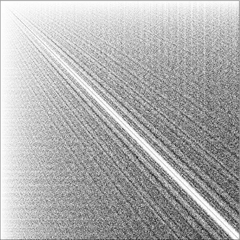
Figure 2: Density plot of the matrix $Q_{ij}$ for the range $i,j=1\cdots N$ for $N=1000$. $i=j=1$ is in the top left corner. The domain used was a smooth deformation of the circle, in $d=2$, with Dirichlet boundary conditions; the classical flow is almost completely ergodic. By Weyl’s Law the energy level density is constant, therefore the axes can equally well be thought of as $E_{i}$ and $E_{j}$. Eigenfunctions were calculated using the scaling method ([5], Appendix B). Dark indicates large magnitude values of $Q$, white indicates zero. The visible white band (very small values) with growing width $E^{1/2}$ around the diagonal (dark line) shows the quasi-orthogonality property special to the choice of (4). The visibly ‘banded’ structure is discussed in Section 3.1.

This Corollary is a stronger form of a conjecture first made (we believe) by Vergini-Saraceno (see Appendix of [25]). Making use of an identity equating (10) with $(E_{j}-E_{i})\langle\phi_{i},{\mathbf{r}}\cdot\nabla\phi_{j}\rangle_{\Omega}$ for $i\neq j$ (e.g. see [4] Eq.(H.25)), they suggested that off-diagonal elements vanish linearly as $|E_{i}-E_{j}|$. We now know by Theorem 1 that the vanishing is of higher order, namely as $(E_{i}-E_{j})^{2}$. Understanding this order of vanishing is important for understanding the accuracy of the numerical ‘scaling method’, as we will discuss below.

For domains whose geodesic flow (equivalently, classical dynamics) is ergodic, a semiclassical argument (of the type we will discuss in Section 3.1), more powerful than that of Vergini-Saraceno, was developed by Cohen, Heller and this author. This predicted the $(E_{i}-E_{j})^{2}$ factor appearing in (7), and showed excellent agreement with numerical studies [3, 4]. The argument involved evaluation along classical trajectories of a non-smooth operator which ‘lives’ (is a delta-function) on the boundary and possesses a ‘strength’ $D({\mathbf{s}})$ (see [4]). For the case $D({\mathbf{s}})=r_{n}$, corresponding to dilation of the billiard, the operator can be shown to be an exact second time-derivative of a bounded function. As a result its power-spectrum vanishes at zero frequency and this, via the semiclassical argument, is seen to be the cause of the $(E_{i}-E_{j})^{2}$ factor. However this explanation has problems: i) it relies on a semiclassical argument not yet proven to hold for all matrix elements (see Section 3.1), ii) the semiclassical argument is not known to be valid for such singular operators living on the boundary, and iii) only ergodic domains can be handled.

Corollary 1.2 provides proof of Dirichlet quasi-orthogonality without resort to any assumptions about the shape or ergodicity of the domain. In effect the identity in Lemma 1.1 below bypasses the two classical time-derivatives, and the semiclassical argument, by directly accounting for the $(E_{i}-E_{j})^{2}$ factor. Thus quasi-orthogonality is seen to be a result independent of any semiclassical or quantum ergodic assumptions. What we will be left with is consideration of matrix elements of the operator $r^{2}$, which is a smooth and bounded function of space. Bounds on these matrix elements are much easier to find than in the case of matrix elements involving boundary information. Lemma 1.1 relies on overlap identities which follow from the Divergence Theorem alone; these identities are derived in the Appendix using a symbolic matrix technique. Theorem 1 will then follow from an elementary bound on matrix elements. The possibility of considering boundary quasi-orthogonality with general boundary conditions, as we do with Theorem 1, is to our knowledge new.

In terms of applications, Dirichlet quasi-orthogonality (Corollary 1.2) is a key component of the ‘scaling method’ invented by Vergini-Saraceno [25] (see [4, 6], and Appendix B of the companion paper [5] for review), a very efficient method for the numerical solution of the Dirichlet eigenproblem in strictly star-shaped domains ($r_{n}>0$). This method has enabled large-scale studies of eigenfunctions at extremely high $E$ in $d=2$ [24, 5] and $d=3$ [20], where it outperforms all other known methods by a factor of typically $10^{3}$. The role played by the matrix $Q$ is as follows: The small size of off-diagonal elements of $Q$ near the diagonal means that a set of the domain’s Dirichlet eigenfunctions approximately diagonalize two certain quadratic forms (see Appendix B of [5]). The numerical method involves simultaneous diagonalization of these two quadratic forms, in order to compute a large number of approximate domain eigenfunctions at once. The error in the approximation, and therefore in the functions found by the method, depends on among other things the order of vanishing of $Q$ as one approaches the diagonal. Thus our work finally places this important method on a more rigorous footing, one which, despite its successful use, it has not yet had. In particular its success in domains with mixed dynamics (divided phase space), quasi-integrable, or integrable dynamics is now no longer mysterious. Moreover the generality of (2) and (3) opens up the possibility of extending the scaling method to solve eigenproblems with more general boundary conditions.

As another application, in the Dirichlet case (6) becomes

$$\oint_{\Gamma}\!r_{n}(\partial_{n}\phi_{i})^{2}\,{dA}\;=\;2E_{i},\qquad\mbox{for all }i\geq 1,$$ (11)

a result first found by Rellich [21] and independently by Berry-Wilkinson [8]. (Other more simple derivations have recently been found [3, 4, 13]). This formula is useful numerically because it enables Dirichlet eigenfunctions to be correctly normalized using boundary information alone. For general boundary conditions (6) reads

$$\oint_{\Gamma}\!(d-2)\phi_{i}\partial_{n}\phi_{i}+r_{n}\left(E_{i}\phi_{i}^{2}-|\nabla\phi_{i}|^{2}\right)+2\partial_{r}\phi_{i}\partial_{n}\phi_{i}\,{dA}=2E_{i},\quad\mbox{for all }i\geq 1,$$ (12)

a normalization formula involving boundary values and first derivatives alone, which we have not found in the literature. By contrast, the general boundary condition formula of Boasman for $d=2$ (Appendix D of [9]) requires second derivatives, a numerically more complicated demand.

Finally we note some other recent work on eigenfunctions on the boundary. In the Dirichlet case the asymptotic completeness in $C^{\infty}(\Gamma)$ of the boundary functions has been shown (this holds even when restricted to an energy window), and the curvature correction to their local intensity derived and tested numerically [2]. A version of the Quantum Ergodicity Theorem [23] for boundary functions has been proved in piecewise-smooth domains [14]. We note that boundary normalization formulae such as (11) break down for general Riemannian manifolds with boundary [13], so we expect that our results are specific to the Euclidean case.

The remainder of the paper is structured as follows. In Section 2 we prove Theorem 1, and give a recipe for translating the origin in such a way that the bound $C$ achieves its minimum value $C_{0}$. In Section 3 we review some semiclassical results on the size of matrix elements of well-behaved operators as $E\rightarrow\infty$. Applying them to the operator $r^{2}$, for domains with ergodic flow we improve somewhat the convergence rate in part 2) of Corollary 1.1. However, in contrast to our main results, this improved ergodic statement is not proved to hold for every single element $i,j$. We will also briefly mention expected behaviour for domains with integrable and mixed flow. The Appendix contains a detailed account of a general symbolic matrix procedure used to derive certain identies used in the proof in Section 2.

Acknowledgements. This work could not have been possible without interactions with and important feedback from Percy Deift, Fanghua Lin, Peter Sarnak, Maciej Zworski, Kevin Lin, Doron Cohen and Eduardo Vergini. The boundary formulae of Appendix A originated in work with Michael Haggerty and Eric Heller. The author is supported by the Courant Institute at New York University.

2 Proof of Theorem 1

Theorem 1 hinges on the following identity between elements of the matrix $Q$ and matrix elements of the function $r^{2}$ over the domain.

Lemma 1.1

Let $Q$ be the matrix defined by (4) and (5), with Laplace eigenfunctions defined by (1), (2) and (3). Then,

$$Q_{ij}\;=\;2E_{i}\delta_{ij}\;+\;\frac{{\epsilon_{ij}}^{2}}{4}{\langle\phi_{i},r^{2}\phi_{j}\rangle_{\Omega}},\qquad\mbox{for all }i,j\geq 1,$$ (13)

where ${\epsilon_{ij}}\equiv E_{i}-E_{j}$ is the difference in energies.

Notice that in (13) the first (resp. second) term contributes only on (resp. off) the diagonal.

Proof. Consider functions $u$ and $v$, defined with their derivatives on $\overline{\Omega}$, and each satisfying the Helmholtz equation, namely,

$$-\Delta u = E_{u}u,$$

$$-\Delta v = E_{v}v,$$ (14)

everywhere in $\Omega$. The functions need satisfy no particular boundary conditions on $\Gamma$. There are two cases which are handled separately: the energies $E_{u}$ and $E_{v}$ are either equal or unequal. Examining first the equal-energy case $E_{u}=E_{v}=E$, in the Appendix we derive the identity (see (36)),

$${\langle u,v\rangle_{\Omega}}\;=\;\frac{1}{2E}\oint_{\Gamma}\!\frac{d-2}{2}(u_{n}v+v_{n}u)+r_{n}\left(Euv-\nabla u\cdot\nabla v\right)+u_{r}v_{n}+v_{r}u_{n}\,{dA}.$$ (15)

This identity is a consequence of the Divergence Theorem applied to various combinations of the functions $u$ and $v$ and their first derivatives. Comparing this with (4) gives

$${\langle u,v\rangle_{\Omega}}\;=\frac{1}{2E}q(u,v;2E).$$ (16)

Substituting $u=\phi_{i}$ and $v=\phi_{j}$ and using the (5) and orthonormality on the domain gives,

$$Q_{ij}\;=\;2E_{i}\delta_{ij},\qquad\mbox{for}\;E_{i}=E_{j}.$$ (17)

This covers both the diagonal element case $i=j$ and the degenerate case where $i\neq j$ but $E_{i}=E_{j}$.

Now examining the case $E_{u}\neq E_{v}$, in the Appendix we derive the identity (equivalent to (33)),

$$\frac{\epsilon^{2}}{4}{\langle u,r^{2}v\rangle_{\Omega}}\;=\;\oint_{\Gamma}\!\frac{d-2}{2}(u_{n}v+v_{n}u)+\left(\frac{{\cal E}}{\epsilon}-\frac{\epsilon}{4}r^{2}\right)(u_{n}v-v_{n}u)\\ +r_{n}\left(\frac{{\cal E}}{2}uv-\nabla u\cdot\nabla v\right)+u_{r}v_{n}+v_{r}u_{n}\,{dA},$$ (18)

where the energy difference is $\epsilon\equiv E_{u}-E_{v}$ and the sum ${\cal E}\equiv E_{u}+E_{v}$. Applying self-adjoint boundary conditions (2) and (3) causes the term anti-symmetric in $u$ and $v$ to vanish identically on the boundary, leaving

$$\frac{\epsilon^{2}}{4}{\langle u,r^{2}v\rangle_{\Omega}}\;=\;q(u,v;\,E_{u}+E_{v}).$$ (19)

Substituting $u=\phi_{i}$ and $v=\phi_{j}$ and using (5) gives

$$Q_{ij}\;=\;\frac{{\epsilon_{ij}}^{2}}{4}{\langle\phi_{i},r^{2}\phi_{j}\rangle_{\Omega}}\qquad\mbox{for}\;E_{i}\neq E_{j}.$$ (20)

The two cases—equal energy (17) and differing energy (20)—can be summarized by the one identity (13). $\square$

We now see that the particular form (4) of $q$ results from a relatively complicated sequence of manipulations detailed in the Appendix. Lemma 1.1 has reduced the question of quasi-orthogonality to one of the size of the matrix elements ${\langle\phi_{i},r^{2}\phi_{j}\rangle_{\Omega}}$. Now the diagonal elements ${\langle\phi_{i},r^{2}\phi_{i}\rangle_{\Omega}}$ are trivially bounded by

$$\int_{\Omega}\!r^{2}\phi_{i}^{2}\,{dV}\;\leq\;R^{2}\int_{\Omega}\!\phi_{i}^{2}\,{dV}\;=\;R^{2},$$ (21)

where ${dV}$ is the volume element, and the maximum radius from the origin attained by the domain is

$$R\;\equiv\;\max_{{\mathbf{r}}\in\Gamma}|{\mathbf{r}}|.$$ (22)

Then by Cauchy-Schwarz we have off-diagonal matrix elements bounded by the same constant,

$$|{\langle\phi_{i},r^{2}\phi_{j}\rangle_{\Omega}}|\;\leq\;|{\langle\phi_{i},r^{2}\phi_{i}\rangle_{\Omega}}|^{1/2}|{\langle\phi_{j},r^{2}\phi_{j}\rangle_{\Omega}}|^{1/2}\;\leq\;R^{2}.$$ (23)

Substituting this into (13) completes the proof of Theorem 1, with the constant being $C=R^{2}/4$. $\square$

Clearly the eigenproblem (1), (2) and (3) is translationally invariant, that is, $\{E_{i}\}$ and $\{\phi_{i}\}$ are independent of the choice of origin for our coordinate ${\mathbf{r}}$. It follows from (6) that the diagonal elements of $Q$ are also translationally invariant; however the off-diagonal elements of $Q$ are not. Let us assume our task is, given a domain $\Omega$ of particular shape, to find the boundary form given by (4) for which the constant in (7) can be chosen to be smallest. We are free to translate the origin to achieve this goal. Clearly the minimum $C$ is given by $C_{0}=R_{0}^{2}/4$, where $R_{0}$ is the radius of the smallest circle (generally, ball in $\mathbb{R}^{d}$) enclosing $\Omega$. This is the escribed circle (or ball); see Fig. 1b. The optimal choice of origin is the center of this circle, ${\mathbf{r}}_{0}$. We note that any choice for the origin need not fall inside $\Omega$ and that none of the results given in this paper depend on whether it does or not. (This contrasts the scaling method, for which it is believed that the domain must be strictly star-shaped with respect to the origin).

3 Semiclassical estimates

The power of Lemma 1.1 is that it has reduced the quasi-orthogonality question to one of the size of matrix elements of a bounded operator $r^{2}$, in such a way that a trivial bound on ${\langle\phi_{i},r^{2}\phi_{j}\rangle_{\Omega}}$ is adequate to prove Theorem 1. Can we go beyond this bound? Estimating matrix elements semiclassically (at large $E$) has been a major theme in both the physics and mathematics communities, and remains an active area of research. We will now draw on their results. We emphasize that to prove Theorem 1, semiclassical results have not been used.

Depending on the domain (‘billiard’) shape, the geodesic flow on $\Omega\times S^{d-1}$, that is, the classical motion of a trapped point particle undergoing elastic reflections from $\Gamma$, falls into three broad categories: ergodic, integrable, and mixed [18]. This has consequences for the Laplace eigenfunctions which have been a major theme in ‘quantum chaos’ [16, 22].

3.1 Ergodic domains

In the ergodic case, the Quantum Ergodicity Theorem [23] (QET) has been proved, stating that asymptotically ($E\rightarrow\infty$) all but a set of measure zero of the eigenfunctions become spatially equidistributed across the domain. Thus almost all diagonal elements ${\langle\phi_{i},r^{2}\phi_{i}\rangle_{\Omega}}$ tend to the classical average $\int_{\Omega}r^{2}\,{dV}/\mbox{vol($\Omega$)}$. However this is not of direct use since it is only off-diagonal elements of $r^{2}$ that play a role in Lemma 1.1. Assuming a statistical model in which eigenfunctions behave like uncorrelated random-waves [7], off-diagonal elements are expected to be Gaussian distributed with zero mean; this has indeed been verified numerically [1, 19].

The remaining issue is their variance. This issue is discussed in much more detail in [5] but we provide a summary here. Almost all off-diagonal elements have been proven to vanish asymptotically [27] implying that the variance must vanish. However, the random-wave prediction for variance size is poor [1, 3, 5] since it cannot account for variance changing as a function of energy difference, that is, a ‘banded structure’ to the matrix. The banded matrix structure in the case of an ergodic domain is shown in Fig. 2. The semiclassical sum rule of Feingold-Peres [12, 11] (FP) has proven much more successful in predicting numerically observed variance [12, 11, 1, 19, 3], including the banded structure. There is numerical evidence [5] that it is asymptotically correct in billiard systems, but that convergence is quite slow. The band profile of the matrix elements of an operator $\hat{A}$, that is, variance as a function of energy difference, is related to $\tilde{C}_{A}(\omega)$, the Fourier transform of the auto-correlation of the corresponding classical operator under the (unit-speed) classical flow. FP states that for operators $\hat{A}$ whose classical counterparts are well-behaved in phase-space,

$$\mbox{var}\left[\langle\phi_{i},\hat{A}\phi_{j}\rangle_{\Omega}\right]\;\rightarrow\;\frac{\tilde{C}_{A}(\omega_{ij})}{\mbox{vol($\Omega$)}}E^{-1/2}\qquad\mbox{for }E_{i}\approx E_{j}\approx E\rightarrow\infty,$$ (24)

where the wavenumber difference is $\omega_{ij}\equiv E_{i}^{1/2}-E_{j}^{1/2}$. The sense in which we use ‘variance’ here is the variance of a large sample of matrix elements which share similar values of $\omega_{ij}$ and fall within a classically-small energy range. Thus, we are measuring variance within a small ‘patch’ of the matrix $\langle\phi_{i},\hat{A}\phi_{j}\rangle_{\Omega}$. As with Corollary 1.1, we now restrict ourselves to the energy window $\epsilon_{0}=o(E^{1/2})$, within which $\omega_{ij}\rightarrow 0$ as $E\rightarrow\infty$ (corresponding classically to taking the zero-frequency limit). Choosing $\hat{A}=r^{2}$, then (24) and Lemma 1.1 gives matrix element size

$$|Q_{ij}|\;\approx\;\left(\mbox{var}\left[Q_{ij}\right]\right)^{1/2}\;\rightarrow\;\left(\frac{\tilde{C}_{r^{2}}(0)}{4\mbox{vol($\Omega$)}}\right)^{1/2}\!\!\!E^{-1/4}\,(E_{i}-E_{j})^{2},$$ (25)

which holds for nearly all off-diagonal elements, and should be compared to the hard bound (7). The domain-dependent constant $\tilde{C}_{r^{2}}(0)$ can be estimated numerically via trajectory simulations; we do not know if it is minimized by the optimal choice of origin ${\mathbf{r}}_{0}$ derived in Section 2. Thus in part 2) of Corollary 1.1, we can improve the bound to $c_{\beta}E^{2\beta-5/4}$. For $\beta=0$ (constant energy difference), the convergence rate then improves somewhat from $E^{-1}$ to $E^{-5/4}$. Note that this result is equivalent to that of [3, 4], but because $r^{2}$ is a smooth rather than singular function the approach presented here stands on more solid foundations, as discussed in Section 1. However, FP is not proven to hold for every single matrix element: there may exist an exceptional set (analogous to the diagonal case) which fails to converge as above. Theorem 1 remains the only proven bound on $Q$ known to us.

It is worth pointing out that ergodicity and the FP sum rule, if it were valid for singular functions (as it empirically appears to be [3]), would imply a weaker form of asymptotic quasi-orthogonality, regardless of the form of $q$. That is, Corollary 1.1 would hold even for generic boundary forms with terms similar to those in (4) but lacking their particular cancellations, for almost all off-diagonal elements, independent of $E_{i}-E_{j}$, but with the much slower convergence rate $\sim cE^{-1/4}$. In the case of Dirichlet boundary conditions, this would correspond to choosing a generic weight function $D({\mathbf{s}})$ in place of $r_{n}$ in (10).

When the ergodic flow furthermore is Anosov (uniformly hyperbolic), a stronger version of QET has been conjectured [22], which lifts the requirement that a zero-density set be excluded. This is known as Quantum Unique Ergodicity (QUE), and currently remains unproven in Euclidean domains, although good numerical evidence exists when $d=2$ [5]. Since QUE can be extended to off-diagonal elements [28], if proven, QUE would enable the improved bounds (25) to be claimed for every single off-diagonal element in these classes of domains.

If the flow contains orbits with zero Lyapunov exponent (‘bouncing ball modes’), classical autocorrelations generally have a power-law rather than exponential tail, thus $\tilde{C}_{A}(\omega)$ diverges as $\omega\rightarrow 0$, and (25) is undefined. In this case FP must be modified, and to our knowledge only the diagonal variance has been carefully studied theoretically [11].

3.2 Integrable and mixed domains

Finally we briefly mention some of what is known about the behaviour of matrix elements in systems with other categories of classical dynamics, and speculate on consequences for the rate of convergence in Corollary 1.1.

If the classical dynamics is integrable, then eigenfunctions are regular, with Wigner functions concentrating around $d$-dimensional classical invariant tori in phase space [18, 16]. Each eigenfunction possesses a well-defined set of quantum number labels ${\mathbf{p}}\in\mathbb{Z}^{d}$; values of ${\mathbf{r}}$ tend to be uncorrelated as a function of level number. Much less has been said about off-diagonal matrix elements in this case. In smooth Hamiltonian systems matrix elements between levels labelled by ${\mathbf{p}}$ and ${\mathbf{q}}$ are expected to die like $\exp(-c|{\mathbf{p}}-{\mathbf{q}}|)$, for a generic smooth operator. Thus most off-diagonal elements are exponentially small (the so-called ‘selection rules’ [16, 17]), but a few may be large, that is, of the same order as diagonal elements. However, because our domain has a hard boundary condition, it is easy to estimate (by analogy with the $d=1$ case) that generic matrix elements die algebraically with $|{\mathbf{p}}-{\mathbf{q}}|)$. Thus we still expect most off-diagonal elements to be small. This has been observed numerically in billiard systems [19, 17]. Thus, we expect that convergence to quasi-orthogonality will be much more rapid, for the majority of matrix elements, than for the ergodic case. In general, it is hard to say more. It would be interesting to see if integrable examples can be found where ${\langle\phi_{i},r^{2}\phi_{j}\rangle_{\Omega}}$ approaches $R^{2}$ as $E\rightarrow\infty$; this would prove that Theorem 1 is sharp, with $C=R^{2}/4$.

A generic domain has mixed dynamics, and eigenfunctions either occupy ergodic components of phase space, or lie on integrable tori. Matrix elements involving energy levels lying in different components are therefore expected to be very small. This has been verified numerically in some smooth Hamiltonian systems [10], but no study in billiards is known. There is much opportunity for numerical study in such billiard systems.

Appendix A: Boundary identities for matrix elements

We present and apply a novel general procedure for deriving identities which express certain bilinear forms over a domain, involving solutions to the Helmholtz equation purely in terms of bilinear forms on the boundary. Given a bounded open domain $\Omega\subset\mathbb{R}^{d}$, $d\geq 2$, let the fields $u({\mathbf{r}})$, $v({\mathbf{r}})$ be regular solutions of (14) with energies $E_{u}$ and $E_{v}$ respectively, everywhere in $\Omega$. We envisage $\Gamma$ being the union of a finite number of smooth curves (surfaces), however the broader condition that $\Omega$ be Lipschitz is sufficient. Crucially, we do not require any particular boundary conditions to be satisfied by $u$, $v$ on $\Gamma$. We will make use of the Divergence Theorem applied to vector fields which are bilinear combinations of $u,v$ and their first derivatives; thus $u$ and $v$ need only be sufficiently regular that the Divergence Theorem can be applied to such a vector field. These conditions on vector fields are quite broad [15]. We believe that the conditions laid out at the beginning of this paper are sufficient to ensure that $u$ or $v$ can be set to equal any eigenfunction $\phi_{i}$ and still have the Divergence Theorem apply. We will express

$$\langle u,\hat{H}v\rangle_{\Omega}:=\int_{\Omega}\!u\hat{H}v\,{dV},$$ (26)

${dV}$ being the volume element in $\mathbb{R}^{d}$, in terms of boundary integrals involving values and first derivatives of $u$ and $v$, for the operator choices $\hat{H}=1$ and $\hat{H}={\mathbf{r}}\cdot{\mathbf{r}}:=r^{2}$. We will consider both the cases $E_{u}\neq E_{v}$ and $E_{u}=E_{v}$.

Consider functions on $\Omega$ that are built from bilinear forms in $u,v$ and their spatial derivatives. We restrict attention to such functions that are either scalar fields or vector fields. The key is to select a set of scalars $\{q_{\beta}\}$, $\beta=1,2\ldots{N_{q}}$, and a set of vectors $\{{\mathbf{p}}_{\alpha}\}$, $\alpha=1,2\ldots{N_{{\mathbf{p}}}}$, such that the divergence of each vector field can be written as a (location-independent) linear combination of the scalar fields. Applying the Divergence Theorem turns these into relations between boundary and volume integrals. The coefficients form a matrix, which can be handled symbolically to express volume integrals as linear combinations of boundary integrals. We note that the idea of inverting such a coefficient matrix originated in unpublished work of Michael Haggerty (see Appendix H of [4]), however here we extend the idea and explore a larger set of vector and scalar terms.

order	$r^{0}$	$r^{1}$	$r^{2}$
$\partial^{0}$	$uv$	—	$\overset{\mbox{\raisebox{-1.29167pt}[3.01385pt][0.0pt]{$\scriptstyle\smallfrown$}}}{rr}uv$
$\partial^{1}$	$\overset{\mbox{\raisebox{-1.29167pt}[3.01385pt][0.0pt]{$\scriptstyle\smallfrown$}}}{uv}$	$\overset{\mbox{\raisebox{-1.29167pt}[3.01385pt][0.0pt]{$\scriptstyle\smallfrown$}}}{ru}v$, $\leftrightarrow$	$\overset{\mbox{\raisebox{-1.29167pt}[3.01385pt][0.0pt]{$\scriptstyle\smallfrown$}}}{rr}\overset{\mbox{\raisebox{-1.29167pt}[3.01385pt][0.0pt]{$\scriptstyle\smallfrown$}}}{uv}$, $\overset{\mbox{\raisebox{-1.29167pt}[3.01385pt][0.0pt]{$\scriptstyle\smallfrown$}}}{ru}\overset{\mbox{\raisebox{-1.29167pt}[3.01385pt][0.0pt]{$\scriptstyle\smallfrown$}}}{rv}$
$\partial^{2}$	$\overset{\mbox{\raisebox{-1.29167pt}[3.01385pt][0.0pt]{$\,\scriptstyle\smallfrown\mkern-16.5mu\displaystyle\smallfrown$}}}{uv}$	$\overset{\mbox{\raisebox{-1.29167pt}[3.01385pt][0.0pt]{$\scriptstyle\smallfrown\scriptstyle\smallfrown$}}}{ruv}$, $\leftrightarrow$	$\overset{\mbox{\raisebox{-1.29167pt}[3.01385pt][0.0pt]{$\scriptstyle\smallfrown$}}}{rr}\overset{\mbox{\raisebox{-1.29167pt}[3.01385pt][0.0pt]{$\,\scriptstyle\smallfrown\mkern-16.5mu\displaystyle\smallfrown$}}}{uv}$, $\overset{\mbox{\raisebox{-1.29167pt}[3.01385pt][0.0pt]{$\scriptstyle\smallfrown\scriptstyle\smallfrown\scriptstyle\smallfrown$}}}{ruvr}$, $\overset{\mbox{\raisebox{-1.29167pt}[3.01385pt][0.0pt]{$\scriptstyle\smallfrown\scriptstyle\smallfrown$}}}{rur}v$, $\leftrightarrow$

Table 1: Lowest order scalar diagrams (‘molecules’) from which the set of functions $\{q_{\beta}\}$ was chosen. An order of $\partial^{m}$ means that $m$ is the highest order derivative of $u$ or $v$. The symbol $\leftrightarrow$ means a repetition of the previous diagram but with $u$ and $v$ swapped. See text for further explanation.

order	$r^{0}$	$r^{1}$	$r^{2}$
$\partial^{0}$	—	$\overset{\mbox{\raisebox{-1.29167pt}[3.01385pt][0.0pt]{$.$}}}{r}uv$	—
$\partial^{1}$	$\overset{\mbox{\raisebox{-1.29167pt}[3.01385pt][0.0pt]{$.$}}}{u}v$, $\leftrightarrow$	$\overset{\mbox{\raisebox{-1.29167pt}[3.01385pt][0.0pt]{$.$}}}{r}\overset{\mbox{\raisebox{-1.29167pt}[3.01385pt][0.0pt]{$\scriptstyle\smallfrown$}}}{uv}$, $\overset{\mbox{\raisebox{-1.29167pt}[3.01385pt][0.0pt]{$\scriptstyle\smallfrown$}}}{ru}\overset{\mbox{\raisebox{-1.29167pt}[3.01385pt][0.0pt]{$.$}}}{v}$, $\leftrightarrow$	$\overset{\mbox{\raisebox{-1.29167pt}[3.01385pt][0.0pt]{$\scriptstyle\smallfrown$}}}{rr}\overset{\mbox{\raisebox{-1.29167pt}[3.01385pt][0.0pt]{$.$}}}{u}v$, $\leftrightarrow$, $\overset{\mbox{\raisebox{-1.29167pt}[3.01385pt][0.0pt]{$.$}}}{r}\overset{\mbox{\raisebox{-1.29167pt}[3.01385pt][0.0pt]{$\scriptstyle\smallfrown$}}}{ru}v$, $\leftrightarrow$

Table 2: Lowest order vector diagrams (‘radicals’) from which the set of functions $\{{\mathbf{p}}_{\alpha}\}$ was chosen. See Table 1 caption for explanation.

To build the functions we use the following objects: the fields $u,v$, their gradients $u_{i}:=\partial_{i}u$ and higher derivative tensors $u_{ij}:=\partial_{i}\partial_{j}u$, etc, and polynomials in the coordinates $r_{i}$ which transform as scalars, vectors, tensors, etc. It is possible to enumerate systematically, using diagrams, the hierarchy of such combinations with overall scalar or vector character. Diagrams also greatly ease the algebra in taking the divergence of the vector functions (we apply the rules by hand, but automating them would not be hard).

We have found the following scheme very useful. A combination of overall scalar character is represented by a ‘molecule’ (or a disconnected collection of molecules) built from ‘atoms’ connected by ‘bonds’. Each atom can be either $r$, $u$, or $v$. A bond carries summation over a spatial index, for instance $i$; when a bond terminates at $u$ or $v$ this corresponds to a derivative $\partial_{i}$, whereas termination at $r$ corresponds simply to $r_{i}$. Thus $u$ and $v$ may carry $0,1,\ldots\infty$ bonds whereas each $r$ must carry exactly 1. See Table 1 for the few lowest-order scalar functions. For example, $\overset{\mbox{\raisebox{-1.29167pt}[3.01385pt][0.0pt]{$\scriptstyle\smallfrown\scriptstyle\smallfrown$}}}{ruv}$ represents $\sum_{i=1}^{d}\sum_{j=1}^{d}r_{i}u_{ij}v_{j}$. From now on summation over repeated indices is implied.

A combination of overall vector character is similar except it has exactly one ‘dangling bond’, represented by a dot (we could think of it as a ‘radical’). Taking the divergence of a vector function corresponds to first summing the molecules resulting from connecting the dangling bond to each of the atoms in turn (including the one from which it originates). The molecules produced are not necessarily valid, so the following three ‘reaction’ rules need to be applied repeatedly until each molecule becomes valid:

1. $\overset{\mbox{\raisebox{-1.29167pt}[3.01385pt][0.0pt]{$\scriptscriptstyle\cap$}}}{u}\rightarrow-E_{u}u$. That is, self-bonds to atoms $u$ or $v$ vanish and are replaced by the scalar multiplier $-E_{u}$ or $-E_{v}$ respectively.

2. $\overset{\mbox{\raisebox{-1.29167pt}[3.01385pt][0.0pt]{$\scriptscriptstyle\cap$}}}{r}\rightarrow d$. That is, any $r$ bonded to itself vanishes along with the bond, and is replaced by the scalar multiplier $d$.

3. $\overset{\mbox{\raisebox{-1.29167pt}[3.01385pt][0.0pt]{$\scriptstyle\smallfrown\scriptstyle\smallfrown$}}}{r}\rightarrow\overset{\mbox{\raisebox{-1.29167pt}[3.01385pt][0.0pt]{$\scriptstyle\smallfrown$}}}{\rule{0.0pt}{4.30554pt}}$. That is, any $r$ with two bonds (not covered by the previous rule) vanishes, and the resulting dangling ends connect to form a single bond.

It can be easily verified that this procedure is equivalent to taking the divergence of any given vector field. For example, the divergence of $r^{2}u_{i}v$ is computed as follows,

$$\overset{\mbox{\raisebox{-1.29167pt}[3.01385pt][0.0pt]{$\scriptstyle\smallfrown$}}}{rr}\overset{\mbox{\raisebox{-1.29167pt}[3.01385pt][0.0pt]{$.$}}}{u}v \rightarrow 2\overset{\mbox{\raisebox{-1.29167pt}[3.01385pt][0.0pt]{$\scriptstyle\smallfrown\scriptstyle\smallfrown$}}}{rru}v+\overset{\mbox{\raisebox{-1.29167pt}[3.01385pt][0.0pt]{$\scriptstyle\smallfrown$}}}{rr}\overset{\mbox{\raisebox{-1.29167pt}[3.01385pt][0.0pt]{$\scriptscriptstyle\cap$}}}{u}v+\overset{\mbox{\raisebox{-1.29167pt}[3.01385pt][0.0pt]{$\scriptstyle\smallfrown$}}}{rr}\overset{\mbox{\raisebox{-1.29167pt}[3.01385pt][0.0pt]{$\scriptstyle\smallfrown$}}}{uv}$$ (27)

$$\stackrel{{\scriptstyle{\mbox{\tiny rules}}}}{{\rightarrow}} 2\overset{\mbox{\raisebox{-1.29167pt}[3.01385pt][0.0pt]{$\scriptstyle\smallfrown$}}}{ru}v-E_{u}\overset{\mbox{\raisebox{-1.29167pt}[3.01385pt][0.0pt]{$\scriptstyle\smallfrown$}}}{rr}uv+\overset{\mbox{\raisebox{-1.29167pt}[3.01385pt][0.0pt]{$\scriptstyle\smallfrown$}}}{rr}\overset{\mbox{\raisebox{-1.29167pt}[3.01385pt][0.0pt]{$\scriptstyle\smallfrown$}}}{uv},$$

thus the answer is $2r_{i}u_{i}v-E_{u}r^{2}uv+r^{2}u_{i}v_{i}$, evident as row $\alpha=7$ of the matrix equation (28) below.

Using this technique we have calculated the divergence of the simplest 25 or so vectors, which results in a similar number of scalars. For the goal at hand we have eventually found the following vector subset of size ${N_{{\mathbf{p}}}}=8$ and scalar subset of size ${N_{q}}=8$ to be minimally sufficient,

$$\partial_{i}\left(\begin{array}[]{c}u_{i}v\\ v_{i}u\\ r_{i}uv\\ r_{i}u_{j}v_{j}\\ r_{j}u_{j}v_{i}\\ r_{j}v_{j}u_{i}\\ r^{2}u_{i}v\\ r^{2}v_{i}u\\ \end{array}\right)\;\;=\;\;\left(\begin{array}[]{cccccccc}-E_{u}&1&0&0&0&0&0&0\\ -E_{v}&1&0&0&0&0&0&0\\ d&0&1&1&0&0&0&0\\ 0&d&0&0&1&1&0&0\\ 0&1&-E_{v}&0&1&0&0&0\\ 0&1&0&-E_{u}&0&1&0&0\\ 0&0&2&0&0&0&-E_{u}&1\\ 0&0&0&2&0&0&-E_{v}&1\end{array}\right)\left(\begin{array}[]{c}uv\\ u_{i}v_{i}\\ r_{i}u_{i}v\\ r_{i}v_{i}u\\ r_{i}u_{ij}v_{j}\\ r_{i}v_{ij}u_{j}\\ r^{2}uv\\ r^{2}u_{i}v_{j}\end{array}\right).$$ (28)

This set of divergence relations can be more compactly written,

$$\nabla\cdot{\mathbf{p}}_{\alpha}\;=\;\sum_{\beta=1}^{{N_{q}}}{\cal M}_{\alpha\beta}\,q_{\beta},\qquad\alpha=1,2\ldots{N_{{\mathbf{p}}}}.$$ (29)

Integrating over $\Omega$ and applying the Divergence Theorem gives

$$\oint_{\Gamma}\!{\mathbf{n}}\cdot{\mathbf{p}}_{\alpha}{dA}\;=\;\sum_{\beta=1}^{{N_{q}}}{\cal M}_{\alpha\beta}\,\int_{\Omega}\!q_{\beta}\,{dV},\qquad\alpha=1,2\ldots{N_{{\mathbf{p}}}}.$$ (30)

We first consider the case $E_{u}\neq E_{v}$, for which the matrix ${\cal M}$ is invertible (in fact we chose the above set of vectors to make this so). Thus each volume integral appearing in (30) can be written purely in terms of boundary integrals,

$$\int_{\Omega}\!q_{\alpha}\,{dV}\;=\;\sum_{\beta=1}^{{N_{{\mathbf{p}}}}}\left({\cal M}^{-1}\right)_{\alpha\beta}\oint_{\Gamma}\!{\mathbf{n}}\cdot{\mathbf{p}}_{\beta}\,{dA}\qquad\alpha=1,2\ldots{N_{q}}.$$ (31)

A symbolic algebra package (Mathematica) was used to find ${\cal M}^{-1}$, which we need not write out in full here. Rather we use only select rows of ${\cal M}^{-1}$, that is, certain values of $\alpha$ in (31). For example, the $\alpha=1$ row of ${\cal M}^{-1}$ is $(1/(E_{u}-E_{v}),-1/(E_{u}-E_{v}),0,0,0,0,0,0)$, immediately gives the simple relation

$$\langle u,v\rangle_{\Omega_{A}}\;=\;\frac{1}{E_{u}-E_{v}}\oint_{\Gamma_{A}}\!(u{\mathbf{n}}\cdot\nabla v-v{\mathbf{n}}\cdot\nabla u)\;{dA},$$ (32)

well-known from Green’s Theorem. Choosing the $\alpha=7$ row gives, expressed in terms of $\epsilon:=E_{u}-E_{v}$ and ${\cal E}:=E_{u}+E_{v}$, the relation

$$\int_{\Omega}\!r^{2}uv\,{dV}\;=\;\frac{4}{\epsilon^{2}}\oint_{\Gamma}\!\frac{d-2}{2}(u_{n}v+v_{n}u)+\left(\frac{{\cal E}}{\epsilon}-\frac{\epsilon}{4}r^{2}\right)(u_{n}v-v_{n}u)\\ +r_{n}\left(\frac{{\cal E}}{2}uv-\nabla u\cdot\nabla v\right)+u_{r}v_{n}+v_{r}u_{n}\,{dA}.$$ (33)

In the particular case of Dirichlet boundary conditions on $\Gamma$, using $\nabla u={\mathbf{n}}u_{n}$, etc, this relation simplifies to

$$\int_{\Omega}\!r^{2}uv\,{dV}\;=\;\frac{4}{\epsilon^{2}}\oint_{\Gamma}\!r_{n}u_{n}v_{n}{dA},$$ (34)

a result we have not found in the literature.

We now consider $E_{u}=E_{v}=E$, in which case ${\cal M}$ is not invertible (its first two rows are identical). However $\int_{\Omega}q_{\alpha}\,{dV}$ can still be expressed as a linear combination of boundary integrals if the standard unit basis vector ${\mathbf{b}}^{(\alpha)}:=(0,\ldots,0,1,0,\ldots,0)\in\mathbb{R}^{N_{q}}$, which contains a 1 only in location $\alpha$, lies in $\mbox{Row}{\cal M}$. Since in our case $\mbox{Nul}{\cal M}$ contains the single vector $(0,0,0,0,0,0,1,E)$, this can be done for $\alpha\in[1,6]$. For each such $\alpha$, we can find the row coefficient vector ${\mathbf{x}}^{(\alpha)}\in\mathbb{R}^{N_{{\mathbf{p}}}}$ by solving the (consistent and in this case underdetermined) linear equation

$${\cal M}^{T}{\mathbf{x}}^{(\alpha)}\;=\;{\mathbf{b}}^{(\alpha)}.$$ (35)

We remind the reader that the coefficient vector spaces between which ${\cal M}^{T}$ transforms should not be confused with coordinate vectors in $\mathbb{R}^{d}$. The solution set of (35) is readily found with a symbolic algebra package. For the case $\alpha=1$ the resulting row coefficients give the identity

$$\int_{\Omega}\!uv\,{dV}\;=\;\frac{1}{2E}\oint_{\Gamma}\!\frac{d-2}{2}(u_{n}v+v_{n}u)+r_{n}\left(Euv-\nabla u\cdot\nabla v\right)+u_{r}v_{n}+v_{r}u_{n}\,{dA}.$$ (36)

where we have (arbitrarily) chosen to equalize the first two coefficients in order to make the $u{\leftrightarrow}v$ symmetry manifest. This identity involves no derivatives higher than the first, and to our knowledge is new. A similar identity for $d=2$ which required second derivatives, and is therefore more cumbersome, has already been found [9] (also see [4], Eq.(H.7)). In the particular case of Dirichlet boundary conditions (36) directly proves (11).

What could be gained by enlarging the function spaces beyond ${N_{{\mathbf{p}}}}=8$ and ${N_{q}}=8$ ? For both cases $E_{u}=E_{v}$ and $E_{u}\neq E_{v}$, the only criterion for being able to express a volume integral $\int_{\Omega}q_{\alpha}\,{dV}$ in terms of boundary integrals is that the unit vector ${\mathbf{b}}^{(\alpha)}$ lie in $\mbox{Row}{\cal M}$. This is equivalent to the consistency of (35). Invertibility of $\cal M$ is sufficient but not necessary. It is an open question whether, by including a growing set of vector functions $\{{\mathbf{p}}_{\beta}\}$ (Table 2 and its continuation), and necessarily the resulting growing set of scalars $\{q_{\alpha}\}$, that the row space of the resulting growing matrix $\cal M$ can be made to contain the unit vector ${\mathbf{b}}^{(\alpha)}$ for any desired $\alpha$.

Note that the methods of this appendix are probably not simply generalizable to Riemannian manifolds with boundary. The Euclidean boundary formula (11) is known to break down in a general manifold, and unit-normalized eigenfunctions with exponentially-small values and gradients everywhere on the boundary become possible [13]. This is associated with the existence of trapped geodesics. However for the constant-curvature case, it would be interesting to search for a generalization.

References

- [1] E. J. Austin and M. Wilkinson, “Distribution of matrix elements of a classicaly chaotic system”, Europhys. Lett. 20, 589–593 (1992).
- [2] A. Bäcker, S. Fürstberger, R. Schubert, and F. Steiner, “Behaviour of boundary functions for quantum billiards”, J. Phys. A 35, 10293–10310 (2002).
- [3] A. H. Barnett, D. Cohen, and E. J. Heller, Phys. Rev. Lett. 85, 1412 (2000).
- [4] A. H. Barnett, Ph. D. thesis, Harvard University, 2000.
- [5] A. H. Barnett, “Asymptotic rate of quantum ergodicity in chaotic Euclidean billiards”, submitted, Comm. Pure Appl. Math, math-ph/0512030
- [6] A. H. Barnett, “The scaling method for the Laplace eigenproblem”, in preparation.
- [7] M. V. Berry, “Regular and irregular semiclassical wavefunctions”, J. Phys. A 10 2083–91 (1977).
- [8] M. V. Berry and M. Wilkinson, Proc. R. Soc. London A 392, 15 (1984).
- [9] P. A. Boasman, “Semiclassical accuracy for billiards”, Nonlin. 7, 485–537 (1994).
- [10] D. Boosé and J. Main, “Distributions of transition matrix elements in classically mixed quantum systems”, Phys. Rev. E 60, 2813–44 (1999).
- [11] B. Eckhardt, S. Fishman, J. Keating, O. Agam, J. Main, and K. Müller, “Approach to ergodicity in quantum wave functions”, Phys. Rev. E 52, 5893–5903 (1995).
- [12] M. Feingold and A. Peres, “Distribution of matrix elements of chaotic systems”, Phys. Rev. A, 34, 591 (1986).
- [13] A. Hassell and T. Tao, “Upper and lower bounds for normal derivatives of Dirichlet eigenfunctions”, Math. Res. Lett. 9, 289–305 (2002).
- [14] A. Hassell and S. Zelditch, arXiv:math.SP/0211140 (2003).
- [15] O. D. Kellogg, Foundations of Potential Theory (Springer, 1929).
- [16] M. C. Gutzwiller, Chaos in Classical and Quantum Mechanics, (Springer, NY, 1990).
- [17] B. Mehlig, “Semiclassical analysis of response functions for integrable systems”, Phys. Rev. B 55, R10193–96 (1997).
- [18] E. Ott, Chaos in Dynamical Systems, 2nd Ed. (Cambridge, 2002).
- [19] T. Prosen and M. Robnik, “Distribution and fluctuation properties of transition probabilities in a system between integrability and chaos”, J. Phys. A 26, L319–L326 (1993); note Figs. 2 and 3 are mistakenly swapped.
- [20] T. Prosen, “Quantization of a generic chaotic 3D billiard with smooth boundary. I. Energy level statistics”, Phys. Lett. A 233, 323–331 (1997); T. Prosen, “Quantization of a generic chaotic 3D billiard with smooth boundary. II. Structure of high-lying eigenstates”, Phys. Lett. A 233, 332–342 (1997).
- [21] F. Rellich, “Darstellung der Eigenwerte von durch ein Randintegral”, Math. Z. 46, 635–36 (1940).
- [22] P. Sarnak, “Arithmetic quantum chaos”, The Schur lectures (Tel Aviv, 1992), Israel Math. Conf. Proc. 8, 183–236 (Bar-Ilan University, 1995).
- [23] A. I. Schnirelman, Usp. Mat. Nauk. 29, 181 (1974); Y. Colin de Verdière, “Ergodicité et fonctions propres du laplacien”, Comm. Math. Phys. 102 497 (1985); S. Zelditch, “Uniform distribution of eigenfunctions on compact hyperbolic surfaces”, Duke Math. J. 55, 919 (1987); S. Zelditch and M. Zworski, “Ergodicity of eigenfunctions for ergodic billiards”, Comm. Math. Phys., 175 673–682 (1996).
- [24] G. Veble, M. Robnik, and J. Liu, “Study of regular and irregular states in generic systems”, J. Phys. A 32, 6423–44 (1999); G. Casati and T. Prosen, “The quantum mechanics of chaotic billiards”, Physica D 131, 293–310 (1999); D. Cohen, A. H. Barnett, and E. J. Heller, “Parametric evolution for a deformed cavity”, Phys. Rev. E 63, 046207 (2001).
- [25] E. Vergini and M. Saraceno, Phys. Rev. E, 52, 2204 (1995); E. Vergini, Ph. D. thesis, Universidad de Buenos Aires, 1995.
- [26] M. Wilkinson, “A semiclassical sum rule for matrix elements of classically chaotic systems”, J. Phys. A 20, 2415–23 (1987).
- [27] S. Zelditch, “Quantum transition amplitudes for ergodic and for completely integrable systems”, J. Funct. Anal. 94, 415–436 (1990).
- [28] S. Zelditch, “Note on Quantum Unique Ergodicity”, to appear, Proc. AMS, math-ph/0301035 (2003).