Geometrically induced two-particle binding in a wave guide

Abstract.

For mathematical models of quantum wave guides we show that in some situations two interacting particles can be trapped more easily than a single particle. In particular, we give an example of a wave guide that can not bind a single particle, but does have a geometrically induced bound state for two bosons that attract each other via a harmonic potential. We also show that Neumann boundary conditions are ‘stickier’ for two interacting bosons than for a single one.

1. Introduction

Over the last two decades a considerable amount of research has been done on mathematical models for quantum wave guides (see e.g. [1, 4, 6, 7, 8, 9] and references therein). Typically a particle in such a structure is modelled by a Schrödinger operator on some tube-like domain in two or three dimensions. The main object of interest is the spectrum of these operators, and especially their low-lying eigenvalues which indicate the presence of bound states for the particle. Such trapped modes have been proven to exist, e.g., for tubes with local deformations, bends, or mixed boundary conditions. Much less is known though about the binding of several interacting particles in such settings [10, 11, 13]. In [10] Exner and Vugalter addressed the question how many fermions can be bound in a curved wave guide if they are non-interacting or if they interact via a repulsive electrostatic potential. It is clear that for these systems a smaller number of particles can be bound more easily than a higher number of particles. In the present article we consider the somewhat opposite case and show that under certain conditions two bosons with an attractive interaction can be bound more easily than one particle alone.

Our work is inspired by the analogous effect for Schrödinger operators in free space: Consider for a particle of mass $m$ the operator

$$H=-\frac{1}{2m}\Delta+V(x)$$

in $L^{2}(\mathbb{R}^{n})$ with a non-trivial, compactly supported and bounded potential $V\leq 0$. It is well known that for $n>2$ the attractive potential $V$ may be too weak to have bound states, i.e., $H$ may not have negative eigenvalues. If this is the case, the same potential may still give rise to bound states of a system of two particles that attract each other. This can be understood by physical intuition if one assumes that the two particles act in some sense like one particle of the double mass. After all, as far as the existence of eigenvalues is concerned, doubling the mass has the same effect as doubling the strength of the potential. In the present article we discuss whether an analogous effect can occur for purely geometrically induced bound states in wave guides.

More precisely, we describe a quantum mechanical particle in a wave guide by the Dirichlet Laplacian $-\Delta$ in $L^{2}(\Omega)$, where $\Omega$ is a straight strip or tube. The spectrum of this operator is purely continuous and contains every real number above some threshold, which is the lowest eigenvalue of the Laplace operator on the cross section of $\Omega$. It is known that geometrical perturbations like bending the tube or local deformations of the boundary can give rise to eigenvalues of $-\Delta$ below this threshold. In analogy to the case of the Schrödinger operator with a weak attractive potential, we ask the following question: Does a wave guide exist that doesn’t have a bound state for one particle, but that does have a bound state for a system of two interacting particles?

This question is not so easy to answer by physical intuition, because the existence or non-existence of geometrically induced bound states for one particle doesn’t depend on the mass of the particle in question. This means that the intuitive ‘double mass argument’ for two particles in an attractive potential doesn’t apply to this situation. Despite that, we will show in the following two sections that the answer to the question above is ‘yes’ by giving an appropriate example.

2. Two-particle bound states in deformed wave guides

We assume our wave guide to be the domain $\Omega\subset\mathbb{R}^{2}$ given by

$$\Omega=\{(x,y):|y|<f(x)\}$$

where

$$f(x)=\left\{\begin{array}[]{ll}\frac{1}{2}&\textmd{for }|x|>L/2,\cr\epsilon/2&\textmd{for }x=\pm\,L/2,\cr h/2&\textmd{for }|x|<L/2\end{array}\right.$$

with $L>0,h>1$ and $0<\epsilon<1$.

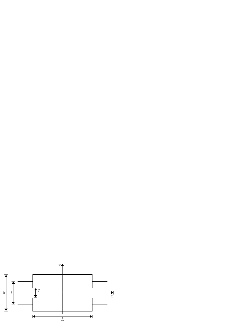
Figure 1. Sketch of the wave guide $\Omega$

We impose Dirichlet conditions on $\partial\Omega$, which includes the ‘barriers’ at $x=\pm L/2$. Our geometry can be interpreted as a cavity of length $L$ and width $h$ coupled weakly (if $\epsilon$ is small) to two semi-infinite straight wave guides. We choose to set $m=\frac{1}{2}$, such that the one-particle Hamiltonian is simply $H_{1}=-\Delta$. Then standard arguments imply that

$$\sigma_{\rm ess}(H_{1})=[\pi^{2},\infty).$$

Eigenvalues may occur depending on the choice of the parameters $L,h$ and $\epsilon$, but we will show:

Lemma 2.1.

If $L^{-2}+h^{-2}>1$ then for small enough $\epsilon$ there are no eigenvalues of $H_{1}$ below $\pi^{2}$, i.e., in this case the wave guide has no one-particle bound states.

On the other hand, we consider a system of two bosons of mass $m=\frac{1}{2}$, which interact via the harmonic potential

$$V=\alpha(x_{1}-x_{2})^{2}+\alpha(y_{1}-y_{2})^{2}.$$

Here $x_{i}$ and $y_{i}$ are the particle coordinates and $\alpha>0$ is the interaction strength. To define the self-adjoint Hamilton operator of the system we use the quadratic forms

$$h_{-\Delta}[\Psi] = \int_{\Omega\times\Omega}|\nabla\Psi|^{2}\,\mathrm{d}x\,\mathrm{d}y\quad\textmd{and}$$

$$h_{V}[\Psi] = \int_{\Omega\times\Omega}V|\Psi|^{2}\,\mathrm{d}x\,\mathrm{d}y,$$

both defined on $C_{0}^{\infty}(\Omega\times\Omega)$. Then by [2], Theorem 1.8.1, the sum of the two forms has a closure $h_{2}$ with

$$h_{2}[\Psi]=\overline{h_{-\Delta}}[\Psi]+\overline{h_{V}}[\Psi]$$

for all $\Psi$ in

(1) $${\rm Dom}(h_{2})=W_{0}^{1,2}(\Omega\times\Omega)\cap{\rm Dom}(\overline{h_{V}}).$$

The positive self-adjoint operator associated with $h_{2}$ is

$$H_{2}=-\partial_{x_{1}}^{2}-\partial_{y_{1}}^{2}-\partial_{x_{2}}^{2}-\partial_{y_{2}}^{2}+V$$

in $L^{2}(\Omega\times\Omega)$.

Lemma 2.2.

 
a) For any choice of $L$ , $h$ and $\epsilon$ one has

$$\sigma_{\rm ess}(H_{2})\subset[\sqrt{2\alpha}+2\pi^{2},\infty).$$

b) There is a choice of the constants $L$ and $h$ with $L^{-2}+h^{-2}>1$ such that

$$\inf\sigma(H_{2})<\sqrt{2\alpha}+2\pi^{2}$$

for every $\epsilon>0$, i.e., the operator $H_{2}$ has a bound state.

From the above lemmata we conclude that a wave guide exists that has no bound state for one particle, but does have a geometrically induced bound state for two interacting particles.

A remark on the physical interpretation of this effect is in order. As mentioned above, the argument of two particles acting like one of the double mass doesn’t apply to geometrically induced bound states, since their existence is mass-independent. To gain a physical intuition for our results anyway, we note that a bound state in a wave guide with bulges can be seen as a trade-off between reduced kinetic energy in the transverse direction (due to the enlarged cross-section) and increased kinetic energy in the longitudinal direction (due to the localization of the particle). Consider now two particles that attract each other and that would in free space form a ‘molecule’ with an average distance $d$ between them. Assume for the case of our wave guide $\Omega$ that $d$ is considerably bigger than the cavity width $h$, but considerably smaller than the cavity length $L$. This means that in their transverse movement the two particles act rather as if they were independent of each other, thus receiving twice the energy decrease from the enlarged cross-section. In longitudinal direction, on the other hand, the two particles in the cavity behave like one particle of the double mass, such that the energy increase due to longitudinal localization is only half of what it would be for one particle alone. It follows that the energy trade-off is more ‘favorable’ for the system of two interacting particles than for a single one.

3. Two-particle bound states caused by Neumann boundary conditions

If one introduces Neumann boundary conditions, an effect similar to the one described above happens even for particles in only one dimension: Consider $H_{3}=-\partial_{x}^{2}$ in $L^{2}(\mathbb{R}^{+})$ with a Neumann condition at $x=0$. Then it is well known that $\sigma_{ess}(H_{3})=\mathbb{R}^{+}$ and $H_{3}$ has no eigenvalues. Nevertheless, the corresponding two-particle Hamiltonian with an harmonic interaction turns out to have a bound state:

We define the potential $\hat{V}=\alpha|x_{1}-x_{2}|^{2}$ and the forms

$$\hat{h}_{-\Delta}[\Psi] = \int_{\mathbb{R}^{+}\times\mathbb{R}^{+}}|\nabla\Psi|^{2}\,\mathrm{d}x_{1}\,\mathrm{d}x_{2}\quad\textmd{and}$$

$$\hat{h}_{V}[\Psi] = \int_{\mathbb{R}^{+}\times\mathbb{R}^{+}}\hat{V}|\Psi|^{2}\,\mathrm{d}x_{1}\,\mathrm{d}x_{2},$$

on the restrictions of the functions in $C_{0}^{\infty}(\mathbb{R}^{2})$ to $\mathbb{R}^{+}\times\mathbb{R}^{+}$. Then we can take $h_{4}$ to be the closure of $\hat{h}_{-\Delta}+\hat{h}_{V}$; and its associated self-adjoint operator is

$$H_{4}=-\partial_{x_{1}}^{2}-\partial_{x_{2}}^{2}+\alpha|x_{1}-x_{2}|^{2}$$

on $L^{2}(\mathbb{R}^{+}\times\mathbb{R}^{+})$ with Neumann boundary conditions at $x_{1}=0$ and at $x_{2}=0$ (see, e.g., [5], page 340). The domain of $h_{4}$ is

(2) $${\rm Dom}(h_{4})=W^{1,2}(\mathbb{R}^{+}\times\mathbb{R}^{+})\cap{\rm Dom}(\overline{\hat{h}_{V}}).$$

Lemma 3.1.

The operator $H_{4}$ has a bound state, i.e., an eigenvalue below the lower threshold of the essential spectrum.

In view of Lemma 3.1 it is no surprise that wave guides exist which have no one-particle bound states, but which do have a two-particle bound state induced by mixed boundary conditions. Omitting the proof, we only mention the simple example of a straight tube with Dirichlet boundary conditions on the edge and an additional Neumann condition imposed on one cross-section.

4. Proofs of the results

Proof of Lemma 2.1.

We introduce the operator $\tilde{H}_{1}$, which we define to be the Laplace operator on $\Omega$ with Dirichlet conditions on $\partial\Omega$ and additional Neumann conditions on the set

$$\{(x,y):x=\pm L/2\textmd{ and }|y|<|\epsilon|\}.$$

To prove Lemma 2.1 it is then sufficient to show that $\tilde{H}_{1}$ has no spectrum below $\pi^{2}$. With the introduction of the new boundary conditions we have cut $\Omega$ into three separate domains: Two semi-strips $\Omega^{+}$ and $\Omega^{-}$ in positive and negative $x$-direction, respectively, and the rectangle $\Omega^{0}=(-\frac{L}{2},\frac{L}{2})\times(-\frac{h}{2},\frac{h}{2})$. Thus $\tilde{H}_{1}$ is the orthogonal sum of the Laplace operators on $\Omega^{+}$, $\Omega^{-}$ and $\Omega^{0}$ (subject to appropriate boundary conditions), and

$$\sigma(\tilde{H}_{1})=\sigma(-\Delta_{\Omega^{+}})\cup\sigma(-\Delta_{\Omega^{-}})\cup\sigma(-\Delta_{\Omega^{0}}).$$

One can convince oneself easily that

$$\sigma(-\Delta_{\Omega^{+}})=\sigma(-\Delta_{\Omega^{-}})=[\pi^{2},\infty).$$

The spectrum of $-\Delta_{\Omega^{0}}$ is purely discrete and if we call $\lambda(\epsilon)$ its lowest eigenvalue then

$$\lambda(0)=\pi^{2}(h^{-2}+L^{-2})>\pi^{2}.$$

We can now apply a theorem of Gadyl’shin [12] to see that $\lambda(\epsilon)-\lambda(0)$ is of order $\epsilon^{2}$, i.e., for small enough $\epsilon>0$ we have $\inf\sigma(-\Delta_{\Omega^{0}})>\pi^{2}$. Altogether this means that

$$\inf\sigma(H_{1})\geq\inf\sigma(\tilde{H}_{1})=\pi^{2}\quad\textmd{for small }\epsilon.$$

∎

Proof of Lemma 2.2, part a).

Using the center of mass coordinates

(3) $$u=\frac{1}{2}(x_{2}+x_{1})\quad\textmd{and}\quad w=\frac{1}{2}(x_{2}-x_{1})$$

we rewrite $H_{2}$ in the form

(4) $$H_{2}=-\frac{1}{2}\partial_{u}^{2}-\frac{1}{2}\partial_{w}^{2}+4\alpha w^{2}-\partial_{y_{1}}^{2}-\partial_{y_{2}}^{2}+\alpha(y_{2}-y_{1})^{2}.$$

To estimate the spectrum of $H_{2}$ from below we introduce Neumann boundary conditions on

$$\{(u,w,y_{1},y_{2}):|w|=\beta\}\quad\textmd{and}\quad\{(u,w,y_{1},y_{2}):|w|<\beta,|u|=\beta+\frac{L}{2}\},$$

for some $\beta>0$, which turns $H_{2}$ into the orthogonal sum

$$\tilde{H}_{2}=\left.H_{2}\right|_{\{|w|>\beta\}}\oplus\left.H_{2}\right|_{\{|w|<\beta,|u|<\beta+\frac{L}{2}\}}\oplus\left.H_{2}\right|_{\{|w|<\beta,|u|>\beta+\frac{L}{2}\}}.$$

The spectrum of $\left.H_{2}\right|_{\{|w|>\beta\}}$ can be estimated from below by $4\alpha\beta^{2}$ and the spectrum of $\left.H_{2}\right|_{\{|w|<\beta,|u|<\beta+\frac{L}{2}\}}$ is discrete. By separation of variables the spectrum of $\left.H_{2}\right|_{\{|w|<\beta,|u|>\beta+\frac{L}{2}\}}$ is found to be purely continuous and its lower threshold is equal to the lowest eigenvalue of the ‘transversal’ operator

$$H_{t}=-\frac{1}{2}\partial_{w}^{2}+4\alpha w^{2}-\partial_{y_{1}}^{2}-\partial_{y_{2}}^{2}+\alpha(y_{2}-y_{1})^{2}$$

on $L^{2}((-\beta,\beta)\times(-1/2,1/2)^{2})$ with Neumann conditions at $|w|=\beta$ and Dirichlet conditions at $|y_{1}|=1/2$ and $|y_{2}|=1/2$. Neglecting the positive potential term $\alpha(y_{2}-y_{1})^{2}$, we see that the lowest eigenvalue of $H_{t}$ is bigger than $\lambda_{\beta}+2\pi^{2}$, where $\lambda_{\beta}$ is the lowest eigenvalue of the harmonic oscillator $-\frac{1}{2}\partial_{w}^{2}+4\alpha w^{2}$ on $(-\beta,\beta)$ with Neumann boundary conditions. Below we will show that for $\beta\rightarrow\infty$ the eigenvalue $\lambda_{\beta}$ converges to $\sqrt{2\alpha}$, i.e., the lowest eigenvalue of the harmonic oscillator on $\mathbb{R}$. Consequently, for large enough $\beta$ the lowest eigenvalue of $H_{t}$ is bigger than $\sqrt{2\alpha}+2\pi^{2}$. Part a) of Lemma 2.2 now follows from the fact that $\tilde{H}_{2}<H_{2}$ and the min-max principle.

It remains to show that $\lim_{\beta\rightarrow\infty}\lambda_{\beta}=\sqrt{2\alpha}$: Call $h_{I}=-\frac{1}{2}\partial_{w}^{2}+4\alpha w^{2}$ the Hamiltonian of the harmonic oscillator on the interval $I\subset\mathbb{R}$ with Neumann boundary conditions. Then

$$\lambda_{\beta}=\inf\sigma(h_{(-\beta,\beta)})=\inf\sigma(h_{(-\infty,-\beta)}\oplus h_{(-\beta,\beta)}\oplus h_{(\beta,\infty)})\leq\inf\sigma(h_{\mathbb{R}})=\sqrt{2\alpha}.$$

The second step in the above chain of equalities follows from

$$\inf\sigma(h_{(-\beta,\beta)})\leq 4\alpha\beta^{2}\quad\textmd{and}\quad\inf\sigma(h_{(-\infty,-\beta)})=\inf\sigma(h_{(\beta,\infty)})\geq 4\alpha\beta^{2}.$$

Next we show that $h_{(-\beta,\beta)}$ has a first eigenfunction that is symmetric, non-negative and decreasing in $|w|$: Let $\phi_{\beta}$ be a normalized function such that $h_{(-\beta,\beta)}\phi_{\beta}=\lambda_{\beta}\phi_{\beta}$. We may assume that $\phi_{\beta}$ is either symmetric or antisymmetric, since otherwise we can replace it by $\phi_{\beta}(w)+\phi_{\beta}(-w)$. We write $\phi_{\beta}^{\star}$ for the symmetric decreasing rearrangement of $\phi_{\beta}$ (see [16] for the definition and properties of rearrangements). Then $\phi_{\beta}^{\star}$ is also normalized and belongs to the form domain $W^{1,2}((-\beta,\beta))$ of $h_{(-\beta,\beta)}$. The min-max principle yields

$$\lambda_{\beta} \leq \int_{-\beta}^{\beta}\left(\frac{1}{2}|{\phi_{\beta}^{\star}}^{\prime}|^{2}+4\alpha w^{2}{\phi_{\beta}^{\star}}^{2}\right)\,\mathrm{d}w$$

$$\leq \int_{-\beta}^{\beta}\left(\frac{1}{2}|{\phi_{\beta}}^{\prime}|^{2}+4\alpha w^{2}{\phi_{\beta}}^{2}\right)\,\mathrm{d}w=\lambda_{\beta}.$$

The second inequality in (4) follows from standard rearrangement theorems. The inequality is strict (and thus a contradiction) unless $|\phi_{\beta}|$ is decreasing in $|w|$. This shows that $\phi_{\beta}$ can be taken to be a non-negative symmetric eigenfunction to $\lambda_{\beta}$ that is decreasing in $|w|$. Then we have

$$\int_{-\beta}^{\beta}4\alpha w^{2}\phi_{\beta}^{2}(\beta)\,\mathrm{d}w\leq\int_{-\beta}^{\beta}4\alpha w^{2}\phi_{\beta}^{2}(w)\,\mathrm{d}w\leq\lambda_{\beta}\leq\sqrt{2\alpha}$$

and thus

(6) $$\phi_{\beta}(\beta)\leq 2^{-5/4}3^{1/2}\alpha^{-1/4}\beta^{-3/2}.$$

Now set

$$\tilde{\phi}_{\beta}(w)=\left\{\begin{array}[]{ll}\phi_{\beta}(w)&\textmd{for }|w|\leq\beta,\cr\phi_{\beta}(\beta)(-|w|+\beta+1)&\textmd{for }\beta<|w|\leq\beta+1,\cr 0&\textmd{for }\beta+1<|w|\end{array}\right.$$

Then $\tilde{\phi}_{\beta}$ is in the form domain of $h_{\mathbb{R}}$ and we have

(7) $$\sqrt{2\alpha} = \inf\sigma(h_{\mathbb{R}})\leq\frac{\int_{\mathbb{R}}\left(\frac{1}{2}\tilde{\phi}^{\prime}_{\beta}(w)^{2}+4\alpha w^{2}\tilde{\phi}_{\beta}^{2}(w)\right)\,\mathrm{d}w}{\int_{\mathbb{R}}\tilde{\phi}_{\beta}^{2}(w)\,\mathrm{d}w}$$

$$\leq \lambda_{\beta}+2\int_{\beta}^{\beta+1}\left(\frac{1}{2}\phi_{\beta}^{2}(\beta)+4\alpha w^{2}\phi_{\beta}^{2}(\beta)\right)\,\mathrm{d}w$$

$$= \lambda_{\beta}+\phi_{\beta}^{2}(\beta)+\frac{8}{3}\alpha\phi_{\beta}^{2}(\beta)(3\beta^{2}+3\beta+1)$$

In the penultimate step we used that $\int_{\mathbb{R}}\tilde{\phi}_{\beta}^{2}(w)\,\mathrm{d}w\geq\int_{-\beta}^{\beta}\phi_{\beta}^{2}(w)\,\mathrm{d}w=1$ and the Ritz-Rayleigh characterization of $\lambda_{\beta}$. From (6) we conclude that (7) converges to $\lambda_{\beta}$ as $\beta\rightarrow\infty$ and therefore $\lim_{\beta\rightarrow\infty}\lambda_{\beta}=\sqrt{2\alpha}$. ∎

Proof of Lemma 2.2, part b).

We choose to fix the relations

(8) $$\alpha=L^{-2}\quad\textmd{and}\quad h^{-2}+L^{-2}=:M>1$$

between the parameters that describe our wave guide. We define the domain $\tilde{\Omega}$ as the set of all $(x_{1},y_{1},x_{2},y_{2})$ that satisfy the conditions

$$u\in\left(-\frac{3L}{8},\frac{3L}{8}\right),\quad w\in\left(-\frac{L}{8},\frac{L}{8}\right),\quad y_{1},y_{2}\in\left(-\frac{h}{2},\frac{h}{2}\right),$$

using the coordinates $u$ and $w$ as defined in (3). One can check that $\tilde{\Omega}\subset\Omega\times\Omega$. We now define the test function $\Psi$ by

$$\Psi=\left(\cos\frac{4\pi u}{3L}\right)\cdot(\phi(w)-C)\cdot\left(\cos\frac{\pi y_{1}}{h}\right)\cdot\left(\cos\frac{\pi y_{2}}{h}\right)$$

on $\tilde{\Omega}$ and $\Psi=0$ on $(\Omega\times\Omega)\backslash\tilde{\Omega}$, setting

$$\phi(w)=e^{-\sqrt{2\alpha}w^{2}}\quad\textmd{and}\quad C=\phi(L/8).$$

Because the function $\Psi$ is Lipschitz continuous, has a bounded support and vanishes at $\partial(\Omega\times\Omega)$, we have $\Psi\in W_{0}^{1,2}(\Omega\times\Omega)$. Since the potential $V$, restricted to the support of $\Psi$, is bounded, we also have $\Psi\in{\rm Dom}(\overline{h_{V}})$. By (1) this means that $\Psi\in{\rm Dom}(h_{2})$. In the center of mass coordinates the quadratic form of $H_{2}$ reads

$$h_{2}[\Psi] = \int\Bigl{(}\frac{1}{2}(\partial_{u}\Psi)^{2}+\frac{1}{2}(\partial_{w}\Psi)^{2}+(\partial_{y_{1}}\Psi)^{2}+(\partial_{y_{2}}\Psi)^{2}$$

$$\quad\quad+4\alpha w^{2}|\Psi|^{2}+\alpha(y_{1}-y_{2})^{2}|\Psi|^{2}\Bigr{)}\,\mathrm{d}w\,\mathrm{d}u\,\mathrm{d}y_{1}\,\mathrm{d}y_{2}.$$

No we can apply the min-max principle with $\Psi$ as a test function to obtain

(9) $$\inf\sigma(H_{2})\leq\frac{h_{2}[\Psi]}{||\Psi||^{2}} = \frac{8\pi^{2}}{9L^{2}}+\frac{2\pi^{2}}{h^{2}}+\frac{\pi^{2}-6}{6\pi^{2}}\alpha h^{2}$$

$$+ \frac{\int_{-L/8}^{L/8}(\frac{1}{2}\phi^{\prime}(w)^{2}+4\alpha w^{2}(\phi(w)-C)^{2})\,\mathrm{d}w}{\int_{-L/8}^{L/8}(\phi(w)-C)^{2}\,\mathrm{d}w}.$$

The last term can be estimated from above by

$$\frac{\int_{-L/8}^{L/8}(\frac{1}{2}\phi^{\prime}(w)^{2}+4\alpha w^{2}\phi(w)^{2})\,\mathrm{d}w}{\int_{-L/8}^{L/8}(\phi^{2}(w)-2C\phi(w))\,\mathrm{d}w},$$

which can, after an integration by parts, be written as

$$\frac{\sqrt{2\alpha}+\left(\int_{-L/8}^{L/8}\phi^{2}(w)\,\mathrm{d}w\right)^{-1}[\frac{1}{2}\phi(w)\phi^{\prime}(w)]_{-L/8}^{L/8}}{1-2C\left(\int_{-L/8}^{L/8}\phi^{2}(w)\,\mathrm{d}w\right)^{-1}\int_{-L/8}^{L/8}\phi(w)\,\mathrm{d}w}$$

$$< \frac{\sqrt{2\alpha}}{1-2e^{-\sqrt{2}L/64}\left(\int_{-L/8}^{L/8}e^{-2\sqrt{2}L^{-1}w^{2}}\,\mathrm{d}w\right)^{-1}\int_{-L/8}^{L/8}e^{-\sqrt{2}L^{-1}w^{2}}\,\mathrm{d}w}$$

where in the last step we have used that $\alpha=L^{-2}$ and thus $C=e^{-\sqrt{2}L/64}$. Replacing $w$ by the new variable $\tilde{w}=w/\sqrt{L}$ one can check that the product of the two integrals in the last line converges to a constant as $L\rightarrow\infty$. Therefore, the last term in (9) can be estimated from above by $\sqrt{2\alpha}+{\mathcal{O}}(L^{-1}e^{-\sqrt{2}L/64})$ for large enough $L$, which means that in view of (8)

$$\inf\sigma(H_{2})<\sqrt{2\alpha}+2M\pi^{2}-\frac{10\pi^{2}}{9L^{2}}+\frac{\pi^{2}-6}{6\pi^{2}(L^{2}-1)}+{\mathcal{O}}(L^{-1}e^{-\sqrt{2}L/64}).$$

If we choose $L$ sufficiently large then the three last summands together are negative. If we then choose $M$ sufficiently close to one, we get independently of $\epsilon$

$$\inf\sigma(H_{2})<\sqrt{2\alpha}+2\pi^{2},$$

proving part b) of Lemma 2.2. ∎

Proof of Lemma 3.1.

In the center of mass coordinates $H_{4}$ acts in

$L^{2}(\{(u,w):u>0,|w|<u\})$ and takes the form

$$H_{4}=-\frac{1}{2}\partial_{u}^{2}-\frac{1}{2}\partial_{w}^{2}+4\alpha w^{2}.$$

Using a similar argument as in the proof of Lemma 2.2, part a), one can show that

$$\sigma_{ess}(H_{4})=[\sqrt{2\alpha},\infty).$$

It remains to prove that $H_{4}$ has an eigenvalue below $\sqrt{2\alpha}$. We call $\phi(w)$ the (positive and normalized) lowest eigenfunction of the harmonic oscillator $-\frac{1}{2}\partial_{w}^{2}+4\alpha w^{2}$ in $L^{2}(\mathbb{R})$ and note that the corresponding eigenvalue is $\sqrt{2\alpha}$. We define the test function

$$\Psi(u,w)=\phi(w)e^{-\epsilon u}\quad\textmd{for }\,u>0,|w|<u\,\textmd{ and some }\epsilon>0.$$

We have $\Psi\in W^{1,2}(\{(u,w):u>0,|w|<u\})$ and since $\Psi$ drops off exponentially for $u,|w|\rightarrow\infty$, while $V$ is only quadratic, also $\Psi\in{\rm Dom}(\overline{\hat{h}_{V}})$ holds. Thus $\Psi$ is in the form domain (2) of $H_{4}$ and we can apply the min-max principle [14] to obtain

$$\inf\sigma(H_{4}) \leq \frac{\int_{\,{}^{u>0}_{|w|<u}}\left(\frac{1}{2}(\partial_{u}\Psi)^{2}+\frac{1}{2}(\partial_{w}\Psi)^{2}+4\alpha w^{2}\Psi^{2}\right)\,\mathrm{d}w\,\mathrm{d}u}{\int_{\,{}^{u>0}_{|w|<u}}\Psi^{2}\,\mathrm{d}w\,\mathrm{d}u}$$

$$= \frac{1}{2}\epsilon^{2}+\sqrt{2\alpha}+\frac{\int_{u>0}[\frac{1}{2}\phi(w)\phi^{\prime}(w)]_{-u}^{u}e^{-2\epsilon u}\,\mathrm{d}u}{\int_{\,{}^{u>0}_{|w|<u}}\Psi^{2}\,\mathrm{d}w\,\mathrm{d}u}.$$

In the last step we used an integration by parts in $w$ and the fact that $\phi$ satisfies the eigenvalue equation of the harmonic oscillator. The last summand is negative since $\phi(w)$ is positive, symmetric and decreasing in $|w|$, thus we have the estimate

$$\inf\sigma(H_{4}) \leq \frac{1}{2}\epsilon^{2}+\sqrt{2\alpha}+\frac{\int_{u>0}[\frac{1}{2}\phi(w)\phi^{\prime}(w)]_{-u}^{u}e^{-2\epsilon u}\,\mathrm{d}u}{\int_{\,{}^{u>0}_{w\in\mathbb{R}}}\Psi^{2}\,\mathrm{d}w\,\mathrm{d}u}$$

$$= \frac{1}{2}\epsilon^{2}+\sqrt{2\alpha}+2\epsilon\int_{u>0}\phi(u)\phi^{\prime}(u)e^{-2\epsilon u}\,\mathrm{d}u$$

$$= \sqrt{2\alpha}+\epsilon\left(\frac{1}{2}\epsilon+2\int_{u>0}\phi(u)\phi^{\prime}(u)e^{-2\epsilon u}\,\mathrm{d}u\right)$$

The integral in the last line is negative and its absolute value increases when $\epsilon$ goes to zero. Consequently, for some small enough $\epsilon$ we have $\inf\sigma(\tilde{H}_{4})<\sqrt{2\alpha}$, which proves Lemma 3.1. ∎

References

- [1] W. Bulla, F. Gesztesy, W. Renger, B. Simon: Weakly coupled bound states in qantum wave guides, Proceedings of the American Mathematical Society, 125 No. 5 (1997) 1487–1495
- [2] E. B. Davies: Heat kernels and spectral theory, paperback edition, Cambridge University Press (1990)
- [3] E. B. Davies: Spectral theory and differential operators, Cambridge University Press (1995)
- [4] P. Duclos, P. Exner: Curvature-induced bound states in quantum wave guides in two and three dimensions, Rev. Math. Phys. 7 (1995), 73–102
- [5] D. E. Edmunds, W. D. Evans: Spectral theory and differential operators, Oxford University Press (1987)
- [6] P. Exner, H. Linde, T. Weidl: Lieb-Thirring inequalities for geometrically induced bound states, Lett. Math. Phys. 70 (2004), 83–95
- [7] P. Exner, P. Šeba, M. Tater, D. Vaněk: Bound states and scattering in quantum wave guides coupled laterally through a boundary window, J. Math. Phys. 37 (1996), 4867–4887
- [8] P. Exner, S.A. Vugalter: Asymptotic estimates for bound states in quantum wave guides coupled laterally through a narrow window, Ann. Inst. H. Poincaré: Phys. théor. 65 (1996), 109–123
- [9] P. Exner, S.A. Vugalter: Bound-state asymptotic estimates for window-coupled Dirichlet strips and layers, J. Phys A30 (1997), 7863–7878
- [10] P. Exner, S.A. Vugalter: On the number of particles that a curved quantum waveguide can bind, J. Math. Phys. 40 (1999), 4630–4638
- [11] P. Exner, V.A. Zagrebnov: Bose-Einstein condensation in geometrically deformed tubes, J. Phys. A38 (2005), 463–470
- [12] R. R. Gadyl’shin: Perturbation of the Laplacian spectrum when there is a change in the type of boundary condition on small part of the boundary, Comput. Math. Math. Phys. 36 No. 7 (1996), 889–898
- [13] Y. Nogami, F.M. Toyama, Y.P. Varshni: Stability of two-electron bound states in a model quantum wire, Phys. Lett. A207 (1995), 355–361
- [14] M. Reed, B. Simon: Mathematical Physics, Vol. IV, Academic Press Inc. (1978)
- [15] R.L. Schult, D.G. Ravenhall, H.W. Wyld: Quantum bound states in a classically unbound system of crossed wires, Phys. Rev. B39 (1989), R5476
- [16] G. Talenti: Elliptic equations and rearrangements, Ann. Scuola Norm. Sup. Pisa (4) 3 (1976), 697–718