Exact solutions for semirelativistic problems with non-local potentials

Abstract

It is shown that exact solutions may be found for the energy eigenvalue problem generated by the class of semirelativistic Hamiltonians of the form $H=\sqrt{m^{2}+p^{2}}+\hat{V},$ where $\hat{V}$ is a non-local potential with a separable kernel of the form ${\mathcal{V}}(r,r^{\prime})=-\sum_{i=1}^{n}v_{i}f_{i}(r)g_{i}(r^{\prime}).$ Explicit examples in one and three dimensions are discussed, including the Yamaguchi and Gauss potentials. The results are used to obtain lower bounds for the energy of the corresponding $N$-boson problem, with upper bounds provided by the use of a Gaussian trial function.

CUQM-112
                                                                            math-ph/0512079
                                                                            December 2005

1 Introduction

We study semirelativistic problems in which the Hamiltonian $H$ has the relativistically correct expression $K(p^{2})=\sqrt{m^{2}+p^{2}},$ $p\equiv|{\bf p}|,$ for the energy of a free particle of mass $m$ and momentum ${\bf p},$ and an added static interaction potential $\hat{V}.$ The Hamiltonian is therefore given by

$$H=\sqrt{m^{2}+p^{2}}+\hat{V}.$$

The eigenvalue equation $H\psi=E\psi$ is usually called the spinless Salpeter equation [1] [2]. For many potentials, this Hamiltonian can be shown [3] to be bounded below and essentially self-adjoint, and its spectrum can be defined variationally. From the point of view of solvability, these features represent significant technical advantages over the more-complete Bethe-Salpeter formulation. There is, however, one remaining difficulty, namely the non-locality of the kinetic-energy operator.

The ‘usual’ multiplicative potential operator of elementary quantum mechanics is generated by a special kernel of the form ${\mathcal{V}}(x,x^{\prime})=V(x)\delta(x,x^{\prime}).$ Thus we have

$$(\hat{V}\psi)(x)=\int\limits_{-\infty}^{\infty}V(x)\delta(x,x^{\prime})\psi(x^{\prime})dx^{\prime}=V(x)\psi(x),$$

and this special form makes $\hat{V}$ a local ‘multiplicative’ operator. Since (with $\hbar=1$) the Schrödinger kinetic-energy operator $p^{2}/(2m)=-\partial_{x}^{2}/(2m)$ is also local, the non-relativistic Hamiltonian is a local operator. By contrast, the kinetic-energy operator $\hat{K}=\sqrt{m^{2}+p^{2}}$ in the semirelativistic problem is non-local and this is the source of many of the difficulties encountered with the corresponding eigenvalue problem. The action of $\hat{K}$ is defined [3] in terms of the Fourier transform ${\mathcal{F}}(\psi)=\tilde{\psi}.$ Thus, in one dimension, we have explicitly:

$${\mathcal{F}}(\hat{K}\psi)(k)=\sqrt{m^{2}+k^{2}}~{}\tilde{\psi}(k),$$

where

$$\tilde{\psi}(k)=\langle\psi|k\rangle=\int\limits_{-\infty}^{\infty}\langle\psi|x\rangle dx\langle x|k\rangle={1\over{\sqrt{2\pi}}}\int\limits_{-\infty}^{\infty}e^{-ikx}\psi(x)dx.$$

The main purpose of the present article is to show that with separable potentials, the non-locality of both terms in the Hamiltonian allows us to solve the eigenproblem exactly, up to a definite integral. This result, in turn, allows us to find a lower bound to the energy of the corresponding $N$-boson problem in which the particles interact pairwise. The class of potential kernels we shall consider may be written (for the one-body problem in one dimension)

$${\mathcal{V}}(x,x^{\prime})=-v\sum\limits_{i=1}^{n}f_{i}(x)g_{i}(x^{\prime}).$$

Such potentials have been studied as models for a variety of physical problems [4, 5, 6, 7, 8]. Our main general results for a single particle in one and three dimensions are proved in Section 2. In Section 3 we look at some exponential examples in one dimension and in Section 4 we solve the eigenproblem for the three-dimensional Yamaguchi [4] and Gauss potentials. In Section 5 we apply the results to study a system of $N$ identical bosons interacting pairwise in three dimensions via a non-local Gauss potential: the one-particle exact solutions provide an energy lower bound, to which we adjoin a variational upper bound derived with the aid of a scale-optimized Gaussian trial function.

2 Exact solutions

For definiteness, we first solve the problem with one separable potential term in one spatial dimension. Thus we suppose that the kernel of the potential operator $\hat{V}$ has the form

$${\mathcal{V}}(x,x^{\prime})=-vf(x)g(x^{\prime}),$$

where $v$ is a postive coupling parameter. The eigen equation for the semirelativistic one-body problem becomes

$$\sqrt{m^{2}+p^{2}}~{}\psi(x)-\int\limits_{-\infty}^{\infty}vf(x)g(x^{\prime})\psi(x^{\prime})dx^{\prime}=E\psi(x).$$

If we represent the Fourier transforms by ${\mathcal{F}}(\psi)=\tilde{\psi},$${\mathcal{F}}(f)=\tilde{f},$ and ${\mathcal{F}}(g)=\tilde{g},$ then Eq.(2.2) becomes

$$\sqrt{m^{2}+k^{2}}~{}\tilde{\psi}(k)-vc\tilde{f}(k)=E\tilde{\psi}(k),$$

where the constant $c$ is given by

$$c=\int\limits_{-\infty}^{\infty}\tilde{g}(k^{\prime})\tilde{\psi}(k^{\prime})dk^{\prime}.$$

Thus $\tilde{\psi}$ is given by

$$\tilde{\psi}(k)={{cv\tilde{f}(k)}\over{\sqrt{m^{2}+k^{2}}-E}}.$$

If we now multiply both sides of (2.4) by $\tilde{g}(k)$ and integrate, we find the following formula relating the reciprocal coupling to the energy $E$:

$${1\over{v}}=\int\limits_{-\infty}^{\infty}{{\tilde{f}(k)\tilde{g}(k)dk}\over{\sqrt{m^{2}+k^{2}}-E}}.$$

Equations (2.4) and (2.5) show that if there is a solution for given $f(x)$ and $g(x),$ then this solution is unique (up to a phase). The corresponding energy eigenvalue is now determined by (2.5) since $v$ is a monotone function of $E$. It is clear that $\sqrt{m^{2}+k^{2}}\geq m.$  If we write $E=E(m)=m+e(m),$ then, for bound states, $e=E-m<0.$ Consequently we have $\sqrt{m^{2}+k^{2}}-E>0.$ That is to say, there are no mathematical singularities arising from this factor in the various integrands. In the large-$m$ limit, the problem approaches the corresponding non-relativistic case since $\sqrt{m^{2}+k^{2}}-m\sim k^{2}/(2m);$ moreover, this approach is from below since $\sqrt{m^{2}+k^{2}}-m<k^{2}/(2m).$ In the examples we shall consider, the function $E(m)-m$ approaches the non-relativistic $m$-dependence as the mass increases. Another interesting special case for the semirelativistic problem is the ultra-relativistic limit $m\rightarrow 0.$ This, of course, has no natural non-relativistic counterpart.

When there are more than one term in the separable potential we have

$${\mathcal{V}}(x,x^{\prime})=-\sum\limits_{i=1}^{n}v_{i}f_{i}(x)g_{i}(x^{\prime}),$$

We now define the constants $\{c_{i}\}_{i=1}^{n}$ by

$$c_{i}=\int\limits_{-\infty}^{\infty}\tilde{g}_{i}(k^{\prime})\tilde{\psi}(k^{\prime})dk^{\prime},$$

and the formula (2.4) for the wave function in this more-general case becomes

$$\tilde{\psi}(k)={{\sum\limits_{i=1}^{n}v_{i}\tilde{f}_{i}(k)c_{i}}\over{\sqrt{m^{2}+k^{2}}-E}}.$$

The relation between the coupling parameters and the eigenvalue is now expressed by the condition that the linear equations for the constants $\{c_{i}\}_{i=1}^{n}$ are non trivial. If we define the matrix elements of the $n\times n$ matrix $J$ by

$$J_{ji}=v_{i}\int\limits_{-\infty}^{\infty}{{\tilde{g}_{j}(k)\tilde{f}_{i}(k)dk}\over{\sqrt{m^{2}+k^{2}}-E}},$$

then the more-general eigenvalue formula, corresponding to (2.5), may be written

$$\det(I-J)=0.$$

There are similar results in three spatial dimensions. We consider one-term central potentials of the form

$${\mathcal{V}}({\bf r},{\bf r^{\prime}})=-vf(r)g(r^{\prime}),$$

where $r=|{\bf r}|.$ In this case the Fourier transform ${\mathcal{F}}(f)$ of $f$, for example, takes the form

$$\tilde{f}(k)={1\over{(2\pi)^{3\over 2}}}\int e^{-i{\bf k}\cdot{\bf r}}f(r)d^{3}{\bf r}=\left({2\over{\pi}}\right)^{1\over 2}{1\over k}\int\limits_{0}^{\infty}\sin(kr)rf(r)dr$$

in which $k=|{\bf k}|.$ Similar reasoning to that of the one-dimensional case then yields the solution formulae

$$\tilde{\psi}(k)={{cv\tilde{f}(k)}\over{\sqrt{m^{2}+k^{2}}-E}}$$

and

$${1\over{v}}=4\pi\int\limits_{-\infty}^{\infty}{{\tilde{f}(k)\tilde{g}(k)k^{2}dk}\over{\sqrt{m^{2}+k^{2}}-E}}.$$

These results can also easily be extended to potential kernels with a sum of separable terms.

3 Problems in one dimension

We now consider some examples. Since the general solution is given in Section 2, the purpose of the examples is to demonstrate that exact solutions are indeed feasible. We solve the first problem in some detail and then present summary solutions and results for a selection of other problems.

3.1 The one-term exponential potential

We consider the potential

$${\mathcal{V}}(x,x^{\prime})=-vf(x)f(x^{\prime})=-ve^{-|x|/a}e^{-|x^{\prime}|/a},\quad v,\ a\ >0.$$

The potential factors in momentum space are therefore given by

$$\tilde{f}(k)=\sqrt{{2\over{\pi}}}\int\limits_{0}^{\infty}\cos(kx)f(x)dx=\sqrt{{2\over{\pi}}}\left({a\over{1+a^{2}k^{2}}}\right),$$

and the formulae (2.4) and (2.5) for the momentum-space wave function and the corresponding eigenvalue become

$$\tilde{\psi}(k)={{cav}\over{\left(1+a^{2}k^{2}\right)\left(\sqrt{m^{2}+k^{2}}-E\right)}}$$

and

$${1\over{v}}=\int\limits_{-\infty}^{\infty}{{\tilde{f}^{2}(k)dk}\over{\sqrt{m^{2}+k^{2}}+|E|}}={{4a^{2}}\over{\pi}}\int\limits_{0}^{\infty}{1\over{\left(1+a^{2}k^{2}\right)^{2}\left(\sqrt{m^{2}+k^{2}}-E\right)}}.$$

This equation may be inverted to give $E$ for each choice of the parameter set $\{a,m,v\}.$ In Fig.(1) we exhibit the $m$ dependence of $E-m$ for $a=1$ and $v=\{1,2,3\}.$ In the Schrödinger limit, $m\rightarrow\infty$, we find

$$e(m)=E(m)-m=-\frac{v}{a}.$$

Meanwhile for the ultrarelativistic case $m=0$ we have

$${1\over{v}}=-\frac{a^{2}\left(2+2a^{2}e^{2}+3ae\pi+a^{3}e^{3}\pi+4\ln(-ae)\right)}{(1+a^{2}e^{2})^{2}\pi},\quad e<0.$$

The graphs shown in Fig.(1) are consistent with these relations. We see that this semirelativistic problem is indeed exactly soluble.

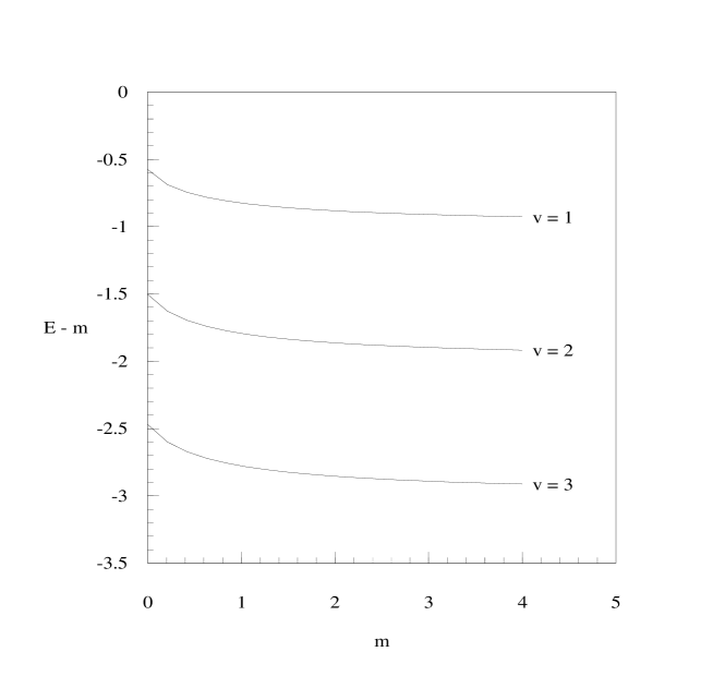
Figure 1: Plots of exact semirelativistic energies $E(m)-m$ for the nonlocal exponential potential ${\mathcal{V}}(x,x^{\prime})=-ve^{-|x|-|x^{\prime}|}$ for three values of the coupling $v.$

3.2 A two-term exponential potential

We consider now the case

$${\mathcal{V}}(x,x^{\prime})=-v_{a}e^{-(|x|+|x^{\prime}|)/a}-v_{b}e^{-(|x|+|x^{\prime}|)/b},\quad v_{a},\ v_{b},\ a,\ b\ >0.$$

In particular, if we choose the explicit values $a=1,b=2,v_{a}=v_{b}=1,$ the secular equation (2.10) becomes

$$(1-J_{11})(1-J_{22})-J_{12}^{2}=0,$$

where the integrals are given by

$$J_{11}={4\over{\pi}}\int\limits_{0}^{\infty}{dk\over{(1+k^{2})^{2}(\sqrt{m^{2}+k^{2}}-E)}},$$

$$J_{22}={16\over{\pi}}\int\limits_{0}^{\infty}{dk\over{(1+4k^{2})^{2}(\sqrt{m^{2}+k^{2}}-E)}},$$

and

$$J_{12}={8\over{\pi}}\int\limits_{0}^{\infty}{dk\over{(1+k^{2})(1+4k^{2})(\sqrt{m^{2}+k^{2}}-E)}}.$$

Thus for $m=\{0,~{}0.5,~{}1\}$ we find respectively from (3.9) that $E=\{-1.14462,~{}-0.814543,~{}-0.36131\}.$ In Fig.(2) we exhibit a graph showing $E-m$ as a function of $m$ for this problem.

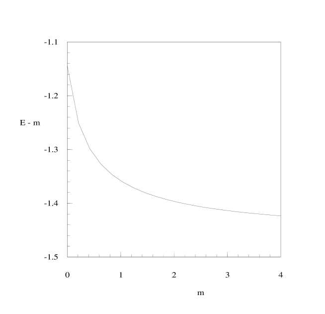
Figure 2: Plots of exact semirelativistic energies $E(m)-m$ for the nonlocal two-term exponential potential ${\mathcal{V}}(x,x^{\prime})=-e^{-(|x|+|x^{\prime}|)}-e^{-\frac{1}{2}(|x|+|x^{\prime}|)}.$

4 Problems in three dimensions

The Yamaguchi potential [4] has a potential kernel given by

$${\mathcal{V}}({\bf r},{\bf r^{\prime}})=-v\left(\frac{e^{-\beta r}}{r}\right)\left(\frac{e^{-\beta r^{\prime}}}{r^{\prime}}\right),\quad v,~{}\beta>0.$$

Because of the volume measure $r^{2}dr$ in three dimensions cancels the singularities in the Yukawa-type factors, this problem is very similar to the exponential potential in one dimension. The wave function and eigenvalue formula are found from (2.13) and (2.14) to be respectively

$$\tilde{\psi}(k)=\frac{c}{\left(k^{2}+\beta^{2}\right)\left(\sqrt{m^{2}+k^{2}}-E\right)}$$

and

$$\frac{1}{v}=8\int\limits_{0}^{\infty}\frac{k^{2}dk}{\left(k^{2}+\beta^{2}\right)^{2}\left(\sqrt{m^{2}+k^{2}}-E\right)}.$$

Thus the energy $E$ may be found from (4.3) as a function of the positive parameters $\{m,\beta,v\}.$

Similarly, for the Gauss potential we have the kernel

$${\mathcal{V}}({\bf r},{\bf r^{\prime}})=-ve^{-{\textstyle\frac{1}{2}}\beta(r^{2}+r^{\prime 2})}\quad v,~{}\beta>0.$$

The corresponding wave function and eigenvalue formula in this case are given by

$$\tilde{\psi}(k)=\frac{ce^{-{\textstyle\frac{1}{2}}k^{2}/\beta}}{\sqrt{m^{2}+k^{2}}-E}$$

and

$$\frac{1}{v}=\frac{4\pi}{\beta^{3}}\int\limits_{0}^{\infty}\frac{e^{-k^{2}/\beta}k^{2}dk}{\sqrt{m^{2}+k^{2}}-E}.$$

5 The semirelativistic $N$-boson problem

In this section we consider a system of $N$ identical bosons interacting pairwise in three spatial dimensions. The Hamiltonian for the system may be written

$$H=\sum_{i=1}^{N}(m^{2}+p_{i}^{2})^{{\textstyle\frac{1}{2}}}+\sum_{j>i=1}^{N}\hat{V}_{ij},$$

where, for a single particle, the action of the Gauss potential is given by

$$\hat{V}\psi({\bf r})=-v\int e^{-\frac{\beta}{2}(r^{2}+r^{\prime 2})}\psi({\bf r^{\prime}})d^{3}{\bf r^{\prime}},\quad v>0.$$

We shall consider two distinct approaches. First we obtain a lower bound to the lowest $N$-body energy $E$ with the aid of a scaled one-body problem and secondly we find an upper bound with the aid of an $N$-body Gaussian trial wave function.

5.1 The lower bound

If we suppose that $\Psi$ is the exact (unknown) $N$-boson wave function, then boson symmetry implies that $E=(\Psi,H\Psi)=(\Psi,h\Psi),$ where $h$ is a two-body Hamiltonian given by

$$h=\frac{N}{2}\left[(m^{2}+{\bf p}_{1}^{2})^{{\textstyle\frac{1}{2}}}+(m^{2}+{\bf p}_{2}^{2})^{{\textstyle\frac{1}{2}}}+(N-1)\hat{V}_{12}\right]$$

If new coordinates for the two-body problem are ${\bf r}={\bf r}_{1}-{\bf r}_{2}$ and $\rho={\bf r}_{1}+{\bf r}_{2},$ then the individual momenta are given by $\pi\pm{\bf p},$ and, by using the lemma of Ref. [11] to ‘remove’ the operator $\pi$ from within expectation values, the two-body operator $h$ may be replaced by ${\mathcal{H}},$ where

$${\mathcal{H}}=N\left[(m^{2}+p^{2})^{{\textstyle\frac{1}{2}}}+{\textstyle\frac{1}{2}}(N-1)\hat{V}\right],$$

Thus we conclude that

$$E=(\Psi,H\Psi)=(\Psi,{\mathcal{H}}\Psi)\geq{\mathcal{E}}=E_{L},$$

where ${\mathcal{E}}$ is the bottom of the spectrum of the one-body operator ${\mathcal{H}}.$ By comparing (5.4) with (4.6) we see that

$$\frac{1}{(N-1)v}=\frac{2\pi}{\beta^{3}}\int\limits_{0}^{\infty}\frac{e^{-k^{2}/\beta}k^{2}dk}{\sqrt{m^{2}+k^{2}}-E_{L}/N}.$$

Thus, for each choice of the parameters $m$ and $\beta$, (5.5a) implies that $E_{L}/N$ is a function of $v(N-1).$ In the special case $m=\beta=1,$ we write this function as $f_{L}$ so that we have

$$E_{L}/N=f_{L}(v(N-1)).$$

We note the special critical coupling $u_{c}$ defined by $f(u_{c})=0$ is given by $v(N-1)|_{c}=0.527485.$

5.2 The upper bound

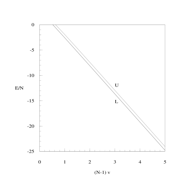
Figure 3: Upper and lower bounds for $E/N$ against $(N-1)v$ for $N$ identical bosons interacting via the Gauss pair potential ${\mathcal{V}}(r,r^{\prime})=-e^{-\frac{\beta}{2}(r^{2}+r^{\prime 2})}$ . The lower curve (L) is for $N=2$ and the upper curve (U) is for $N=\infty;$ the curves for $2<N<\infty$ lie between these two.

For a variational upper bound we adopt explicit relative coordinates. Jacobi coordinates may be defined with the aid of an orthogonal matrix $B$ relating the column vectors of the new $[\rho_{i}]$ and old $[{\bf r}_{i}]$ coordinates given by $[\rho_{i}]=B[{\bf r}_{i}].$ The first row of $B$ defines a center-of-mass variable $\rho_{1}$ with every entry $1/\sqrt{N},$ the second row defines a pair distance $\rho_{2}=({\bf r}_{1}-{\bf r}_{2})/\sqrt{2},$ and the $k\!$th row, $k\geq 2,$ has the first $k-1$ entries $B_{ki}=1/\sqrt{k(k-1)},$ the $k\!$th entry $B_{kk}=-\sqrt{(k-1)/k},$ and the remaining entries zero. We define the corresponding momentum variables by $[\pi_{i}]=(B^{-1})^{\rm t}[{\bf p}_{i}]=B[{\bf p}_{i}].$ The trial wave function we use is given by

$$\Phi(\rho_{2},\rho_{3},\dots,\rho_{N})=Ce^{-{{\alpha}\over{2}}\sum_{i=2}^{N}\rho_{i}^{2}}=C\prod\limits_{i=2}^{N}\phi(\rho_{i})$$

where $\alpha>0$ and $C$ is a normalization constant. This function is symmetric in the individual position coordinates $\{{\bf r}_{i}\}_{i=1}^{N}$ and also in the $N-1$ relative coordinates $\{\rho_{i}\}_{i=2}^{N};$ meanwhile it has the unique factoring property shown. These facts enable us [11] to express the expectation of the full Hamiltonian $H$ in the form

$$E\leq(\Psi,H\Psi)=N(\phi,\ ((m^{2}+2\lambda p^{2})^{{\textstyle\frac{1}{2}}}+(N-1)\hat{V})\phi),$$

where $\lambda=(N-1)/N,$ the potential operator $\hat{V}$ has the Gauss kernel (4.4), and $\alpha$ is to be used as a variational parameter. We therefore obtain the following expression for the upper bound $E_{U}$ in the special case $m=\beta=1$

$$\frac{E}{N}\leq\frac{E_{U}}{N}=\left(\frac{2}{\pi}\right)^{{\textstyle\frac{1}{2}}}\min_{s>0}\left[\frac{g(s^{2})}{s}-8v\pi^{2}\frac{(2\lambda s^{2})^{\frac{3}{2}}}{(1+4\lambda s^{2})^{3}}\right],$$

where the monotone function $g$ is given by

$$g(x)=\int_{-\infty}^{\infty}e^{-t^{2}}\left[2x+t^{2}\right]^{{\textstyle\frac{1}{2}}}t^{2}dt=xe^{x}K_{1}(x).$$

In this last expression, $K_{\nu}(x)$ is a modified Bessel function of the second kind [12]. The result of the minimization in (5.8a) yields $E_{U}/N$ as a function $f_{U}$ of $(N-1)v$ and $\lambda,$ where ${\textstyle\frac{1}{2}}\leq\lambda\leq 1.$ We have

$$E_{U}/N=f_{U}(v(N-1),\lambda).$$

Thus we obtain a different upper-bound curve for each $\lambda=(N-1)/N.$ These curves do not intersect. In Fig.(3) we exhibit the lower curve $f_{L}(v(N-1)),$ valid for all $N$, the upper curve $f_{U}(v(N-1),{\textstyle\frac{1}{2}}),$ for $N=2,$ and the upper curve $f_{U}(v(N-1),1),$ for $N=\infty.$ For the case $N=2$ the general lower (all $N\geq 2$) and particular upper bounds ($N=2$) are so close that they are indistinguishable on the graph: we have, for example, $f_{L}(1)=-2.56844$ and $f_{U}(1,{\textstyle\frac{1}{2}})=-2.5651$ approximately. Thus the scale-optimized Gaussian trial function is very effective for all $N,$ and particularly so for $N=2.$ The apparent straightness of the energy curves can perhaps be understood by reasoning such as the following: for the lower bound (5.5a), the Gaussian in the integrand decays rapidly to zero, thus the mean-value theorem tells us, for a given $v$, that $(N-1)v=A-B(E_{L}/N);$ it remains, of course, to explain why $A$ and $B$ vary very slowly with $v.$However, with exact analytical results available (for both bounds), we do not have to look for more analytical approximations.

6 Conclusion

We have shown that exact solutions can be found to semirelativistic eigenvalue problems when the potential has a kernel that is a sum of separable terms. This immediately extends, of course, to the wider class of $L^{2}$ kernels. It may be possible to use such exact solutions to approximate the spectra generated by local potentials. The non-relativistic many-body problem with non-local potentials has already been studied [9] and the present paper extends these results to the corresponding semirelativistic case. We have obtained tight bounds for the local semirelativistic $N$-body problem with local harmonic-oscillator potentials $V(r)=vr^{2}$, and somewhat weaker bounds for convex transformations $g(r^{2})$ of the oscillator [10]. The work reported in the present paper will no doubt help us to extend these semirelativistic many-body results to wider classes of potentials. It is very helpful when the lower bound itself, which is derived from a scaled one-body problem, can be found exactly. Improvements in the general lower bound await a treatment based on Jacobi relative coordinates; this has already been achieved in particular for the oscillator; the search for an improved general lower bound can now benefit from a non-oscillator test model for which there is also an accurate variational upper bound.

References

- [1] E. E. Salpeter and H. A. Bethe, Phys. Rev. 84, 1232 (1951).
- [2] E. E. Salpeter, Phys. Rev. 87, 328 (1952).
- [3] E. H. Lieb and M. Loss, Analysis (American Mathematical Society, New York, 1996). The definition of the Salpeter kinetic-energy operator is given on p. 168.
- [4] Y. Yamaguchi, Phys. Rev. 95, 1628 (1954).
- [5] T. Mukherjee, M. M. Mukhergee, A. Kundu, and B. Dutta-Roy, J. Phys. A 28, 2353 (1995)
- [6] P. Lévay, J. Phys. A30, 7243 (1997)
- [7] A. B. Balantekin, J. F. Beacom, and M. A. Cândido Ribeiro, J. Phys. G 24, 2087 (1998)
- [8] O. Kidun, N. Fominykh, and J. Berekadar, J. Phys. A 35, 9413 (2002)
- [9] R. L. Hall, Z. für Phys. A 291, 255 (1979)
- [10] R. L. Hall, W. Lucha, and F. F. Schöberl, J. Math. Phys. 45 3086 (2004)
- [11] R. L. Hall, W. Lucha, and F. F. Schöberl, J. Math. Phys. 43, 1237 (2002); J. Math. Phys. 44, 2724 (2003).
- [12] M. Abramowitz and I. A. Stegun (eds.) Handbook of Mathematical Functions with Formulas, Graphs, and Mathematical Tables (Dover, New York, 1972).