Singularities on charged viscous droplets

Abstract

We study the evolution of charged droplets of a conducting viscous liquid. The flow is driven by electrostatic repulsion and capillarity. These droplets are known to be linearly unstable when the electric charge is above the Rayleigh critical value. Here we investigate the nonlinear evolution that develops after the linear regime. Using a boundary elements method, we find that a perturbed sphere with critical charge evolves into a fusiform shape with conical tips at time $t_{0}$, and that the velocity at the tips blows up as $(t_{0}-t)^{\alpha}$, with $\alpha$ close to $-1/2$. In the neighborhood of the singularity, the shape of the surface is self-similar, and the asymptotic angle of the tips is smaller than the opening angle in Taylor cones.

One of the leading problems in fluid dynamics is the formation of singularities on charged masses of fluid. These problems are relevant in a variety of physical and technological situations, such as the breakup of water droplets in thunderstorms, electrospraying and electropainting.

Here we provide evidence of the formation of finite time singularities on electrically charged droplets of a conducting viscous fluid immersed in a dielectric viscous fluid of infinite extent. These singularities appear as the finite-time formation of conical tips at the surface and the blow-up of the velocity field at that point.

The interest in the shape of electrified drops dates back to Lord Rayleigh [2], who showed that if the electric charge is larger than some critical value, then a spherical drop becomes unstable. For a drop with total charge $Q$, surface tension coefficient $\gamma$ and radius $R$ suspended in a medium of dielectric constant $\varepsilon_{0}$, this critical value is $Q_{c}=\sqrt{32\gamma\pi^{2}\varepsilon_{0}R^{3}}$. After the drop becomes unstable, it desintegrates into droplets of smaller size. However, in recent experiments (see [3]) it has been noticed that previous to drop disintegration, the drop evolves into a prolate spheroid which, after a finite time, develops conical tips from which thin jets emerge.

This emission has been previously observed from a meniscus by Taylor, and is the basis of cone-jet electrospraying, a technique to produce microdroplets in a controlled fashion. A related technique, electrospray ionization, has revolutionized mass spectroscopy of large molecules. Applications to micro/nano encapsulation have also been developed recently (cf. [4]), and also the development of micro thrusters for the propulsion of spacecraft using liquid jets [7].

Here, by means of a numerical calculation and asymptotic analysis, we find that droplets with Rayleigh’s critical charge evolve into fusiform shapes with cones at the tips. On the course of this evolution, both the curvature and the fluid velocity at the tips diverge as $(t_{0}-t)^{\alpha}$, where $t_{0}$ is the time at which the cones are formed and the exponent $\alpha$ is approximately $-1/2$. Moreover, the numerical experiments indicate that the local shape of the surface is self-similar. The semiangle of the conical tips depends on the contrast of viscosities between the outer and inner fluids, and is close to $25$ degrees.

The existence of cones at the surface of a charged fluid is known since the work of Taylor (cf. [1]), who computed static solutions at the surface of a charged conducting fluid under the influence of an electric field. These solutions are nowadays known as Taylor cones, and possess a typical opening semiangle of $49.3^{o}$. The cones that we study here are different from the Taylor cones since they are dynamic. We shall refer to them as dynamic Taylor cones. A conclusion of our study is that static Taylor cones are not the generic singular structures developing during the evolution of the surface of a charged drop. In future publications we will analyze how the dynamic solutions can be continued after the formation of cones and determine whether jets or a string of droplets are produced.

We assume that the drop occupies a region $\Omega(t)$. Since the drop is a conductor, all the electric charge will be located at the boundary $\partial\Omega$, and since the surrounding medium is a dielectric, the total charge $Q$ remains constant. The electric field $\mathbf{E}$ outside the drop is given by $\mathbf{E}=-\nabla V$ where $\Delta V=0\;\;\mbox{ in }R^{3}\backslash\Omega,$ $V=C\;\;\mbox{ on }\partial\Omega$ and $V$ decays at infinity. At the surface of a conductor, the surface charge density $\sigma$ is given by the normal derivative of the potential, $\sigma=-\varepsilon_{0}\frac{\partial V}{\partial n}$, so that the repulsive electrostatic force per unit area is

$$\mathbf{F_{e}}=\frac{\mathbf{E}\sigma}{2}=\frac{\varepsilon_{0}}{2}\left(\frac{\partial V}{\partial n}\right)^{2}\mathbf{n}=\frac{\sigma^{2}}{2\varepsilon_{0}}\mathbf{n}$$ (1)

where $\mathbf{n}$ is the outward normal to the surface.

The fluid velocity $\mathbf{u}$ and the fluid pressure $p$ inside the drop satisfy the Stokes equations

$$-\nabla p+\mu_{1}\Delta\mathbf{u}=0\;\;\mbox{in }\Omega(t),$$ (2)

$$\nabla\cdot\mathbf{u}=0\;\;\mbox{in }\Omega(t)$$ (3)

where $\mu_{1}$ is the viscosity of the liquid inside the drop. Equations similar to (2) and (3) must be satisfied by the velocity and the pressure outside of the drop, $\mathbf{R}^{3}\backslash\Omega(t)$, with $\mu_{1}$ replaced by $\mu_{2}$, the viscosity of the surrounding liquid.

The boundary condition for the stress is

$$(T^{(2)}-T^{(1)})\mathbf{n}=\left(\gamma\kappa-\frac{\sigma^{2}}{2\varepsilon_{0}}\right)\mathbf{n}\;\;\mbox{ on }\partial\Omega(t),$$ (4)

where $\kappa$ is the mean curvature of the surface and $T^{(k)}$ is the stress tensor inside ($k=1$) or outside ($k=2$) the drop, given by

$$T_{ij}^{(k)}=-p\delta_{ij}+\mu_{k}\left(\frac{\partial u_{i}}{\partial x_{j}}+\frac{\partial u_{j}}{\partial x_{i}}\right)\;\mbox{, }k=1,2\;.$$ (5)

Equation (4) expresses the balance between viscous stress, capillary forces and electrostatic repulsion. The kinematic condition is

$$v_{N}=\mathbf{u}\cdot\mathbf{n}\;\;\mbox{ on }\partial\Omega(t)$$ (6)

where $v_{N}$ is the normal velocity of the free boundary $\partial\Omega(t)$.

Our numerical method to compute the evolution of the drop is based on the boundary integral method for the Stokes system (see [5], [6] for a comprehensive explanation). In this method, the equation for the velocity at $\partial\Omega(t)$ is written in integral form as

$$u_{j}(\mathbf{r}_{0}) = -\frac{1}{4\pi}\frac{1}{\mu_{1}+\mu_{2}}\int_{\partial\Omega(t)}f_{i}(\mathbf{r})G_{ij}(\mathbf{r},\mathbf{r}_{0})dS(\mathbf{r})$$

$$-\frac{1}{4\pi}\frac{\mu_{2}-\mu_{1}}{\mu_{2}+\mu_{1}}\int_{\partial\Omega(t)}u_{i}(\mathbf{r})T_{ijk}(\mathbf{r},\mathbf{r}_{0})n_{k}(\mathbf{r})dS(\mathbf{r})\;.$$

where

$$G_{ij}(\mathbf{r},\mathbf{r}_{0}) = \frac{\delta_{ij}}{\left|\mathbf{r}-\mathbf{r}_{0}\right|}+\frac{(r_{i}-r_{0,i})(r_{j}-r_{0,j})}{\left|\mathbf{r}-\mathbf{r}_{0}\right|^{3}}$$ (8)

$$T_{ijk}(\mathbf{r},\mathbf{r}_{0}) = -6\frac{(r_{i}-r_{0,i})(r_{j}-r_{0,j})(r_{k}-r_{0,k})}{\left|\mathbf{r}-\mathbf{r}_{0}\right|^{5}}$$ (9)

$$f_{i}(\mathbf{r}) = \left[\gamma(\mathbf{r})-\frac{\varepsilon_{0}}{2}\left(\frac{\partial V}{\partial n}\right)^{2}(\mathbf{r})\right]n_{i}(\mathbf{r}).$$ (10)

The equation for the charge density is

$$V(\mathbf{r}_{0})=\frac{1}{4\pi}\int_{\partial\Omega(t)}\frac{\sigma(\mathbf{r})}{|\mathbf{r-r_{0}}|}dS(\mathbf{r}).$$ (11)

This integral equation must be inverted numerically to obtain the charge density. $V(\mathbf{r}_{0})$ is a constant along the surface, and it is determined by the condition

$$Q=\int_{\partial\Omega(t)}\sigma(\mathbf{r})dS(\mathbf{r}).$$ (12)

Then we discretize the axisymmetric surface with $N$ conical rings and the velocity and the potential are approximated by constants within each ring. This leads to a system of linear equations that is solved using the LU decomposition. Our method increases its stability by applying a singularity removal procedure as explained in section 6.4 (formula 6.4.3) of [5]. As we are restricted to axisymmetric configurations, the surface integrals in (Singularities on charged viscous droplets) transform then into line integrals with kernels given in terms of elliptic functions (see section 2.4 in [5]). We validated the numerical scheme by comparing the numerical solutions with the linearized theory for viscous drops, that describes the evolution of small amplitude deformations.

As the initial condition, we start with a spherical droplet perturbed with a spherical harmonic $r(\theta)=R+\epsilon Y_{2}^{0}(\theta)$, where $r,\theta$ are the spherical coordinates with origin at the center of the drop. We found that the results are not sensitive on the value of $\epsilon$, as long as it is smaller than $0.1$. Here we will show the results for this value of $\epsilon$.

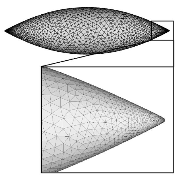
In figure 1 we show the drop profiles at several times approaching the singularity, that shows as conical tips at both ends of the drop.

Figure 1: Evolution of droplets with critical charge, with ratios of viscosities $\mu_{1}/\mu_{2}=100$ (top) and $1$ (bottom). Notice the tendency to develop conical tips.

The singularity occurs provided that the ratio of viscosities $\mu_{1}/\mu_{2}$ is large enough. Otherwise, the tips do not appear, and the drop tends to separate into smaller droplets. Our numerical computations show that the transition occurs between $\mu_{1}/\mu_{2}=0.1$ and $0.2$.

In figure 2 we show a close up in the region around the singularity. We translate the $(r,z)$ coordinates laterally by an amount $z_{f}=z(0,t)$ and then multiply them by the curvature at the tip of the drop $k_{f}$. The figure shows that the local shape near the tip is nearly invariant, and then by definition, the solution is self-similar.

Figure 2: Evolution of droplets with critical charge, with ratios of viscosities $\mu_{1}/\mu_{2}=100$ (top) and $1$ (bottom). We rescaled the free surfaces to make evident the self-similarity of the shapes. The curvatures at the tip are $146.7,92.1,77.5$ and $45.3$ for the figure on the top, and $1739,698,112$ and $65$ for the figure at the bottom.

In figure 3 we show plots of the velocity and charge density at the tip (the point of maximum curvature), as a function of time. This behaviour suggests a power-law or self-similar regime near the time of the singularity. We also show the potential $V$ at the surface to show that it does not diverge near the time of the formation of the tip. The Reynolds number, defined as $v_{f}/k_{f}$, remains bounded, which indicates that the hypothesis of the Stokes approximation are not violated near the singularity time $t_{0}$.

Figure 3: Maximum charge density and fluid velocity at the surface of droplets with critical charge, with ratios of viscosities $\mu_{1}/\mu_{2}=1$. The line on the top is a power law with exponent $-1/2$. The potential $V$ and the Reynolds number $Re$ are bounded during the evolution.

The angle of the conical tips depends weakly on the ratios of viscosities, as shown in figure 4, and as mentioned above, it is much smaller than the Taylor cone angle ($49.3^{o}$).

Figure 4: Semiangle of the conical tips, as a function of the ratio of viscosities $\mu_{1}/\mu_{2}$.

The numerical calculation does not allow us to explore much further into the asymptotic regime $t\rightarrow t_{0}$. However we can argue with a scaling argument that the similarity exponent is $1/2$. We can also show that near the singularity, capillarity forces are negligible while electric forces are dominant.

Let us place the origin of coordinates at a singularity point, where the surface will eventually develop the vertex, and describe the free surface with the following selfsimilar shape

$$z=(t_{0}-t)^{\alpha}f\left(\rho\right)\ ,\hskip 28.45274pt\rho=r(t_{0}-t)^{-\alpha}$$ (13)

where $t_{0}$ is the time of formation of the singularity and $\alpha>0$ is a similarity exponent, that will be deduced from scaling arguments.

The numerical evidence indicates (figure 3) that the electric potential $V$ at the surface is a continuous bounded function on the variable $t$, and $V$ has a non-zero limit as $t\rightarrow t_{0}$.Then if we assume a similarity solution for $V$ at the surface, it must have the form

$$V=\Phi\left(r(t_{0}-t)^{-\alpha}\right)$$ (14)

and then

$$\sigma=-\varepsilon_{0}\frac{\partial V}{\partial n}=(t_{0}-t)^{-\alpha}\Sigma\left(r(t_{0}-t)^{-\alpha}\right),$$ (15)

and in particular, the charge density at the tip of the drop is proportional to $1/(t_{0}-t)^{\alpha}$.

Since the mean curvature is given by

$$\kappa=\frac{1}{2}\left(\frac{1}{R_{1}}+\frac{1}{R_{2}}\right)\sim K(t_{0}-t)^{-\alpha}\;\mbox{ as }\;t\rightarrow t_{0},$$ (16)

where the $\sim$ symbol means “asymptotically proportional to”, and

$$\frac{\varepsilon_{0}}{2}\left(\frac{\partial V}{\partial n}\right)^{2}=\frac{\sigma^{2}}{2\varepsilon_{0}}\sim C^{\prime}(t_{0}-t)^{-2\alpha}\gg C(t_{0}-t)^{-\alpha},\mbox{ as }t\rightarrow t_{0}$$ (17)

we can conclude that capillary forces are negligible in comparison with the electrostatic forces near the singularity.

Figure 5: Evolution of a three dimensional drop: the singularity also develops in a 3D flow and the surface develops the same conical tips.

Figure 6: Evolution of a non-symmetric drop, and the formation of conical tips.

Then, the balance of stresses at the surface yields $\left|\mathbf{n}(T^{(2)}-T^{(1)})\mathbf{n}\right|\sim C^{\prime}(t_{0}-t)^{-2\alpha}$, from which we deduce typical pressure and velocity gradients $p,u_{i,j}\sim O\left((t_{0}-t)^{-2\alpha}\right)$, and hence velocities

$$u_{i}\sim O\left((t_{0}-t)^{-\alpha}\right).$$ (18)

By Eq. (13), $\mathbf{r}_{t}\sim O\left((t_{0}-t)^{\alpha-1}\right)$, which together with the kinematic condition at the surface $\mathbf{r}_{t}=\mathbf{u}$ and (18) imply $\alpha-1=-\alpha$ and therefore $\alpha=\frac{1}{2}.$ Hence the solutions of the Stokes system near the singularity are expected to have the form $p=(t_{0}-t)^{-1}P\left(\xi,\rho\right)$ and $\mathbf{u}=(t_{0}-t)^{-\frac{1}{2}}\mathbf{U}\left(\xi,\rho\right)$, with $\rho=r(t_{0}-t)^{-\frac{1}{2}}$ and $\xi=z(t_{0}-t)^{-\frac{1}{2}}$.

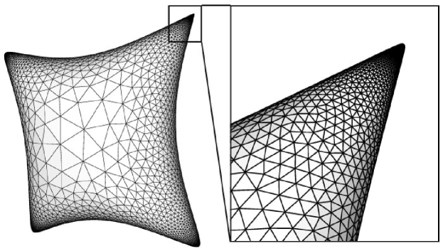
By relaxing the assumption of circular symmetry, conical tips still are developed. In order to show this, we implemented another numerical simulation based on the boundary elements method with adaptive triangulated surfaces to handle general three dimensional situations. Then we introduce a sphere perturbed with the mode $Y_{2}^{0}$ as an initial condition with critical charge, but, because we are approximating the shape of the surface with triangles, the numerical approximation is not axially symmetric. The result is in figure 5: the global shape is still axially symmetrical at the time of singularity formation. This is strong evidence of the stability of the self-similar solutions. On the other hand, the formation of singularities does not appear to be restricted to circularly symmetric flows: we found that they can also appear on asymmetric configurations. In figure 6 we show the evolution of an initial surface composed by an oblate ellipsoid with an asymmetric perturbation, with a supercritical charge $Q=1.2Q_{c}$. It can be clearly seen the tendency to develop a conical tip after the evolution. Moreover, the local shape of the tip is circularly symmetric, and the angle of the tip is approximately $25^{o}$, of the same order of magnitude as the angle on the symmetric shapes. This is a further indication that the singularity angle is fairly insensitive to the initial condition, and that it is smaller than Taylor’s value.

References

- [1] G. I. Taylor, Disintegration of water drops in an electric field, Proc. Roy. Soc. London A 280 (1964), 383-397.
- [2] Lord Rayleigh, On the equilibrium of liquid conducting masses charged with electricity, Phil. Mag. 14 (1882), 184-186.
- [3] D. Duft, T. Achtzehn, R. Müller, B. A. Huber and T. Leisner, Rayleigh jets from levitated microdroplets, Nature, vol. 421, 9 January 2003, pg. 128.
- [4] I. G. Loscertales, A. Barrero, I. Guerrero, R. Cortijo, M. Marquez, A. M. Gañan-Calvo, Micro/Nano Encapsutation Via Electrified Coaxial Liquid Jets, Science, Vol. 295, 5560 (2002), 1695-1698.
- [5] C. Pozrikidis, Boundary integral methods for linearized viscous flow, Cambridge texts in Applied Mathematics, Cambridge University Press, 1992.
- [6] J. M. Rallison, A. Acrivos, A numerical study of the deformation and burst of a viscous drop in an external flow, J. Fluid Mech. 89 (1978), 191-200.
- [7] M. Gamero-Castaño, V. Hruby, Electrospray as a source of nanoparticles for efficient colloid thrusters, J. Prop. Power 17 (2001), 977-987.