Abstract

The method of efficient description of long-term behavior of solutions of the non-linear first order ODE $\dot{\phi}+\sin\phi=f$ for arbitrary periodic $f$ is discussed. The criterion enabling one to separate and identify the qualitatively different solutions is established. The applications of the method to the modeling of dynamics of overdamped Josephson junctions in superconductors are outlined.

Preliminaries

A simple model of a Josephson junction [4] proposed by Stewart and McCumber [2, 3] is based, from the mathematical point of view, on the non-linear second order ODE

$$\beta\ddot{\phi}+\dot{\phi}+\sin\phi=f.$$ (1)

Here $\phi=\phi(t)$ is the unknown function (called phase) representing the difference of phases of the so called order parameter which plays the role of the macroscopic wave function describing the states of two weakly coupled superconducting electrodes constituting Josephson junction. The connection of the phase with observable quantities is established by the Josephson equation [1] which connects the voltage across the junction with the time derivative of $\phi$:

$$V={\Phi_{0}\over 2\pi}{d\phi\over d\tau}\propto\dot{\phi}\equiv{d\phi\over dt}.$$ (2)

Here the physical constant $\Phi_{0}=h(2e)^{-1}$ ($h$ is the Plank constant, $e$ is the electron charge) is called the (magnetic) flux quantum, the parameter $t$ used in Eq. (1) is the rescaled dimensionless time $t=\omega_{c}\tau$, where $\tau$ is the ‘genuine’ (dimensional) time, the constant $\omega_{c}$ called characteristic frequency is connected with junction properties. It can be defined by the equation $\omega_{c}=2\pi\Phi_{0}^{-1}R_{N}I_{c}$, where $R_{N},I_{c}$ are the junction characteristics, namely, $R_{N}$ is its resistance in the normal state, $I_{c}$ is called critical current (it estimates the maximal current which can flow through the junction without application of external voltage). The positive constant $\beta$ is connected with the junction capacitance, the less the latter, the less the former. The function $f=f(t)$ represents the current (normalized to $I_{c}$ and named bias) circulating in the junction circuit and supplied by an external source. It is assumed to be specified in advance.

Here we consider the case of a periodic bias of the known period $T$ and arbitrary profile. Thus $f$ is assumed to satisfy the condition

$$f(t)=f(t+T).$$ (3)

Usually $f$ is a continuous (or smooth) function but a finite number of finite jumps on the period interval is also allowed.

It is worth noting that there is a common practice in the physical literature to divide the periodic bias function $f$ into some constant constituent (‘direct current’, DC) $\iota_{\mbox{\scriptsize dc}}$ and the residual one $\iota_{\mbox{\scriptsize ac}}$ (alternating, high frequency, rf current, AC):

$$f=\iota_{\mbox{\scriptsize dc}}+\iota_{\mbox{\scriptsize ac}}.$$ (4)

Following this convention, we assume for definiteness that the average value of $f$ is assigned to $\iota_{\mbox{\scriptsize dc}}$. Accordingly, by definition, the average value of the residual $\iota_{\mbox{\scriptsize ac}}$ vanishes.

The important property of a Josephson junction, which is perfectly captured by the Stewart-McCumber model in spite of its comparative homeliness, is the phase-locking effect. Qualitatively, the phase-locking may be regarded as the relaxation in the course of the phase evolution of the ‘loose constituent’ of the phase function reflecting its initial state. Then the only surviving dynamical ‘process’ proves a steady one ‘dragged’ by the periodic bias and not depending of the past phase evolution. Said another way, once some lapse depending on the specific rate of relaxation of initial perturbations and the ‘magnitude’ of the latter elapses, the phase function profile proceeds with the reproducing itself, modulo a $2\pi$-aliquot contribution, on each subsequent time step of duration $T$. Obviously, such a situation would take place, in particular, if, regardless of the initial state the phase starts to evolve from, $\phi(t)$ converges for large $t$ to a periodic function of the period $T$. There are also other, non-periodic (but still fairly specific as we shall see below) forms of such an asymptotically ‘steady’ phase evolution. On the other hand, the phase-locking property is in no way a universal one to be automatically attributed to solutions of Eq. (1). Depending on the model parameters, the phase evolution may be completely different, revealing, in particular, no periodicity or any other apparent order [5].

Figure 1: Three subsequent segments (red, brown=$1\over 2$(red+green), green) of the single graph describing evolution of the phase function on the time interval $[0,3T]$ are placed over the common $t$-axes segment $[0,T]$ by means of appropriate ‘horizontal’ shifts ‘backwards in time’ (plot segmenting). The specific parameter value is $\iota_{\mbox{\scriptsize dc}}=0.8$ the values of other parameters are given in the main text. In order to visually resolve the neighbor graphs here (and in subsequent similar plots) all the curves, except for a starting one, are uniformly shifted in the ‘vertical’ direction by an additional amount of space which is uniformly incremented for each subsequent graph curve (here by 0.04 units). As one can see, the third (green) graph segment already coincides with the second one, essentially, yielding therefore the (approximate) specimen of the limiting phase evolution function which proves here periodic.

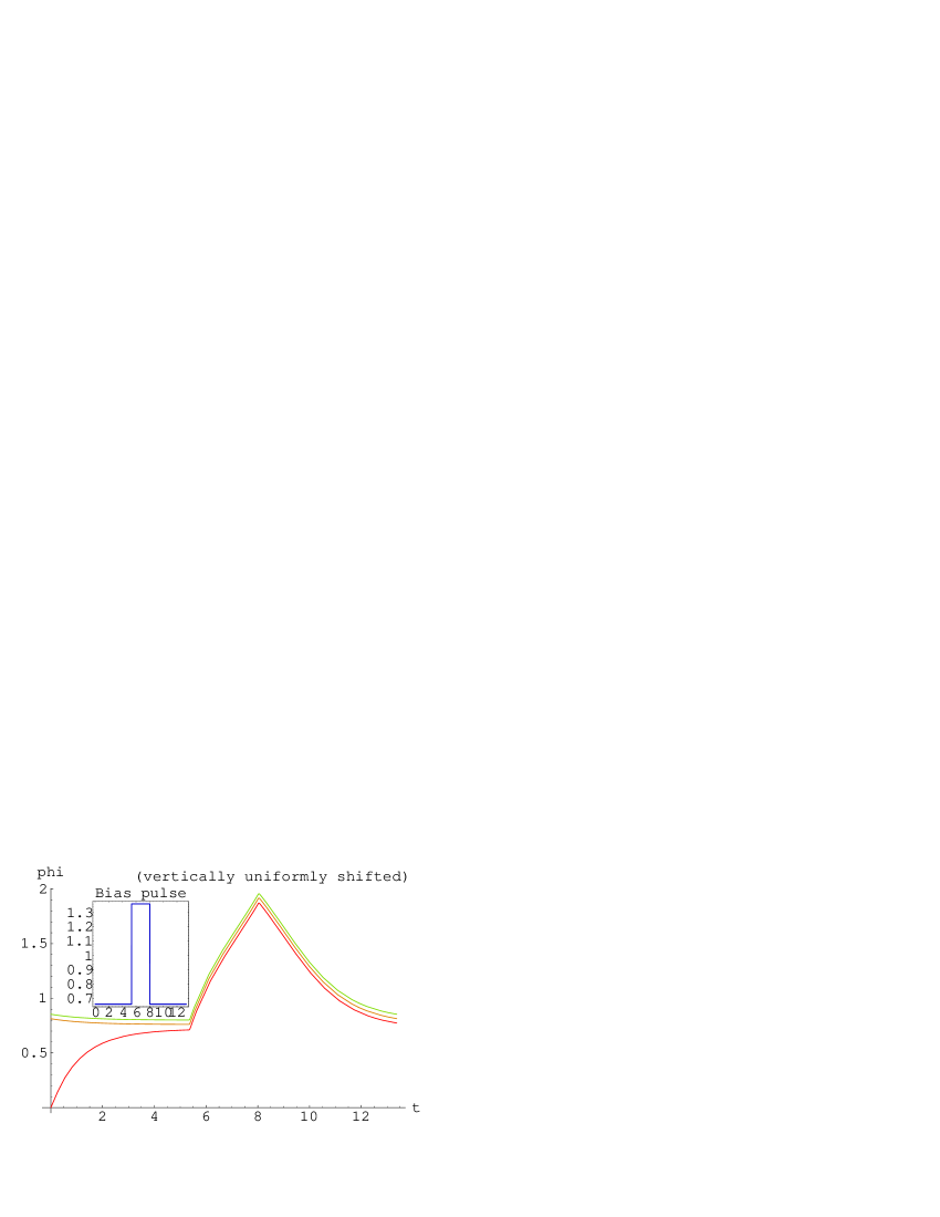
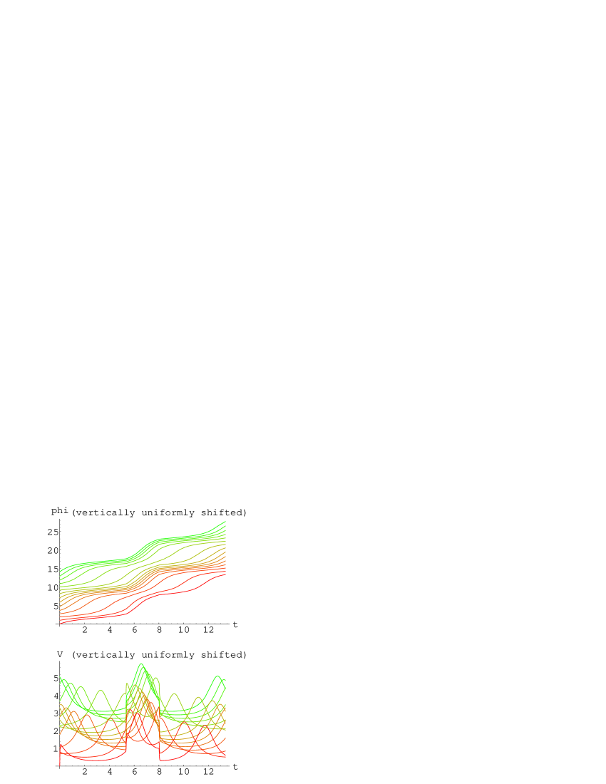
The plots shown in figure 1 illustrates the simplest case of the phase-locking in a numerical example. Here the result of a straightforward numerical integration of Eq. (1) is displayed. For the sake of definiteness, the bias function $f(t)$ is chosen to be the periodic rectangular pulse sequence, one of the pulses being shown in the inset. Its integral magnitude amounts to 1.5, the frequency is $2\pi/T=0.47$ ($T\simeq 13.3685$), $\beta=0.02$, the width of the pulse peak (here being rather a plateau symmetric with respect to the plot center) amounts to 20% of the total pulse period. The ‘constant bias constituent’ $\iota_{\mbox{\scriptsize dc}}$ (the average of $f$) equals $0.8$.

The phase evolution displayed in Fig. 1 starts with the null initial conditions $\phi(0)=0=\dot{\phi}(0)$ chosen for simplicity reasons. The figure displays the phase evolution during 3 sequential steps of variation of $t$, each of duration $T$. The graph of the first period phase evolution is of red color. The second period plot graph ($t\in[T,2T]$) is brown. To be placed over the same $t$-axes segment as the first graph, it is shifted to the left (‘backwards in time’) just by $T$. Similarly, the graph of the phase function over the third period time step ($t\in[2T,3T]$, the green curve) is shifted to the left by $2T$ that places it over the same $t$-axes segment $[0,T]$. As a result, all the three subsequent portions of the phase evolution graph are displayed over the common segment of the $t$-axes becoming more eligible for a visual collation and the monitoring of the $T$-scale periodicity.

In passing, it is worth emphasizing that due to periodicity of $f$ the functions resulted from the above ‘translations’ by means of the $t$-shifts aliquot $T$ retain to verify Eq. (1). Thus, applying such a trick, the ‘contiguous’ phase function representing the phase evolution over some time interval, perhaps semi-infinite, can be equally well represented by the sequence of phase functions (solutions of Eq. (1)) each defined on the finite interval $[0,T]$.

Besides, for the better clarity, some additional artificial uniformly incrementing vertical shifts are applied to separate graph segments in Fig. 1. The point is that we would like to recognize the limiting curve to which the sequence of the displayed ones converges, and the details of such a conversion, provided it takes place. Obviously, it is reasonable to add some uniformly incremented vertical space to the vertical positions of separate graph segments in order to visually distinguish the far mutually close curves which otherwise would be seen in the plot overlaid in a messy way. Specifically, in the case of Fig. 1, the vertical shifts amounting to additional 0.04 units per each subsequent graph segment are applied. This allows one to visually distinguish the second (brown) and the third (green) phase graph segments showing simultaneously that the corresponding functions are very close. In subsequent similar plots, the benefit of the trick will be ever more clear.

It turns out that under the conditions assumed, the phase function on the third time step (the third period) apparently coincides with the one on the second step and thus already represents, with accuracy characteristic for the plot resolution, the desirable limiting (asymptotic) phase time dependence. The $T$-scale convergence proves here extremely fast. It is also obvious that in view of the convergence of subsequent graph segments to the common limiting curve the values of $\phi$ on the left and right graph boundaries of its domain coincide, making evidence of the periodicity of the limiting solution of Eq. (1) we deal with.

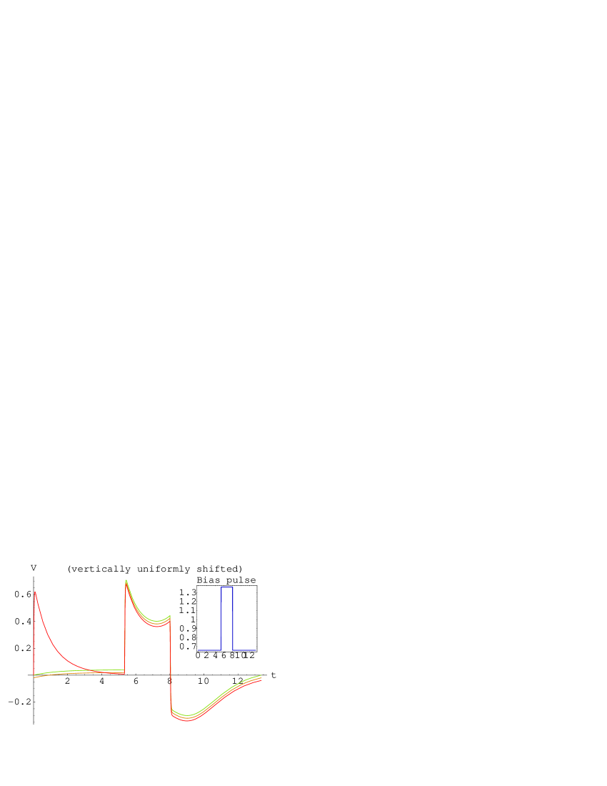
It is also of interest to consider the graphs of the corresponding voltage which coincides, up to the constant factor, with the derivatives of the functions displayed in Fig. 1. These are shown in Fig. 2, the vertical and horizontal shifts (the part of the plot segmenting trick) similar to ones in Fig. 1 being applied. The voltage functions also rapidly converge to a periodic limiting one.

Figure 2: The voltage across junction (in arbitrary units) is displayed for the phase functions shown in Fig. 1. In order to resolve the convergent series of graphs, the graphs except of the starting one are uniformly shifted in the ‘vertical’ direction, the trick similar to one applied in Fig. 1.

It has to be noted that the phase-locking does not necessarily claim for the asymptotic phase function $\phi(t)$ to be periodic. Indeed, keeping in mind the physical aspect of the problem, the actually registered voltage across Josephson junction is not momentary but is efficiently averaged over many bias periods $T$. For the sake of simplicity, let us consider the result of the voltage averaging over a single period (the shortest time interval making sense in the situation under consideration), treating the averaging as the plain integrating followed by the division by the length of the integration interval. Then in accordance with Eq. (2) the averaging started at the moment $t$ has to yield

$$\langle V\rangle_{\Delta t}=\Delta t^{-1}\int^{t+\Delta t}_{t}V(t^{\prime})dt^{\prime}\propto\Delta t^{-1}[\phi(t+\Delta t)-\phi(t)]$$ (5)

with $\Delta t=T$ (the proportionality relation means here the dropping out of a dimensional universal constant). Thus the (asymptotic) periodicity of $\phi$ means $\langle V\rangle_{T}=0$ implying that no average voltage across the junction is observed. However, instead of $f$ periodicity, one may also assume that the increment of $\phi$ across the time step of duration $T$ is independent on the moment ${t}$ when the averaging starts: $\phi({t}+T)-\phi({t})=\mbox{constant}$, asymptotically (for large but otherwise arbitrary $t$). This constant may not be arbitrary. The condition above is consistent with Eq. (1) if, asymptotically,

$$\phi({t}+T)-\phi({t})=2\pi k,$$ (6)

where $k$ is some integer, positive, negative, or zero. This number is named the phase-locking order. Evidently, the periodic phase function is the particular case corresponding to the zero order. Allowing arbitrary integer $k$, the average voltage proves quantized assuming, in principle, any of discrete uniformly distributed values.

Numerical integration of Eq. (1) allows one to easily confirm the feasibility of non-zero-order phase-locking phase functions. In particular, Fig. 3 displays the example of first order phase-locking. Here the only difference in the parameter setup with the zero order case (figures 1, 2) is the value of the parameter $\iota_{\mbox{\scriptsize dc}}$ now amounting to 1.1. The limiting phase function is here not periodic but its increments on the time steps of duration $T$ apparently tends to $2\pi$. On the other hand, subtracting the linearly growing contribution which insures this secular phase incrementing, a periodic function is leaved.

Figure 3: Example of the segmented phase function (top panel) and segmented voltage function (lower panel, arbitrary units) for the first order phase-locking state. The parameters of the model are the same as in figures 1, 2, except for $\iota_{\mbox{\scriptsize dc}}=1.1$. The color of subsequent phase function segments uniformly varies from red to green. The uniformly incremented shifts in the ‘vertical’ direction are applied including the first order phase-locking responsible contribution $-2\pi$ for the phase ($-2\pi$+0.2 units for the top panel and 0.2 units for the lower one per subsequent graph segment, respectively).

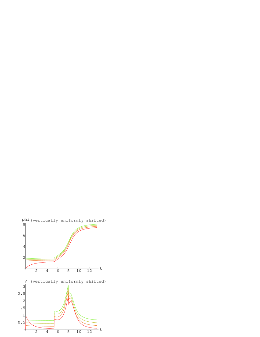
Similarly, the further increasing of $\iota_{\mbox{\scriptsize dc}}$ yields the second order phase-locking phase evolution. It is displayed in Fig. 4. Here $\iota_{\mbox{\scriptsize dc}}=1.4$, the other parameters being kept unchanged. Increasing $\iota_{\mbox{\scriptsize dc}}$, the larger order phase-locking phase functions can be produced as well.

Figure 4: Example of the phase-locking of the order two. The parameters of the model are the same as in figures 1-3, except for $\iota_{\mbox{\scriptsize dc}}=1.4$. The color of subsequent phase function segments (top panel) and voltage function segments (lower panel, arbitrary units) uniformly varies from red to green. The uniformly incremented shifts in the ‘vertical’ direction are similar to ones applied in Fig. 3 differing in the shift contribution for the phase connected with the non-zero order of the phase-locking which amounts here to $-4\pi$ instead of $-2\pi$ applied therein.

It is seen that in the cases of higher order phase-locking, the convergence of the sequence of segmented phase functions to the common limiting function is slower. Indeed, in the case of zero order phase-locking (Fig. 1, $\iota_{\mbox{\scriptsize dc}}=0.8$) the third iteration apparently coincided with the second one and yield, in fact, the limiting curve (the phase-locking order can be estimated from the asymptotic relation

$$k\simeq(2\pi)^{-1}[\phi(t+T)-\phi(t)]$$ (7)

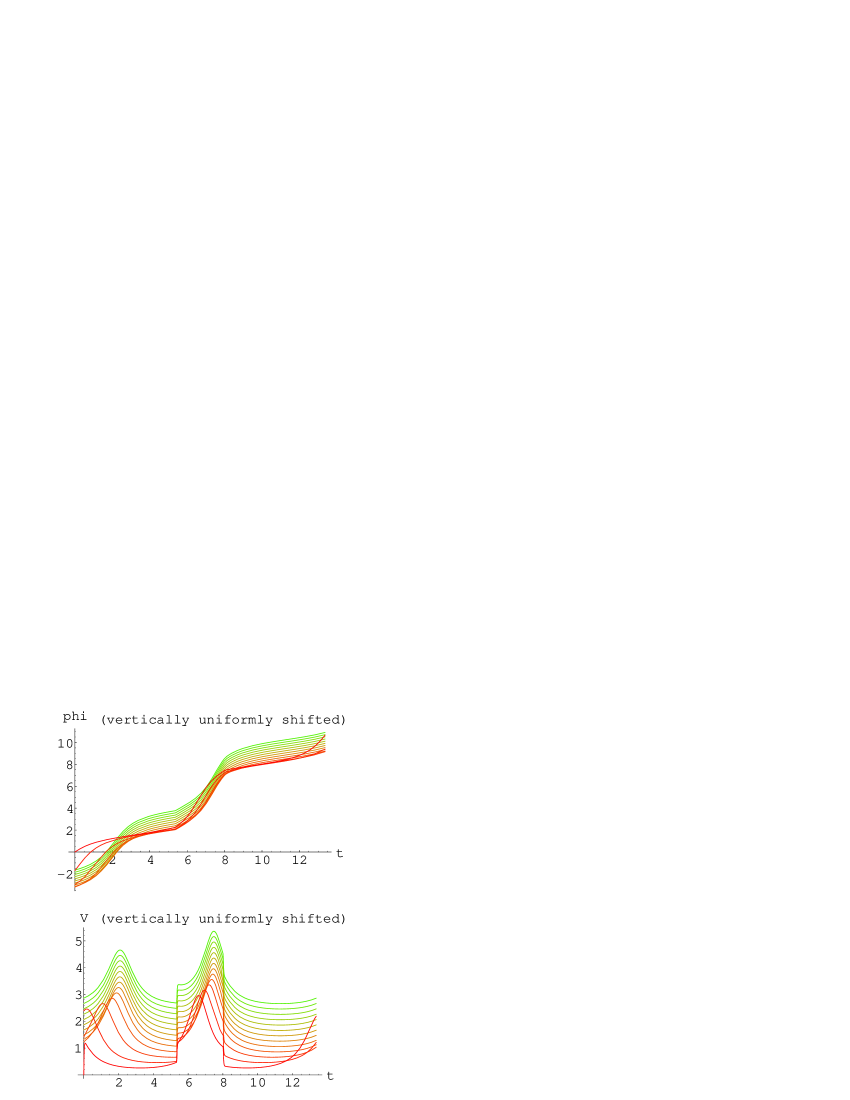
taking place for sufficiently large $t$ (formally, in the limit $t\rightarrow\infty$), provided the phase-locking is developed). In the case of the phase-locking of the first order observed in the case $\iota_{\mbox{\scriptsize dc}}=1.1$ the four $T$-lapses are needed for the reaching of a comparable closeness to the limit. For the phase-locking of the order two which takes place, in particular, if $\iota_{\mbox{\scriptsize dc}}=1.4$ the number of necessary iterations increases up to 15. And it suffices to set up $\iota_{\mbox{\scriptsize dc}}=1.45$ to lose the apparent convergence to any steady asymptotic state at all. The corresponding apparently non-convergent segmented phase and voltage function plots are shown in Fig. 5. These reveal no tendency to converge to any limiting curves demonstrating ‘irregular’ (or even apparently ‘chaotic’, as far as one concerns the variations on the scale $T$) behavior. The value of the expression (7), irregularly oscillating around 2, does not reveal apparent tending to any limit as well.

Figure 5: Example of asymptotically non-convergent (‘irregular’) evolution. The parameters of the model are the same as in figures 1-4, except of $\iota_{\mbox{\scriptsize dc}}=1.45$. The uniformly incremented shifts in the ‘vertical’ direction ($-4\pi+0.2$ units for the phase and 0.2 units for the voltage functions per subsequent graph segment, respectively) are applied.

It is worth mentioning that the convergence — or the divergence — of the sequence of phase functions describing a single long-term phase evolution is often difficult to reliably establish by means of straightforward numerical integrating of Eq. (1). Indeed, the slower such a sequence converges, the longer fragment of the phase evolution has to be analyzed. Accordingly, approaching the hypothetical boundary of the area in the space of the bias functions where the evolution of the phase leads to a steady state (phase-locking area in the parameter space), one inevitably encounters with insufficiency of the available computational resources. The very boundary, where the convergence reverses to the divergence, is not detectable in this way. Besides, in view of the obscurity of the corresponding time scale, the ‘strong’ phase divergence (more exactly, the absence of convergence to any asymptotic steady state) is even harder to detect through the apparent behavior of numerically generated phase function than the too slow convergence.

The formulation and substantiation of the method allowing one to efficiently distinguish the phase-locking property in the important particular case of ‘overdamped’ version of equation (1) is the main theme of the present discussion. The term ‘overdamped’ refers here the case

$$0\leq\beta\ll 1.$$ (8)

The parameter $\beta$ scales the (only) term involving the second order derivative of the phase function in Eq. (1). It might be supposed that under certain conditions including imposing of limitation on the second derivative values the relevant solutions of Eq. (1) may be approximated by the solutions of the equation

$$\dot{\phi}+\sin\phi=f$$ (9)

obtained from Eq. (1) by a mere discarding of the second order derivative term.

The numerical example illustrating the impact of the above ‘simplification’ is shown in Fig. 6, the discussion of the status of the corresponding approximation for ‘overdamped’ systems (in the case of sinusoidal bias $f$) can be found in [5].

In Fig. 6 the black curve represents the phase function computed in accordance with Eq. (9), the red one is the corresponding solution of the general RSJ-equation (1). The ‘red’ solution is shifted downward by 0.1 units in order to allow easier visual distinguishing of the close graphs on the common plot panel. The green curve represents the difference of the two phase functions above which is magnified by the factor of 10. The bias pulse is shown in the inset. Its form is similar to the ones used above, see Fig. 1, except for the bias ‘DC constituent’, $\iota_{\mbox{\scriptsize dc}}$, which is here chosen vanishing (i.e.  $\int^{T}_{0}f({t})d\,{t}=0$), and the integral magnitude of a single pulse which here and in all the numerical examples below amounts to 3.5.

Figure 6: The related solutions of Eqs. (1) (the red graph) and to (9) (the black one) for the same periodic rectangular pulse bias (shown in inset) displayed together with their difference magnified by the factor of 10 (the green graph) . The red plot is shifted downward by 0.1 units. The bias is the same as above except the parameter $\iota_{\mbox{\scriptsize dc}}$ which is now assumed to vanish and the pulse magnitude here equal to 3.5.

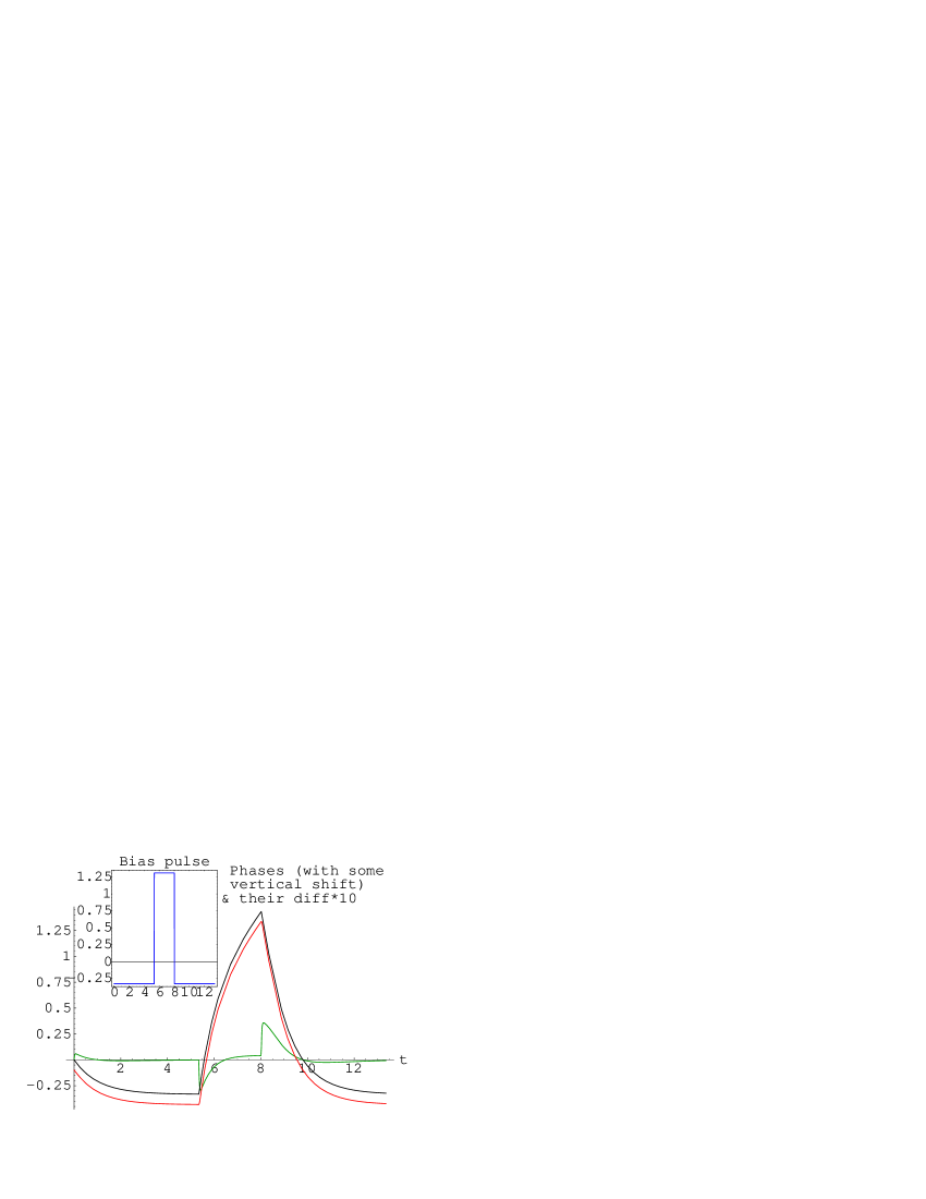
It is seen that under the conditions assumed the solutions of Eqs. (9) and (1) are very close, in total, both in shape and in magnitude, the deviations emerging at several moments of time ultimately relaxing. Specifically, the solution difference reveals the splashes originated in three points: at ${t}=0$, and on the front and back ‘shocks’ of the bias pulse. At right near them, the difference soon reaches a maximum and then quickly die. In total, the distinction of the corresponding solutions of Eqs. (1) and (9) may be considered fairly mild.

It is easy to see that the splash following the point ${t}=0$ arises due to the specific choice of the initial conditions for solution of Eq. (1) which read $\phi(0)=0=\dot{\phi}(0)$. Then Eq. (1) implies $\ddot{\phi}(0)=\beta^{-1}f(0)$ which, for $f(0)\not=0$, is a large quantity contrary to assumption required for approximating Eq. (1) by (9). In particular, it leads to the fast growth of the first derivative immediately after the start of the phase evolution. This effect is also observed in Fig. 2.

Apart of the apprehensible effect of non-equivalent initial conditions, the cause of the other discrepancy splashes is also quite understandable: they arise due to the discontinuities of the r.h.s. function $f$. Indeed, as a pulse front/back jump occurs, the discontinuity in $f$ converts to a finite jump in the derivative $\dot{\phi}$ in solution of Eq. (9) which, in turn, emerges the Dirac $\delta$ function-like irregularity in the second derivative $\ddot{\phi}$ which again violate the assumption of limitation of $\ddot{\phi}$ magnitude required for the approximating of solutions of (1) by solutions of Eq. (9).

Evidently, the cause of these peculiarities, leading to major distinctions of solutions of Eq. (1) and Eq. (9) shown in Fig. 6, originates in either the admitting somewhat inadequate initial conditions or in a too rough representation (by a discontinuous function) of the bias term. Since for a more physically realistic bias model no $\delta$-like irregularities of the phase derivative can arise, the agreement of the models based on Eqs. (1) and (9) would improve.

As compared to more deep Eq. (1) whose study is still possible by numerical methods alone, Eq. (9) proves more transparent and allows fairly deep analytical treatment. It seems also to be of interest in its own rights as the example of a non-linear problem of a deep physical relevance associated with a simple linear dynamical system. Eq. (9) possesses therefore a number of remarkable properties which are the subject of the discourse below.

The modeling of the phase dynamics

Master identity and its consequences

The approach to the problem of description of generic properties of solutions of Eq. (9) on the timescale exceeding the period $T$ including their asymptotic behavior can be based on the following observation:

Master identity 1

For any piecewise smooth continuous functions $\phi=\phi({t}),\phi_{0}=\phi_{0}({t})$, let us define the functions

$$P_{0} \equiv P_{0}({t})\equiv P_{0}[\phi_{0}]({t})=\int\cos\phi_{0}({t})\,d\,{t},$$ (10)

$$Q_{0} \equiv Q_{0}({t})\equiv Q_{0}[\phi_{0}]({t})=\int e^{-P_{0}({t})}\,\sin\phi_{0}({t})\,d\,{t},$$ (11)

and introduce the notations:

$$\zeta \equiv \zeta({t})=e^{\mathrm{i}\phi({t})},\enskip\zeta_{0}\equiv\zeta_{0}({t})=e^{\mathrm{i}\phi_{0}({t})},$$ (12)

$$C \equiv C[\phi,\phi_{0}]({t})=\left[-Q_{0}+\mathrm{i}e^{-P_{0}}{\zeta_{0}+\zeta\over\zeta_{0}-\zeta}\right]^{-1}.$$ (13)

Then the following identity takes place

$${1\over 2\mathrm{i}}(\zeta-\zeta_{0})^{2}e^{P_{0}}{dC^{-1}\over d\,{t}}\equiv\zeta_{0}D[\zeta]-\zeta D[\zeta_{0}]$$ (14)

with the differential operator $D[\cdot]$ is defined as follows

$$D[z]\equiv{dz\over d\,{t}}+{1\over 2}(z^{2}-1)-\mathrm{i}fz$$ (15)

for some function $f\equiv f({t})$ and arbitrary piecewise smooth $z\equiv z({t})$.

Its proof reduces to a straightforward computation applying definitions of the functions involved.$\square$

Remarks:

• For the sake of definiteness, the indefinite integrals in Eqs. (10,11) can be understood as $\int^{t}_{0}\dots d\,{t}$. Another choice of lower integration boundary would lead to a linear transformation of $C[\dots]^{-1}$: an overall constant factor is induced by the changing the lower boundary in the $P$-integral while a change of the lower boundary in $Q$-integral definition yields a constant summand.

• Solving Eq. (13) with respect to $\zeta$, one gets the equation

  $$\zeta=\zeta_{0}{1+C(Q_{0}-\mathrm{i}e^{-P_{0}})\over 1+C(Q_{0}+\mathrm{i}e^{-P_{0}})}.$$ (16)

  Assuming $P_{0},Q_{0}$ to be real, for complex valued $\zeta_{0},\zeta$ both of these variables can be unimodular, $|\zeta_{0}|=1=|\zeta|$ (and $\phi_{0},\phi$ real, see (12 )) if and only if $C$ is real.

The connection of the relationships inferred from the identity (14) with the equation (9) follows from the identity

$${d\zeta\over d\,{t}}+{1\over 2}(\zeta^{2}-1)-\mathrm{i}f\zeta\equiv\mathrm{i}\zeta(\dot{\phi}+\sin\phi-f),$$ (17)

provided $\zeta$ and $\phi$ are connected by Eq. (12). In conjunction with master identity, it immediately yields the following [7]

Proposition 1

Let $\phi_{0}({t})$ verify Eq. (9) whereas $P_{0}({t}),Q_{0}({t})$ be defined by Eqs. (10), (11). Then any solution $\phi({t})$ of Eq. (9) satisfies either the equation

$$e^{\mathrm{i}\phi({t})} = e^{\mathrm{i}\phi_{0}({t})}{1+C(Q_{0}-\mathrm{i}e^{-P_{0}})\over 1+C(Q_{0}+\mathrm{i}e^{-P_{0}})},$$ (18)

where $C$ is some real constant, or the equation

$$e^{\mathrm{i}\phi({t})} = e^{\mathrm{i}\phi_{0}({t})}{Q_{0}-\mathrm{i}e^{-P_{0}}\over Q_{0}+\mathrm{i}e^{-P_{0}}},$$ (19)

the latter being in fact the limiting form of the former as $C\rightarrow\infty$.

Remarks:

• When regarded as the relationship determining $\phi$, Eq. (18) or (19) specifies it not uniquely but modulo $2\pi$. On the other hand, this is the only arbitrariness involved in such a definition of $\phi(t)$.

• The initial, ‘ground’ solution $\phi_{0}$ is produced by the same equation (18) in the case $C=0$ when (18) converts to the identical transformation (modulo $2\pi$). That is why just $C$ rather than $C^{-1}$ which has a formally simpler representation in terms of $\phi$’s, see (13), is employed in (18).

• Given $\phi(0)$, the constant $C$ can be easily found. Indeed, it follows from Eq. (13) that, placing the left boundary of the integration interval at ${t}=0$, one has $P_{0}(0)=0=Q_{0}(0)$, that yields

  $$C=\mathrm{i}{e^{\mathrm{i}\phi(0)}-e^{\mathrm{i}\phi_{0}(0)}\over e^{\mathrm{i}\phi(0)}+e^{\mathrm{i}\phi_{0}(0)}}=-\tan\mbox{\scriptsize$1\over 2$}[\phi(0)-\phi_{0}(0)].$$ (20)

  Thus, given any particular solution of Eq. (9) and the integrals $P_{0}({t}),Q_{0}({t})$, defined from it by Eqs. (10), (11) and obeying the conditions $P_{0}(0)=0=Q_{0}(0)$, the solution of the Cauchy problem for Eq. (9) is explicitly represented (modulo $2\pi$) by Eqs. (18) and (20).

• In view of (20) one also gets

  $$C[\phi_{0},\phi]_{|t=0}=-C[\phi,\phi_{0}]_{|t=0}$$ (21)

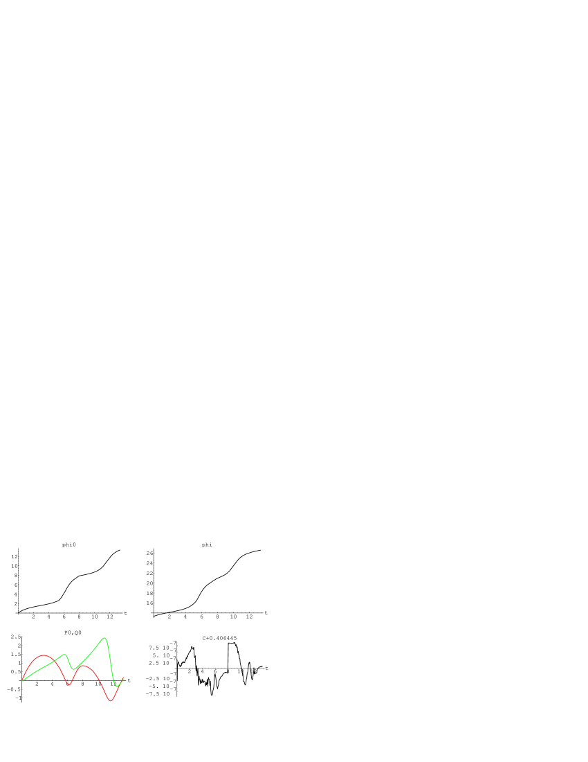
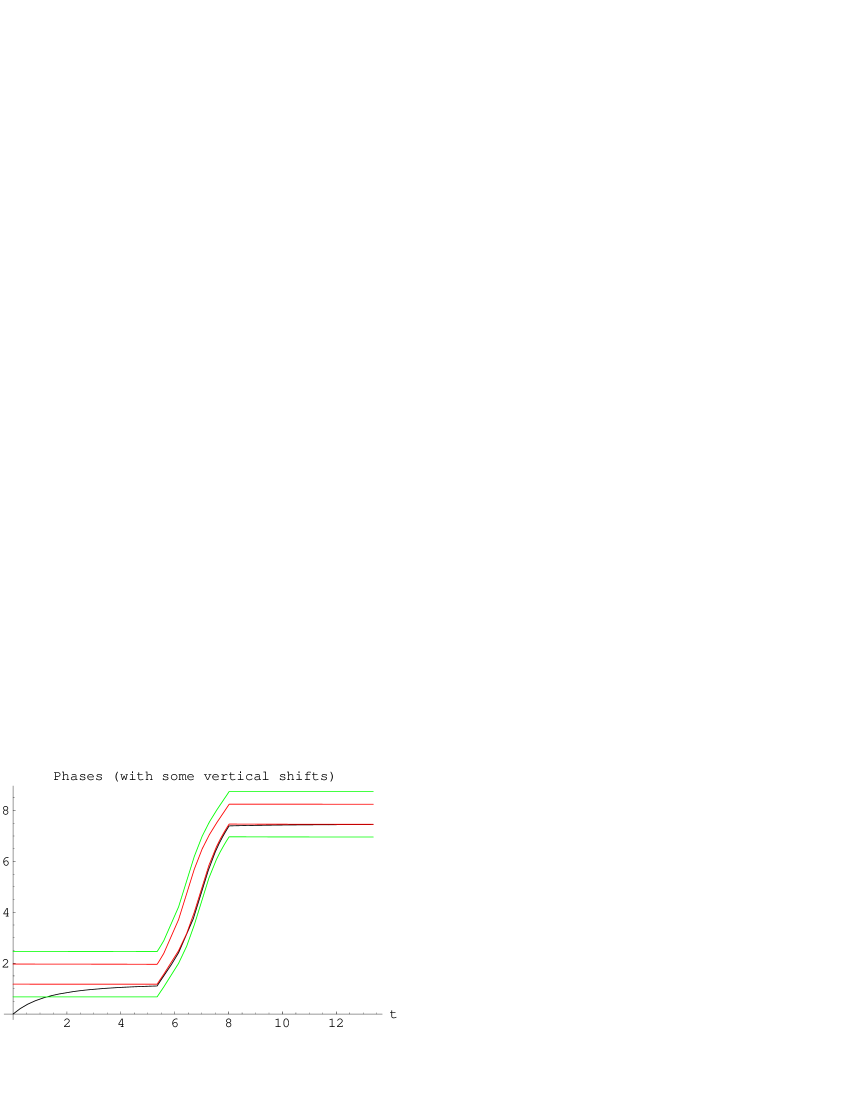
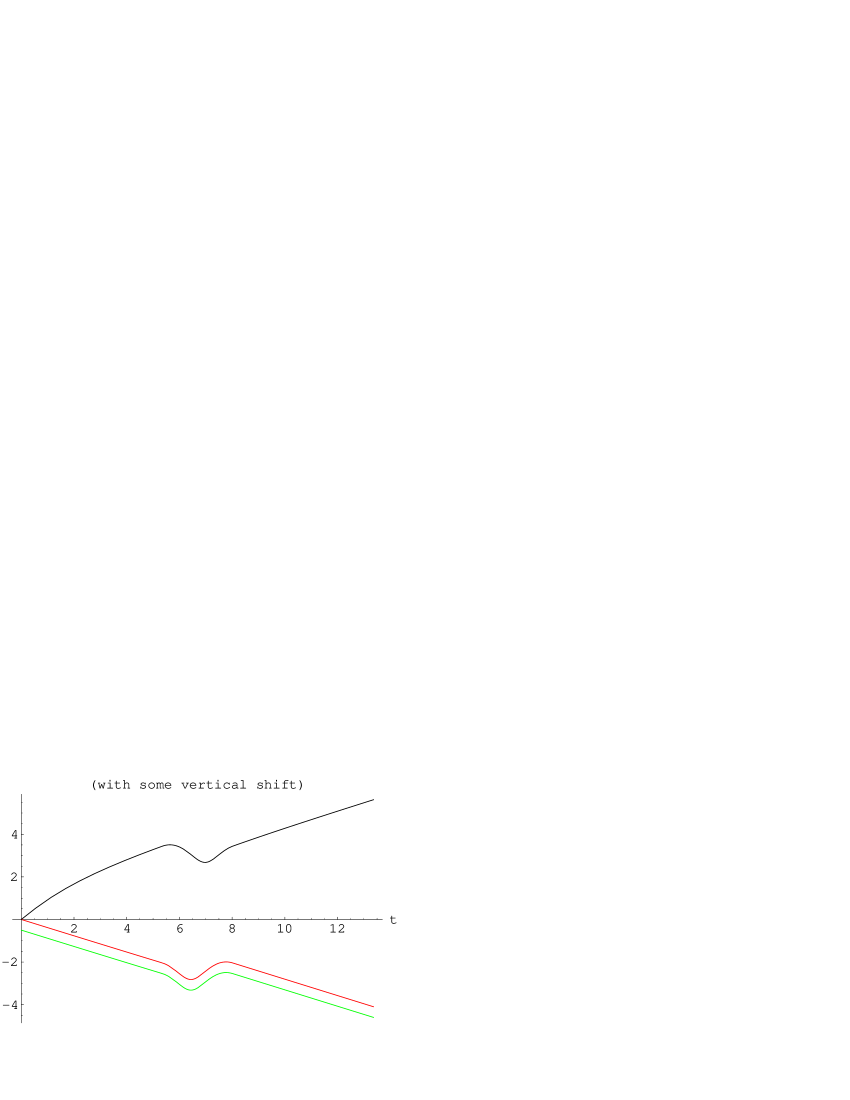
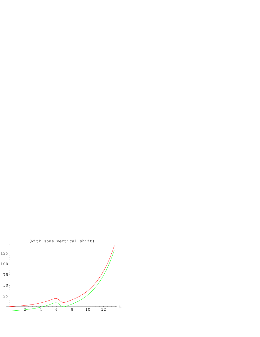
Fig. 7 illustrates the above statements. Here the top panels contain the plots of the two different solutions of Eq. (9). The bias function $f$ is the same sequence of periodically repeated rectangular pulses which was used above, see the inset in Fig. 6, the only difference is the constant constituent which now amounts to $\iota_{\mbox{\scriptsize dc}}=1.45$ (it is worth reminding also that now $\beta=0$). The phase function of the first period phase evolution, starting at the coordinate origin, is considered as the ‘ground’ solution of Eq. (9) denoted above as $\phi_{0}$. It is plotted at the top-left panel. In the lower-left panel, the integrals $P_{0},Q_{0}$ calculated from $\phi_{0}$ are plotted. The top-right panel displays the ‘continuation’ of $\phi_{0}$ to the second period $[T,2T]$ which, afterwards, is returned (‘shifted’ to the left by $T$) to the $\phi_{0}$ domain. (No ‘vertical’ shift is here applied.) As it had been mentioned above, due to the periodicity of $f(t)$, the ‘shifted’ solution is again a solution of Eq. (9). We denote it $\phi(t)$. (This function is distinguished by the specific initial condition $\phi(0)=\phi_{0}(T)$ which however plays no role in the current context.) Finally, the graph displayed in the lower-right panel is the result of straightforward computation of $C\equiv C[\phi,\phi_{0}]({t})$ in accordance with definition (13) and (12). More exactly, the deviation of $C$ off its averaged (on the interval $[0,T]$) value which is $\approx$$-0.406445$ is shown.

One sees that the functional $C=C[\phi,\phi_{0}](t)$ computed ‘from the first principles’ is, after all, a constant up to a small deviation. The latter irregularly oscillates around zero with the amplitude which is at least 6 orders less than the phase magnitudes. It represents the ‘numerical noise’ reflecting mostly tolerable inaccuracy of approximate numerical solutions of differential equation.

Figure 7: The top-left and top-right panels display the phase functions $\phi_{0}({t})$, $\phi({t})$, respectively, verifying Eq. (9). At the lower-left panel, the integrals $P_{0}({t})$ (the red curve) and $Q_{0}({t})$ (the green curve) are plotted, see Eqs. (10), (11). The deviation of $C[\phi,\phi_{0}]({t})$ computed in accordance with Eqs. (13), (12) from its average value is displayed at the lower-right panel.

The closely related computation displayed in Fig.  8 illustrates the application of Eq. (18) for the generating of new solutions of Eq. (9) from a known one. Here the black curve shows the ‘ground’ solution, $\phi_{0}$, starting in the coordinate origin; note that any other phase function might be used instead. Then we chose, say, $C=0.2$ and compute $\phi({t})$ by means of Eq. (18). The result is represented by the red curve which was shifted downward by 0.1 units for the convenience of further visual collations. Next, we carry out the straightforward numerical integrating of Eq. (9) adopting the same initial conditions $\phi|_{{t}=0}=\phi(0)$ as the just generated solution obeys. The green curve represents the result of the integrating which is also additionally shifted downward, here by 0.2 units. Finally, the blue graph is the difference of the results of computation of the same phase function by these two methods (viz the application of Eq. (18) and the numerical ODE integrating) magnified by the factor of $0.5\times 10^{6}$. Again, one sees that Eq. (18) ensures the stable accuracy about six true decimal digits with the discrepancy falling in the level of ‘numerical noise’.

Figure 8: The black curve represents the ‘ground’ phase function. The red and green curves are the phase functions (shifted downward by 0.1 and 0.2 units, respectively) which are computed in different ways: the red curve is obtained by means of Eq. (18) for $C=0.2$ while the green one is the result of numerical integration of Eq. (9) with the same initial conditions as the ‘red’ solution obeys. Finally, the blue curve shows the difference of the “red” and “green” functions magnified by the factor of $0.5\times 10^{6}$.

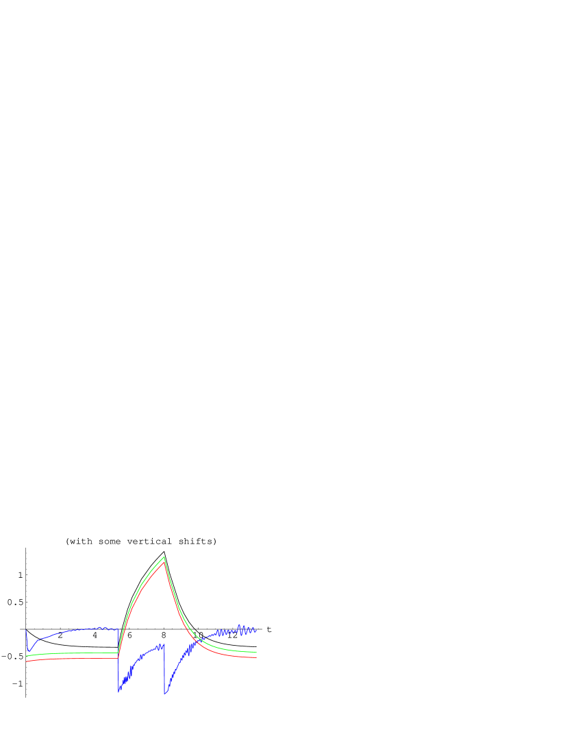
It is important to note that, in the relationships above, the roles of the functions $\phi_{0}$ and $\phi$ (any two solutions of Eq. (9)) should be symmetric by general reasons. However Eq. (18) does not reveal, apparently, such a symmetry since it involves the integrals $P_{0}$, $Q_{0}$ determined by the solution $\phi_{0}$ but no similar contribution connected with $\phi$ is present. Besides, Eq. (18) is easily solvable with respect to $\phi$ but represents to a nonlinear integral equation with respect to $\phi_{0}$.

Any inconsistency does not arises here however and the asymmetry mentioned above is actually a fallacious one. The point is that there is a specific algebraic relation which constrains $P$- and $Q$-functionals associated with any two solutions of Eq. (9). It enables one, in particular, to represent any $P,Q$ as a simple elementary function of another $P,Q$-pair. Namely, the following remarkable relation takes place.

Proposition 2

Let $\phi_{0}({t})$, $\phi({t})$, $P_{0}({t})$, $Q_{0}({t})$ be as in Proposition 1. Let also $P({t})$, $Q({t})$ be determined from $\phi({t})$ in the same way as $P_{0}({t})$, $Q_{0}({t})$ are determined from $\phi_{0}({t})$. Then

$$Q+\mathrm{i}e^{-P}={(Q_{0}+\mathrm{i}e^{-P_{0}})-C\over 1+C(Q_{0}+\mathrm{i}e^{-P_{0}})}$$ (22)

with the same real constant $C$.

Remarks:

• Inverting (22), one gets the alike formula

  $$Q_{0}+\mathrm{i}e^{-P_{0}}={(Q+\mathrm{i}e^{-P})+C\over 1-C(Q+\mathrm{i}e^{-P})}$$ (23)

  which differs from (22), apart of interchanged roles of $P,Q$ and $P_{0},Q_{0}$, by the opposite sign of the $C$-constant alone.

• From viewpoint of the induced transformation group structure, the transformation (22) coincides with the relativistic velocity addition rule.

• In view of the relationship above, it seems natural to incorporate the real-valued functions $P({t})$, $Q({t})$ into the complex-valued one defined as follows:

  $${\cal F}({t})=Q(t)+\mathrm{i}e^{-P(t)}.$$ (24)

  Then the transformation described Eq. (22) may be named, in a sense, meromorphic since ${\cal F}$ is expressed via ${\cal F}_{0}$ as a (meromorphic) function of ${\cal F}_{0}$.

• The definition of $P,Q$-integrals by (10), (11)-like equations is equivalent to the equation

  $${\mathbin{\mathrm{d}}\over\mathbin{\mathrm{d}}t}{\cal F}(t)=-\mathrm{i}e^{\mathrm{i}\phi(t)}\Im{{\cal F}(t)}.$$ (25)

  Indeed, rewriting it as ${\mathbin{\mathrm{d}}(\Re{\cal F})/\mathbin{\mathrm{d}}t}+\mathrm{i}{\mathbin{\mathrm{d}}(\Im{\cal F})/\mathbin{\mathrm{d}}t}=(\sin\phi-\mathrm{i}\cos\phi)(\Im{\cal F})$ and separating the pure imaginary part, one gets ${\mathbin{\mathrm{d}}(\Im{\cal F})/\mathbin{\mathrm{d}}t}=-\cos\phi\cdot\Im{\cal F}$, which, for nonzero $\Im{\cal F}$, yields $\Im{\cal F}=\exp(-\int\cos\phi\mathbin{\mathrm{d}}\phi)$, i.e. in accordance with definition (24), Eq. (10) in fact. Next, separating the real part, one gets ${\mathbin{\mathrm{d}}(\Re{\cal F})/\mathbin{\mathrm{d}}t}=\sin\phi\cdot\Im{\cal F}$. Integrating it and taking into account the representation of $\Im{\cal F}$ just obtained, one gets Eq. (11).$\square$

• Working in terms of $\cal F$ instead of $P,Q$, the choice of $t=0$ as the lower integral limit in (10), (11), is equivalent to the initial condition

  $${\cal F}(0)=\mathrm{i}$$ (26)

  for the function ${\cal F}$ verifying Eq. (25).

• Inverting Eq. (22), ${\cal F}_{0}$ can be represented as a function of ${\cal F}$ (see (23)). Then Eq. (9) can be solved with respect to $\phi_{0}(t)$ which is represented as explicit function of $\phi(t)$, $P({t})$, $Q({t})$ (and $C$) as follows

  $$e^{\mathrm{i}\phi_{0}({t})} = e^{\mathrm{i}\phi({t})}{1-C(Q-\mathrm{i}e^{-P})\over 1-C(Q+\mathrm{i}e^{-P})},$$ (27)

  The dual Eqs. (18),(19) manifest the symmetric role of the two solutions $\phi,\phi_{0}$ noted above.

Proposition proof. The relationship to be proven belongs to the category of ones for which, as the true formula is recorded, the proof reduces to a straightforward computation. Indeed, let us rewrite Eq. (18) as follows

$$e^{\mathrm{i}\phi(t)}=e^{\mathrm{i}\phi_{0}(t)}{1+C\overline{{\cal F}_{0}}\over 1+C{{\cal F}_{0}}}$$ (28)

and calculate the $t$-derivative of the difference

$$\delta\equiv{\cal F}-{{\cal F}_{0}-C\over 1+C{\cal F}_{0}}={\cal F}-{1\over C}+{1+C^{2}\over C(1+C{\cal F}_{0})}.$$

Then the straightforward computation yields

$${\mathbin{\mathrm{d}}\delta\over\mathbin{\mathrm{d}}t} = {\mathbin{\mathrm{d}}{\cal F}\over\mathbin{\mathrm{d}}t}-{1+C^{2}\over(1+C{\cal F}_{0})^{2}}{\mathbin{\mathrm{d}}{\cal F}_{0}\over\mathbin{\mathrm{d}}t}$$

$$= \mbox{\scriptsize$1\over 2$}e^{\mathrm{i}\phi}(\overline{\cal F}-{\cal F})-\mbox{\scriptsize$1\over 2$}{1+C^{2}\over(1+C{\cal F}_{0})^{2}}e^{\mathrm{i}\phi_{0}}(\overline{\cal F}_{0}-{\cal F}_{0})$$

$$= \mbox{\scriptsize$1\over 2$}e^{\mathrm{i}\phi_{0}}\left({1+C\overline{{\cal F}_{0}}\over 1+C{{\cal F}_{0}}}(\overline{\cal F}-{\cal F})-{1+C^{2}\over(1+C{\cal F}_{0})^{2}}(\overline{\cal F}_{0}-{\cal F}_{0})\right).$$

The following identity takes place

$$\overline{\cal F}-{\cal F} = \overline{\delta}-{\delta}-{1+C^{2}\over C}\left(\overline{1\over 1+C{\cal F}_{0}}-{1\over 1+C{\cal F}_{0}}\right)$$

$$= \overline{\delta}-{\delta}+{1+C^{2}\over({1+C{\cal F}_{0}}){(1+C\overline{\cal F}_{0})}}(\overline{{\cal F}_{0}}-{\cal F}_{0}).$$

It implies, together with the equation just derived, the following series of equalities:

$${\mathbin{\mathrm{d}}\delta\over\mathbin{\mathrm{d}}t} = \mbox{\scriptsize$1\over 2$}e^{\mathrm{i}\phi_{0}}\left({1+C\overline{{\cal F}_{0}}\over 1+C{{\cal F}_{0}}}\left(\overline{\delta}-{\delta}+{1+C^{2}\over({1+C{\cal F}_{0}}){(1+C\overline{\cal F}_{0})}}(\overline{{\cal F}_{0}}-{\cal F}_{0})\right)\right.$$

$$\left.\hskip 21.52771pt-{1+C^{2}\over(1+C{\cal F}_{0})^{2}}(\overline{\cal F}_{0}-{\cal F}_{0})\right)$$

$$= \mbox{\scriptsize$1\over 2$}e^{\mathrm{i}\phi_{0}}\left({1+C\overline{{\cal F}_{0}}\over 1+C{{\cal F}_{0}}}(\overline{\delta}-{\delta})+{1+C\overline{{\cal F}_{0}}\over 1+C{{\cal F}_{0}}}{1+C^{2}\over({1+C{\cal F}_{0}}){(1+C\overline{\cal F}_{0})}}(\overline{{\cal F}_{0}}-{\cal F}_{0})\right.$$

$$\left.\hskip 21.52771pt-{1+C^{2}\over(1+C{\cal F}_{0})^{2}}(\overline{\cal F}_{0}-{\cal F}_{0})\right)$$

$$= \mbox{\scriptsize$1\over 2$}e^{\mathrm{i}\phi_{0}}{1+C\overline{{\cal F}_{0}}\over 1+C{{\cal F}_{0}}}(\overline{\delta}-{\delta}).$$

The last equation is equivalent to the system of two linear homogeneous first order ODEs for the two (real valued) functions $\Re\delta,\Im\delta$. Moreover, in accordance with standard ‘normalization’ (26) and $\delta$ definition, one has

$$\delta(0)=0,$$

the null initial condition. Thus $\delta(t)\equiv 0$, i.e. one gets the equation

$${\cal F}={{\cal F}_{0}-C\over 1+C{\cal F}_{0}}$$ (29)

which is nothing but Eq. (22). $\square$

Thus, in accordance with the remarks above, we may consider the expression (13) as the functional over the set of pairs of solutions of Eq. (9) (the direct square of the solution set) taking it onto the real axis. To be more exact, since the limiting case $C\rightarrow\infty$ is quite legitimate, one has to replenish the real axis by the infinitely remote point. The result is the circumference but it appears here as the isomorphic image of the real projective line $RP^{1}$ which is just the natural ‘index space’ to be used for the ‘enumerating’ of solutions of Eq. (9). Specifically, having fixed some $\phi_{0}$, the inverse map from $S^{1}\simeq RP^{1}$ onto the first factor in the direct product yields the (1-1 non-canonical) parameterization of the space of solutions by the circumference points.

It is worth noting that the $C$-map (13), (12) is antisymmetric with respect to the interchange of the functional arguments $\phi,\phi_{0}$, i.e.

$$C[\phi,\phi_{0}]=-C[\phi_{0},\phi].$$ (30)

The property (30) can be established as follows. Eq (14) implies

$$e^{P_{0}}{dC[\phi,\phi_{0}]^{-1}\over d\,{t}}=2\mathrm{i}(\zeta-\zeta_{0})^{-2}(\zeta_{0}D[\zeta]-\zeta D[\zeta_{0}])=-e^{P}{dC[\phi_{0},\phi]^{-1}\over d\,{t}}$$

and therefore $C[\phi_{0},\phi]$ is automatically a constant, provided $C[\phi,\phi_{0}]$ is. Further, in accordance with (21) the equality $-C[\phi_{0},\phi]=C[\phi,\phi_{0}]$ takes place for $t=0$. Hence these constants coincide up to the opposite signs and (30) holds everywhere.

Proposition 3

If $\phi,\phi_{0}$ are solutions of Eq (9) then Eq. (30) is satisfied. $\square$

Phase-locking and its necessary condition

Now let us consider the implications of the above relationships in application to the property of the phase-locking. The latter is connected with the specific asymptotic behavior of the phase functions $\phi({t})$ verifying, in our case, Eq. (9). Namely, in the case of phase-locking Eq. (6) has to be satisfied, asymptotically.

To describe efficiently this property, let us define the sequence of functions $\phi_{j}(t)$ defined on the segment $[0,T]$ as follows

$$\phi_{j}({t})=\phi({t}+jT)-2\pi[[\phi(jT)/2\pi]],\;j=0,1,2,3\dots,\;{t}\in{}[0,T]$$ (31)

where the double brackets $[[\dots]]$ stands for the integer part of the real number enclosed. Thus the plot of $\phi_{j}({t})$ displays how the ‘genuine’ phase function $\phi({t})$ looks like ‘on the $j$’th segment’ of the length (duration) $T$ with respect to the closest level aliquot to $2\pi$. To that end, its graph is shifted downward or upward by such a number of ‘full phase revolutions’ $2\pi$ which returns its left-boundary point $\phi_{j}(0)$ to the segment $[0,2\pi)$.

We have already used such a trick in the arrangement of plots of phase functions calling it occasionally ‘the segmenting’. Here the explicit transformation of the phase function on the corresponding t-segments of duration $T$ yielding a specific sequence of the phase functions defined on the segment $[0,T]$ is introduced.

All the functions $\phi_{j}$ satisfy Eq. (9). The specific (and characteristic) property of the sequence of its solutions $\phi_{j}$’s associated with a single solution $\phi$ defined for all $t$ is obviously the following:

$$\phi_{j+1}(0)=\phi_{j}(T)\mbox{\ mod $2\pi$},\phi_{j}(0)\in[0,2\pi),j=0,1,2\dots$$ (32)

Given the sequence $\{\phi_{j}\}$ of solutions of Eq. (9) on the segment $[0,T]$ fulfilling the condition (32), the valid phase function $\phi(t),t\in[0,\infty),$ can be reconstructed in the obvious way.

It is convenient to represent the phase-locking property in terms of properties of the functional sequence $\phi_{j}$. It can be stated the following:

In the case of phase-locking the sequence $\phi_{j}$ uniformly converges on the segment $[0,T]$ to some limiting function

$$\phi_{\infty}({t})=\lim_{j\rightarrow\infty}\phi_{j}({t})$$ (33)

which satisfies Eq. (9) and the condition

$$\phi_{\infty}(T)=\phi_{\infty}(0)+2\pi k\Leftrightarrow e^{\mathrm{i}\phi_{\infty}(T)}=e^{\mathrm{i}\phi_{\infty}(0)}$$ (34)

for some integer k.

It is natural to select and fix the ‘ground’ specimen of phase functions denoting it $\phi_{0}({t})$ , ${t}\in{}[0,T],$ characterizing it by means of the null initial value $\phi_{0}(0)=0$ (the symbol $\phi_{(0)}({t})$ and its derivates will be also used in cases prone of confusion with the notation introduced in (31)). Having posed the problem in such a way, $\phi_{0}({t})$ is completely determined by the bias function $f({t})$. We also assume the value ${t}=0$ to be the lower integration boundary for the integrals in the $P_{0},Q_{0}$ definitions (10),(11). Then Eq. (18) implies that there exists a constant $C_{\infty}$ such that

$$e^{\mathrm{i}\phi_{\infty}({t})}=e^{\mathrm{i}\phi_{0}({t})}{1+C_{\infty}(Q_{0}({t})-\mathrm{i}e^{-P_{0}({t})})\over 1+C_{\infty}(Q_{0}({t})+\mathrm{i}e^{-P_{0}({t})})}.$$ (35)

(We assume $C_{\infty}$ to be finite but the case of ‘infinite $C_{\infty}$’ is also tractable, with minor modifications, in the same way.) Taking the above representation of $e^{\mathrm{i}\phi_{\infty}({t})}$ into account, it is easy to see that Eq. (34) is satisfied if and only if the equation

$$C_{\infty}^{2}\times(Q_{0}(T)\cos\mbox{\scriptsize$1\over 2$}\phi_{0}(T)+e^{-P_{0}(T)}\sin\mbox{\scriptsize$1\over 2$}\phi_{0}(T))$$

$$\hbox to0.0pt{\hss+}C_{\infty}\times(Q_{0}(T)\sin\mbox{\scriptsize$1\over 2$}\phi_{0}(T)+(1-e^{-P_{0}(T)})\cos\mbox{\scriptsize$1\over 2$}\phi_{0}(T))$$

$$\hphantom{C_{\infty}}+\sin\mbox{\scriptsize$1\over 2$}\phi_{0}(T)=0$$ (36)

admits a real root $C_{\infty}$. In turn, the latter condition is equivalent to the inequality

$$\Delta[f] \equiv -Q_{0}(T)(e^{-P_{0}(T)}+1)\sin\phi_{0}(T)$$

$$-\mbox{\scriptsize$1\over 2$}\left(-Q_{0}(T)^{2}+\left(e^{-P_{0}(T)}+1\right)^{2}\right)(1-\cos\phi_{0}(T))$$

$$+(1-e^{-P_{0}(T)})^{2}$$

$$\equiv 4e^{-P_{0}(T)}\times$$

$$\left(\left[-\mbox{\scriptsize$1\over 2$}e^{\mbox{\scriptsize$1\over 2$}P_{0}(T)}Q_{0}(T)\sin\mbox{\scriptsize$1\over 2$}\phi_{0}(T)+\cosh\mbox{\scriptsize$1\over 2$}{}P_{0}(T)\cos\mbox{\scriptsize$1\over 2$}\phi_{0}(T)\right]^{2}-1\right)$$

$$\geq 0$$ (38)

$$\Leftrightarrow \left|\cosh\mbox{\scriptsize$1\over 2$}P_{0}(T)\cos\mbox{\scriptsize$1\over 2$}\phi_{0}(T)-\mbox{\scriptsize$1\over 2$}e^{\mbox{\scriptsize$1\over 2$}P_{0}(T)}Q_{0}(T)\sin\mbox{\scriptsize$1\over 2$}\phi_{0}(T)\right|\geq 1.$$ (39)

The above is therefore the necessary condition of phase-locking. It reflects in fact the property of the very function $f$.

As we shall show, the similar but strict inequality is the sufficient condition of the phase-locking for the phase function described by Eq. (9). (In the case of the equality, the convergence to some asymptotic limit is observed as well but it is slower and reveals some other specialities.) The vantage of such a form of the phase-locking ‘monitoring’ is that this is the asymptotic property manifesting itself for sufficiently large $t$. Generally speaking, one cannot forecast in advance how long phase evolution has to be tracked for the detection of the corresponding $T$-scale reproducibility of the phase function form which would make evidence of the phase-locking. On the other hand, making use of the condition (39), the appearance of phase-locking is deduced directly from the properties of a single solution of Eq. (9) computed on the finite interval $[0,T]$.

More on the role of the discriminant $\Delta[f]$

The function $\Delta\equiv\Delta[f]$ plays an important role in the problem of description of asymptotic properties of solutions of Eq. (9). We may interpret it as the functional on the set of bias functions $f$ since the functions $\phi_{0},P_{0},Q_{0}$ from which it is built upon are uniquely determined by $f$: $\phi_{0}$ is the solution of Eq. (9) with initial condition $\phi_{0}(0)=0$, $P_{0},Q_{0}$ are calculated from $\phi_{0}$ in accordance with Eqs. (10), (11) and the initial conditions $P_{0}(0)=0,Q_{0}(0)=0.$ One may also choose $f$ to belong to some more restricted class of functions, for example, a family parameterized by a finite set of parameters. Then, one may also regard $\Delta$ as the function of these parameters and study its properties.

Adopting the last interpretation, Fig. 9 shows $\Delta$ as the function of a single variable, the constant bias constituent $\iota_{\mbox{\scriptsize dc}}$, assuming the very bias function to be the periodic sequence of rectangular pulses shown in the inset in Fig. 6.

One recognizes the three minima on the fragment of the $\Delta$ plot seated in Fig. 9, the left one situating very close to the horizontal coordinate axis and the middle one being fairly steep. More narrowly, the minima above are shown in Fig. 10, where the plots of their vicinities are displayed with higher resolutions. One sees that in all the three cases the minima lay well below the horizontal coordinate axes. Hence each of them is encompassed by some $\iota_{\mbox{\scriptsize dc}}$ segment where $\Delta$ assumes negative values (and this is the universal property: there are no positive minima of $\Delta$). These are separated by segments where $\Delta$ is positive.

Figure 9: The dependence of the discriminant $\Delta$ on the constant constitution $\iota_{\mbox{\scriptsize dc}}$ of the bias with the other parameters held fixed.

Figure 10: Separate representations of vicinities of the minima observed on the graph shown in Fig. 9 are given with higher plot resolutions.

As we shall show, each segment of positive $\Delta$ determines the area of the values of the parameter $\iota_{\mbox{\scriptsize dc}}$ giving rise to the phase-locking phase evolution of a common order. Such segments are directly associated with so called Shapiro steps — strictly constant voltage segments observed on the Josephson junction I-V curve [6, 4]. In particular, the domain of $\iota_{\mbox{\scriptsize dc}}$ values shown in Fig. 9, where $\Delta>0$, contain the steps of the orders, from left to right, $-1$ (extending to the left beyond the plot boundary), 0, 1, and 2.

The values of $\iota_{\mbox{\scriptsize dc}}$ falling into the segments of negative $\Delta$ correspond to the apparently ‘irregular’ behavior of the phase which is similar to one displayed in Fig. 5. We shall see however that these phase evolutions do not correspond to an actual chaos (pseudo-chaos) [5]. Rather, these are the manifestations of a ‘beating’ produced by two inconsonant frequencies. In particular, such phase evolutions imply quite definite average voltages which are obtained by the averaging of (5) over large time intervals. This point will be considered in more details later on.

Unstable and stable phase-locking candidates

The algorithm allowing one to reconstruct the phase functions at any moment of time $t$ divides into several steps. At first, one has to solve the quadratic equation (36) with respect to $C$, assuming its roots to be real (that takes place iff $\Delta\geq 0$). Then, if $\Delta>0$, Eq. (18) yields the two phase functions which are the candidates to the role of possessor of the ‘refined’ property of phase-locking (the limiting function asymptotically approximating generic solutions).

A somewhat delicate point is the revealing which of the two solutions is the one we search for. The answer is connected with the stability property (the phase-locking must be stable) and can be provided, in principle, with the help of the standard perturbational analysis (the local stability problem, cf. [5]) which however yield not the actual problem solution but rather a recipe of its computation. Fortunately, there is an attractive opportunity to directly manifest not only the effect of infinitesimal perturbations but, at one blow, to establish the ‘global’ stability property allowing perturbations of arbitrary magnitudes. Here we seize upon it.

Figure 11: The black curve shows the ‘ground’ solution $\phi_{0}$ (starting from the coordinate origin). The two red curves are the the candidates to the role of the asymptotic limiting phase function which are constructed by means of Eqs. (36), (18). The green curves are the phase functions constructed by means of a straightforward numeric integration of (9) obeying the same initial conditions as the ‘red’ solutions; for better clarity, they are shifted, afterwards, in ‘vertical’ direction by 0.5 units upward (the top curve) and downward (the lower curve), the red graphs being undergone no shifts.

Figure 12: The plots display the discrepancies between the phase-locking candidates displayed in Fig. 11 and obtained by means of Eqs. (36), (18) against the ones obtained by means of straightforward numerical integration of Eq. (9) with the same initial conditions as the former functions obey.

This point is illustrated by Fig. 11. Here the black curve shows the ‘ground’ solution $\phi_{0}$ (starting from the coordinate origin) for the rectangular pulse bias of the profile shown in the inset in Fig. 6, and $\iota_{\mbox{\scriptsize dc}}=1.25$ (which yields a positive $\Delta$ value, see Fig. (9)).

The red curves are the graphs of solutions (‘phase-locking candidates’) one of which is expected to realize the ‘refined’, precisely steady phase-locking evolution obeying the property (6) and representing, in a sense, the asymptotic limit of a generic phase function. The phase-locking candidates are constructed by means of Eqs. (18) with the two values of the constant $C$ obtained from Eq.  (18).

The green curves represent the phase functions constructed by means of a straightforward numeric integrations of Eq. (9) obeying the same initial conditions as the ‘red’ solutions does. The plot graphs are afterwards shifted ‘in vertical direction’ by 0.5 units upward (the green top curve) and downward (the lower one) making easier the visual collation of the profiles of the functions involved.

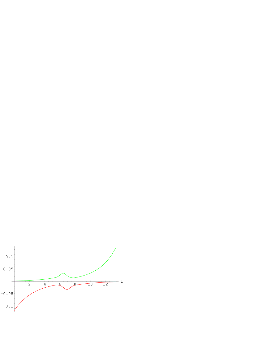
The apparent qualitative coincidence of the results of the two ways of computation of ‘phase-locking candidates’ is numerically confirmed in Fig. 12 where their relative discrepancies are plotted. One sees that the two computations agree at the level one part in $10^{6}$ which is close to the accuracy of the numerical integrating of the ODE involved.

It is natural to suppose that only one of the two solutions shown as the red (or, equivalently, green) curves in Fig. (11) is of interest as a model of physical relevance because another one is necessarily unstable (it plays the own specific role as the separator of two ‘basins’ of the phase-locking in the space of all phase functions, though). Indeed, the distinction of their stability properties is clearly seen in Fig. 13.

Figure 13: The evolution of perturbations of the two candidates the ‘refined’ phase-locking states represented in Fig. 12 by red graphs are displayed, the perturbation function corresponding to the stable evolution (the red graph) being magnified by the factor of $10^{2}$.

Here the evolution of perturbations of the two solutions shown in Fig. 12 (the red curves) is displayed, The perturbed phase functions are defined as the solutions $\phi^{(\varepsilon)}({t})$ to Eq. (9) with initial conditions distinct from the ones the phase-locking candidates obey by amount of 0.1%: $\phi^{(\varepsilon)}(0)=\phi(0)\times(1\pm 0.001)$. For definiteness, we chose $\phi^{(\varepsilon)}(0)=\phi(0)\times(1+0.001)$ for the upper curve in Fig. 12 and $\phi^{(\varepsilon)}(0)=\phi(0)\times(1-0.001)$ for the lower one. Accordingly, the upper (green) graph in Fig. 13 shows $\phi^{(\varepsilon)}({t})-\phi({t})$ for the ‘upper’ phase-locking candidate; it makes evidence of a strong instability since the deviation is permanently (and, in fact, exponentially) growing. On the contrary, the lower (red) curve in Fig. 13 demonstrate the exponential relaxation of the perturbation; moreover, to display it more clearly, the perturbation value displayed is magnified by the factor of $10^{2}$, i.e. the function $100(\phi^{(\varepsilon)}({t})-\phi({t}))$ is actually plotted.

Thus we see that only the lower red curve in Fig. 12 corresponds to a stable phase evolution. The evolution described by another, upper, (red) curve in Fig. 12 related to another solution of Eq. (36), is unstable. As a matter of fact, the first curve describes an attractor of all the ‘neighboring’ solutions while the second one ‘repels’ them.

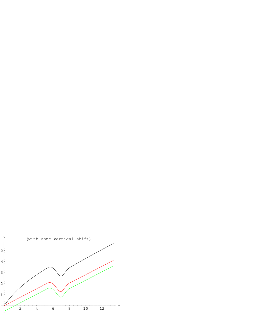
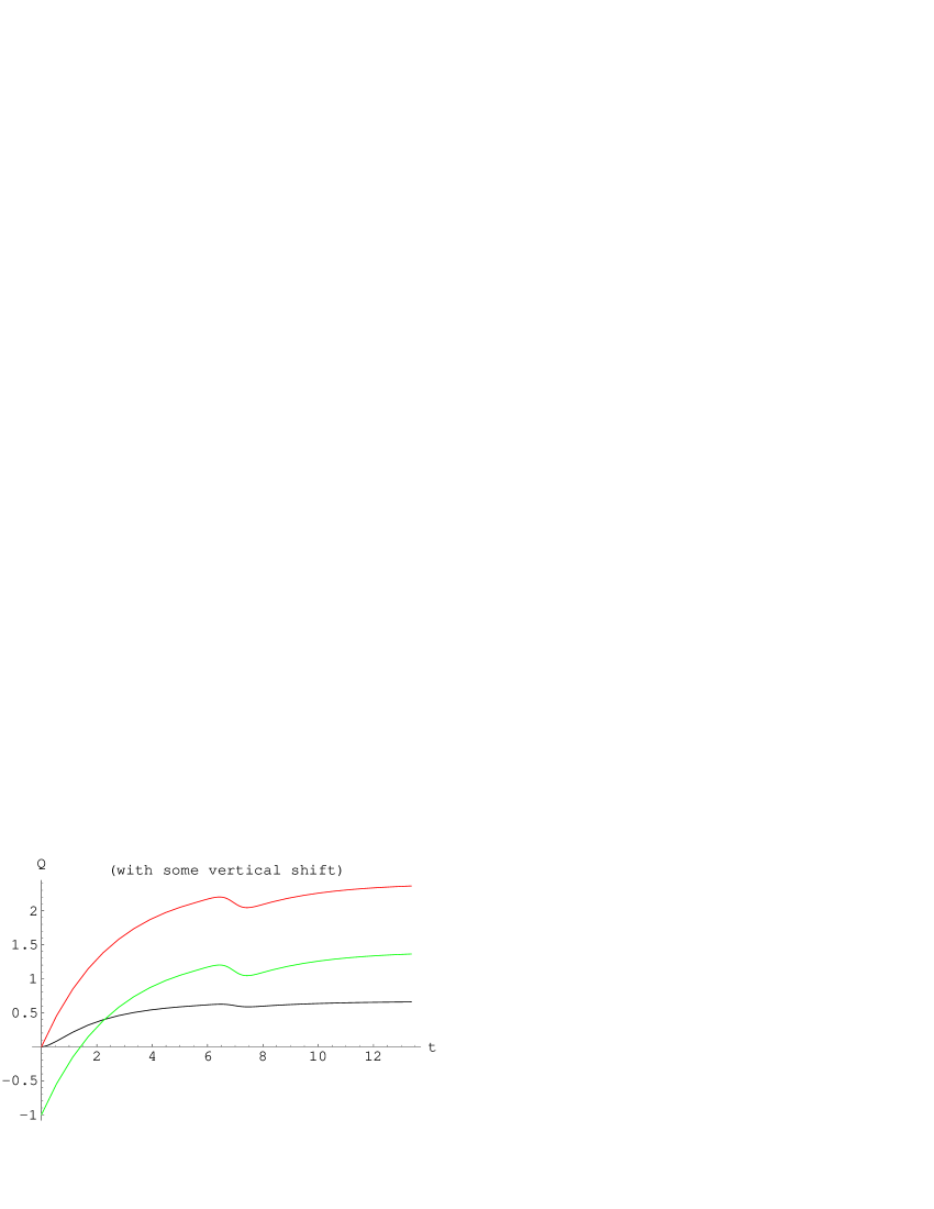
Above, we have numerically demonstrated the validity of the equation (35) allowing one to build a new solution from the known one. Similarly, Eq. (22) allows one to determine, knowing $C$, the integrals $P({t})$ and $Q({t})$ associated with the former. Figures 14 and 16 displays the results of the corresponding computation. There the black curves represent the $P$- and $Q$-integrals corresponding to the ‘ground’ phase function $\phi_{0}$ which is represented by black graph in Fig.  11. The red curves are the integrals for the refined phase-locking candidates which are determined by means of Eq. (35). The green curves (which are shifted in vertical direction downward) are the same functions but they are obtained by straightforward numerical integrating in accordance with $P$ and $Q$ definitions. In Fig. 16, the relative discrepancies of the two ways of computation of the $P$- and $Q$- integrals are displayed. (Note that the relative discrepancy growth observed near the left boundary ${t}=0$ is the numerical artifact caused by the vanishing of $P(0)$ and $Q(0)$.)

Figure 14: $P$-integrals corresponding to the stable steady phase-locking are shown. The black curve is the $P$-integral for the ground phase function $\phi_{0}$ (the black curve in Fig.  11). The red curve represents $P$-integral is associated with the refined phase-locking candidate determined by means of Eq. (35). The green curve represent the same function obtained directly from definition (10), afterwards it being shifted downward by 0.5 units.

Figure 15: $Q$-integrals corresponding to the same stable phase-locking state as in Fig. 14 are shown. The color meaning is the same as therein. The green graph is shifted downward by 1 unit.

Figure 16: The relative discrepancies of the different ways of computation of $P$- and $Q$-integrals (by means of Eq. (35) and the computation in accordance with definitions from the known phase functions) corresponding to the stable phase-locking.

Figure 17: The graphical matter displayed is similar to the one shown in Fig. 14 but it is connected with the unstable steady phase evolution whose phase function is represented by the upper red curve in Fig. 11.

Figure 18: Similar to Fig. 15 but corresponds to the unstable phase-locking candidate. The ‘ground’ $Q$-integral corresponding to the ‘ground’ phase function (the analogue to the black graph in Fig. 17) is not shown because of the too large distinction in the magnitudes.

Figure 19: The relative discrepancies of the results of two different ways of computation of $P$- and $Q$-integrals corresponding to the unstable phase-locking candidate.

$T$-scale discretization of the phase evolution

As it has been noted, any phase function $\phi({t})$ defined on arbitrary $t$ domain can be equivalently described by the sequence of the functions $\phi_{j}({t})$ defined on the common interval $[0,2\pi]$, see Eq. (31). At the same time, as a solution of Eq. (9), each function $\phi_{j}({t})$ can be represented in the form (16) for the own specific value of the constant $C$ which we denote $C_{j}$. A simple but important observation reads:

The property of phase-locking equivalent to the existence of the limit $\phi_{\infty}({t})$ of the sequence of functions $\phi_{j}({t})$ (see Eq. (33)) associated with a generic solution of Eq. (9), is also equivalent to the existence of the limit $C_{\infty}$ of the sequence of real constants $C_{j}$, connected with $\phi_{j}$, either finite or infinite.

Thus

$$C_{\infty}=\lim_{j\rightarrow\infty}C_{j}$$ (40)

must exist, either finite or infinite, provided the phase-locking takes place.

On the contrary, the phase-locking does not arise and the phase function reveals apparently ‘irregular’ behavior if and only if the sequence $C_{j}$ has no limit.

Remark:

Allowing constants $C_{j}$ and their limit to assume infinite values, the real projective line $RP^{1}$ isomorphic to the circumference has to be adopted as the space of their ($C$-constants) originating. This can be realized by means of identifying each $C_{j}$ with the pair $(C_{j},1)$ and the interpreting the latter as homogeneous coordinates on $RP^{1}$. The limit of the sequence $C_{j}$ has also to be understood as a point in $RP^{1}$.

Figure 20: The sequence of converging $C_{j}$ which indicates the phase-locking property is shown. The bias is the same periodic rectangular pulse sequence as above besides the specific value of the DC contribution $\iota_{\mbox{\scriptsize dc}}=1.46$.

Figure 21: Here the sequence $C_{j}$ not tending to an apparent limit indicates the absence of the phase-locking (‘irregular’ phase behavior). The bias is the same periodic rectangular pulse sequence as above besides the specific value of the DC contribution $\iota_{\mbox{\scriptsize dc}}=1.40$.

Figures 20, 21 display the two examples of $C$-sequences for the phase-locking (Fig. 20) and ‘irregular’ (Fig. 21) phase evolutions, respectively. The distinction arises because to the slightly different values of the constant bias parameter: $\iota_{\mbox{\scriptsize dc}}=1.46$ for Fig. 20, and $\iota_{\mbox{\scriptsize dc}}=1.4$ for Fig. 21, cf. the left-lower panel of Fig. 10. The other parameters of the bias function $f$ are the same as for the pulse shown in the inset in Fig. 6.

In order to detect the phase-locking without a plain phase simulation, one may, in spite of determination of the constants $C_{j}$ from the functions $\phi_{j}({t})$ by means of Eq. (20), make use of the following recurrence relation which can be derived from Eqs. (31), (32), (18) and $C_{j}$ definition:

$$C_{j+1}={C_{j}\left(e^{-\mbox{\scriptsize$1\over 2$}P_{(0)}(T)}\cos\mbox{\scriptsize$1\over 2$}\phi_{(0)}(T)-Q_{(0)}(T)e^{\mbox{\scriptsize$1\over 2$}P_{(0)}(T)}\sin\mbox{\scriptsize$1\over 2$}\phi_{(0)}(T)\right)-e^{\mbox{\scriptsize$1\over 2$}P_{(0)}(T)}\sin\mbox{\scriptsize$1\over 2$}\phi_{(0)}(T)\over C_{j}\left(e^{-\mbox{\scriptsize$1\over 2$}P_{(0)}(T)}\sin\mbox{\scriptsize$1\over 2$}\phi_{(0)}(T)+Q_{(0)}(T)e^{\mbox{\scriptsize$1\over 2$}P_{(0)}(T)}\cos\mbox{\scriptsize$1\over 2$}\phi_{(0)}(T)\right)+e^{\mbox{\scriptsize$1\over 2$}P_{(0)}(T)}\cos\mbox{\scriptsize$1\over 2$}\phi_{(0)}(T)}$$ (41)

(It is worth reminding that the subscript ‘₍₀₎’ hints at the specific initial conditions the functions $\phi_{(0)},P_{(0)},Q_{(0)}$ obey which read $\phi_{(0)}(0)=0,P_{(0)}(0)=0,Q_{(0)}(0)=0.$ It emphasizes the distinction of the ‘ground’ solution and its derivates from the particular element $\phi_{0}$ of the sequence $\phi_{j}$; we shall omit this notation complication whenever possible.) The relation above is of a notable importance allowing one to obtain, finally, the exhaustive description of the long-term phase behavior on the time scales exceeding $T$ by means of pure algebraic manipulations.

To that end, one has to mention that the map $C_{j}\rightarrow C_{j+1}$ implied by Eq. (41) is fraction linear. It is well known that any such transformation is equivalent to a linear automorphism on a projective space. To make use of much simplification following from such a linear reduction of the problem, let us consider the vector space of 2-element columns $\mathbf{C}=\left[{a\atop b}\right]$ (using here and below boldface characters for notation of matrix-valued quantities) with the ratio of the elements equal to $C$, $a/b=C$. We consider the columns differing by a non-zero multiplier as equivalent, $\left[{a\atop b}\right]\sim\left[{Aa\atop Ab}\right],A\not=0$. Let us also introduce the $2\times 2$ matrix

$$\mathbf{\Phi}=\left(\begin{array}[]{cc}e^{-\mbox{\scriptsize$1\over 2$}P_{0}(T)}\cos\mbox{\scriptsize$1\over 2$}\phi_{0}(T)-Q_{0}(T)e^{\mbox{\scriptsize$1\over 2$}P_{0}(T)}\sin\mbox{\scriptsize$1\over 2$}\phi_{0}(T)&-e^{\mbox{\scriptsize$1\over 2$}P_{0}(T)}\sin\mbox{\scriptsize$1\over 2$}\phi_{0}(T)\\ e^{-\mbox{\scriptsize$1\over 2$}P_{0}(T)}\sin\mbox{\scriptsize$1\over 2$}\phi_{0}(T)+Q_{0}(T)e^{\mbox{\scriptsize$1\over 2$}P_{0}(T)}\cos\mbox{\scriptsize$1\over 2$}\phi_{0}(T)&+e^{\mbox{\scriptsize$1\over 2$}P_{0}(T)}\cos\mbox{\scriptsize$1\over 2$}\phi_{0}(T)\end{array}\right)$$ (42)

which is, as a straightforward check shows, unimodular, $\det\mathbf{\Phi}=1$. Then it is also straightforward to show that the transformation

$$\mathbf{C}_{j+1}=\mathbf{\Phi}\mathbf{C}_{j}.$$ (43)

is equivalent to Eq. (41). The map $\mathbf{C}_{j}\mapsto\mathbf{C}_{j+1}$ corresponding to Eq. (43) is just the linear automorphism of the real projective line $RP^{1}$ mentioned above.

Since the transformation associated with matrix $\mathbf{\Phi}$ does not depends on $j$, starting from $j=0$, after $j-1$ iterations one comes to the equation

$$\mathbf{C}_{j}=\mathbf{\Phi}^{j}\mathbf{C}_{0}.$$ (44)

It is convenient to chose $\mathbf{C}_{0}=\left[{C_{0}\atop 1}\right]$. The very ‘starting’ $C$-constant $C_{0}$ encodes the initial value of the phase function $\phi(t)$. Giving $\phi(0)$, it can be calculated by means of Eq. (20).

Eq. (44) is, essentially, the desirable algebraic relationship describing the long-term phase evolution. The time variable $t$ is here encoded in the integer variable $j$ playing role of a discrete time on the scale $T$ and amounting, numerically, to the integer part of $t/T$.

We shall derive below the expanded version of (44) where the power of the operator $\mathbf{\Phi}$ is given in explicit form.

The ‘irregular’ phase evolution

We consider, first, the case of ‘irregular’ phase evolution when the discriminant $\Delta$, Eq. (38), is negative. In this case we proceed with the problem of calculation of the accumulated phase variation over a long time interval (the single period averaging does not yield a meaningful result here). In accordance with (5), it immediately yields us the value of the average voltage across the junction, i.e. the physically measurable quantity. In particular, we shall see that, in spite of apparently ‘irregular’ phase behavior, the phase evolution manifests actually no signs of chaos. Moreover, as a matter of fact, the phase reveals, in a sense, oscillation of a definite frequency and the apparent irregularity of its evolution is manifested because this frequency is in general incommensurable with the bias guiding one (quasiperiodic behavior [5]). As a particular consequence, the average voltage converges to a quite definite value which can be calculated in a general case.

Elaborating the relationships referred to above, let us calculate, at first, the eigenvalues of the matrix $\mathbf{\Phi}$. In view of its role in the phase evolution, one should not be surprised that the discriminant of its characteristic equation

$$\lambda^{2}+1-2\lambda\left(\cosh\mbox{\scriptsize$1\over 2$}P_{0}(T)\cos\mbox{\scriptsize$1\over 2$}\phi_{0}\left(T\right)-\mbox{\scriptsize$1\over 2$}e^{\mbox{\scriptsize$1\over 2$}P_{0}(T)}Q_{0}\left(T\right)\sin\mbox{\scriptsize$1\over 2$}\phi_{0}\left(T\right)\right)=0$$ (45)

coincides, up to the positive factor $4e^{-P_{0}(T)}$, with $\Delta\equiv\Delta[f]$, see (Phase-locking and its necessary condition). Thus, it is precisely the case of the ‘irregular’ phase evolution when the matrix (42) has a pair of complex (and complex conjugated) roots $\lambda_{\pm}$. Furthermore, since their product is the unity, they equal $\exp\pm\mathrm{i}\alpha$ for some real $\alpha$. More concretely, one gets

$$\lambda_{\pm} = e^{\pm\mathrm{i}\alpha}=$$ (47)

$$\mbox{\scriptsize$1\over 2$}e^{\mbox{\scriptsize$1\over 2$}P_{0}(T)}\left(-Q_{0}(T)\sin\mbox{\scriptsize$1\over 2$}\phi_{0}(T)+(1+e^{-P_{0}(T)})\cos\mbox{\scriptsize$1\over 2$}\phi_{0}(T)\vphantom{\sqrt{-\Delta}}\right.$$

$$\hphantom{-\mbox{\scriptsize$1\over 2$}e^{\mbox{\scriptsize$1\over 2$}P_{0}(T)}}\left.\vphantom{e^{\mbox{\scriptsize$1\over 2$}P_{0}(T)}}\pm\mathrm{i}\sqrt{-\Delta}\right).$$

These eigenvalues are connected with the following (complex valued) eigenvectors:

$$\mathbf{V}_{\pm}=\left[\begin{array}[]{c}-2\sin\mbox{\scriptsize$1\over 2$}\phi_{0}(T)\\ Q_{0}(T)\sin\mbox{\scriptsize$1\over 2$}\phi_{0}(T)+(1-e^{-P_{0}(T)})\cos\mbox{\scriptsize$1\over 2$}\phi_{0}(T)\pm\mathrm{i}\sqrt{-\Delta}\end{array}\right].$$ (48)

In other words,

$$\mathbf{\Phi}\mathbf{V}_{\pm}=e^{\pm\mathrm{i}\alpha}\mathbf{V}_{\pm}.$$

Further, the following identical decomposition of an arbitrary real-valued 2-element column $\mathbf{A}$ in terms of the columns $\mathbf{V}_{\pm}$ takes place:

$${\mathbf{A}}\equiv\left(\begin{array}[]{c}A\\ {}B\end{array}\right)=K_{+}({\mathbf{A}})\,\mathbf{V}_{+}+K_{-}({\mathbf{A}})\,\mathbf{V}_{-}=2\Re(K_{+}({\mathbf{A}})\,\mathbf{V}_{+}),$$ (49)

where we make use of the notation

$$K_{\pm}({\mathbf{A}}) = \pm\mathrm{i}\left[4\sin\mbox{\scriptsize$1\over 2$}\phi_{0}(T)\sqrt{-\Delta}\right]^{-1}\times$$ (50)

$$\left[A\left(Q_{0}(T)\sin\mbox{\scriptsize$1\over 2$}\phi_{0}(T)+(1-e^{-P_{0}(T)})\cos\mbox{\scriptsize$1\over 2$}\phi_{0}(T)\mp\mathrm{i}\sqrt{-\Delta}\right)\right.$$

$$\left.+2B\sin\mbox{\scriptsize$1\over 2$}\phi_{0}(T)\vphantom{\sqrt{-\Delta}}\right].$$

The $j$-fold ($j=0,1,2,\dots$) application of the linear matrix operator $\mathbf{\Phi}$ to the vector $\mathbf{A}$ expanded in accordance with (49) leads to the equation

$$\mathbf{\Phi}^{j}{\mathbf{A}}=e^{\mathrm{i}j\alpha}K_{+}({\mathbf{A}})\,\mathbf{V}_{+}+e^{-\mathrm{i}j\alpha}K_{-}({\mathbf{A}})\,\mathbf{V}_{-}.$$ (51)

This is in fact the desirable explicit representation of the operator power $\mathbf{\Phi}^{j}$ convenient for our purposes.

Applying the decomposition (51) to Eq. (44), the resulting equation can then be resolved with respect to $C_{j}$ representing it as a fraction-linear function of $C_{0}$, Its formula will be given later on (see Eq. (Solution of the spectral problem in the case $\Delta>0$)) while here we write down instead the explicit form of the equation

$$e^{\mathrm{i}\phi(jT)}=e^{\mathrm{i}\phi_{j}(0)}=e^{\mathrm{i}\phi_{(0)}(0)}{1+C_{j}\overline{{\cal F}_{(0)}(0)}\over 1+C_{j}{\cal F}_{(0)}(0)}={1-\mathrm{i}C_{j}\over 1+\mathrm{i}C_{j}}$$ (52)

following from the definition of $C_{j}$ (and making use of the initial values $\phi_{(0)}(0)=0,{\cal F}_{(0)}(0)=i$, following, in turn, from definitions of $\phi_{(0)},{\cal F}_{(0)}$). It reads

$$e^{\mathrm{i}\phi(jT)}={e^{\mathrm{i}j\alpha}U^{(+)}+e^{-\mathrm{i}j\alpha}U^{(-)}\over e^{-\mathrm{i}j\alpha}\overline{U^{(+)}}+e^{\mathrm{i}j\alpha}\overline{U^{(-)}}},\enskip j=0,1,2,\dots,$$ (53)

where all the coefficients

$$U^{(+)} = n_{R}+\sqrt{-\Delta}-\mathrm{i}\left(n_{I}+C_{0}\sqrt{-\Delta}\right),$$

$$U^{(-)} = -n_{R}+\sqrt{-\Delta}+\mathrm{i}\left(n_{I}-C_{0}\sqrt{-\Delta}\right),$$

$$n_{R} = C_{0}(1-e^{-P_{(0)}(T)})\cos\mbox{\scriptsize$1\over 2$}\phi_{(0)}(T)+(C_{0}Q_{(0)}(T)+2)\sin\mbox{\scriptsize$1\over 2$}\phi_{(0)}(T),$$

$$n_{I} = (1-e^{-P_{(0)}(T)}+2C_{0}Q_{(0)}(T))\cos\mbox{\scriptsize$1\over 2$}\phi_{(0)}(T)$$ (54)

$$+\left(2C_{0}e^{-P_{(0)}(T)}+Q_{(0)}(T)\right)\sin\mbox{\scriptsize$1\over 2$}\phi_{(0)}(T)$$

do not depend on $j$ and $n_{R},n_{I}$ are real. (Notice that the only ‘complex valued ingredient’ in $U^{(\pm)}$ is the factor $\mathrm{i}$.) Since $j$ represent here the time ‘normalized and discretizied on the scale $T$’ (i.e. the integer part of $t/T$, in fact), Eq. (53) manifest, essentially, the specific ‘hidden’ periodicity of the phase function which has been occasionally referred to above, the corresponding period amounting to $2\pi T\alpha^{-1}$. Generally speaking, the latter quantity is incommensurable with the bias period $T$. As a consequence, the discrete parameter $j$ never assumes sequential values differed by $2\pi T\alpha^{-1}$ or a quantity aliquot to it. It is this circumstance which does not allows one to distinguish the oscillations which would be described by Eq. (53) if $j$ were a continuous variable.

Average rate of the phase growth

Now we are in position to apply the relationships derived above for the determination of the average voltage ${V}_{\mbox{\scriptsize av}}$ across junction in the case of ‘irregular’ phase behavior (phase-locking absence). In view of Eqs. (2), (5),

$${2\pi T\over\Phi_{0}}{V}_{\mbox{\scriptsize av}}^{(j)}={1\over j}[\phi(jT)-\phi(0)]$$ (55)

and, therefore.

$$\exp{2\mathrm{i}\pi T\over\Phi_{0}}{V}_{\mbox{\tiny av}}^{(j)} = \left\{e^{\mathrm{i}\phi(jT)}e^{-\mathrm{i}\phi(0)}\right\}^{1\over j}$$ (56)

$$= \left\{{1+\mathrm{i}C_{0}\over 1-\mathrm{i}C_{0}}\right\}^{1\over j}\left\{{e^{\mathrm{i}j\alpha}U^{(+)}+e^{-\mathrm{i}j\alpha}U^{(-)}\over e^{-\mathrm{i}j\alpha}\overline{U^{(+)}}+e^{\mathrm{i}j\alpha}\overline{U^{(-)}}}\right\}^{1\over j}.$$

Thus the averaging over a lapse consisting of unboundedly increasing number of bias periods reduces to the computation of the limit ${V}_{\mbox{\tiny av}}^{(\infty)}=\lim_{j\rightarrow\infty}{V}_{\mbox{\tiny av}}^{(j)}$ for ${V}_{\mbox{\tiny av}}^{(j)}$ satisfying (56). It yields a definite result if and only if the latter exists. Let us consider how it can be computed.

As to the first multiplier involved in Eq. (56), its nonzero base does not depend on $j$ and the limit always exists (obviously, it equals the unity). On the contrary, the second multiplier is not a universal constant. It depends on the ratio of the modules of the complex coefficients $U^{(+)}$ and $U^{(-)}$.

Clarifying the latter point, let us calculate the difference $\Sigma=|U^{(+)}|^{2}-|U^{(-)}|^{2}$. A straightforward algebra yields

$$\Sigma = 8\sqrt{-\Delta}e^{P_{(0)}}\Sigma_{0},\enskip\mbox{where}$$

$$\Sigma_{0} = C_{0}^{2}\left(e^{P_{(0)}}Q_{(0)}\cos{\mbox{\scriptsize$1\over 2$}\phi_{(0)}}+\sin{\mbox{\scriptsize$1\over 2$}\phi_{(0)}}\right)$$ (57)

$$+C_{0}\left(\left(e^{P_{(0)}}-1\right)\cos{\mbox{\scriptsize$1\over 2$}\phi_{(0)}}+e^{P_{(0)}}Q_{(0)}\sin{\mbox{\scriptsize$1\over 2$}\phi_{(0)}}\right)+e^{P_{(0)}}\sin{\mbox{\scriptsize$1\over 2$}\phi_{(0)}}$$

(the argument $(T)$ is here omitted, cf. (The ‘irregular’ phase evolution)). The sign of the difference coincides therefore with the sign of the factor $\Sigma_{0}$, Apart from the constant parameters determining $\phi_{(0)},P_{(0)},Q_{(0)}$, $\Sigma_{0}$ also depends on $C_{0}$ which encodes the starting (initial) value of the phase and may assume, in principle, arbitrary real value including the limiting case $C\rightarrow\infty$. However, $\Sigma_{0}$ is itself a second order polynomial in $C$. Calculating its discriminant, one finds it to be connected, again, with $\Delta[f]$, equaling to

$$e^{2P_{0}(T)}\Delta,$$ (58)

and being in our case negative just in view of the ‘irregular’ phase behavior condition $\Delta<0$. Therefore, as a function of $C_{0}$, $\Sigma_{0}$ has no real roots and is either everywhere positive or everywhere negative irrespectively of the initial phase (connected with the specific value of $C_{0}$). Furthermore, since

$$\Sigma_{0}|_{C_{0}=0}=e^{P_{0}(T)}\sin{\mbox{\scriptsize$1\over 2$}\phi_{0}(T)},$$ (59)

the sign of $\Sigma_{0}$ (and $\Sigma$) coincides with the sign of $\sin{\mbox{\scriptsize$1\over 2$}\phi_{0}(T)}$ which is determined, ultimately, by the function $f$ and may not vanish by virtue of definition of $\Delta$ and the ‘no convergence’ condition $\Delta<0$, see (38).

Thus we have shown that

$|U^{(+)}|>|U^{(-)}|$ iff $\sin{\mbox{\scriptsize$1\over 2$}\phi_{0}(T)}>0$
and
$|U^{(+)}|<|U^{(-)}|$ iff $\sin{\mbox{\scriptsize$1\over 2$}\phi_{0}(T)}<0$.

One may employ any of the two decompositions shown below of the second multiplier in the last line of (56)

$$\left\{{e^{\hphantom{-}\mathrm{i}j\alpha}U^{(+)}-e^{-\mathrm{i}j\alpha}U^{(-)}\over e^{-\mathrm{i}j\alpha}\overline{U^{(+)}}-e^{\hphantom{-}\mathrm{i}j\alpha}\overline{U^{(-)}}}\right\}^{1\over N}$$ (62)

$$\equiv \left\{\begin{array}[]{l}\displaystyle e^{\hphantom{-}2\mathrm{i}\alpha}\left({U^{(+)}\over\overline{U^{(+)}}}\right)^{1\over j}\left\{{1-e^{-2\mathrm{i}j\alpha}\left(U^{(-)}/U^{(+)}\right)\over 1-e^{\hphantom{-}2\mathrm{i}j\alpha}\overline{\left(U^{(-)}/U^{(+)}\right)}}\right\}^{1\over j}\\ \displaystyle e^{-2\mathrm{i}\alpha}\left({U^{(-)}\over\overline{U^{(-)}}}\right)^{1\over j}\left\{{1-e^{\hphantom{-}2\mathrm{i}j\alpha}\left(U^{(+)}/U^{(-)}\right)\over 1-e^{-2\mathrm{i}j\alpha}\overline{\left(U^{(+)}/U^{(-)}\right)}}\right\}^{1\over j}\end{array}\right.$$

Let us arrange to apply the upper representation if $|U^{(+)}|>|U^{(-)}|$ and the lower one in the opposite case. Then the limit of the last multiplier in the corresponding line of (62) exists and are equal to the unity since its base to be raised to the power $1/j$ is a finite $j$-independent gap distant from zero. The existence of limits of the second multiplier is evident, it also equals the unity. Thus the limit of the first (constant) factor yields the limit value for the whole product.

Having thus calculated the limit of (62) as $j\rightarrow\infty$, Eq. (56) leads to the following conclusion:

$$\exp{{2\mathrm{i}\pi T\over\Phi_{0}}V_{\mbox{\tiny av}}^{(\infty)}} = \left\{\begin{array}[]{l}\displaystyle e^{2\mathrm{i}\alpha}\enskip\mbox{for}\enskip\sin{\mbox{\scriptsize$1\over 2$}\phi_{0}(T)}>0\\ \displaystyle e^{-2\mathrm{i}\alpha}\enskip\mbox{for}\enskip\sin{\mbox{\scriptsize$1\over 2$}\phi_{0}(T)}<0\end{array}\right.$$ (65)

where $\alpha$ is defined in Eq.  (47). This simple result yields the explicit representation of the average voltage across junction in the case of ‘irregular’ phase evolution:

$$V_{\mbox{\tiny av}}^{(\infty)} = {\Phi_{0}\over\pi T}\times\left\{\begin{array}[]{l}\displaystyle\alpha+k\pi\enskip\mbox{if}\enskip\sin{\mbox{\scriptsize$1\over 2$}\phi_{0}(T)}>0\\ \displaystyle-\alpha+k\pi\enskip\mbox{if}\enskip\sin{\mbox{\scriptsize$1\over 2$}\phi_{0}(T)}<0\end{array}\right.$$ (68)

for some integer $k$ (we shall discuss the method of its determination later on).

More exactly, the formula above describes, for a single $k$, a single branch binding the two neighboring Shapiro steps, i.e. ‘horizontal’ constant voltage segments on the junction I-V curve whose orders differ by the unity. Such branches are sometimes called ‘resistive portions of I-V curve’ [5] although the specific dependence of the average voltage on $\iota_{\mbox{\scriptsize dc}}$, as it is described by Eq. (68), may considerably deviate from the simple Ohm’s law proportionality. In particular, near the edges of these ‘resistive portions’ the differential resistance $\mathrm{d}V_{\mbox{\tiny av}}^{(\infty)}/\mathrm{d}\iota_{\mbox{\scriptsize dc}}$ diverges.

Solution of the spectral problem in the case $\Delta>0$

After a minor modification, the majority of the above equations is also applicable in the case of phase-locking. Here one has to assume

$$\Delta>0.$$ (69)

Then Eqs. (41-44) hold true while the adapted versions of Eqs. (47)-(48) read

$$\lambda_{\pm} = \mbox{\scriptsize$1\over 2$}e^{\mbox{\scriptsize$1\over 2$}P_{0}(T)}\left(-Q_{0}(T)\sin\mbox{\scriptsize$1\over 2$}\phi_{0}(T)+(1+e^{-P_{0}(T)})\cos\mbox{\scriptsize$1\over 2$}\phi_{0}(T)\vphantom{\sqrt{\Delta}}\right.$$ (70)

$$\hphantom{-\mbox{\scriptsize$1\over 2$}e^{\mbox{\scriptsize$1\over 2$}P_{0}(T)}}\left.\vphantom{e^{\mbox{\scriptsize$1\over 2$}P_{0}(T)}}\pm\sqrt{\Delta}\right),$$

$$\mathbf{V}_{\pm}=\left[\begin{array}[]{c}-2\sin\mbox{\scriptsize$1\over 2$}\phi_{0}(T)\\ Q_{0}(T)\sin\mbox{\scriptsize$1\over 2$}\phi_{0}(T)+(1-e^{-P_{0}(T)})\cos\mbox{\scriptsize$1\over 2$}\phi_{0}(T)\pm\sqrt{\Delta}\end{array}\right].$$ (71)

These are the eigenvalues and the eigenvectors of the matrix $\mathbf{\Phi}$ (42), and the following equations take place

$$\mathbf{\Phi}\mathbf{V}_{\pm}=\lambda_{\pm}\mathbf{V}_{\pm},$$

where in this case $\lambda_{\pm},\mathbf{V}_{\pm}$ are real. It is worth noting that the unimodularity constraint

$$\lambda_{+}\cdot\lambda_{-}=1$$ (72)

also holds true. Then it follows from Eq. (44)

$$-4\sin\mbox{\scriptsize$1\over 2$}\phi_{0}(T)\sqrt{\Delta}\mathbf{C}_{j}=\lambda_{+}^{j}\tilde{K}_{+}\,\mathbf{V}_{+}+\lambda_{-}^{j}\tilde{K}_{-}\,\mathbf{V}_{-},$$ (73)

where

$$\tilde{K}_{\pm} = \tilde{K}_{\pm}(C_{0})=C_{0}L_{\mp}+2\sin\mbox{\scriptsize$1\over 2$}\phi_{0}(T)\vphantom{\sqrt{\Delta}},$$ (74)

$$L_{\pm} = Q_{0}(T)\sin\mbox{\scriptsize$1\over 2$}\phi_{0}(T)+(1-e^{-P_{0}(T)})\cos\mbox{\scriptsize$1\over 2$}\phi_{0}(T)\pm\sqrt{\Delta},$$ (75)

and, after some algebra, one gets

$$C_{j} = -2\sin\mbox{\scriptsize$1\over 2$}\phi_{0}(T){\lambda_{+}^{j}\tilde{K}_{+}(C_{0})+\lambda_{-}^{j}\tilde{K}_{-}(C_{0})\over\lambda_{+}^{j}\tilde{K}_{+}(C_{0})L_{+}+\lambda_{-}^{j}\tilde{K}_{-}(C_{0})L_{-}}.$$

$$= {-2\sin\mbox{\scriptsize$1\over 2$}\phi_{0}(T)}\times$$

$${(L_{-}C_{0}+2\sin\mbox{\scriptsize$1\over 2$}\phi_{0}(T))\lambda^{j}_{+}-(L_{+}C_{0}+2\sin\mbox{\scriptsize$1\over 2$}\phi_{0}(T))\lambda^{j}_{-}\over(L_{-}C_{0}+2\sin\mbox{\scriptsize$1\over 2$}\phi_{0}(T))L_{+}\lambda^{j}_{+}-(L_{+}C_{0}+2\sin\mbox{\scriptsize$1\over 2$}\phi_{0}(T))L_{-}\lambda^{j}_{-}}.$$

Here all the dependence on $j$ (proportional, up to normalization and discretization, to the evolution time $t$) is isolated in the factors $\lambda_{\pm}^{j}$. More precisely, the $j$ dependent terms combine to the powers $(\lambda_{+}/\lambda_{-})^{j}$ or $(\lambda_{-}/\lambda_{+})^{j}$ but, in view of Eq. (72), these coincide with $\lambda_{\pm}^{2j}$, respectively.

Calculation of phase function

Basing on (Solution of the spectral problem in the case $\Delta>0$), the explicit equation completely determining the phase at any moment of time in terms of the ‘ground’ phase function $\phi_{(0)}$ specified on the interval $[0,T]$ and the functions $P_{(0)},Q_{(0)}$ calculated from $\phi_{(0)}$ and defined on the same interval is easily derived:

$$e^{\mathrm{i}\phi(t^{\prime}+jT)} = e^{\mathrm{i}\phi_{(0)}(t^{\prime})}\times$$ (78)

$${(M_{+}L_{+}\lambda^{j}_{+}-M_{-}L_{-}\lambda^{j}_{-})-2\sin\mbox{\scriptsize$1\over 2$}\phi_{(0)}(T)(M_{+}\lambda^{j}_{+}-M_{-}\lambda^{j}_{-})\overline{{\cal F}_{(0)}(t^{\prime})}\over(M_{+}L_{+}\lambda^{j}_{+}-M_{-}L_{-}\lambda^{j}_{-})-2\sin\mbox{\scriptsize$1\over 2$}\phi_{(0)}(T)(M_{+}\lambda^{j}_{+}-M_{-}\lambda^{j}_{-}){{\cal F}_{(0)}(t^{\prime})}},$$

$$= e^{\mathrm{i}\phi_{(0)}(t^{\prime})}\times$$

$${(L_{+}-2\sin\mbox{\scriptsize$1\over 2$}\phi_{(0)}(T)\overline{{\cal F}_{(0)}(t^{\prime})})M_{+}\lambda^{j}_{+}-(L_{-}-2\sin\mbox{\scriptsize$1\over 2$}\phi_{(0)}(T)\overline{{\cal F}_{(0)}(t^{\prime})})M_{-}\lambda^{j}_{-}\over(L_{+}-2\sin\mbox{\scriptsize$1\over 2$}\phi_{(0)}(T){{\cal F}_{(0)}(t^{\prime})})M_{+}\lambda^{j}_{+}-(L_{-}-2\sin\mbox{\scriptsize$1\over 2$}\phi_{(0)}(T){{\cal F}_{(0)}(t^{\prime})})M_{-}\lambda^{j}_{-}},$$

where

$$M_{\pm} \equiv M_{\pm}(C_{0})=L_{\mp}C_{0}+2\sin\mbox{\scriptsize$1\over 2$}\phi_{(0)}(T),$$ (79)

$t^{\prime}\in[0,T)$ is the excess of $t$ over the nearest lower $jT$, $t^{\prime}=t-T[[t/T]]$, for integer $j=[[t/T]]$.

Remark:

Eqs. (78)-(79) also apply to the case of ‘irregular’ phase evolution and exactly in this form. The only difference is in the definitions of $\lambda_{\pm},L_{\pm}$ (70),(75). In ‘irregular’ case one has to replace the real term $\sqrt{\Delta}$ by the pure imaginary $\mathrm{i}\sqrt{-\Delta}$. Then $\overline{\{\lambda_{\pm},L_{\pm},M_{\pm}\}}=\{\lambda_{\mp},L_{\mp},M_{\mp}\}$ that, in particular, ensure the phase function defined by (78) to be real.

Eq. (78) determines the phase at any moment of time (up to a constant summand aliquot to $2\pi$ which will be computed later on) through the phase initial value $\phi(0)$, the solution $\phi_{0}$ of Eq. (9) vanishing at $t=0$ and the complex valued function ${\cal F}_{0}(t)$ both computed on the finite interval $[0,T]$. The exhaustive description of the process of the asymptotic establishing of the steady phase-locking state is its particular byproduct. It allows one to explicitly describe the ‘transient processes’ representing the distinction of arbitrary given phase function from the ‘refined’ steady one to which the former asymptotically converges.

To be more specific, let us now consider in brief some straightforward consequences of Eqs. (Solution of the spectral problem in the case $\Delta>0$),(78).

At first, it should be noted, that the dependence of r.h.s. of (78) on $j$ (the time normalized to the scale $T$ and then ‘discretizied’) disappears in the case of satisfaction of any of the two equations

$$M_{+}=0\Leftrightarrow C_{0} = -2\sin\mbox{\scriptsize$1\over 2$}\phi_{0}(T)/L_{-}\;\mbox{or}$$ (80)

$$M_{-}=0\Leftrightarrow C_{0} = -2\sin\mbox{\scriptsize$1\over 2$}\phi_{0}(T)/L_{+}.$$ (81)

(It is worth noting that, requiring $C_{0}$ to be real, each of them implies the condition $\Delta\geq 0$. Thus, neither of Eqs. (80), (81) can be fulfilled in the ‘irregular’ case.) Then $e^{\mathrm{i}\phi}$ is a periodic function of $t$ with the period $T$. In particular, it coincides with the own asymptotic limiting form. Such phase evolution can be named a steady one. Notice that the ‘steadiness’ does not means the periodicity of $\phi(t)$ but allows, apart from periodic part, the uniformly growing contribution $2\pi kt/T$ for an integer $k$.

It can be shown by a direct check that $C_{0}$, satisfying (80) or (81), also verifies Eq. (36). Hence, (80) and (81) determine the $C$-constants which correspond to initial data characteristic of the ‘refined’ (steady) phase-locking states. Two choices $\pm$ correspond to two states, stable and unstable. Such $C$-constants were referred to above as $C_{\infty}$. Now let us arrange to reserve this notation for the $C$-constant implying the stable steady phase evolution.

In order to determine which of these two states is stable, let us consider a generic case when both $M_{+}\neq 0\neq M_{-}$. It follows from (70) and (72) that the condition $\Delta>0$ implies either $|\lambda_{+}|>1$ and $|\lambda_{-}|<1$ or $|\lambda_{+}|<1$ and $|\lambda_{-}|>1$ (and both $\lambda_{\pm}$ are either positive or negative).

Let us arrange about the following interpretation of the subscripts ‘$max$’ and ‘$min$’:

$$\mbox{if}\;|\lambda_{+}|>1\;\&\;|\lambda_{-}|<1 \mbox{`$max$' means `$+$', `$min$' means `$-$'},$$ then

$$\mbox{if}\;|\lambda_{-}|>1\;\&\;|\lambda_{+}|<1 \mbox{`$max$' means `$-$', `$min$' means `$+$'}.$$ then

Then one may introduce the equation

$$e^{-2\varkappa}\equiv{\lambda_{min}\over\lambda_{max}}=\left|{\left|-Q_{0}(T)\sin\mbox{\scriptsize$1\over 2$}\phi_{0}(T)+(1+e^{-P_{0}(T)})\cos\mbox{\scriptsize$1\over 2$}\phi_{0}(T)\right|-\sqrt{\Delta}\over\left|-Q_{0}(T)\sin\mbox{\scriptsize$1\over 2$}\phi_{0}(T)+(1+e^{-P_{0}(T)})\cos\mbox{\scriptsize$1\over 2$}\phi_{0}(T)\right|+\sqrt{\Delta}}\right|<1,$$ (83)

defining by them the positive constant $\varkappa$. Using it, Eq. (78) can be recast to the following form:

$$e^{\mathrm{i}\phi(t^{\prime}+jT)} = e^{\mathrm{i}\phi_{0}(t^{\prime})}\cdot{L_{max}-2\sin\mbox{\scriptsize$1\over 2$}\phi_{0}(T)\overline{{{\cal F}_{0}(t^{\prime})}}\over L_{max}-2\sin\mbox{\scriptsize$1\over 2$}\phi_{0}(T){\cal F}_{0}(t^{\prime})}\cdot{1-\overline{{Z}(t^{\prime})}e^{-2\varkappa j}\over 1-{Z}(t^{\prime})e^{-2\varkappa j}},$$ (84)

$$\mbox{where }Z(t) = {L_{min}-2\sin\mbox{\scriptsize$1\over 2$}\phi_{0}(T){\cal F}_{0}(t)\over L_{max}-2\sin\mbox{\scriptsize$1\over 2$}\phi_{0}(T){\cal F}_{0}(t)}\cdot{M_{min}\over M_{max}}$$

Sending here $j\rightarrow\infty$, one finds that the exponent $e^{\mathrm{i}\phi(t)}$ for a ‘generic’ solution $\phi(t)$ of Eq. (9) approaches to the periodic function $e^{\mathrm{i}\phi_{\infty}(t)}$ defined for $t\in[0,T]$ by the equation

$$e^{\mathrm{i}\phi_{\infty}(t)}=e^{\mathrm{i}\phi_{0}(t)}\cdot{L_{max}-2\sin\mbox{\scriptsize$1\over 2$}\phi_{0}(T)\overline{{\cal F}_{0}(t)}\over L_{max}-2\sin\mbox{\scriptsize$1\over 2$}\phi_{0}(T){\cal F}_{0}(t)}.$$ (85)

Notice that the mentioned periodicity is not manifest from this formula, it is rather a specific consequence of the properties of its ingredients constituting the essence of the definitions of the latter.

The very function of the ‘refined’ phase-locking steady phase evolution, $\phi_{\infty}(t)$, advances at each time step of duration $T$ by $2\pi k$ for some fixed ($t$-independent) integer $k$. The formula (85) is nothing else but Eq. (28) with

$$C=C_{\infty}=-{2\sin\mbox{\scriptsize$1\over 2$}\phi_{0}(T)\over L_{max}}.$$ (86)

This answers the question which of the two equations $M_{+}=0$ or $M_{-}=0$ describes the stable steady evolution (asymptotic phase-locking state): it is described by the equation

$$M_{min}=0.$$ (87)

Phase-locking criterium

The detailed picture of the convergence of a generic phase function $\phi(t)$ to the asymptotic limit $\phi_{\infty}(t)$ can be inferred from the equation (84) recast as follows:

$$e^{\mathrm{i}(\phi(t^{\prime}+jT)-\phi_{\infty}(t^{\prime}+jT))} = {1-\overline{{Z}(t^{\prime})}e^{-2\varkappa j}\over 1-{Z}(t^{\prime})e^{-2\varkappa j}},\;t^{\prime}\in[0,T),j=0,1,2,\dots$$ (88)

which describes what can be called a ‘nonlinear exponential’ convergence. If $j=[[t/T]]$ is sufficiently large to ensure the satisfaction of the condition

$$\max_{[0,T]}|Z|<e^{2\varkappa j},$$ (89)

the simple estimate follows

$$|\phi(t^{\prime}+jT)-\phi_{\infty}(t^{\prime}+jT)|<\log(1+|Z|e^{-2\varkappa j})-\log(1-|Z|e^{-2\varkappa j})<2\max|Z|e^{-2\varkappa j}$$

which describes just the exponential convergence. The factor $\max|Z|$ and the exponent coefficient $\varkappa$ both determine how many periods (enumerated by the integer $j$) have to elapse until the phase function approaches the steady asymptotic state with the prescribed accuracy.

At the same time, for comparatively small time $t$, the ‘transients’ $\phi(t)-\phi_{\infty}(t)$ may have no relation to the exponent. Eq. (89) allows to estimate the duration of this ‘near-zone’ lapse.

As to the second possibility

$$C=C_{\bowtie}\equiv-{2\sin\mbox{\scriptsize$1\over 2$}\phi_{0}(T)\over L_{min}}$$ (90)

(the solution of the equation $M_{max}=0$), it also yields, formally, the steady phase-locking state described by the phase function $\phi_{\bowtie}(t)$, which can be computed with the help of equation

$$e^{\mathrm{i}\phi_{\bowtie}(t)}=e^{\mathrm{i}\phi_{0}(t)}\cdot{L_{min}-2\sin\mbox{\scriptsize$1\over 2$}\phi_{0}(T)\overline{{\cal F}_{0}(t)}\over L_{min}-2\sin\mbox{\scriptsize$1\over 2$}\phi_{0}(T){\cal F}_{0}(t)},$$ (91)

and is distinct from $\phi_{\infty}(t)$. This is unstable solution ‘repelling’ any neighboring one. Indeed, having rewritten Eq. (84) as follows

$$e^{\mathrm{i}\phi(t+jT)} = e^{\mathrm{i}\phi_{\bowtie}(t)}\cdot{1-\overline{{\tilde{Z}}(t)}e^{2\varkappa j}\over 1-{\tilde{Z}}(t)e^{2\varkappa j}},$$ (92)

$$\mbox{where }\tilde{Z}(t) = {L_{max}-2\sin\mbox{\scriptsize$1\over 2$}\phi_{0}(T){\cal F}_{0}(t)\over L_{min}-2\sin\mbox{\scriptsize$1\over 2$}\phi_{0}(T){\cal F}_{0}(t)}\cdot{M_{max}\over M_{min}},$$

one sees that for arbitrary small but non-zero $M_{max}$ (which is non-zero if $\phi\not\equiv\phi_{\bowtie}$ mod $2\pi$) the function $e^{\mathrm{i}\phi(t+jT)}$ escapes exponentially off the function $e^{\mathrm{i}\phi_{\bowtie}(t+jT)}$ which, itself, can be revealed only in the case of the exact vanishing of $M_{max}$. For any other phase function $e^{\mathrm{i}\phi(t+jT)}$ ultimately approaches, as $j$ increases, to $e^{\mathrm{i}\phi_{\infty}}$.

The computations above proves the following statement which has been mentioned above:

Theorem 1

The condition $\Delta\geq 0$ is necessary for the phase-locking to be observed whereas the strict inequality $\Delta>0$ is sufficient.$\square$

Remarks:

• There is a formulation of the criterion above operating with not specific but arbitrary solution $\phi$ of Eq. (9) (instead of $\phi_{(0)}$) and not requiring for the functional $\cal F$ to obey the specific initial condition (26). In general form, it reads

  $$|D| > 1,$$ (93)

  $$\mbox{where}\;D = -{\Im[e^{-{\textstyle{\mathrm{i}\over 2}}\Delta\phi}({\cal F}(t_{0}+T/2)-\overline{{\cal F}(t_{0}-T/2)})]\over 2\sqrt{\Im[{\cal F}(t_{0}+T/2)]\Im[{\cal F}(t_{0}-T/2)]}},$$ (94)

  $$\Delta\phi = \phi(t_{0}+T/2)-\phi(t_{0}-T/2).$$ (95)

  $D$ does not depend on $t_{0}$.

• In terms of $D$, the eigenvalues $\lambda_{\pm}$ are represented as follows

  $$\lambda_{\pm}=D\pm\sqrt{D^{2}-1}.$$

• It is shown below that for $\Delta=0$ the phase-locking is also observed but its properties reveal some distinction from ones of the case $\Delta>0$ (the ‘weak’ phase-locking against the ‘generic’ one).

Weak phase-locking

For the sake of completeness, let us consider here the specialities of the situation intermediate between the exponentially stable ‘generic phase-locking’ taking place if $\Delta>0$ and ‘irregular’ phase evolutions for which $\Delta<0$. It is distinguished by the merging of the two eigenvalues of the matrix (42). Zero discriminant condition and Eq. (Phase-locking and its necessary condition) imply

$$\cosh\mbox{\scriptsize$1\over 2$}P_{0}(T)\cos\mbox{\scriptsize$1\over 2$}\phi_{0}(T)-\mbox{\scriptsize$1\over 2$}e^{\mbox{\scriptsize$1\over 2$}P_{0}(T)}Q_{0}(T)\sin\mbox{\scriptsize$1\over 2$}\phi_{0}(T)=\mbox{\ either\ }1\mbox{\ or\ }-1$$

and then it follows from (70) that the two-fold eigenvalue of $\mathbf{\Phi}$ which now is represented as follows

$$\lambda = \mbox{\scriptsize$1\over 2$}e^{\mbox{\scriptsize$1\over 2$}P_{0}(T)}\left((1+e^{-P_{0}(T)})\cos\mbox{\scriptsize$1\over 2$}\phi_{0}(T)-Q_{0}(T)\sin\mbox{\scriptsize$1\over 2$}\phi_{0}(T)\right)$$ (96)

has also to be equal to either 1 or -1.

In the case $\Delta=0$ Eq. (51) does not apply. Instead, one may employ the following explicit representation of the power of the $2\times 2$ matrix

$$\mathbf{\Phi}=\left(\begin{array}[]{ll}a&b\\ c&d\end{array}\right)$$ (97)

whose elements obey the constraint

$$4bc+(a-d)^{2}=0$$ (98)

(just meaning that the $\mathbf{\Phi}$ eigenvalues coincide) times the 2-element column with arbitrary elements $A,B$:

$$\mathbf{\Phi}^{j}\left(\begin{array}[]{l}A\\ B\end{array}\right) = (\mbox{\scriptsize$1\over 2$}(a+d))^{j}\left[{B\over 2c}\left(\begin{array}[]{c}a-d\\ 2c\end{array}\right)\right.$$ (108)

$$\left.+\left(A-{a-d\over 2c}B\right)\left(\left(\begin{array}[]{c}1\\ 0\end{array}\right)+{j\over a+d}\left(\begin{array}[]{c}a-d\\ 2c\end{array}\right)\right)\right].$$

(It can be established, for example, by means of the mathematical induction.) Since the eigenvalue does not vanish, $a+d\not=0$. Let us assume also, for a while, that $c\neq 0\neq b$ which imply, in view of (98), $a-d\neq 0$. Then the following analogue of Eq. (Solution of the spectral problem in the case $\Delta>0$) arises:

$$C_{j}={(a+d)C_{0}+((a-d)C_{0}+2b)j\over(a+d)+(2cC_{0}-(a-d))j}$$ (109)

It implies the existence of the limit

$$\lim_{j\rightarrow\infty}C_{j} = {(a-d)C_{0}+2b\over 2cC_{0}-(a-d)}=2b{(a-d)C_{0}+2b\over 4bcC_{0}-2b(a-d)}$$ (110)

$$= -2b{(a-d)C_{0}+2b\over(a-d)((a-d)C_{0}+2b)}={-2b\over a-d}$$

$$= {a-d\over 2c}$$

which proves independent of $C_{0}$. It also follows from (109) that $C_{j}$ does not depend on $j$ (all the elements of the sequence coincide) if and only if

$$C_{0}=C_{\infty}\equiv{-2b\over a-d}={a-d\over 2c}.$$ (111)

Thus, as opposed to the ‘generic phase-locking’ taking place for $\Delta>0$, there is only a single initial phase which yields the ‘refined steady’ evolution. All the other phase evolutions converge, with the course of time $t$, to the latter which plays therefore the role of attractor.

Interestingly enough, the same phase function plays simultaneously the role of the repeller and all the distinct phase functions approaching it are simultaneously ‘moving away’. There is not contradiction here since the phase functions live in fact on the closed circumference and ‘the one side attracting’ to a point is simultaneously ‘the another side repelling’ from the same point.

To illustrate the simultaneous attraction/repelling property of a steady phase function, let us compute the leading $j$-dependent contribution to $C_{j}$. The result is

$$C_{j}=C_{\infty}+{a+d\over 2c}j^{-1}+o(j^{-2})$$ (112)

The terms shown do not depend on the initial phase (encoded in $C_{0}$) which affects only the higher order contributions. This means, in particular, that all the phase functions approach their common steady limit ‘from one side’ (the leading contribution to the deviation from the limit is common for all of them). Then, obviously, the closer the initial phase is to the one corresponding to the refined steady state from this side, the less time is necessary for the reaching, in appropriate sense, the steady limit. On the other hand, the ‘very long’ phase evolution until it reaches some fixed vicinity of the ultimate steady state arises when the initial state is ‘very close’ to the steady phase function from the opposite, ‘wrong’ side. This behavior differs from the ‘generic’ phase-locking where the choices of the initial phases closed to the phase of the stable steady evolution always lead to the quick ‘monotonous’ convergence to the limiting function irrespectively to the initial relative angular direction.

This specialty can be inferred more rigorously from the consideration of the analogue to Eq. (78) which follows from (109) and now reads

$$e^{\mathrm{i}\phi(t^{\prime}+Tj)} = e^{\mathrm{i}\phi_{(0)}(t^{\prime})}\times$$

$${2HG_{+}(1+C_{0}\overline{{\cal F}_{(0)}(t^{\prime})})+(G_{-}+2HC_{0})(2H-G_{-}\overline{{\cal F}_{(0)}(t^{\prime})})j\over 2HG_{+}(1+C_{0}{{\cal F}_{(0)}(t^{\prime})})+(G_{-}+2HC_{0})(2H-G_{-}{{\cal F}_{(0)}(t^{\prime})})j},$$

where

$$G_{\pm} = (1\pm e^{-P_{(0)}(T)})\cos\mbox{\scriptsize$1\over 2$}\phi_{(0)}(T)\mp Q_{(0)}(T)\sin\mbox{\scriptsize$1\over 2$}\phi_{(0)}(T),$$

$$H = e^{-P_{(0)}(T)}\sin\mbox{\scriptsize$1\over 2$}\phi_{(0)}(T)+Q_{(0)}(T)\cos\mbox{\scriptsize$1\over 2$}\phi_{(0)}(T)$$ (114)

(note that, in particular, $G_{+}=2e^{-\mbox{\scriptsize$1\over 2$}P_{(0)}}\lambda$ equals either $2e^{-\mbox{\scriptsize$1\over 2$}P_{(0)}}$ or $-2e^{-\mbox{\scriptsize$1\over 2$}P_{(0)}}$ and does not vanish). It determines the phase function for arbitrary $t$ expressing it through the functions $\phi_{(0)},P_{(0)},Q_{(0)}$ specified on the segment $[0,T]$. The most substantial difference with Eqs. (53) and (78) is the non-exponential dependence on $j$. Now the convergence to the asymptotic phase function $\phi^{\infty}_{\bowtie}(t)$, defined $\mathrm{mod}\>2\pi$ for any $t$ by the equation

$$e^{\mathrm{i}{\phi^{\infty}_{\bowtie}}(t)}=e^{\mathrm{i}\phi_{(0)}(t^{\prime})}\left.{2H-G_{-}\overline{{\cal F}_{(0)}(t^{\prime})}\over 2H-G_{-}{{\cal F}_{(0)}(t^{\prime})}}\right|_{t^{\prime}=t-T[[t/T]]},$$ (115)

is linear in $j^{-1}\propto t^{-1}$.

Eq. (Weak phase-locking) can also be rewritten as follows

$$e^{\mathrm{i}\phi(t)-\mathrm{i}\phi^{\infty}_{\bowtie}(t)} = {\overline{Z(t^{\prime})}\delta C+1+2HG_{+}^{-1}j\delta C\over Z(t^{\prime})\delta C+1+2HG_{+}^{-1}j\delta C},$$ (116)

$$\mbox{where}\;Z(t^{\prime}) = {2H{\cal F}(t^{\prime})\over 2H-G_{-}{\cal F}(t^{\prime})},\;\delta C=C_{0}+{G_{-}\over 2H}.$$

For bounded $j$, the arbitrary constant $C_{0}$ can always be chosen making $\delta C$ so small that the unity is the dominating contribution in the both numerator and denominator in (116). It makes their ratio to be as close to the unity as one desires. If further $j$ unboundedly increases, depending on the sign of $\delta C$, the two distinct situations can occur. Namely, if $\delta C$ is of the same sign as $HG_{+}^{-1}$, increasing $j$, the ratio (116) ‘monotonously’ tend to the unity, the less $\delta C$, the faster the limit is reached. This is the case of the ‘true’ situating of $C_{0}$ with respect to initial phase $C_{\infty}$ of the steady phase function. However, if $\delta C$ is still small but has the sign opposite to the sign of $HG_{+}^{-1}$, increasing $j$, the $j$-dependent contribution is subtracted from the leading terms of the numerator and denominator (here the unity) and the absolute value of their sum decreases reaching the minimum for $j=[[|(H\delta C)^{-1}G_{+}|]]$. Simultaneously, the ratio (116) varies in some way and approaches the initial closeness to the unity only for $j\simeq 2|(H\delta C)^{-1}G_{+}|$ or greater. The further increasing of $j$ already leads to the ‘monotonous’ converging to the unity with the rate $\sim j^{-1}$ as above. However, the ‘convergence time’ estimated as $2T|(H\delta C)^{-1}G_{+}|$ increases as the deviation $\delta C$ of the initial phase from the phase of the steady function, having ‘wrong’ sign, becomes smaller.

Finally, to abandon the temporal assumptions made above, it has to be noted that the cases $c=0$ or $b=0$ implying $a=d$ which are not covered by the formulae above, reveals qualitatively similar relationships. Their analysis is carried out in a similar way, provided the following simple representations of $\mathbf{\Phi}^{j}$

$$\left(\begin{array}[]{ll}a&0\\ c&a\end{array}\right)^{j}=a^{j}\left(\begin{array}[]{ll}1&0\\ jc/a&1\end{array}\right),\;\;\left(\begin{array}[]{ll}a&b\\ 0&a\end{array}\right)^{j}=a^{j}\left(\begin{array}[]{ll}1&jb/a\\ 0&1\end{array}\right)$$

are utilized. They also lead to the convergence of the order $\sim j^{-1}$.

Resuming, in the case $\Delta=0$ not covered by the criterium formulated in the form of the Theorem 1, the phase-locking understood as the asymptotic convergence of all phase functions to some steady one reproducing the own form $\mathrm{mod}\>2\pi$ on each segment of $t$ variation of length $T$ takes place as well. However, it proves not exponential in time. Rather, the steady limit is approached as $\sim t^{-1}$.

Winding index

Let us now derive yet another important property of phase-locking solutions of (9) following from Eq. (78). It enables one to calculate the integer $k$ entering, in particular, equations (34),(68). To that end, calculating the logarithmic derivative of Eq. (28) and applying (25), one gets the equation

$$\mathrm{i}\mathbin{\mathrm{d}}\phi = \mathrm{i}\mathbin{\mathrm{d}}\phi_{{{(0)}}}+{C\mathbin{\mathrm{d}}\overline{\cal F}_{{{(0)}}}\over 1+C\overline{\cal F}_{{{(0)}}}}-{C\mathbin{\mathrm{d}}{\cal F}_{{{(0)}}}\over 1+C{\cal F}_{{{(0)}}}}$$ (117)

$$= \mathrm{i}\mathbin{\mathrm{d}}\phi_{{{(0)}}}+\mathrm{i}C{e^{-\mathrm{i}\phi_{{{(0)}}}}\mathbin{\mathrm{d}}t\over 1+C\overline{\cal F}_{{{(0)}}}}+\mathrm{i}C{e^{\mathrm{i}\phi_{{{(0)}}}}\mathbin{\mathrm{d}}t\over 1+C{\cal F}_{{{(0)}}}}$$

$$= \mathrm{i}\mathbin{\mathrm{d}}\phi_{{{(0)}}}+2\mathrm{i}C\Re\left[{e^{\mathrm{i}\phi_{{{(0)}}}}\over 1+C{\cal F}_{{{(0)}}}}\right]\mathbin{\mathrm{d}}t$$

Integrating it on the interval $[0,T]$, one gets

$$\phi(T)-\phi(0)=\phi_{{{(0)}}}(T)+2C\Re\int^{T}_{0}\left[{e^{\mathrm{i}\phi_{{{(0)}}}}\over 1+C{\cal F}_{{{(0)}}}}\right]\mathbin{\mathrm{d}}t.$$

Up to this point, the manipulations above do not go beyond Eq. (18), definitions and identities. The situation drastically changes if we substitute here in place of arbitrary $C$ the constant $C_{\infty}$ (86) which, in the case $\Delta>0$ here assumed, converts an arbitrary solution $\phi(t)$ of Eq. (9) to the stable refined phase-locking phase function $\phi_{\infty}(t)$. Since the latter advances on each time step $[t,t+T]$ by the strictly fixed increment $\phi_{\infty}(t+T)-\phi_{\infty}(t)=2\pi k$, one gets

Theorem 2

Let $\phi_{{{(0)}}}$ be the solution of (9) obeying the initial condition $\phi_{{{(0)}}}(0)=0$ and determining the complex valued function ${\cal F}$ which, in turn, satisfies Eq. (25) with initial condition ${\cal F}_{{{(0)}}}(0)=\mathrm{i}$. Let also $\Delta[f]>0$, where $\Delta[f]$ is defined by Eq. (Phase-locking and its necessary condition). Then

$$k=\frac{1}{2\pi}\phi_{{{(0)}}}(T)-\frac{2}{\pi}\sin\mbox{\scriptsize$1\over 2$}\phi_{{{(0)}}}(T)\int^{T}_{0}\Re\left[{e^{\mathrm{i}\phi_{{{(0)}}}(t)}\over L_{max}-2\sin\mbox{\scriptsize$1\over 2$}\phi_{{{(0)}}}(T){\cal F}_{{{(0)}}}(t)}\right]\mathbin{\mathrm{d}}t$$ (118)

is the integer equal to the total sum (taking into account the orientation sign) of the number of full revolutions (the winding number) which any phase function, except of $\phi_{\bowtie}$, will carry out on the time steps of duration $T$ in its asymptotic steady phase-locking state.

Remarks:

• The formula (118) provides us with the substantiation of the statement made above which concerns the constancy of the order of phase-locking when the bias parameters varies. Indeed, in view of (118) the order $k$ is continuous with respect to the variables parametrizying the bias function $f$. In particular, $k$ continuously depends on $\iota_{\mbox{\scriptsize dc}}$ as far as $\Delta$ retains positive. Hence it assumes a constant value on the $\iota_{\mbox{\scriptsize dc}}$ intervals over which $\Delta$ graph shown in Fig. 9 is situated above the horizontal coordinate axes (more generally, as the bias function $f$ varies within the connected component of the phase-locking area).

• A more general representation of $k$ which operates with not special but arbitrary solution of Eq. (9) can be derived from Eq. (118), cf. the remark following Theorem 1. However, as opposed to the case of criterion based on the ‘universal’ expression (94), here the two inequivalent formulae distinct by the opposite roles of the left and right boundary points arise. Their difference is a complicated non-linear (and apparently non-trivial) functional which vanishes on all solutions of (9), provided the bias function corresponds to the phase-locking phase evolution.

Conclusion

The equation (9) and the properties of its solutions seem to be of a considerable interest in view of several reasons. First of all, this is, of course, their sound physical relevance following from the extensive applications in the applied theory of electric activity of Josephson junctions which employs Eq. (9) as the base of the efficient model of the junction phase dynamics [2, 3] in the important case of negligible role of junction capacitance (overdamped junctions) [4, 5]. On the other hand, Eq. (9) is of evident interest in its own rights from a pure mathematical point of view. It provides us a remarkable example of apparently supreme simple non-linear ODE which prove associated with a linear problem and, in view of such a link, allows a deep exploration by analytic methods. At the same time, in spite of its apparent simplicity, it is definitely far of being regarded as a mathematically trivial entity. It suffices to say that the properties of Eq. (9) are still not completely understood even for sinusoidal bias function $f=a+b\sin(\omega t+t_{0})$, the case of a primary interest from viewpoint of applications.

The relationships considered above does not exhaust the collection of rigorous ones which (9) allows to establish by means of elementary technique. However they are distinguished by the advantage of universality being valid with fairly weak limitations on the class of allowable bias functions.

The introduction of the functional $\Delta[f]$ (38) is the central point of the approach. Eq. (78) is noteworthy as the explicit representation of the phase function for arbitrary $t$ through a single solution of Eq. (9) computed on the finite interval $[0,T]$. It is this equation which allows to establish the convergence, in the case $\Delta[f]>0$, of any phase function (except of $\phi_{\bowtie}$, see Eq. (91)) to an asymptotic limit and to show that this limit coincides mod $2\pi$ with $\phi_{\infty}$ defined by Eq. (85). Thus Eq. (78) yields the rigorous model of the phase-locking property allowing one to compute any of its quantitative characteristic of interest.

In combination with Eq. (53) describing the long term phase evolution in the opposite case $\Delta[f]<0$, the above relationships lead to the criterion of the asymptotic property of the phase-locking (Theorem 1) which can be reformulated to operate with arbitrary single solution of Eq. (9) on a finite segment of the length $T$ and its derivates.

Another important result is the formula (118) determining the integer winding number $k$ (phase-locking order) through the same easily computable data. In physical terms, the latter integer quantity is directly connected to the average voltage applied across a junction in the phase-locking state which is the supported constant and proves independent of the slow variations, up to a certain extent, of the parameters, provided the period $T$ is kept unchanged. This effect lies in the core of the modern DC voltage standards [5].

In view of the above remarks, the properties of Eq. (9) and its solutions is a fruitful area of the mathematical study which is worth of a further development.

References

- [1] Josephson B.D. Phys. Lett. 1, 251 (1962); Rev. Mod. Phys. 36, 216 (1964)
- [2] McCumber D.E. J. Appl. Phys. 39, 3113 (1968)
- [3] Stewart W.C. Appl. Phys. Lett. 12, 277 (1968)
- [4] Barone A., Paterno G. Physics and Applications of the Josephson Effect. Wiley, N.Y. (1982)
- [5] Kautz R.L. Rep. Prog. Phys. 59, 935 (1996)
- [6] Shapiro S. Phys. Rev. Lett. 11, 80 (1963)
- [7] Tertychniy S.I. Russian Math. Surveys 55, 186 (2000)