Entropy of semiclassical measures of the Walsh-quantized baker’s map

Abstract.

We study the baker’s map and its Walsh quantization, as a toy model of a quantized chaotic system. We focus on localization properties of eigenstates, in the semiclassical régime. Simple counterexamples show that quantum unique ergodicity fails for this model. We obtain, however, lower bounds on the entropies associated with semiclassical measures, as well as on the Wehrl entropies of eigenstates. The central tool of the proofs is an “entropic uncertainty principle”.

1. Introduction

In the semiclassical (highly-oscillatory) framework, one can generally express the solution of the time-dependent Schrödinger equation as an $\hbar$-expansion based on the classical motion. Classical mechanics is then the $0$-th order approximation to wave mechanics.

However, such expansions are not uniform in time, and generally fail to capture the infinite-time evolution of the quantum system, or its stationary properties. Unless the system is completely integrable, the instabilities of the classical dynamics will ruin the semiclassical expansion beyond the Ehrenfest time, which is of order $|\log\hbar|$.

Nevertheless, the domain dubbed as “quantum chaos" expresses the belief that strongly chaotic properties of the classical system induce certain typical patterns in the stationary properties of the quantum system, like the statistical properties of the eigenvalues (the Random Matrix conjecture [4]), or the delocalization of the eigenfunctions over the full accessible phase space [3, 40].

The first rigorous result in this frame of ideas is the “Quantum Ergodicity Theorem” [37]: it states that, if the classical system is ergodic on the accessible phase space (the energy shell for a Hamiltonian system, respectively the full phase space for an ergodic symplectic map), then, in the semiclassical régime, “almost all” the eigenstates become uniformly distributed on that phase space. This stands in sharp contrast to the case of completely integrable systems, where eigenstates are known to be localized near well-prescribed Liouville-Arnold tori, due to a maximal number of invariants of the motion. “Quantum Ergodicity” has first been proven for the eigenstates of the Laplacian on surfaces of negative curvature [8, 43], then for general Hamiltonians [15], ergodic Euclidean billiards [13, 46], quantized ergodic maps [7, 45] or $C^{*}$-dynamical systems [44].

The “Quantum Unique Ergodicity” conjecture goes further in this direction: originally expressed in the framework of geodesic flows on compact manifolds of negative curvature [33], it predicts that, for a strongly chaotic system, all the eigenstates should be uniformly distributed on the accessible phase space, in the semiclassical limit.

This conjecture has been tested on a number of models. If the classical system admits a unique invariant measure, then it boils down to a proof of the quantum-classical correspondence; Quantum Unique Ergodicity has thus been proven for several families of uniquely ergodic maps on the torus [7, 28, 32].

On the opposite, Anosov systems admit a vast variety of invariant measures. Applied to these systems, the conjecture states that quantum mechanics singles out a unique measure out of the set of invariant ones. So far, the conjecture has only be proven for Anosov systems enjoying an arithmetic structure, in the form of a commutative algebra of Hecke operators: this allows to define a preferred eigenbasis of the quantum system, namely the joint eigenbasis of all Hecke operators. Number theory comes to the rescue of dynamics to understand these eigenstates [33, 42, 6]. E. Lindenstrauss proved the semiclassical equidistribution of all Hecke eigenstates of the Laplacian on compact arithmetic surfaces [25]; in that case, the eigenstates of the Laplacian are believed to be nondegenerate, which would make the “Hecke” condition unnecessary.

Studying the quantized automorphisms of the 2-torus (or “quantum cat maps”), Kurlberg and Rudnick had exhibited such a commutative Hecke algebra, and proven that all joint eigenstates become equidistributed as $\hbar\to 0$ [20]. However, the eigenvalues of quantum cat maps can be highly degenerate when Planck’s constant belongs to a certain sparse sequence $(\hbar_{k}\to 0)$: imposing the Hecke condition then strongly reduces the dimensions of the eigenspaces. In particular, it was shown in [11] that, along the same sequence $(h_{k})$, certain non Hecke eigenstates can be partly localized near a classical periodic orbit, therefore disproving Quantum Unique Ergodicity for the quantum cat maps. Still, the localized part of the eigenstate cannot represent more that one half of its total mass [5, 12]. Very recently, Kelmer obtained interesting results about quantized symplectomorphisms of higher-dimensional tori [18]: if the classical automorphism admits a rational isotropic invariant subspace, he exhibits a family of Hecke eigenstates (he calls “superscars”), which are fully localized on a dual invariant submanifold.

In the present paper we study another toy model, the baker’s map defined in terms of an integer parameter $D\geq 2$ (we will sometimes call this map the $D$-baker). It is a well-known canonical map on the 2-torus, which is uniformly hyperbolic (Anosov) with uniform Liapounov exponent $\lambda=\log D$. Its Weyl quantization [2, 34] has been a popular model of “quantum chaos” in the last twenty years. We will use here a different quantization, based on the Walsh-Fourier transform [31]: this choice makes the quantum model amenable to an analytic treatment. The map and its quantization will be described in more detail in Sections 2-3. The localization in phase space of an eigenfunction $\psi_{\hbar}$ will be analyzed using its Walsh-Husimi measure $WH_{\psi_{\hbar}}$, which is a probablity measure on the torus, associated with the state $\psi_{\hbar}$. For any sequence of eigenfunctions $(\psi_{\hbar})_{\hbar\to 0}$ of the quantized map, one can extract a subsequence of $\big{(}WH_{\psi_{\hbar_{j}}}\big{)}_{\hbar_{j}\to 0}$ which weakly converges towards a probability measure $\mu$. We call such a limit $\mu$ a semiclassical measure. From the quantum-classical correspondence, $\mu$ is invariant through the classical baker’s map. Like any Anosov system, the baker’s map admits plenty of invariant measures: for instance, each periodic orbit carries an invariant probability measure; we will also describe some (multi)fractal invariant measures.

Since the baker’s map is ergodic with respect to the Lebesgue measure, we can easily prove Quantum Ergodicity for the Walsh-quantized map, stating that the limit measure $\mu$ is “almost surely” the Lebesgue measure (Theorem 3.4).

Yet, in Section 4 we will exhibit some examples of semiclassical measures different from the Lebesgue measure, thereby disproving Quantum Unique Ergodicity for the Walsh-quantized baker. We notice that, as in the case of the quantum cat map, the presence of partially localized eigenstates is accompanied by very high spectral degeneracies.

Our goal is to characterize the possible semiclassical limits $\mu$ among the set of invariant measures. The tools we will use for this aim are the various entropies associated with invariant measures [17] (we will recall the definitions of these entropies). Our first theorem characterizes the support of $\mu$.

Theorem 1.1.

Let $\mu$ be a semiclassical measure of the Walsh quantized $D$-baker, and $\operatorname{supp}\mu$ its support. The topological entropy of that support must satisfy

$$h_{top}(\operatorname{supp}\mu)\geq\frac{\log D}{2}=\frac{\lambda}{2}\,.$$

The theorem implies, in particular, that the measure $\mu$ cannot be entirely concentrated on periodic orbits (for any periodic orbit $\mathcal{O}$, $h_{top}({\mathcal{O}})=0$); it still allows its support to be thinner than the full torus ($h_{top}({\mathbb{T}}^{2})=\log D$). This theorem was proved in [1] for the eigenstates of the Laplacian on compact Riemannian manifolds with Anosov geodesic flows. The proof of Theorem 1.1 presented below uses the same strategy, but is made much shorter by the simplicity of the particular model (see Section 6). In fact, we present Theorem 1.1 mostly for pedagogical reasons, since we can prove a stronger result:

Theorem 1.2.

Let $\mu$ be a semiclassical measure of the Walsh quantized $D$-baker. Then its Kolmogorov-Sinai entropy satisfies

$$h_{KS}(\mu)\geq\frac{\log D}{2}=\frac{\lambda}{2}\,.$$

Theorem 1.2 is stronger than 1.1, because of the Ruelle-Pesin inequality, $h_{KS}(\mu)\leq\nolinebreak h_{top}(\operatorname{supp}\mu)$ [17, Theorem 4.5.3]. For instance, the counterexamples to Quantum Unique Ergodicity constructed in [11] for the quantum cat map satisfy $h_{top}(\operatorname{supp}\mu)=\lambda$ (the support of $\mu$ is the full torus), but $h_{KS}(\mu)=\frac{\lambda}{2}$, showing that the above lower bound is sharp in that case (here, $\lambda$ is the positive Liapounov exponent for the cat map). In the case of the Walsh-baker’s map, we will exhibit examples of semiclassical measures $\mu$ which saturate the lower bound $\frac{\log D}{2}$ for both the metric entropy $h_{KS}(\mu)$ and the topological entropy $h_{top}(\operatorname{supp}\mu)$ (see Section 4). The lower bound of Theorem 1.2 is somehow half-way between a completely localized measure ($h_{KS}(\delta_{\mathcal{O}})=0$ if $\delta_{\mathcal{O}}$ is the invariant measure carried on a periodic orbit $\mathcal{O}$) and the equidistribution ($h_{KS}(\mu_{Leb})=\log D$).

One can decompose any semiclassical measure into its pure point, singular continuous and Lebesgue parts

(1.1) $$\mu=\beta_{pp}\mu_{pp}+\beta_{sc}\mu_{sc}+\beta_{Leb}\mu_{Leb},\quad\text{with}\ \beta_{*}\geq 0,\quad\beta_{pp}+\beta_{sc}+\beta_{Leb}=1\,.$$

Because the functional $h_{KS}$ is affine, Theorem 1.2 straightforwardly implies the inequality $\beta_{pp}\leq\beta_{sc}+\beta_{Leb}$. Actually, one can also adapt the methods of [12] to the Walsh-baker, and obtain a sharper inequality between these weights:

Theorem 1.3.

Let $\mu$ be a semiclassical measure of the Walsh quantized $D$-baker. The weights appearing in the decomposition (1.1) must satisfy:

$$\beta_{pp}\leq\beta_{Leb}\,.$$

In [12], the analogous result had raised a question on the existence of semiclassical measures of purely singular continuous nature, in the case of the quantum cat map. For the Walsh quantized baker, we answer this question by the affirmative, by constructing explicit examples of such semiclassical measures, with simple self-similarity properties (see Section 4).

In the course of the proof of Theorem 1.2, we obtain a lower bound for the Walsh-Wehrl entropies associated with the individual eigenstates (these entropies are defined in Section 5.2). The “standard” Wehrl entropy [41] has been used to characterize the localization of eigenstates in “quantum chaotic” systems [47, 30]. For the present model, the Walsh-Wehrl entropies of any eigenstate are equal to its Shannon entropy, another indicator of localization [16].

Theorem 1.4.

The Wehrl and Shannon entropies of any eigenstate $\psi_{\hbar}$ of the Walsh quantized baker are bounded from below as follows:

$$h_{Wehrl}(\psi_{\hbar})=h_{Shannon}(\psi_{\hbar})\geq\frac{|\log 2\pi\hbar|}{2}\,.$$

Once more, this lower bound is situated “half-way” between the case of maximal localization ($h_{Wehrl}=0$) and maximal equidistribution ($h_{Wehrl}=|\log 2\pi\hbar|$). A “typical” state $\psi_{\hbar}$, drawn from one of the ensemble of Gaussian random states described in [30, Section 5.1], will have a Wehrl entropy of order $h_{Wehrl}(\psi_{\hbar})=|\log 2\pi\hbar|-C\pm\hbar^{1/2}\,|\log\hbar|$, where the last term denotes the standard deviation (the constant $C=1-\gamma_{\rm Euler}$ was first derived in [47]). The lower bound $\frac{|\log 2\pi\hbar|}{2}$ is far outside this “typical interval”. We can construct eigenstates of the Walsh-baker which saturate this lower bound: they are quite different from “typical” states.

The proof of the above theorem relies on an “Entropic Uncertainty Principle” [19, 26], which is a variation around the Heisenberg Uncertainty Principle. It gives some consistency to the belief that the Uncertainty Principle (the central property of quantum mechanics), combined with the mixing properties of the Anosov dynamics, leads to some degree of delocalization of the eigenfunctions.

Another essential ingredient of the proof is the control of the quantum evolution up to the Ehrenfest time $\frac{|\log\hbar|}{\lambda}$, which is the time where the quantum-classical correspondence breaks down. For the Walsh-baker, this evolution can be described in a simple algebraic way, without any small remainders, which makes the analysis particularly simple.

In a forthcoming paper we plan to generalize Theorem 1.2 along the following lines. Our aim is to deal with arbitrary Anosov canonical maps on a compact symplectic manifold, respectively arbitrary Anosov Hamiltonian flows on some compact energy shell. Quantizing such systems à la Weyl and studying their eigenstates in the semiclassical limit, we conjecture the following lower bound for the semiclassical measures $\mu$:

Conjecture 1.5.

Let $\mu$ be a semiclassical measure for an Anosov canonical map (resp. Hamiltonian flow) on a compact symplectic manifold (resp. a compact energy shell) $M$. Then its Kolmogorov-Sinai entropy should satisfy

$$h_{KS}(\mu)\geq\frac{1}{2}\int_{M}|\log J^{u}(x)|\,d\mu(x)\,,$$

where $J^{u}(x)$ is the unstable Jacobian [17] of the system at the point $x$.

In the case of an Anosov geodesic flow, this lower bound is close to the one proven by the first author for $h_{top}(\operatorname{supp}\mu)$ [1]. For a quantized hyperbolic symplectomorphism of $\mathbb{T}^{2d}$, this lower bound takes the value $\frac{1}{2}\sum_{|\lambda_{j}|>1}\log|\lambda_{j}|$, where one sums over the expanding eigenvalues of the classical map. The “superscars” constructed in [18] do indeed satisfy this lower bound. The proof of that conjecture will necessarily be more technical than in the present paper, due to the presence of small remainders, and also the more complicated nonlinear classical dynamics.

Let us now outline the structure of the paper. In Section 2 we describe the model of the classical baker’s map. Its Walsh quantization is presented in Section 3, and some of its properties are analyzed. Some particular eigenstates with interesting localization properties are exhibited in Section 4. In Section 5 we prove Theorems 1.2 and 1.4 using the Entropic Uncertainty Principle. Section 6 is devoted to the proof of Theorem 1.1, using the strategy of [1]. Finally, in Section 7 we sketch the proof of Theorem 1.3, adapted from [12].

2. The baker’s map and its symbolic dynamics.

2.1. The baker’s map on the torus

The phase space we consider is the 2-dimensional torus ${\mathbb{T}}^{2}=(\mathbb{R}/\mathbb{Z})^{2}\equiv[0,1)\times[0,1)$, with position (horizontal) and momentum (vertical) coordinates $x=(q,p)$. We select some integer $D>1$, and define the $D$-baker’s map $B$ as follows:

(2.1) $$\forall(q,p)\in{\mathbb{T}}^{2},\qquad B(q,p)=\big{(}Dq\mbox{ mod }1,\;\frac{p+\lfloor Dq\rfloor}{D}\big{)}\in{\mathbb{T}}^{2}\,.$$

Here $\lfloor x\rfloor$ denotes the largest integer smaller or equal to $x\in\mathbb{R}$.

This map is invertible on ${\mathbb{T}}^{2}$, piecewise affine with discontinuities along the segments $\left\{p=0\right\}$ and $\left\{q=j/D\right\}$, $j=0,\ldots,D-1$. In Fig. 2.1 we schematically represent the map in the case $D=3$.

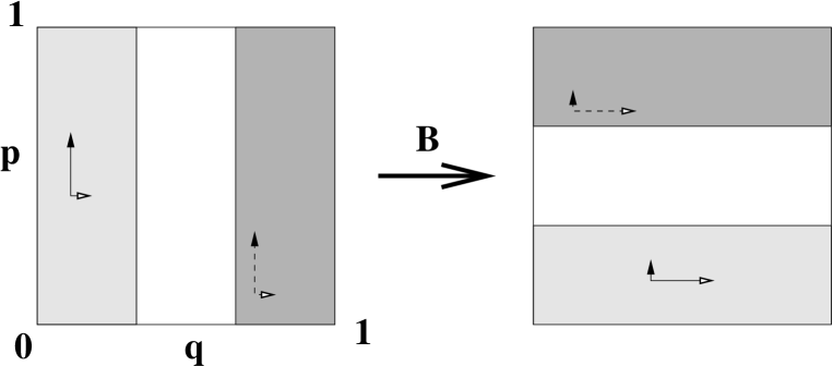
Figure 2.1. Schematic representation of the baker’s map (2.1) for $D=3$. The arrows show the vertical contraction and horizontal dilation.

The map preserves the symplectic form $dp\wedge dq$. It is uniformly hyperbolic, with constant Liapounov exponent $\lambda=\log D$. The stable (resp. unstable) directions are the vertical (resp. horizontal) directions.

2.2. Symbolic dynamics

The map $B$ can be easily expressed in terms of the $D$-nary representation of the coordinates $(q,p)$. Indeed, let us represent the position $q\in[0,1)$ and momentum $p\in[0,1)$ of any point $x=(q,p)\in{\mathbb{T}}^{2}$ through their $D$-nary sequences

$$q=0.\epsilon_{1}\epsilon_{2}\ldots,\qquad p=0.\epsilon^{\prime}_{1}\epsilon^{\prime}_{2}\ldots\,,\quad\text{where the ``symbols''}\quad\epsilon_{i},\,\epsilon^{\prime}_{i}\in\left\{0,\ldots,D-1\right\}\equiv\mathbb{Z}_{D}\,.$$

We then associate with $x=(q,p)$ the following bi-infinite sequence

$$x\equiv\ldots\epsilon^{\prime}_{2}\epsilon^{\prime}_{1}\,\cdot\,\epsilon_{1}\epsilon_{2}\ldots.$$

Symbolic sequences will be shortly denoted by $\boldsymbol{\epsilon}=\epsilon_{1}\epsilon_{2}\ldots$, without precising their lengths (either finite or infinite), and from there $x\equiv\boldsymbol{\epsilon}^{\prime}\cdot\boldsymbol{\epsilon}$.

More formally, we call $\Sigma_{+}=\left\{0,\ldots,D-1\right\}^{\mathbb{N}_{*}}$ the set of one-sided infinite sequences, and $\Sigma=\Sigma_{+}\times\Sigma_{+}$, the set of two-sided infinite sequences. The $D$-nary decomposition then generates a map

$$J:\Sigma \longrightarrow[0,1)\times[0,1)$$

$$\boldsymbol{\epsilon}^{\prime}\cdot\boldsymbol{\epsilon} \longmapsto x=(0.\boldsymbol{\epsilon},\,0.\boldsymbol{\epsilon}^{\prime})\,.$$

The map $J$ is one-to-one except on a denumerable set where it is two-to-one (for instance, $\ldots 00\cdot 100\ldots$ is sent to the same point as $\ldots 11\cdot 011\ldots$). Let us equip $\Sigma$ with the distance

(2.2) $$d_{\Sigma}(\boldsymbol{\epsilon}^{\prime}\cdot\boldsymbol{\epsilon},\,\boldsymbol{\alpha}^{\prime}\cdot\boldsymbol{\alpha})=\max(D^{-n_{0}^{\prime}},\,D^{-n_{0}})\,,$$

where $n_{0}=\min\left\{n\geq 0\,:\,\epsilon_{n+1}\neq\alpha_{n+1}\right\}$ and similarly for $n_{0}^{\prime}$. The map $J$ is Lipschitz-continuous with respect to this distance.

$J$ gives a semiconjugacy between, on one side, the action of $B$ on the torus, on the other side, the simple shift on $\Sigma$:

(2.3) $$B\big{(}J(\boldsymbol{\epsilon}^{\prime}\cdot\boldsymbol{\epsilon})\big{)}=J(\ldots\epsilon^{\prime}_{2}\epsilon^{\prime}_{1}\epsilon_{1}\,\cdot\,\epsilon_{2}\epsilon_{3}\ldots)\,.$$

This is a very simple example of symbolic coding of a dynamical system. The action of $B$ on $\Sigma$ is Lipschitz-continuous, as opposed to its discontinuous action on ${\mathbb{T}}^{2}$ equipped with its standard topology. As long as we are only interested in characterizing the entropies of invariant measures, it is harmless to identify the two systems. In the following discussion we will go back and forth between the two representations.

2.3. Topological and metric entropies

Let $(X,d)$ be a compact metric space, and $T:X\to X$ a continuous map. In this section, we give the definitions and some properties of the topological and metric entropies associated with the map $T$ on $X$. We then consider the particular case of the map $B$, seen as the shift acting on $\Sigma$.

2.3.1. Topological entropy

The topological entropy of the dynamical system $(X,T)$ is defined as follows: for any $n>0$, define the distance

$$d_{n}^{T}(x,y)\stackrel{{\scriptstyle\rm{def}}}{{=}}\max_{m=0,...,n}d(T^{m}x,T^{m}y)\,.$$

For any $r>0$, let $N_{T}(r,n)$ be the minimal cardinal of a covering of $X$ by balls of radius $r$ for the distance $d_{n}^{T}$. Then the topological entropy of the set $X$ with respect to the map $T$ is defined as

$$h_{top}(X,T)\stackrel{{\scriptstyle\rm def}}{{=}}\lim_{r\to 0}\limsup_{n\to\infty}\frac{1}{n}\log N_{T}(r,n)\,.$$

In many cases, it is not necessary to let $r\to 0$: there exists $r_{0}>0$ such that, for any $0<r\leq r_{0}$, the topological entropy is equal to $\limsup_{n\to\infty}\frac{1}{n}\log N_{T}(r,n)$.

In the case $X=\Sigma$ (equipped with the metrics $d_{\Sigma}$ given in (2.2)), the topological entropy can be expressed using cylinder sets. Given two sequences $\boldsymbol{\epsilon}$, $\boldsymbol{\epsilon}^{\prime}$ of finite lengths $|\boldsymbol{\epsilon}|=n$, $|\boldsymbol{\epsilon}^{\prime}|=n^{\prime}$, we define the cylinder set $[\boldsymbol{\epsilon}^{\prime}\cdot\boldsymbol{\epsilon}]\subset\Sigma$ as the set of sequences starting with $\boldsymbol{\epsilon}$ on the right side and with $\boldsymbol{\epsilon}^{\prime}$ on the left side. If $n=n^{\prime}$, it is a ball of radius $D^{-n}$ for the distance $d_{\Sigma}$. The image of $[\boldsymbol{\epsilon}^{\prime}\cdot\boldsymbol{\epsilon}]$ on the torus is the rectangle

$$J([\boldsymbol{\epsilon}^{\prime}\cdot\boldsymbol{\epsilon}])=[\frac{j}{D^{n}},\frac{j+1}{D^{n}}]\times[\frac{j^{\prime}}{D^{n^{\prime}}},\frac{j^{\prime}+1}{D^{n^{\prime}}}]\,,\quad\text{where}\quad\frac{j}{D^{n}}=0.\epsilon_{1}\cdots\epsilon_{n},\ \frac{j^{\prime}}{D^{n^{\prime}}}=0.\epsilon^{\prime}_{1}\cdots\epsilon^{\prime}_{n^{\prime}}\,.$$

In the following we will often identify cylinders and rectangles.

Since we are interested in the action of the shift, we can focus our attention to one-sided cylinder sets, of the form $[\cdot\boldsymbol{\epsilon}]$, corresponding on the torus to “vertical” rectangles $[\frac{j}{D^{n}},\frac{j+1}{D^{n}}]\times[0,1]$. The set of cylinders $[\cdot\boldsymbol{\epsilon}]$ of length $n=|\boldsymbol{\epsilon}|$ will be called $\Sigma_{n}$.

Let now $F$ be a closed subset of $\Sigma$, invariant under the action of $B$. Call $N_{B}(n,F)$ the minimal number of cylinder sets $[\cdot\boldsymbol{\epsilon}]$ of length $n$ necessary to cover $F$. The topological entropy $h_{top}(F,B)$, also denoted by $h_{top}(F)$, is then given by

(2.4) $$h_{top}(F)=\limsup_{n\to\infty}\frac{1}{n}\log N_{B}(n,F)\,.$$

Examples. If $F=\mathcal{O}$ is a periodic orbit, we find $h_{top}(\mathcal{O})=0$. If $F={\mathbb{T}}^{2}$, we find $h_{top}({\mathbb{T}}^{2})=\log D$. It is also useful to note that, if $F$ and $G$ are two closed invariant subsets, then $h_{top}(F\cup G)=\max(h_{top}(F),h_{top}(G)).$

2.3.2. Metric entropy

Going back to the general framework, we consider a $T$-invariant probability measure $\mu$ on the metric space $X$.

If $\mathcal{P}=(P_{1},...,P_{n})$ is a finite measurable partition of $X$ (meaning that $X$ is the disjoint union of the $P_{i}$s), we define the entropy of the measure $\mu$ with respect to the partition $\mathcal{P}$ by

(2.5) $$h_{\mathcal{P}}(\mu)=-\sum_{i}\mu(P_{i})\log\mu(P_{i})\,.$$

For $\mathcal{P}=(P_{1},...,P_{n})$ and $\mathcal{Q}=(Q_{1},...,Q_{m})$ any two partitions of $X$, we can define a new partition $\mathcal{P}\vee\mathcal{Q}$ as the partition composed of the sets $P_{i}\cap Q_{j}$. The entropy has the following subadditivity property:

(2.6) $$h_{\mathcal{P}\vee\mathcal{Q}}(\mu)\leq h_{\mathcal{P}}(\mu)+h_{\mathcal{Q}}(\mu)\,.$$

We may now use the map $T$ to refine a given partition $\mathcal{P}$: for any $n\geq 1$ we define the partition

$$\mathcal{P}^{(n)}=\mathcal{P}\vee T^{-1}\mathcal{P}\vee...\vee T^{-(n-1)}\mathcal{P}\,.$$

By the subadditivity property, they satisfy

$$h_{\mathcal{P}^{(n+m)}}(\mu)\leq h_{\mathcal{P}^{(n)}}(\mu)+h_{T^{-n}\mathcal{P}^{(m)}}(\mu)\,.$$

If the measure $\mu$ is $T$-invariant, $h_{T^{-n}\mathcal{P}^{(m)}}(\mu)=h_{\mathcal{P}^{(m)}}(\mu)$. The subadditivity of the sequence $\big{(}h_{\mathcal{P}^{(n)}}(\mu)\big{)}_{n\geq 1}$ implies the existence of the limit:

(2.7) $$\lim_{n\to\infty}\frac{1}{n}\,h_{\mathcal{P}^{(n)}}(\mu)=\inf_{n\geq 1}\frac{1}{n}\,h_{\mathcal{P}^{(n)}}(\mu)\stackrel{{\scriptstyle\rm{def}}}{{=}}h_{\mathcal{P}}(\mu,T)\,.$$

This number $h_{\mathcal{P}}(\mu,T)$ is the entropy of the measure $\mu$ for the action of $T$, with respect to the partition $\mathcal{P}$. The Kolmogorov-Sinai entropy of the triplet $(X,T,\mu)$, denoted by $h_{KS}(\mu,T)$, is the supremum of $h_{\mathcal{P}}(\mu,T)$ over all finite measurable partitions $\mathcal{P}$.

2.3.3. Generating partition for the baker’s map

In the case we will be interested in, namely the shift $B$ acting on $\Sigma$, this supremum is reached if we start from the partition $\mathcal{P}$ made of the cylinder sets of length one, that is of the form $[.\epsilon_{1}]$ for $\epsilon_{1}\in\mathbb{Z}_{D}$. Each such cylinder is mapped on the torus into a vertical rectangles $[\frac{\epsilon_{1}}{D},\frac{\epsilon_{1}+1}{D}]\times[0,1)$. Obviously, the refined partition $\mathcal{P}^{(n)}$ is made of the cylinder sets $[.\boldsymbol{\epsilon}]$ of length $n$, representing vertical rectangles $[\frac{j}{D^{n}},\frac{j+1}{D^{n}}]\times[0,1)$. For any $B$-invariant measure $\mu$ on ${\mathbb{T}}^{2}$, the metric entropy $h_{KS}(\mu,B)=h_{KS}(\mu)$ is given by

(2.8) $$h_{KS}(\mu)=\inf_{n\geq 1}\frac{1}{n}\,h_{\mathcal{P}^{(n)}}(\mu)=\lim_{n\to\infty}\frac{1}{n}\,h_{\mathcal{P}^{(n)}}(\mu)\,.$$

Examples. If $\mu=\delta_{\mathcal{O}}$ is an invariant measure carried on a periodic orbit, we find $h_{KS}(\delta_{\mathcal{O}})=0$. Another class of interesting examples are Bernoulli measures : given some probability weights $p_{0},...,p_{D-1}$ ($p_{\epsilon}\geq 0$, $\sum_{\epsilon}p_{\epsilon}=1$), the infinite product measure $\mu_{Ber}=\big{(}\sum_{\epsilon=0}^{D-1}p_{\epsilon}\delta_{\epsilon}\big{)}^{\otimes\mathbb{Z}}$ on $\Sigma$ is invariant under the shift. On ${\mathbb{T}}^{2}$, it gives a $B$-invariant probability measure, with simple self-similarity properties. Its Kolmogorov-Sinai entropy is $h_{KS}(\mu_{Ber})=-\sum_{\epsilon}p_{\epsilon}\log p_{\epsilon}$. The Lebesgue measure corresponds to the case $p_{\epsilon}\equiv D^{-1}$ and has maximal entropy, $h_{KS}(\mu_{Leb})=\log D$. It is also useful to know that the functional $h_{KS}$ is affine on the convex set of invariant probability measures.

Let us now describe the quantum framework we will be working with.

3. Walsh quantization of the baker’s map

3.1. Weyl quantization of the 2-torus

The usual way to “quantize” the torus phase space ${\mathbb{T}}^{2}$ consists in periodizing quantum states $\psi\in\mathcal{S}^{\prime}(\mathbb{R})$ in both position and momentum; the resulting vector space $\mathcal{H}_{N}$ is nontrivial if and only if Planck’s constant $\hbar=(2\pi N)^{-1}$, $N\in\mathbb{N}$, in which case it has dimension $N$. An orthonormal basis of $\mathcal{H}_{N}$ is given by the “position eigenstates” $\left\{\boldsymbol{q}_{j},\;j=0,\ldots,N-1\right\}$ localized at positions $q_{j}=j/N$. The “momentum eigenstates” are obtained from the latter by applying the inverse of the Discrete Fourier Transform $\mathcal{F}_{N}$,

(3.1) $$(\mathcal{F}_{N})_{jk}=\frac{1}{\sqrt{N}}\,e^{-2i\pi kj/N}\,,\quad j,k=0,\ldots,N-1\,.$$

This Fourier transform was the basic ingredient used by Balazs and Voros to quantize the baker’s map [2, 34]. Precisely, in the case where $N$ is a multiple of $D$, the (Weyl) quantum baker is defined as the following unitary matrix in the position basis:

(3.2) $$B_{N}^{BV}=\mathcal{F}_{N}^{-1}\begin{pmatrix}\mathcal{F}_{N/D}&0&0\\ 0&\ddots&0\\ 0&0&\mathcal{F}_{N/D}\end{pmatrix}$$

These matrices have been studied in detail [35], but little rigorous is known about their spectrum. They suffer from diffraction effects due to the classical discontinuities of $B$ (the Egorov property is slightly problematic, but still allows one to prove Quantum Ergodicity [9]). It was recently observed [29] that some eigenstates of the 2-baker in the case $N=2^{k}$, ($k\in\mathbb{N}$) have an interesting multifractal structure in phase space. These eigenstates were analyzed using the Walsh-Hadamard transform.

3.2. Walsh quantum kinematics

In the present work, we will use the Walsh transform as a building block to quantize the baker’s map. As we will see, the resulting Walsh quantization of $B$ respects its $D$-nary coding, and allows for an exact spectral analysis. It has already been used in [31] in the case of “open” baker’s maps.

Before quantizing the map $B$ itself, we must first describe the Walsh quantum setting on the 2-dimensional torus, obtained by replacing the usual Fourier transform by the Walsh-Fourier transform. The latter was originally defined in the framework of signal processing [24]. More recently, it has been used as a toy model in several problems of harmonic analysis (see e.g. the introduction to the “Walsh phase space” in [38]).

3.2.1. Walsh transform

We will use a Walsh transform adapted to the $D$-baker (2.1). The values of Planck’s constant we will be considering are of the form $\left\{\hbar=\hbar_{k}=(2\pi D^{k})^{-1},\ k\in\mathbb{N}\right\}$, so the semiclassical limit reads $k\to\infty$. The quantum Hilbert space is then isomorphic to $\mathbb{C}^{D}\otimes\cdots\otimes\mathbb{C}^{D}$ (with $k$ factors). More precisely, if we call $\left\{e_{0},\ldots,e_{D-1}\right\}$ an orthonormal basis of $\mathbb{C}^{D}$, and identify each index $j\in\left\{0,\ldots,D^{k}-1\right\}$ with its $D$-nary expansion $j\equiv\epsilon_{1}\cdots\epsilon_{k}$, then the isomorphism $\mathcal{H}_{D^{k}}\simeq(\mathbb{C}^{D})^{\otimes k}$ is realized through the orthonormal basis of position eigenstates:

(3.3) $$\boldsymbol{q}_{j}=e_{\epsilon_{1}}\otimes e_{\epsilon_{2}}\otimes\cdots\otimes e_{\epsilon_{k}}\,.$$

Each factor space $\mathbb{C}^{D}$ is called a “quantum $D$it”, or qu$D$it, in the quantum computing framework. We see that each qu$D$it is associated with a particular position scale.

The Walsh transform on $\mathcal{H}_{D^{k}}$, which we denote by $W_{D^{k}}$, is a simplification of the Fourier transform $\mathcal{F}_{D^{k}}$. It can be defined in terms of the $D$-dimensional Fourier transform $\mathcal{F}_{D}$ (see (3.1)) through its action on tensor product states

(3.4) $$W_{D^{k}}(v^{(1)}\otimes\ldots\otimes v^{(k)})=\mathcal{F}_{D}v^{(k)}\otimes\mathcal{F}_{D}v^{(k-1)}\otimes\ldots\otimes\mathcal{F}_{D}v^{(1)},\qquad v^{(i)}\in\mathbb{C}^{D},\ i=1,\ldots,k\,.$$

The image of position eigenstates through $W_{D^{k}}^{*}$ yields the orthonormal basis of momentum eigenstates. To each momentum $p_{l}=l/D^{k}=0.\epsilon^{\prime}_{1}\ldots\epsilon^{\prime}_{k}$, $l=0,\ldots,D^{k}-1$ is associated the state

$$\boldsymbol{p}_{l}=\sum_{j=0}^{D^{k}-1}\big{(}W_{D^{k}}^{*}\big{)}_{lj}\boldsymbol{q}_{j}=\mathcal{F}_{D}^{*}e_{\epsilon^{\prime}_{k}}\otimes\mathcal{F}_{D}^{*}e_{\epsilon^{\prime}_{k-1}}\otimes\cdots\otimes\mathcal{F}_{D}^{*}e_{\epsilon^{\prime}_{1}}\,.$$

Therefore, each qu$D$it also corresponds to a particular momentum scale (in reverse order with respect to its corresponding position scale).

From now on, we will often omit the subscript $D$ on the Fourier transform, and simply write $\mathcal{F}=\mathcal{F}_{D}$.

3.2.2. Quantum rectangles and Walsh coherent states

Given any integer $0\leq\ell\leq k$, two sequences $\boldsymbol{\epsilon}=\epsilon_{1}\ldots\epsilon_{\ell}\in\Sigma_{\ell}$, $\boldsymbol{\epsilon}^{\prime}=\epsilon^{\prime}_{1}\ldots\epsilon^{\prime}_{k-\ell}\in\Sigma_{k-\ell}$ define a rectangle $[\boldsymbol{\epsilon}^{\prime}\cdot\boldsymbol{\epsilon}]$ of area $\Delta q\Delta p=D^{-k}=h_{k}$: for this reason, we call it a quantum rectangle (in the time-frequency framework [38], such rectangles are called tiles). To this rectangle we associate the Walsh coherent state $|\boldsymbol{\epsilon}^{\prime}\cdot\boldsymbol{\epsilon}^{\prime}\rangle$ defined as follows:

(3.5) $$|\boldsymbol{\epsilon}^{\prime}\cdot\boldsymbol{\epsilon}\rangle\stackrel{{\scriptstyle\rm{def}}}{{=}}e_{\epsilon_{1}}\otimes e_{\epsilon_{2}}\otimes\ldots e_{\epsilon_{\ell}}\otimes\mathcal{F}^{*}e_{\epsilon^{\prime}_{k-\ell}}\otimes\ldots\otimes\mathcal{F}^{*}e_{\epsilon^{\prime}_{1}}\,.$$

For each choice of $\ell$, $0\leq\ell\leq k$, we consider the family of quantum rectangles

(3.6) $$\mathcal{R}^{k,\ell}\stackrel{{\scriptstyle\rm def}}{{=}}\left\{[\boldsymbol{\epsilon}^{\prime}\cdot\boldsymbol{\epsilon}]\ :\ \boldsymbol{\epsilon}\in\Sigma_{\ell},\ \boldsymbol{\epsilon}^{\prime}\in\Sigma_{k-\ell}\right\}\,.$$

The corresponding family of coherent states $\left\{|\boldsymbol{\epsilon}^{\prime}\cdot\boldsymbol{\epsilon}\rangle\,:\,[\boldsymbol{\epsilon}^{\prime}\cdot\boldsymbol{\epsilon}]\in\mathcal{R}^{k,\ell}\right\}$ then forms an orthonormal basis of $\mathcal{H}_{D^{k}}$, which we will call the $\ell$-basis, or basis of $\ell$-coherent states. The state $|\boldsymbol{\epsilon}^{\prime}\cdot\boldsymbol{\epsilon}\rangle$ is strictly localized in the corresponding rectangle $[\boldsymbol{\epsilon}^{\prime}\cdot\boldsymbol{\epsilon}]$, in the following sense:

$$\forall j\equiv\alpha_{1}\ldots\alpha_{k},\quad\begin{cases}|\langle\boldsymbol{q}_{j}|\boldsymbol{\epsilon}^{\prime}\cdot\boldsymbol{\epsilon}\rangle|&=D^{-\ell/2}\qquad\text{if}\ \alpha_{1}=\epsilon_{1},\ldots,\alpha_{\ell}=\epsilon_{\ell},\qquad 0\ \text{otherwise}\\ |\langle\boldsymbol{p}_{j}|\boldsymbol{\epsilon}^{\prime}\cdot\boldsymbol{\epsilon}\rangle|&=D^{-(k-\ell)/2}\quad\text{if}\ \alpha_{1}=\epsilon^{\prime}_{1},\ldots,\alpha_{k-\ell}=\epsilon^{\prime}_{k-\ell},\qquad 0\ \text{otherwise}\,.\end{cases}$$

This property of strict localization in both position and momentum is the main reason why Walsh harmonic analysis is easier to manipulate than the usual Fourier analysis (where such a localization is impossible). Obviously, for $\ell=k$ (resp. $\ell=0$) we recover the position (resp. momentum) eigenbasis.

Each $\ell$-basis provides a Walsh-Husimi representation of $\psi\in\mathcal{H}_{D^{k}}$: it is the non-negative function $WH^{k,\ell}_{\psi}$ on ${\mathbb{T}}^{2}$, constant inside each rectangle $[\boldsymbol{\epsilon}^{\prime}\cdot\boldsymbol{\epsilon}]\in\mathcal{R}^{k,\ell}$, where it takes the value:

(3.7) $$WH^{k,\ell}_{\psi}(x)\stackrel{{\scriptstyle\rm def}}{{=}}D^{k}\,\left|\langle\psi|\boldsymbol{\epsilon}^{\prime}\cdot\boldsymbol{\epsilon}\rangle\right|^{2},\qquad x\in[\boldsymbol{\epsilon}^{\prime}\cdot\boldsymbol{\epsilon}]\,.$$

The standard (“Gaussian”) Husimi function of a state $\psi$ contains all the information about that state (apart from a nonphysical phase prefactor) [21]. On the opposite, the Walsh-Husimi function $WH^{k,\ell}_{\psi}$ only contains “half” the information on $\psi$ (namely, the moduli of the components of $\psi$ in the $\ell$-basis). This important difference will not bother us in the following.

In the case of a tensor-product state $\psi=v^{(1)}\otimes v^{(2)}\otimes\cdots\otimes v^{(k)}$ (each $v^{(i)}\in\mathbb{C}^{D}$) relevant in Section 4.2, we have :

$$WH^{k,\ell}_{\psi}(x)=D^{k}\big{|}v_{\epsilon_{1}}^{(1)}\big{|}^{2}\ldots\big{|}v_{\epsilon_{\ell}}^{(\ell)}\big{|}^{2}\>\big{|}(\mathcal{F}v^{(k)})_{\epsilon^{\prime}_{1}}\big{|}^{2}\ldots\big{|}(\mathcal{F}v^{(\ell+1)})_{\epsilon^{\prime}_{k-\ell}}\big{|}^{2}\,,\qquad x\in[\boldsymbol{\epsilon}^{\prime}\cdot\boldsymbol{\epsilon}]\,.$$

If $\psi$ is normalized, $WH^{k,\ell}_{\psi}$ defines a probability density on the torus (or on $\Sigma$). For any measurable subset $A\subset{\mathbb{T}}^{2}$, we will denote its measure by

$$WH^{k,\ell}_{\psi}(A)=\int_{A}WH^{k,\ell}_{\psi}(x)\,dx\,.$$

In the semiclassical limit, a sequence of coherent states $\left\{|\boldsymbol{\epsilon}^{\prime}\cdot\boldsymbol{\epsilon}\rangle\right\}$ can be associated with a single phase space point $x\in{\mathbb{T}}^{2}$ only if both sidelengths $D^{-\ell}$, $D^{k-\ell}$ of the associated rectangles decrease to zero. This is the case if and only if the index $\ell=\ell(k)$ is chosen to depend on $k$, in the following manner:

(3.8) $$\ell(k)\to\infty\quad\text{and}\quad k-\ell(k)\to\infty\quad\text{as}\quad k\to\infty\,.$$

Therefore, to define semiclassical limit measures of sequences of eigenstates $\big{(}\psi_{k}\in\mathcal{H}_{D^{k}}\big{)}_{k\to\infty}$, we will consider sequences of Husimi representations $\big{(}WH^{k,\ell}\big{)}$ satisfying the above conditions. For instance, we can consider the “symmetric” choice $\ell=\lfloor k/2\rfloor$.

3.2.3. Anti-Wick quantization of observables

In standard quantum mechanics, coherent states may also be used to quantize observables (smooth functions on ${\mathbb{T}}^{2}$), using the anti-Wick procedure. In the Walsh framework, a similar (Walsh-)anti-Wick quantization can be defined, but now it rather makes sense on observables $f$ on ${\mathbb{T}}^{2}\simeq\Sigma$ which are Lipschitz-continuous with respect to the distance (2.2), denoted by $f\in Lip(\Sigma)$. The reason to choose this functional space (instead of some space of smooth functions on ${\mathbb{T}}^{2}$) is that we want to prove Egorov’s theorem, which involves both $f$ and its iterate $f\circ B$. It is therefore convenient to require that both these functions belong to the same space (we could also consider Hölder-continuous functions on $\Sigma$).

The Walsh-anti-Wick quantization is defined as follows. For any $k$, one selects a family of quantum rectangles (3.6), such that $\ell=\ell(k)$ satisfies the semiclassical condition (3.8). The quantization of the observable $f$ is the following operator on $\mathcal{H}_{D^{k}}$:

(3.9) $$\operatorname{Op}_{k,\ell}(f)\stackrel{{\scriptstyle\rm def}}{{=}}D^{k}\sum_{[\boldsymbol{\epsilon}^{\prime}\cdot\boldsymbol{\epsilon}]\in\mathcal{R}^{k,\ell}}|\boldsymbol{\epsilon}^{\prime}\cdot\boldsymbol{\epsilon}\rangle\langle\boldsymbol{\epsilon}^{\prime}\cdot\boldsymbol{\epsilon}|\;\int_{[\boldsymbol{\epsilon}^{\prime}\cdot\boldsymbol{\epsilon}]}f(x)\,dx=\sum_{[\boldsymbol{\epsilon}^{\prime}\cdot\boldsymbol{\epsilon}]\in\mathcal{R}^{k,\ell}}|\boldsymbol{\epsilon}^{\prime}\cdot\boldsymbol{\epsilon}\rangle\langle\boldsymbol{\epsilon}^{\prime}\cdot\boldsymbol{\epsilon}|\;\overline{f}^{[\boldsymbol{\epsilon}^{\prime}\cdot\boldsymbol{\epsilon}]}\,.$$

Here and in the following, we denote by $\overline{f}^{R}$ the average of $f$ over the rectangle $R$. For each $\ell$, the above operators form a commutative algebra, namely the algebra of diagonal matrices in the $\ell$-basis. The quantization $\operatorname{Op}_{k,\ell}$ is in some sense the dual of the Husimi representation $WH^{k,\ell}$ :

(3.10) $$\forall f\in Lip(\Sigma),\ \forall\psi\in\mathcal{H}_{D^{k}},\qquad\langle\psi|\operatorname{Op}_{k,\ell}(f)|\psi\rangle=\int_{{\mathbb{T}}^{2}}WH^{k,\ell}_{\psi}(x)\,f(x)\,dx\,.$$

The following proposition shows that this family of quantizations satisfy a certain number of “reasonable” properties. We recall that the Lipschitz norm of $f\in Lip(\Sigma)$ is defined as

$$\|f\|_{Lip}\stackrel{{\scriptstyle\rm{def}}}{{=}}\sup_{x\in\Sigma}|f(x)|+\sup_{x\neq y\in\Sigma}\frac{|f(x)-f(y)|}{d_{\Sigma}(x,y)}\,.$$

Proposition 3.1.

i) For any index $0\leq\ell\leq k$ and observable $f\in Lip(\Sigma)$, one has

$$\operatorname{Op}_{k,\ell}(f^{*})=\operatorname{Op}_{k,\ell}(f)^{*},\qquad{\rm tr}\big{(}\operatorname{Op}_{k,\ell}(f)\big{)}=D^{k}\,\int_{{\mathbb{T}}^{2}}f(x)\,dx\,.$$

ii) For any $0\leq\ell\leq k$ and observables $f,g\in Lip(\Sigma)$,

(3.11) $$\|\operatorname{Op}_{k,\ell}(f\,g)-\operatorname{Op}_{k,\ell}(f)\operatorname{Op}_{k,\ell}(g)\|\leq\|f\|_{Lip}\,\|g\|_{Lip}\,D^{-\min(\ell,k-\ell)}\,.$$

iii) For any pair of indices $0\leq\ell^{\prime}\leq\ell\leq k$, the two quantizations $\operatorname{Op}_{k,\ell}$, $\operatorname{Op}_{k,\ell^{\prime}}$ are related as follows:

$$\forall f\in Lip(\Sigma),\qquad\|\operatorname{Op}_{k,\ell}(f)-\operatorname{Op}_{k,\ell^{\prime}}(f)\|\leq 2\,\|f\|_{Lip}\,D^{-\min(\ell^{\prime},k-\ell)}\,.$$

The first two statements make up the “correspondence principle for quantum observables” of Marklof and O’Keefe [27, Axiom 2.1], which they use to prove Quantum Ergodicity (see Theorem 3.4 below).

The third statement implies that if $\ell^{\prime}\leq\ell$ (depending on $k$) both satisfy the semiclassical condition (3.8), then the two quantizations are asymptotically equivalent.

Proof.

The statement $i)$ is obvious from the definition (3.9) and the fact that $\ell$-coherent states form an orthonormal basis.

To prove $ii)$ and $iii)$ we use the Lipschitz regularity of the observables. The variations of $f\in Lip(\Sigma)$ inside a rectangle $R=[\boldsymbol{\alpha}^{\prime}\cdot\boldsymbol{\alpha}]$ are bounded as follows:

$$\forall x,y\in R,\qquad|f(x)-f(y)|\leq\|f\|_{Lip}\,d_{\Sigma}(x,y)\leq\|f\|_{Lip}\,\operatorname{diam}(R)\,,$$

where the diameter of the rectangle $R$ for the metrics $d_{\Sigma}$ is $\operatorname{diam}(R)=D^{-\min(|\boldsymbol{\alpha}|,|\boldsymbol{\alpha}^{\prime}|)}$. As a consequence,

(3.12) $$\forall x\in R,\qquad\left|f(x)-\overline{f}^{R}\right|\leq\|f\|_{Lip}\,\operatorname{diam}(R)\,.$$

To show $ii)$, we expand the operator in the left hand side of (3.11):

$$\operatorname{Op}_{k,\ell}(f\,g)-\operatorname{Op}_{k,\ell}(f)\operatorname{Op}_{k,\ell}(g)=\sum_{[\boldsymbol{\epsilon}^{\prime}\cdot\boldsymbol{\epsilon}]\in\mathcal{R}^{k,\ell}}|\boldsymbol{\epsilon}^{\prime}\cdot\boldsymbol{\epsilon}\rangle\langle\boldsymbol{\epsilon}^{\prime}\cdot\boldsymbol{\epsilon}|\;\left(\overline{(fg)}^{[\boldsymbol{\epsilon}^{\prime}\cdot\boldsymbol{\epsilon}]}-\overline{f}^{[\boldsymbol{\epsilon}^{\prime}\cdot\boldsymbol{\epsilon}]}\;\overline{g}^{[\boldsymbol{\epsilon}^{\prime}\cdot\boldsymbol{\epsilon}]}\right)\,.$$

Using (3.12) for $R=[\boldsymbol{\epsilon}^{\prime}\cdot\boldsymbol{\epsilon}]\in\mathcal{R}^{k,\ell}$, we easily bound the terms on the right hand side:

$$\forall[\boldsymbol{\epsilon}^{\prime}\cdot\boldsymbol{\epsilon}]\in\mathcal{R}^{k,\ell}\,,\qquad\left|\overline{(fg)}^{[\boldsymbol{\epsilon}^{\prime}\cdot\boldsymbol{\epsilon}]}-\overline{f}^{[\boldsymbol{\epsilon}^{\prime}\cdot\boldsymbol{\epsilon}]}\;\overline{g}^{[\boldsymbol{\epsilon}^{\prime}\cdot\boldsymbol{\epsilon}]}\right|\leq\|f\|_{Lip}\,\|g\|_{Lip}\,D^{-\min(\ell,k-\ell)}\,.$$

Since the $\ell$-coherent states are orthogonal, Pythagore’s theorem gives the bound (3.11).

To prove the statement $iii)$, we need to consider “mesoscopic rectangles” of the type $R=[\boldsymbol{\alpha}^{\prime}\cdot\boldsymbol{\alpha}]$ where $|\boldsymbol{\alpha}|=\ell^{\prime}$, $|\boldsymbol{\alpha}^{\prime}|=k-\ell$. Such a rectangle $R$ supports $D^{\ell-\ell^{\prime}}$ quantum rectangles of type $\mathcal{R}^{k,\ell}$, and the same number of rectangles of type $\mathcal{R}^{k,\ell^{\prime}}$. We want to analyze the partial difference

(3.13) $$\Delta\operatorname{Op}(f)_{|R}\stackrel{{\scriptstyle\rm def}}{{=}}\sum_{\begin{subarray}{l}[\boldsymbol{\epsilon}^{\prime}\cdot\boldsymbol{\epsilon}]\in\mathcal{R}^{k,\ell}\\ [\boldsymbol{\epsilon}^{\prime}\cdot\boldsymbol{\epsilon}]\subset R\end{subarray}}|\boldsymbol{\epsilon}^{\prime}\cdot\boldsymbol{\epsilon}\rangle\langle\boldsymbol{\epsilon}^{\prime}\cdot\boldsymbol{\epsilon}|\;\overline{f}^{[\boldsymbol{\epsilon}^{\prime}\cdot\boldsymbol{\epsilon}]}-\sum_{\begin{subarray}{l}[\boldsymbol{\epsilon}^{\prime}\cdot\boldsymbol{\epsilon}]\in\mathcal{R}^{k,\ell^{\prime}}\\ [\boldsymbol{\epsilon}^{\prime}\cdot\boldsymbol{\epsilon}]\subset R\end{subarray}}|\boldsymbol{\epsilon}^{\prime}\cdot\boldsymbol{\epsilon}\rangle\langle\boldsymbol{\epsilon}^{\prime}\cdot\boldsymbol{\epsilon}|\;\overline{f}^{[\boldsymbol{\epsilon}^{\prime}\cdot\boldsymbol{\epsilon}]}\,.$$

Both terms of the difference act inside the same subspace

$$V_{R}=\operatorname{span}\left\{|\boldsymbol{\epsilon}^{\prime}\cdot\boldsymbol{\epsilon}\rangle\,:\,[\boldsymbol{\epsilon}^{\prime}\cdot\boldsymbol{\epsilon}]\in\mathcal{R}^{k,\ell},[\boldsymbol{\epsilon}^{\prime}\cdot\boldsymbol{\epsilon}]\subset R\right\}.$$

We then use (3.12) to show that the average of $f$ over any quantum rectangle $[\boldsymbol{\epsilon}^{\prime}\cdot\boldsymbol{\epsilon}]\subset R$ satisfies

$$\left|\overline{f}^{[\boldsymbol{\epsilon}^{\prime}\cdot\boldsymbol{\epsilon}]}-\overline{f}^{R}\right|\leq\|f\|_{Lip}\,\operatorname{diam}(R)\,.$$

Inserted in (3.13), this estimate yields the upper bound:

$$\|\Delta\operatorname{Op}(f)_{|R}\|\leq 2\,\|f\|_{Lip}\,\operatorname{diam}(R)\,.$$

Finally, since the subspaces $V_{R}$, $V_{R}^{\prime}$ associated with two disjoint rectangles $R\neq R^{\prime}$ are orthogonal, Pythagore’s theorem implies the statement $iii)$. ∎

3.3. Walsh-quantized baker

We are now in position to adapt the Balazs-Voros quantization of the $D$-baker’s map (2.1) to the Walsh framework, by mimicking (3.2). We define the Walsh quantization of $B$ by the following unitary matrix $B_{k}$ in the position basis:

(3.14) $$B_{k}\stackrel{{\scriptstyle\rm def}}{{=}}W_{D^{k}}^{-1}\begin{pmatrix}W_{D^{k-1}}&0&0\\ 0&\ddots&0\\ 0&0&W_{D^{k-1}}\end{pmatrix}\,.$$

This operator acts simply on tensor product states:

(3.15) $$B_{k}(v^{(1)}\otimes\ldots\otimes v^{(k)})=v^{(2)}\otimes v^{(3)}\otimes\ldots\otimes v^{(k)}\otimes\mathcal{F}_{D}^{*}v^{(1)}\,.$$

Similarly, a tensor-product operator on $\mathcal{H}_{D^{k}}$ will be transformed as follows by the quantum baker:

(3.16) $$B_{k}(A^{(1)}\otimes\ldots\otimes A^{(k)})B_{k}^{-1}=A^{(2)}\otimes A^{(3)}\otimes\ldots\otimes A^{(k)}\otimes\mathcal{F}_{D}^{*}A^{(1)}\mathcal{F}_{D}\,.$$

These formulas are clearly reminiscent of the shift (2.3) produced by the classical map. The main difference lies in the fact that “quantum sequences” are of finite length $k$, the shift acting cyclically on the sequence, and one needs to act with $\mathcal{F}^{*}_{D}$ on the last qu$D$it.

This quantization of the baker’s map has been introduced before, as the extreme member among a family of different quantizations [36], and some of its semiclassical properties have been studied in [39]. In particular, it was shown that, within the standard Wigner-Weyl formalism, this family of quantum propagators does not quantize the baker’s map, but a multivalued version of it.

On the other hand, in this paper we will stick to the Walsh-anti-Wick formalism to quantize observables, and in this setting we prove in the next proposition that the quantum baker (3.14) quantizes the original baker’s map.

Proposition 3.2 (Egorov theorem).

Let us select a quantization $\operatorname{Op}_{k,\ell}$ satisfying the semiclassical conditions (3.8). Then, for any observable $f\in Lip(\Sigma)$, we have in the semiclassical limit

$$\|B_{k}^{-1}\operatorname{Op}_{k,\ell}(f)B_{k}-\operatorname{Op}_{k,\ell}(f\circ B)\|\leq 2\,\|f\|_{Lip}\,D^{1-\min(\ell,k-\ell-1)}\,.$$

For the “symmetric” choice $\ell=\lfloor k/2\rfloor$, the right hand side is of order $D^{-k/2}\sim\hbar^{1/2}$.

Proof.

The crucial argument is the fact that, for any index $0<\ell\leq k$, the Walsh-baker maps $\ell$-coherent states onto $(\ell-1)$-coherent states. This fact is obvious from the definition (3.5) and the action of $B_{k}$ on tensor product states (3.15):

(3.17) $$\forall[\boldsymbol{\epsilon}^{\prime}\cdot\boldsymbol{\epsilon}]\in\mathcal{R}^{k,\ell},\qquad B_{k}|\boldsymbol{\epsilon}^{\prime}\cdot\boldsymbol{\epsilon}\rangle=|B(\boldsymbol{\epsilon}^{\prime}\cdot\boldsymbol{\epsilon})\rangle=|\epsilon^{\prime}_{k-\ell}\ldots\epsilon^{\prime}_{2}\epsilon^{\prime}_{1}\epsilon_{1}\,\cdot\,\epsilon_{2}\ldots\epsilon_{\ell}\rangle\,.$$

Notice that the shifted rectangle $B([\boldsymbol{\epsilon}^{\prime}\cdot\boldsymbol{\epsilon}])\in\mathcal{R}^{k,\ell-1}$. As a result, the evolved operator $B_{k}^{-1}\operatorname{Op}_{k,\ell}(f)B_{k}$ will be a sum of terms of the form

$$|B^{-1}(\boldsymbol{\epsilon}^{\prime}\cdot\boldsymbol{\epsilon})\rangle\langle B^{-1}(\boldsymbol{\epsilon}^{\prime}\cdot\boldsymbol{\epsilon})|\;\overline{f}^{[\boldsymbol{\epsilon}^{\prime}\cdot\boldsymbol{\epsilon}]}=|B^{-1}(\boldsymbol{\epsilon}^{\prime}\cdot\boldsymbol{\epsilon})\rangle\langle B^{-1}(\boldsymbol{\epsilon}^{\prime}\cdot\boldsymbol{\epsilon})|\;\overline{f}^{B^{-1}([\boldsymbol{\epsilon}^{\prime}\cdot\boldsymbol{\epsilon}])}\;,$$

which implies the exact formula

(3.18) $$B_{k}^{-1}\operatorname{Op}_{k,\ell}(f)B_{k}=\operatorname{Op}_{k,\ell+1}(f\circ B)\,.$$

The third statement of Proposition 3.1 and the inequality $\|f\circ B\|_{Lip}\leq D\,\|f\|_{Lip}$ yield the estimate. ∎

Remark 1.

The exact evolution (3.17) is similar with the evolution of Gaussian coherent states through quantum cat maps [11]. It is also the Walsh counterpart of the coherent state evolution through the Weyl-quantized baker $B^{BV}_{N}$, used in [9] to prove a weak version of Egorov’s property. In that case, the coherent states needed to be situated “far away” from the discontinuities of $B$, which implied that Egorov’s property only held for observables vanishing in some neighbourhood of the discontinuities. In the present framework, we do not need to take care of discontinuities, since $B$ is continuous in the topology of $\Sigma$.

Remark 2.

The integer $k$ satisfies $k=\frac{|\log h|}{\log D}$, where $h=h_{k}=D^{-k}$ is Planck’s constant, and $\log D$ the uniform Liapounov exponent of the classical baker’s map: $k$ is the Ehrenfest time for the quantum baker. As in the Weyl formalism [9], the Egorov property can be extended to iterates $(B_{k})^{n}$ up to times $n\approx(1-\delta)\frac{k}{2}$, for any fixed $\delta>0$.

The exact evolution of coherent states (3.17) also implies the following property, dual of Eq. (3.18):

$$\forall\psi\in\mathcal{H}_{D^{k}},\qquad WH^{k,\ell}_{B_{k}\psi}=WH^{k,\ell-1}_{\psi}\circ B^{-1}\,.$$

In particular, if $\psi$ is an eigenstate of $B_{k}$, one has

$$WH^{k,\ell}_{\psi}=WH^{k,\ell-1}_{\psi}\circ B^{-1}\,,$$

meaning that the classical map sends one Husimi representation to the next one.

The Egorov estimate of Proposition 3.2 leads to the following

Corollary 3.3 (Invariance of semiclassical measures).

Consider a semiclassical sequence $(\psi_{k}\in\mathcal{H}_{D^{k}})_{k\in\mathbb{N}_{*}}$ such that each $\psi_{k}$ is an eigenstate of $B_{k}$. It induces a sequence of Husimi measures $\big{(}WH^{k,\ell}_{\psi_{k}}\big{)}$, where $\ell=\ell(k)$ is assumed to satisfy (3.8). Up to extracting a subsequence, one can assume that this sequence converges to a probability measure $\mu$ on $\Sigma$.

Then the measure $\mu$ is invariant through the baker’s map $B$.

This measure $\mu$ projects to a measure on ${\mathbb{T}}^{2}$, which we will also (with a slight abuse) call $\mu$. The proof of Quantum Ergodicity [7, 45], starting from the ergodicity of the classical map with respect to the Lebesgue measure, is also valid within our nonstandard quantization. Indeed, as shown in [27], the statements $i),ii)$ of Proposition 3.1 and the Egorov theorem (Prop. 3.2) suffice to prove Quantum Ergodicity for the Walsh-quantized baker:

Theorem 3.4 (Quantum Ergodicity).

For any $k\in\mathbb{N}_{*}$, select an orthonormal eigenbasis $(\psi_{k,j}\in\mathcal{H}_{D^{k}})_{j=0,\ldots,D^{k}-1}$ of the Walsh-quantized baker $B_{k}$.

Then, for any $k\geq 1$, there exists a subset $J_{k}\subset\left\{0,\ldots,D^{k}-1\right\}$ such that

• $\lim_{k\to\infty}\frac{\sharp J_{k}}{D^{k}}=1$ (“almost all eigenstates”)

• if $\ell(k)$ satisfies (3.8) and $j(k)\in J_{k}$ for all $k\geq 1$, then the sequence of Husimi measures $(WH^{k,\ell(k)}_{\psi_{k,j(k)}})$ weakly converges to the Lebesgue measure on ${\mathbb{T}}^{2}$.

Remark 3.

In the following section we will be working with partitions into the vertical rectangles $[\cdot\boldsymbol{\alpha}]$, $|\boldsymbol{\alpha}|=n$, which make up the partition $\mathcal{P}^{(n)}$ (see section 2.3.3). For any state $\psi\in\mathcal{H}_{D^{k}}$, the measure $WH^{k,k}_{\psi}$ assigns the weight $|\langle\boldsymbol{q}_{j}|\psi\rangle|^{2}$ to each vertical quantum rectangle $[\cdot\boldsymbol{\epsilon}]$, $|\boldsymbol{\epsilon}|=k$. With respect to the partition $\mathcal{P}^{(n)}$, all Husimi measures $WH^{k,\ell}_{\psi}$, $n\leq\ell\leq k$ are equivalent: for any cylinder $[\cdot\boldsymbol{\alpha}]\in\mathcal{P}^{(n)}$, we indeed have

(3.19) $$\forall\ell,\ n\leq\ell\leq k,\qquad WH^{k,\ell}_{\psi}([\cdot\boldsymbol{\alpha}])=WH^{k,k}_{\psi}([\cdot\boldsymbol{\alpha}])\,.$$

4. Some explicit eigenstates of $B_{k}$

The interest of the quantization $B_{k}$ lies in the fact that its spectrum and eigenstates can be analytically computed.

4.1. Short quantum period

The crucial point (derived from the identity (3.15) and the periodicity of the Fourier transform) is that this operator is periodic, with period $2k$ (when $D=2$) or $4k$ (when $D\geq 3$):

$$D=2 \Longrightarrow\forall k\geq 1,\quad(B_{k})^{2k}=I_{2^{k}}$$

$$D\geq 2 \Longrightarrow\forall k\geq 1,\quad(B_{k})^{4k}=I_{D^{k}}\,.$$

More precisely, $(B_{k})^{2k}$ is the involution

(4.1) $$(B_{k})^{2k}=\Pi\otimes\Pi\cdots\otimes\Pi\,,$$

where $\Pi$ is the “parity operator” on $\mathbb{C}^{D}$, which sends $e_{\epsilon}$ to $e_{\bar{\epsilon}}$, with $\epsilon+\bar{\epsilon}\equiv 0\bmod D$.

As we noticed above, $k=\frac{|\log h|}{\log D}$ is the Ehrenfest time of the system, so the above periodicity can be compared with the “short quantum periods” of the quantum cat map [5, 11], which allowed one to construct eigenstates with a partial localization on some periodic orbits. The first consequence of this logarithmic period is the very high degeneracy of the eigenvalues $\left\{e^{2i\pi r/4k},\ \ r=0,\ldots,4k-1\right\}$: each of them is approximately $\frac{D^{k}}{4k}$-degenerate. In the case of the cat map, this huge degeneracy gives sufficient freedom to construct eigenstates which are partially scarred on a periodic orbit [11]. In the Walsh-baker case, although $4k$ is the double of what was called a “short period” in [11], $(B_{k})^{2k}$ sends a coherent state $|\boldsymbol{\epsilon}^{\prime}\cdot\boldsymbol{\epsilon}\rangle$ to another coherent state $|\bar{\boldsymbol{\epsilon}}^{\prime}\cdot\bar{\boldsymbol{\epsilon}}\rangle$, and we are still able to construct half-scarred eigenstates. Due to (4.1), a state scarred on the periodic orbit indexed by the periodic sequence $(\epsilon_{1}\epsilon_{2}\ldots\epsilon_{p})$ is also scarred, with the same weight, on the “mirror” orbit $(\bar{\epsilon}_{1}\bar{\epsilon}_{2}\ldots\bar{\epsilon}_{p})$.

Figure 4.1. Eigenstates of $B_{k}$ for $D=2$. The grey scale corresponds to a logarithmic representation of $WH^{k,\ell}_{\psi}(x)$ (black=large; white=small). Top left: eigenstate half-scarred at the origin, $k=10$, $\ell=5$. Top right: tensor product eigenstate (4.2), $k=11$, $\ell=6$. Bottom: eigenstate (4.6) with a fractal support, $k=11$, $\ell=6$ (white=zero).

4.2. Tensor-product eigenstates

A new feature, compared with the quantum cat map, is that we straightforwardly obtain eigenstates of $B_{k}$ which are not “scarred” on any periodic orbit, but still have a nontrivial phase space distribution: the associated semiclassical measure is a singular Bernoulli measure. These states are constructed as follows: take any eigenstate $w\in\mathbb{C}^{D}$ of the inverse Fourier transform $\mathcal{F}_{D}^{*}$. Then, for any $k\geq 1$, the tensor-product state

(4.2) $$\psi=w\otimes\cdots\otimes w\in\mathcal{H}_{D^{k}}$$

is an eigenstate of $B_{k}$. From (3.7), its Husimi measure $WH^{k,\ell}_{\psi}$ has the following weight on a quantum rectangle $[\boldsymbol{\epsilon}^{\prime}\cdot\boldsymbol{\epsilon}]\in\mathcal{R}^{k,\ell}$:

(4.3) $$WH^{k,\ell}_{\psi}([\boldsymbol{\epsilon}^{\prime}\cdot\boldsymbol{\epsilon}])=|w_{\epsilon_{1}}|^{2}\ldots|w_{\epsilon_{\ell}}|^{2}\>|w_{\epsilon^{\prime}_{1}}|^{2}\ldots|w_{\epsilon^{\prime}_{k-\ell}}|^{2}\,.$$

This shows that $WH^{k,\ell}_{\psi}$ is the product of a measure $\nu_{\ell}$ on the horizontal interval by a measure $\nu_{k-\ell}$ on the vertical interval. $\nu_{\ell}$ (resp. $\nu_{k-\ell}$) can be obtained by conditioning a certain self-similar measure $\nu$ on subintervals of type $[\frac{j}{D^{\ell}},\frac{j+1}{D^{\ell}})$ (resp. $[\frac{j}{D^{k-\ell}},\frac{j+1}{D^{k-\ell}})$). This measure $\nu$ is constructed by iteration: the first step consists in splitting $[0,1)$ into $D$ subintervals $[\frac{\epsilon}{D},\frac{\epsilon+1}{D})$, and allocating the weight $p_{\epsilon}=|w_{\epsilon}|^{2}$ to the $\epsilon$-th subinterval. The next step splits each subinterval, etc. In other words, for any finite sequence $\boldsymbol{\epsilon}\in\Sigma_{n}$, the measure of the interval $[\cdot\boldsymbol{\epsilon}]$ is given by

$$\nu([\cdot\boldsymbol{\epsilon}])=p_{\epsilon_{1}}p_{\epsilon_{2}}\ldots p_{\epsilon_{n}}\,.$$

In the symbolic representation $[0,1)\sim\Sigma_{+}$, $\nu$ is a Bernoulli measure.

The Husimi measure $WH^{k,\ell}_{\psi}$ is therefore the measure

$$\mu=\nu(dq)\times\nu(dp),\quad\text{conditioned on the rectangles }[\boldsymbol{\epsilon}^{\prime}\cdot\boldsymbol{\epsilon}]\in\mathcal{R}^{k,\ell}\,.$$

Assuming that $\ell$ satisfies the condition (3.8) (so that the diameters of the rectangles vanish as $k\to\infty$), we get

$$\lim_{k\to\infty}WH^{k,\ell}_{\psi}=\mu\,,$$

where the limit should be understood in the weak sense.

The measure $\mu$ is obviously a Bernoulli invariant measure, of the type shown in the Examples of Section 2.3.3. Let us describe some particular cases, forgetting for a moment that the state $w$ is an eigenstate of $\mathcal{F}^{*}_{D}$, and taking for $w$ any normalized state in $\mathbb{C}^{D}$.

• if the coefficients $p_{\epsilon}$ are all equal, $p_{\epsilon}=1/D$, then $\mu=dx$ is the Lebesgue measure.

• if there is a single $\epsilon\in\left\{0,\ldots,D-1\right\}$ such that $p_{\epsilon}=1$ and the others vanish, then $\mu=\delta_{x_{o}}$, where $x_{o}\equiv\ldots\epsilon\epsilon\,\cdot\,\epsilon\epsilon\epsilon\ldots$ is a fixed point of $B$. Obviously, this is impossible if $w$ an eigenstate of $\mathcal{F}^{*}_{D}$.

• in the remaining cases, $\mu$ is a purely singular continuous measure on ${\mathbb{T}}^{2}$, with simple self-similarity properties.

Topological entropy of tensor product eigenstates

An eigenstate $w$ of $\mathcal{F}^{*}_{D}$ can have a certain number of vanishing coefficients. Call $S\subset\left\{0,\ldots,D-1\right\}$ the set of non-vanishing coefficients, and $d=\sharp S$ its cardinal. If $d<D$, the corresponding measure $\mu$ is then supported on a proper invariant subset $F_{\mu}$ of ${\mathbb{T}}^{2}$, corresponding to the sequences $\boldsymbol{\epsilon}^{\prime}\cdot\boldsymbol{\epsilon}\in\Sigma$ with all coefficients $\epsilon_{i},\epsilon^{\prime}_{i}\in S$. One can easily check that the topological entropy of $F_{\mu}$ is given by

$$h_{top}(F_{\mu})=\log(d)\,.$$

Now, because all the matrix elements of $\mathcal{F}^{*}_{D}$ are of modulus $D^{-1/2}$, the number $d$ of non-vanishing components of $w$ is bounded as

(4.4) $$d\geq\sqrt{D}\,,\qquad\mbox{so that}\quad h_{top}(F_{\mu})\geq\frac{\log D}{2}\,.$$

This proves that semiclassical measures $\mu$ obtained from sequences of tensor-product eigenstates (4.2) satisfy the general lower bound of Theorem 1.1.

The simplest example of such eigenstates seems to be for $D=4$: $\mathcal{F}_{4}^{*}$ admits the eigenstate $w=(1,0,1,0)/\sqrt{2}$. The corresponding limit measure $\mu$ is supported on a subset $F_{\mu}$ which saturates the lower bound (4.4): $h_{top}(F_{\mu})=\log 2=\frac{\log 4}{2}$.

Metric entropy of tensor product eigenstates

For a normalized state $w\in\mathbb{C}^{D}$, the Kolmogorov-Sinai entropy of the measure $\mu$ can be shown to be

$$h_{KS}(\mu)=-\sum_{\epsilon=0}^{D-1}p_{\epsilon}\log p_{\epsilon}=-\sum_{\epsilon=0}^{D-1}|w_{\epsilon}|^{2}\log|w_{\epsilon}|^{2}\stackrel{{\scriptstyle\rm{def}}}{{=}}h(w).$$

A priori, this function could take any value between $0$ and $\log D$, the topological entropy of ${\mathbb{T}}^{2}$ with respect to the baker’s map. However, as in the case of the topological entropy, imposing $w$ to be an eigenstate of $\mathcal{F}^{*}_{D}$ restricts the possible range of $h(w)$. Indeed, the following “Entropic Uncertainty Principle”, first conjectured by Kraus [19] and proven in [26], direcly provides the desired lower bound for $h(w)$.

Theorem 4.1 (Entropic Uncertainty Principle [26]).

For any $M\in\mathbb{N}_{*}$, let $U$ be a unitary $M\times M$ matrix and $c(U)\stackrel{{\scriptstyle\rm def}}{{=}}\sup_{i,j}|U_{ij}|$. Then, for any normalized state $\psi\in\mathbb{C}^{M}$, one has

$$h(\psi)+h(U\psi)\geq-2\log c(U)\,,$$

where the entropy is defined as $h(\psi)=-\sum_{i}|\psi_{i}|^{2}\log|\psi_{i}|^{2}$.

The proof of this theorem (which is the major ingredient in the proof of Theorem 1.2, see Section 5) is outlined in the Appendix.

Applying this theorem to the matrix $U=\mathcal{F}_{D}^{*}$, and using the fact that $w$ is an eigenstate of that matrix, we obtain the desired lower bound

(4.5) $$h_{KS}(\mu)=h(w)\geq\frac{\log D}{2}.$$

The above example of tensor-product eigenstates of the $4$-baker, constructed from $w=(1,0,1,0)/\sqrt{2}$, also saturate this inequality: $h_{KS}(\mu)=h_{top}(F_{\mu})=\frac{\log 4}{2}$.

4.3. A slightly more complicated example

In the case of $D=2$, although none of the eigenvectors of $F_{2}$ has any vanishing component, one can still construct eigenstates converging to a fractal measure supported on a proper subset of ${\mathbb{T}}^{2}$. Indeed, we notice that $\mathcal{F}_{2}\,e_{0}=\frac{e_{0}+e_{1}}{\sqrt{2}}\stackrel{{\scriptstyle\rm def}}{{=}}e_{+}$, and $\mathcal{F}_{2}^{2}=I_{2}$. As a result, in the case $k$ is odd, the state

(4.6) $$\psi=\frac{1}{\sqrt{2}}\left(e_{0}\otimes e_{+}\otimes e_{0}\otimes\ldots e_{+}\otimes e_{0}+e_{+}\otimes e_{0}\otimes e_{+}\otimes\ldots e_{0}\otimes e_{+}\right)$$

is an eigenstate of $B_{k}$. It becomes normalized in the limit $k\to\infty$, and one can check that the associated semiclassical measure is $\mu=\frac{1}{2}\left(\nu_{1}(dq)\times\nu_{2}(dp)+\nu_{2}(dq)\times\nu_{1}(dp)\right)$, where $\nu_{1}$ (resp. $\nu_{2}$) is the self-similar measures on $[0,1)$ obtained by splitting $[0,1)$ in $4$ equal subintervals, which are allocated the weights $(1/2,1/2,0,0)$ (resp. $(1/2,0,1/2,0)$), and so on. One can easily show that this semiclassical measure $\mu$ saturates both lower bounds: $h_{KS}(\mu)=h_{top}(F_{\mu})=\frac{\log 2}{2}$.

5. Proof of Theorem 1.2: Lower bound on the metric entropy

Applying Theorem 4.1 in a more clever way, we can generalize the lower bound (4.5) to any semiclassical measure $\mu$, thereby proving Theorem 1.2. In this section we give ourselves a sequence $\big{(}\psi_{k}\in\mathcal{H}_{D^{k}}\big{)}$ of eigenstates of $B_{k}$, and assume that the associated Husimi measures converge to an invariant probability measure $\mu$.

5.1. Quantum partition of unity

The definition of metric entropy given in Section 2.3.2 starts from the “coarse” partition $\mathcal{P}$ (made of $D$ rectangles $[\cdot\epsilon]$), which is then refined into a sequence of partitions $\mathcal{P}^{(n)}$ using the classical dynamics. A natural way to study the Kolmogorov-Sinai entropy of quantum eigenstates is to transpose these objects to the quantum framework. For any anti-Wick quantization $\operatorname{Op}_{k,\ell}$ satisfying the condition (3.8), the characteristic functions ${\mathchoice{1\mskip-4.0mu{\rm{l}}}{1\mskip-4.0mu{\rm{l}}}{1\mskip-4.5mu{\rm{l}}}{1\mskip-5.0mu{\rm{l}}}}_{[\cdot\epsilon]}$ are quantized into the orthogonal projectors

(5.1) $$P_{\epsilon}=\pi_{\epsilon}\otimes(I)^{\otimes k-1}\,,\qquad\epsilon=0,\ldots,D-1\,.$$

Here, $\pi_{\epsilon}$ is the orthogonal projector on the basis state $e_{\epsilon}\in\mathbb{C}^{D}$, and $I=I_{D}$ is the identity operator on $\mathbb{C}^{D}$. This family of projectors make up a “quantum partition of unity”:

$$\sum_{\epsilon=0}^{D-1}P_{\epsilon}=(I)^{\otimes k}=I_{D^{k}}\,.$$

Like its classical counterpart, this partition can be refined using the dynamics. To an evolved rectangle $B^{-l}([\cdot\epsilon])$ corresponds the projector

$$P_{\epsilon}(l)\stackrel{{\scriptstyle\rm def}}{{=}}B_{k}^{-l}\,P_{\epsilon}\,B_{k}^{l}\,.$$

From there, the quantum counterpart of the refined partition $\mathcal{P}^{(n)}=\left\{[\cdot\boldsymbol{\epsilon}],\>\,\boldsymbol{\epsilon}\in\Sigma_{n}\right\}$ is composed of the following operators:

(5.2) $$P_{\boldsymbol{\epsilon}}\stackrel{{\scriptstyle\rm def}}{{=}}P_{\epsilon_{n}}(n-1)\circ\ldots\circ P_{\epsilon_{2}}(1)\circ P_{\epsilon_{1}}\,.$$

Using the formula (3.16), we find that

(5.3) $$n\leq k\Longrightarrow P_{\boldsymbol{\epsilon}}=\pi_{\epsilon_{1}}\otimes\pi_{\epsilon_{2}}\otimes\ldots\pi_{\epsilon_{n}}\otimes(I)^{\otimes k-n}\,.$$

This shows that $P_{\boldsymbol{\epsilon}}$ is an orthogonal projector associated with the rectangle $[\cdot\boldsymbol{\epsilon}]$. It is equal to $\operatorname{Op}_{k,\ell}({\mathchoice{1\mskip-4.0mu{\rm{l}}}{1\mskip-4.0mu{\rm{l}}}{1\mskip-4.5mu{\rm{l}}}{1\mskip-5.0mu{\rm{l}}}}_{[\cdot\boldsymbol{\epsilon}]})$ if $n\leq\ell$. In the extreme case $n=k$, these operators project on single position eigenstates:

$$\forall j=\epsilon_{1}\ldots\epsilon_{k}\in\left\{0,\ldots,D^{k}-1\right\},\qquad P_{\boldsymbol{\epsilon}}=|\boldsymbol{q}_{j}\rangle\langle\boldsymbol{q}_{j}|\,.$$

Using Remark 3, we see that these projectors can be direcly used to express the weight of the Husimi measures on rectangles. Indeed, if $n\leq\ell\leq k$ and $[\cdot\boldsymbol{\epsilon}]\in\Sigma_{n}$, then

(5.4) $$WH^{k,\ell}_{\psi_{k}}([\cdot\boldsymbol{\epsilon}])=\|P_{\boldsymbol{\epsilon}}\,\psi_{k}\|^{2}\,.$$

From there, we straightforwardly deduce the:

Lemma 5.1.

Provided $n\leq\ell\leq k$, the entropy (2.5) of the Husimi measure $WH^{k,\ell}_{\psi_{k}}$, relative to the refined partition $\mathcal{P}^{(n)}$, can be written as follows:

(5.5) $$h_{\mathcal{P}^{(n)}}(WH^{k,\ell}_{\psi_{k}})=-\sum_{|\boldsymbol{\epsilon}|=n}\|P_{\boldsymbol{\epsilon}}\,\psi_{k}\|^{2}\,\log\big{(}\|P_{\boldsymbol{\epsilon}}\,\psi_{k}\|^{2}\big{)}\,.$$

For some values of the indices, this quantity corresponds to well-known “quantum entropies”.

5.2. Shannon and Wehrl entropies

By setting $n=\ell=k$ in the above Lemma, we obtain a “quantum” entropy which has been used before to characterize the localization properties of individual states [16]. It is simply the Shannon entropy of the state $\psi\in\mathcal{H}_{N}$, when expressed in the position basis $\left\{\boldsymbol{q}_{j},\;j=0,\ldots,N-1\right\}$:

(5.6) $$h_{Shannon}(\psi)\stackrel{{\scriptstyle\rm{def}}}{{=}}h_{\mathcal{P}^{(k)}}(WH^{k,k}_{\psi})=-\sum_{j=0}^{N-1}|\langle\boldsymbol{q}_{j}|\psi\rangle|^{2}\,\log\big{(}|\langle\boldsymbol{q}_{j}|\psi\rangle|^{2}\big{)}\,.$$

This entropy obviously selects a preferred “direction” in phase space: one could as well consider the Shannon entropy in the momentum basis. To avoid this type of choice, it has become more fashionable to use a quantum entropy based on the Husimi representation of quantum states, introduced by Wehrl [41]. In the Weyl framework, it is given by the integral over the phase space of $\eta(|\langle x|\psi\rangle|^{2})$, where $\eta(s)=-s\log s$, and $\left\{|x\rangle\,:\,x\in{\mathbb{T}}^{2}\right\}$ is a continuous family of Gaussian coherent states.

In the Walsh framework, the coherent states form discrete families, so the integral is effectively a sum. For any index $\ell$, we define the Walsh-Wehrl entropy of $\psi\in\mathcal{H}_{D^{k}}$ as:

(5.7) $$h^{k,\ell}_{Wehrl}(\psi)=-\sum_{[\boldsymbol{\epsilon}^{\prime}\cdot\boldsymbol{\epsilon}]\in\mathcal{R}^{k,\ell}}|\langle\boldsymbol{\epsilon}^{\prime}\cdot\boldsymbol{\epsilon}|\psi\rangle|^{2}\,\log\big{(}|\langle\boldsymbol{\epsilon}^{\prime}\cdot\boldsymbol{\epsilon}|\psi\rangle|^{2}\big{)}\,.$$

Notice that the Shannon entropy (5.6) is a particular case of the Wehrl entropy, obtained by setting $\ell=k$. Eq. (3.17) implies that all quantum entropies of eigenstates are equal:

Proposition 5.2.

If $\psi_{k}\in\mathcal{H}_{D^{k}}$ is an eigenstate of the Walsh-baker $B_{k}$, then its Wehrl and Shannon entropies are all equal:

$$\forall\ell\in[0,k],\qquad h^{k,\ell}_{Wehrl}(\psi_{k})=h_{Shannon}(\psi_{k})\,.$$

As in the case of Gaussian coherent states [41, 23], localized states have a small Wehrl entropy: the minimum of $h^{k,\ell}_{Wehrl}(\psi)$ is reached for $\psi=|\boldsymbol{\epsilon}^{\prime}\cdot\boldsymbol{\epsilon}\rangle$ a coherent state in the $\ell$-basis, where the entropy vanishes. On the opposite, the entropy is maximal when $\psi$ is equidistributed with respect to the $\ell$-basis, and the entropy then takes the value $\log N=|\log 2\pi\hbar|$. Notice that the extremal properties of the entropy $h^{k,\ell}_{Wehrl}$ of pure quantum states are much easier to analyze than those of the “Gaussian” Wehrl entropies on the plane, the torus or the sphere [23, 22, 30].

The Shannon or Wehrl entropies can be now bounded from below using the Entropic Uncertainty Principle, Theorem 4.1. Indeed, $\psi_{k}$ is an eigenstate of the iterate $(B_{k})^{k}$, which is the tensor product operator

(5.8) $$(B_{k})^{k}=\mathcal{F}_{D}^{*}\otimes\mathcal{F}_{D}^{*}\otimes\ldots\otimes\mathcal{F}_{D}^{*}\,.$$

The matrix elements of this operator in the position basis are all of modulus $D^{-k/2}$. Thus, Theorem 4.1 implies that

(5.9) $$h_{Shannon}(\psi_{k})=h_{\mathcal{P}^{(k)}}(WH^{k,k}_{\psi_{k}})\geq\frac{k}{2}\log D\,.$$

Using the property that the Wehrl entropies (5.7) of an eigenstate are all equal to each other (see Proposition 5.2), this proves Theorem 1.4.

In the expression for the Shannon entropy, both the Husimi measure $WH^{k,\ell}_{\psi_{k}}$ and the partition $\mathcal{P}^{(n)}$ depend on the semiclassical parameter $k$ in a rigid way, namely $\ell=n=k$. On the other hand, if we want to understand the entropy of the semiclassical measure $\mu$, we should first estimate the entropy of some $k$-independent partition $\mathcal{P}^{(n)}$, then take the semiclassical limit ($k\to\infty$) of the Husimi measures $WH^{k,\ell}_{\psi_{k}}$ with the condition (3.8) satisfied, and only send $n$ to infinity afterwards. In other words, we need to control the entropies (5.5) for a fixed $n\in\mathbb{N}$ while sending $k,\ell\to\infty$.

In the following sections, we present two different approaches to realize this program, both yielding a proof of Theorem 1.2.

5.3. First method: use of subadditivity

The first approach consists in estimating the entropy (5.5) of the partition $\mathcal{P}^{(n)}$ for some fixed $n$, starting from the lower bound (5.9) on the entropy of $\mathcal{P}^{(k)}$. Both these entropies are taken on the measure $\mu_{k}\stackrel{{\scriptstyle\rm{def}}}{{=}}WH^{k,k}_{\psi_{k}}$. This estimation uses the subadditivity property (2.6).

Using Euclidean division, we can write $k=qn+r$ with $q,r\in\mathbb{N}$, $r<n$. The subadditivity of entropy implies that

(5.10) $$h_{\mathcal{P}^{(k)}}(\mu_{k})\leq h_{\mathcal{P}^{(n)}}(\mu_{k})+h_{B^{-n}\mathcal{P}^{(n)}}(\mu_{k})+\ldots+h_{B^{-(q-1)n}\mathcal{P}^{(n)}}(\mu_{k})+h_{B^{-qn}\mathcal{P}^{(r)}}(\mu_{k}).$$

The very last term, being the entropy of a partition of $D^{r}$ elements, is less than $r\log D$.

Using the fact that $\psi_{k}$ is an eigenstate of $B_{k}$, we prove below that the Husimi measure $\mu_{k}$ is invariant under $B$ until the Ehrenfest time :

Lemma 5.3.

For any $n$-rectangle $[\cdot\boldsymbol{\epsilon}]$ of the partition $\mathcal{P}^{(n)}$, for any index $0\leq l\leq k-n$, we have

$$\mu_{k}(B^{-l}[\cdot\boldsymbol{\epsilon}])=\mu_{k}([\cdot\boldsymbol{\epsilon}])\,.$$

This straighforwardly implies the following property:

$$l\leq k-n\Longrightarrow h_{B^{-l}\mathcal{P}^{(n)}}(\mu_{k})=h_{\mathcal{P}^{(n)}}(\mu_{k})\,.$$

Injecting this equality in the subadditivity (5.10), and using the lower bound (5.9) for $h_{\mathcal{P}^{(k)}}(\mu_{k})$, we obtain a lower bound for the entropy of the fixed partition $\mathcal{P}^{(n)}$:

(5.11) $$h_{\mathcal{P}^{(n)}}(\mu_{k})\geq\frac{1}{q}\Big{(}h_{\mathcal{P}^{(k)}}(\mu_{k})-r\log D\Big{)}\geq\frac{1}{q}\Big{(}k\frac{\log D}{2}-r\log D\Big{)}\,.$$

From the identity (3.19), and assuming that $\lfloor k/2\rfloor>n$, the left hand side is also the entropy of the Husimi measure $WH^{k,\lfloor k/2\rfloor}_{\psi_{k}}$, which converges to $\mu$ in the semiclassical limit. On the right hand side, $k/q\to n$ and $r/q\to 0$ as $k\to\infty$, so in the limit,

$$h_{\mathcal{P}^{(n)}}(\mu)\geq\frac{n}{2}\,\log D\,.$$

We can finally let $n\to\infty$, and get Theorem 1.2.∎

Proof of Lemma 5.3

For any $n$-rectangle $[\cdot\boldsymbol{\epsilon}]$ of the partition $\mathcal{P}^{(n)}$, we have

$$\mu_{k}([\cdot\boldsymbol{\epsilon}]) =\left\|\pi_{\epsilon_{1}}\otimes\ldots\pi_{\epsilon_{n}}\otimes(I)^{\otimes k-n}\psi_{k}\right\|^{2}$$

$$=\left\|(B_{k})^{-l}\,\big{(}\pi_{\epsilon_{1}}\otimes\ldots\pi_{\epsilon_{n}}\otimes(I)^{\otimes k-n}\big{)}\,(B_{k})^{l}\psi_{k}\right\|^{2},$$

where we have used the facts that $\psi_{k}$ is an eigenfunction of $B_{k}$, and that $B_{k}$ is unitary. Now, using (3.16), the last line can be transformed into

$$\left\|(I)^{\otimes l}\otimes\pi_{\epsilon_{1}}\otimes\ldots\pi_{\epsilon_{n}}\otimes(I)^{\otimes k-n-l}\,\psi_{k}\right\|^{2} =\sum_{\alpha_{1},\ldots,\alpha_{l}=0}^{D-1}\left\|\pi_{\alpha_{1}}\otimes\ldots\pi_{\alpha_{l}}\otimes\pi_{\epsilon_{1}}\otimes\ldots\pi_{\epsilon_{n}}\otimes(I)^{\otimes k-n-l}\,\psi_{k}\right\|^{2}$$

$$=\sum_{\alpha_{1},\ldots,\alpha_{l}}\left\|P_{\boldsymbol{\alpha}\boldsymbol{\epsilon}}\psi_{k}\right\|^{2} =\sum_{\boldsymbol{\alpha}=(\alpha_{1},\ldots,\alpha_{l})}\mu_{k}([\cdot\boldsymbol{\alpha}\boldsymbol{\epsilon}])=\mu_{k}(B^{-l}[\cdot\boldsymbol{\epsilon}])\,.$$

The last equality is due to the fact that the set $B^{-l}[\cdot\boldsymbol{\epsilon}]$ is the disjoint union

(5.12) $$B^{-l}[\cdot\boldsymbol{\epsilon}]=\bigcup_{\alpha_{1},\ldots,\alpha_{l}=0}^{D-1}[\cdot\boldsymbol{\alpha}\boldsymbol{\epsilon}]\,.$$

∎

5.4. Second method: vectorial Entropic Uncertainty Principle

The second approach to bound (5.5) from below is to directly apply to that sum the vectorial version of the Entropic Uncertainty Principle, given in Theorem A.3 in the Appendix.

Indeed, for any $n\leq k$, the family of orthogonal projectors $\left\{P_{\boldsymbol{\epsilon}},\;|\boldsymbol{\epsilon}|=n\right\}$ satisfy $P_{\boldsymbol{\epsilon}}P_{\boldsymbol{\epsilon}^{\prime}}=\delta_{\boldsymbol{\epsilon}\boldsymbol{\epsilon}^{\prime}}P_{\boldsymbol{\epsilon}}$, and the resolution of unity

$$\sum_{|\boldsymbol{\epsilon}|=n}P_{\boldsymbol{\epsilon}}=I\,.$$

Any state $\psi\in{\mathcal{H}}_{D^{k}}$ can be decomposed into the sequence of states $\left\{\psi_{\boldsymbol{\epsilon}}=P_{\boldsymbol{\epsilon}}\psi,\;|\boldsymbol{\epsilon}|=n\right\}$, in terms of which the entropy (5.5) can then be written as

(5.13) $$h_{\mathcal{P}^{(n)}}(\mu_{k})=-\sum_{|\boldsymbol{\epsilon}|=n}\|\psi_{\boldsymbol{\epsilon}}\|^{2}\;\log\|\psi_{\boldsymbol{\epsilon}}\|^{2}\stackrel{{\scriptstyle\rm def}}{{=}}h_{n}(\psi)\,.$$

The vectorial Entropic Uncertainty Principle (Theorem A.3), specialized to this family of orthogonal projectors, reads as follows :

Theorem 5.4.

For a given $n\leq k$, and any normalized state $\psi\in{\mathcal{H}}_{D^{k}}$, let us define the entropy

$$h_{n}(\psi)=-\sum_{|\boldsymbol{\epsilon}|=n}\|\psi_{\boldsymbol{\epsilon}}\|^{2}\;\log\|\psi_{\boldsymbol{\epsilon}}\|^{2}\,.$$

Let $U$ be a unitary operator on $\mathcal{H}_{D^{k}}$. For any sequences $\boldsymbol{\epsilon}$, $\boldsymbol{\epsilon}^{\prime}$ of length $n$, we call $U_{\boldsymbol{\epsilon},\boldsymbol{\epsilon}^{\prime}}=P_{\boldsymbol{\epsilon}}UP_{\boldsymbol{\epsilon}^{\prime}}$, and $c_{n}(U)=\sup_{|\boldsymbol{\epsilon}|=|\boldsymbol{\epsilon}^{\prime}|=n}\|U_{\boldsymbol{\epsilon},\boldsymbol{\epsilon}^{\prime}}\|$.

Then, for any normalized state $\psi\in{\mathcal{H}}_{D^{k}}$, one has

$$h_{n}(\psi)+h_{n}(U\psi)\geq-2\log c_{n}(U).$$

We apply this theorem to the eigenstates $\psi_{k}\in{\mathcal{H}}_{D^{k}}$, using the operator $U=(B_{k})^{k}$. It gives a lower bound for the entropy of the Husimi measure $\mu_{k}$ :

$$h_{\mathcal{P}^{(n)}}(\mu_{k})\geq-\log c_{n}(U).$$

To compute $c_{n}(U)$, we expand the operators $U_{\boldsymbol{\epsilon},\boldsymbol{\epsilon}^{\prime}}$ as tensor products, using (5.3,5.8):

$$U_{\boldsymbol{\epsilon},\boldsymbol{\epsilon}^{\prime}}=P_{\boldsymbol{\epsilon}}(B_{k})^{k}P_{\boldsymbol{\epsilon}^{\prime}}=\pi_{\epsilon_{1}}\mathcal{F}^{*}\pi_{\epsilon_{1}^{\prime}}\otimes\pi_{\epsilon_{2}}\mathcal{F}^{*}\pi_{\epsilon_{2}^{\prime}}\otimes\ldots\otimes\pi_{\epsilon_{n}}\mathcal{F}^{*}\pi_{\epsilon_{n}^{\prime}}\otimes\mathcal{F}^{*}\otimes\ldots\otimes\mathcal{F}^{*}\,.$$

Each of the first $n$ tensor factors can be written as

$$\pi_{\epsilon_{i}}\mathcal{F}^{*}\pi_{\epsilon_{i}^{\prime}}=\mathcal{F}^{*}_{\epsilon_{i}\epsilon^{\prime}_{i}}\,|e_{\epsilon_{i}}\rangle\langle e_{\epsilon_{i}^{\prime}}|\,,$$

where we used Dirac’s notations for states and linear forms on $\mathbb{C}^{D}$. The norm of such an operator on $\mathbb{C}^{D}$ is $|\mathcal{F}^{*}_{\epsilon_{i}\epsilon^{\prime}_{i}}|=D^{-1/2}$. The norm of a tensor product operator is the product of the norms, so for any $\boldsymbol{\epsilon}$, $\boldsymbol{\epsilon}^{\prime}$ of length $n$, one has $\|U_{\boldsymbol{\epsilon},\boldsymbol{\epsilon}^{\prime}}\|=D^{-n/2}$. We thus get $c_{n}(U)=D^{-n/2}$, so that

(5.14) $$h_{\mathcal{P}^{(n)}}(\mu_{k})\geq\frac{n}{2}\,\log D\,.$$

This lower bound is slightly sharper than the one obtained in the previous paragraph, Eq. (5.11). However, the first approach seems more susceptible to generalizations, so we decided to present it. The rest of the proof follows as before.∎

6. Lower bound on the topological entropy

In this section, we prove the lower bound for the topological entropies of supports of semiclassical measures (Theorem 1.1), using the same strategy as for Anosov flows [1]. Although, for the case of the Walsh-baker, this theorem is a consequence of Theorem 1.2, we decided to present this proof, which does not use the Entropic Uncertainty Principle, but rather an interplay of estimates between “long” logarithmic times, “short” logarithmic times and finite times. As in the previous section, we are considering a certain sequence $\big{(}\psi_{k}\in\mathcal{H}_{D^{k}}\big{)}$ of eigenstates of $B_{k}$, the Husimi measures of which converge to a semiclassical measure $\mu$, supported on an invariant subset of ${\mathbb{T}}^{2}$.

To prove Theorem 1.1, we consider an arbitrary closed invariant subset $F\subset{\mathbb{T}}^{2}$, which has a “small” topological entropy. Precisely, we assume that

$$h_{top}(F)<\frac{\log D}{2}\,.$$

Our aim is then to prove that $\mu(F)<1$, implying that $F$ cannot be the support of $\mu$.

6.1. Finite-time covers of $F$

The assumption on $h_{top}(F)$ implies that there exists $\delta>0$, fixed from now on, such that

(6.1) $$h_{top}(F)<\frac{\log D}{2}-10\,\delta\,.$$

Given an integer $n_{o}$, we say that the set $W_{o}\subset\Sigma_{n_{o}}$ of $n_{o}$-cylinders covers the set $F$ if and only if

$$F\subset\bigcup_{\boldsymbol{\epsilon}\in W_{o}}[\cdot\boldsymbol{\epsilon}]\,.$$

In the limit of large lengths $n_{o}$, the topological entropy of $F$ measures the minimal cardinal of such covers. Precisely, let $N_{n_{o}}(F)$ be the minimum cardinal for a set of $n_{o}$-cylinders covering $F$. For the above $\delta>0$, there exists $n_{\delta}$ such that

(6.2) $$\forall n_{o}\geq n_{\delta},\qquad N_{n_{o}}(F)\leq\exp\big{\{}n_{o}(h_{top}(F)+\delta)\big{\}}\,.$$

Using the notations of Section 5, the semiclassical measure of such a collection of $n_{o}$-cylinders is

(6.3) $$\mu(W_{o})=\lim_{k\to\infty}\mu_{k}(W_{o})\,.$$

On the other hand, from (5.4) we have, as long as $k\geq n_{o}$,

(6.4) $$\mu_{k}(W_{o})=\Big{\|}\sum_{\boldsymbol{\epsilon}\in W_{o}}P_{\boldsymbol{\epsilon}}\,\psi_{k}\Big{\|}^{2}=\sum_{\boldsymbol{\epsilon}\in W_{o}}\langle\psi_{k},P_{\boldsymbol{\epsilon}}\,\psi_{k}\rangle\,.$$

To show that $\mu(W_{o})<1$, we would like to bound each term in the above sum. Since the $P_{\boldsymbol{\epsilon}}$ are orthogonal projectors, a trivial bound for each term is $|\langle\psi_{k},P_{\boldsymbol{\epsilon}}\,\psi_{k}\rangle|\leq 1$. This is clearly not sufficient for our aims. We therefore need a less direct method to bound from above $\mu_{k}(W_{o})$.

The next section presents the first step of this method. We show there that the norm of the operators $P_{\boldsymbol{\epsilon}}$ satisfy exponential upper bounds for “large logarithmic times” $n$, namely when $n>k$ (we recall that $k=|\log h|/\log D$ is the Ehrenfest time of the system).

6.2. Norms of the operators $P_{\boldsymbol{\epsilon}}$

The major ingredient in the proof of Theorem 1.1 is an exponentially decaying upper bound for the norms of the operators $P_{\boldsymbol{\epsilon}}$, for arbitrarily large times $n=|\boldsymbol{\epsilon}|$. In the case of Anosov flows, such bounds require a heavy machinery [1]. In the present case, we are able to compute these norms exactly, in a rather straightforward manner:

Proposition 6.1.

For any sequence $\boldsymbol{\epsilon}$ of length $|\boldsymbol{\epsilon}|=n$, the norm of the operator $P_{\boldsymbol{\epsilon}}$ is given by

(6.5) $$\|P_{\boldsymbol{\epsilon}}\|=D^{-\max(0,n-k)/2}\,.$$

We see that the norm shows a “transition” at the Ehrenfest time $n=k$: it is constant for $n\leq k$, and decreases exponentially for $n>k$.

Proof.

For $n\leq k$, $P_{\boldsymbol{\epsilon}}$ is an orthogonal projector, so the proposition is trivial in that case.

To deal with times $n>k$, we need to analyze the evolved projectors $P_{\epsilon}(l)$ coming into play in (5.2) ($\epsilon=0,...,D-1$). Using (3.16) and the division $l=qk+r$, $r<k$, they can be written as:

$$P_{\epsilon}(l)=(I)^{\otimes r}\otimes\mathcal{F}^{q}\,\pi_{\epsilon}\,\mathcal{F}^{-q}\otimes(I)^{\otimes k-r-1}\,.$$

Hence, two evolved projectors $P_{\epsilon_{1}}(l_{1})$, $P_{\epsilon_{2}}(l_{2})$ will commute with each other if $r_{1}\neq r_{2}$ : they act on different qu$D$its. As a result, within the product (5.2), we may group the factors $P_{\epsilon_{l}}(l-1)$ according to the equivalence class of $l$ modulo $k$, indexed by $r=0,\dots,k-1$. Each class contributes a product of $q^{\prime}+1$ operators, of the form

(6.6) $$P_{\epsilon_{r+q^{\prime}k+1}}(r+q^{\prime}k)\cdots P_{\epsilon_{r+k+1}}(r+k)P_{\epsilon_{r}+1}(r)=(I)^{\otimes r}\otimes A_{r+1}\otimes(I)^{\otimes k-r-1},$$

$$\text{where}\qquad A_{r+1}=\mathcal{F}^{q^{\prime}}\,\pi_{\epsilon_{r+1+q^{\prime}k}}\,\mathcal{F}^{-1}\,\pi_{\epsilon_{r+1+(q^{\prime}-1)k}}\,\mathcal{F}^{-1}\cdots\pi_{\epsilon_{r+1+k}}\,\mathcal{F}^{-1}\,\pi_{\epsilon_{r+1}}\,.$$

Here $q^{\prime}$ depends on $r$, it is the largest integer such that $r+1+q^{\prime}k\leq n$. Using Dirac’s notations for states and linear forms on $\mathbb{C}^{D}$, the operator $A_{r+1}$ reads

$$A_{r+1}=\gamma_{r+1}\,\mathcal{F}^{q^{\prime}}|e_{\epsilon_{r+1+q^{\prime}k}}\rangle\langle e_{\epsilon_{r+1}}|\,,$$

where the prefactor $\gamma_{r+1}$ is the product of $q^{\prime}$ entries of the matrix $\mathcal{F}^{*}$. Since each entry has modulus $D^{-1/2}$, we obtain $\|A_{r+1}\|=|\gamma_{r+1}|=D^{-q^{\prime}/2}$.

There remains to count the number $q^{\prime}+1$ of factors appearing in (6.6), for each equivalence class in the product 5.2. If we set $n=n_{1}k+n_{2}$, with $n_{1}\geq 1$ and $n_{2}<k$, then each of the first $n_{2}$ classes (that is, such that $0\leq r\leq n_{2}-1$) contains $q^{\prime}+1=n_{1}+1$ factors, while the remaining $k-n_{2}$ classes each contain $n_{1}$ factors. Since each equivalence class acts on a different qu$D$it, the norm of $P_{\boldsymbol{\epsilon}}$ is given by

$$\|P_{\boldsymbol{\epsilon}}\|=\prod_{r=0}^{k-1}\|A_{r+1}\|=(D^{-n_{1}/2})^{n_{2}}(D^{-(n_{1}-1)/2})^{k-n_{2}}=D^{(-n+k)/2}\,.$$

∎

The estimate (6.5) starts to be interesting only for times $n>k$, that is beyond the Ehrenfest time. On the other hand, the operators $P_{\boldsymbol{\epsilon}}$ have a clear semiclassical meaning (they project on the rectangles $[\cdot\boldsymbol{\epsilon}]$) only when $n\leq k$. We need to connect these two disjoint time domains.

6.3. Connecting “long” and “short” logarithmic times

In this section we connect “short logarithmic” times $n\approx ck$, $0<c\leq 1$ to “long logarithmic” times $n\approx Ck$, with $C$ constant but arbitrary large. To this aim, we fix $\theta\in(0,1)$ and consider, for any $n\in\mathbb{N}$, the sets $W_{n}\subset\Sigma_{n}$ of $n$-cylinders satisfying the following condition:

(6.7) $$\Big{\|}\sum_{\boldsymbol{\epsilon}\in\Sigma_{n}\setminus W_{n}}P_{\boldsymbol{\epsilon}}\,\psi_{k}\Big{\|}\leq\theta\,.$$

Such a set is called a $(k,1-\theta,n)$-cover of the state $\psi_{k}$. Intuitively, the inequality (6.7) means that the complement of $W_{n}$ in $\Sigma_{n}$, denoted by $\complement W_{n}$ in the sequel, has a small measure for the state $\psi_{k}$. We call $N_{k}(n,\theta)$ the minimal cardinal of a $(k,1-\theta,n)$-cover. Using the estimate (6.5), we can easily bound from below this cardinal for “large times”:

Lemma 6.2.

For any time $n>k$, the minimal cardinal of a $(k,1-\theta,n)$-cover satisfies

(6.8) $$N_{k}(n,\theta)\geq D^{(n-k)/2}\,(1-\theta)\,.$$

Notice that the above lemma does not use the fact that $\psi_{k}$ is an eigenstate of $B_{k}$.

The next lemma is the crucial ingredient to connect the “long times” described by the lower bound (6.8), to the shorter times $n\approx ck$ ($0<c\leq 1$). This lemma uses the fact that $\psi_{k}$ is an eigenstate of $B_{k}$.

Lemma 6.3 (Submultiplicativity).

For any $1\leq n\leq k$, $1\leq\ell$ and $0<\theta<1$,

$$N_{k}(\ell n,\theta)\leq N_{k}(n,\theta/\ell)^{\ell}\,.$$

Proof.

Assume $W=W_{n}$ is a set satisfying (6.7) with $\theta/\ell$ instead of $\theta$. Define $W^{\ell}$ as the set of sequences of length $n\ell$, formed of $\ell$ blocks of length $n$, $\boldsymbol{\epsilon}^{(1)}\,\boldsymbol{\epsilon}^{(2)}\,\ldots\,\boldsymbol{\epsilon}^{(\ell)}$, with all $\boldsymbol{\epsilon}^{(i)}\in W$. Obviously, $\sharp(W^{\ell})=(\sharp W)^{\ell}$. To prove the lemma, it suffices to show that $W^{\ell}$ satisfies (6.7). To do so, we decompose the set $\complement(W^{\ell})=\Sigma_{\ell n}\setminus W^{\ell}$ in the disjoint union:

(6.9) $$\complement(W^{\ell})=\bigsqcup_{j=0}^{\ell-1}\underbrace{\Sigma_{n}\cdots\Sigma_{n}}_{j}\;\complement W\;\underbrace{W\cdots W}_{\ell-j-1}.$$

In other words, for a sequence of length $n\ell$ to belong to the complement $\complement(W^{\ell})$, there must exist $0\leq j\leq\ell-1$ such that the $j+1$-th block of length $n$ does not belong to $W$, the $j$ first blocks are arbitrary and the $\ell-j-1$ last ones are in $W$.

In the sum $\sum_{\boldsymbol{\epsilon}\in\complement(W^{\ell})}P_{\boldsymbol{\epsilon}}\,\psi_{k}$, each term in the union (6.9) contributes

$$\Big{(}\sum_{\boldsymbol{\epsilon}\in W}B_{k}^{-(\ell-1)n}P_{\boldsymbol{\epsilon}}B_{k}^{(\ell-1)n}\Big{)}\cdots\Big{(}\sum_{\boldsymbol{\epsilon}\in W}B_{k}^{-(j+1)n}P_{\boldsymbol{\epsilon}}B_{k}^{(j+1)n}\Big{)}\Big{(}\sum_{\boldsymbol{\epsilon}\in\complement W}B_{k}^{-jn}P_{\boldsymbol{\epsilon}}B_{k}^{jn}\Big{)}\\ \times\Big{(}\sum_{\boldsymbol{\epsilon}\in\Sigma_{n}}B_{k}^{(1-j)n}P_{\boldsymbol{\epsilon}}B_{k}^{(j-1)n}\Big{)}\cdots\Big{(}\sum_{\boldsymbol{\epsilon}\in\Sigma_{n}}B_{k}^{-n}P_{\boldsymbol{\epsilon}}B_{k}^{n}\Big{)}\Big{(}\sum_{\boldsymbol{\epsilon}\in\Sigma_{n}}P_{\boldsymbol{\epsilon}}\Big{)}\psi_{k}\,.$$

Each sum on the second line yields the identity operator. Because $\psi_{k}$ is an eigenstate of $B$, and using the assumption on $W$, applying the last sum in the first line to $\psi_{k}$ gives a state of norm:

$$\Big{\|}\sum_{\boldsymbol{\epsilon}\in\complement W}B_{k}^{-jn}P_{\boldsymbol{\epsilon}}B_{k}^{jn}\,\psi_{k}\Big{\|}=\Big{\|}\sum_{\boldsymbol{\epsilon}\in\complement W}P_{\boldsymbol{\epsilon}}\,\psi_{k}\Big{\|}\leq\theta/\ell\,.$$

Finally, from the fact that the $P_{\boldsymbol{\epsilon}}$ are orthogonal projectors for $|\boldsymbol{\epsilon}|=n\leq k$, the previous sums in the first line are contracting operators: $\Big{\|}\sum_{\boldsymbol{\epsilon}\in W}P_{\boldsymbol{\epsilon}}\Big{\|}\leq 1$. As a result, each term of the union (6.9) corresponds to a state of norm $\leq\theta/\ell$. Finally summing over $j$, the triangle inequality leads to $\Big{\|}\sum_{\boldsymbol{\epsilon}\in\complement(W^{\ell})}P_{\boldsymbol{\epsilon}}\,\psi_{k}\Big{\|}\leq\theta$.∎

Taking $n\approx ck$, $0<c\leq 1$ and $\ell>1/c$, we can now exploit both lemmas 6.2 and 6.3, to get a lower bound for the cardinals of $(k,1-\theta/\ell,n)$-covers:

$$N_{k}(n,\theta/\ell)\geq D^{\frac{\ell n-k}{2\ell}}\;(1-\theta)^{1/\ell}\,.$$

Taking $\ell>(c\delta)^{-1}$, and $\ell$ large enough so that $(1-\theta)^{1/\ell}>1/2$, this can be recast in the form:

(6.10) $$N_{k}(n,\theta/\ell)\geq\frac{1}{2}\,\exp\Big{(}\frac{n\log D}{2}(1-\delta)\Big{)}\,.$$

This lower bound shows that a $(k,1-\theta/\ell,n)$-cover of the state $\psi_{k}$ cannot be “too thin”.

6.4. Connecting “short logarithmic” to finite times

We need to use another trick to relate the time $n\approx ck$, $0<c\leq 1$, to the fixed time $n_{o}$ considered in section 6.1. This will finally yield an upper bound for $\mu_{k}(W_{o})$, where $W_{o}$ is the union of $n_{o}$-cylinders covering $F$ described in Section 6.1.

The trick consists in using the following sets of $n$-cylinders, defined relatively to $W_{o}$, and depending on a parameter $\rho\in(0,1)$:

$$\Sigma_{n}(W_{o},\rho)\stackrel{{\scriptstyle\rm def}}{{=}}\left\{\boldsymbol{\epsilon}\in\Sigma_{n}\>:\>\frac{\sharp\left\{0\leq j\leq n-n_{o},\;\epsilon_{j+1}\cdots\epsilon_{j+n_{o}}\in W_{o}\right\}}{n-n_{o}+1}\geq\rho\right\}\,.$$

This set is made of $n$-cylinders which will spend a fraction of time larger than $\rho$ inside $W_{o}$, when evolved by the classical map. A purely combinatorial argument (which we won’t reproduce) yields the following lemma:

Lemma 6.4.

Taking any $0<\rho<1$, $W_{o}\subset\Sigma_{n_{o}}$ fixed and $n>n_{o}$, the cardinal of $\Sigma_{n}(W_{o},\rho)$ is bounded from above by

$$\sharp\Sigma_{n}(W_{o},\rho)\leq\binom{\lfloor n/n_{o}\rfloor}{n}^{2}\times\left(\sharp W_{o}\right)^{[n/n_{o}]}\times D^{(1-\rho)n_{o}n+n_{o}}.$$

Let us take $n_{o}$ large enough such that, in the limit $n\to\infty$, the first binomial factor is less than ${\rm e}^{\delta n}$. Then, take for $W_{o}\in\Sigma_{n_{o}}$ a cover of $F$, with its cardinal bounded from above by (6.2). For $n$ large enough, the above upper bound then becomes :

(6.11) $$\sharp\Sigma_{n}(W_{o},\rho)\leq{\rm e}^{2\delta n}\;{\rm e}^{n\left(h_{top}(F)+\delta\right)}\;{\rm e}^{\{(1-\rho)n_{o}n+n_{o}\}\log D}\leq{\rm e}^{n\{h_{top}(F)+(1-\rho)n_{o}\log D+4\delta\}}\,.$$

Let us take $\rho$ sufficiently close to $1$, such that $(1-\rho)n_{o}\log D+4\delta\leq 5\delta$. In that case, comparing the growth rate with (6.10) and the assumption (6.1) on $h_{top}(F)$, we see that the sets $\Sigma_{n}(W_{o},\rho)$ are too small to cover $\psi_{k}$:

$$\Big{\|}\sum_{\boldsymbol{\epsilon}\in\complement\Sigma_{n}(W_{o},\rho)}P_{\boldsymbol{\epsilon}}\,\psi_{k}\Big{\|}\geq\theta/\ell.$$

Because the operators $P_{\boldsymbol{\epsilon}}$ are orthogonal projectors, this inequality can be written

$$\mu_{k}\big{(}\complement\Sigma_{n}(W_{o},\rho)\big{)}=\sum_{\boldsymbol{\epsilon}\in\complement\Sigma_{n}(W_{o},\rho)}\langle P_{\boldsymbol{\epsilon}}\,\psi_{k},\psi_{k}\rangle=\Big{\|}\sum_{\boldsymbol{\epsilon}\in\complement\Sigma_{n}(W_{o},\rho)}P_{\boldsymbol{\epsilon}}\,\psi_{k}\Big{\|}^{2}\geq(\theta/\ell)^{2},$$

so that

(6.12) $$\mu_{k}\big{(}\Sigma_{n}(W_{o},\rho)\big{)}\leq 1-(\theta/\ell)^{2}\,.$$

We are now ready to compute $\mu_{k}(W_{o})$:

(6.13) $$\begin{split}\mu_{k}(W_{o})&=\langle\psi_{k},\,\Big{(}\sum_{\boldsymbol{\epsilon}\in W_{o}}\frac{1}{n-n_{o}+1}\sum_{j=0}^{n-n_{o}}B^{-j}P_{\boldsymbol{\epsilon}}B^{j}\Big{)}\,\psi_{k}\rangle\,\\ &=\sum_{\boldsymbol{\alpha}\in\Sigma_{n}}\langle\psi_{k},\,P_{\boldsymbol{\alpha}}\,\psi_{k}\rangle\left(\frac{\sharp\left\{0\leq j\leq n-n_{o},\;\alpha_{j+1}\cdots\alpha_{j+n_{o}}\in W_{o}\right\}}{n-n_{o}+1}\right)\end{split}$$

In the first line, we used the fact that $\psi_{k}$ is an eigenstate of $B_{k}$. To get the second line, we have written $B^{-j}P_{\boldsymbol{\epsilon}}B^{j}$ as

$$B^{-j}P_{\boldsymbol{\epsilon}}B^{j}=\sum_{\boldsymbol{\alpha}\in\Sigma_{n},\alpha_{j+1}=\epsilon_{1},\cdots,\alpha_{j+n_{o}}=\epsilon_{n_{o}}}P_{\boldsymbol{\alpha}}\,,$$

and rearranged the sum.

By definition, an $n$-cylinder $[.\boldsymbol{\alpha}]$ belongs to $\Sigma_{n}(W_{o},\rho)$ if and only if its corresponding coefficient $\frac{\sharp\left\{0\leq j\leq n-n_{o},\;\alpha_{j+1}\cdots\alpha_{j+n_{o}}\in W_{o}\right\}}{n-n_{o}+1}$ is greater than $\rho$. As a consequence, (6.13) is bounded from above by

$$\mu_{k}(W_{o})\leq\mu_{k}\big{(}\Sigma_{n}(W_{o},\rho)\big{)}+\rho\,\mu_{k}\big{(}\complement\Sigma_{n}(W_{o},\rho)\big{)}\,.$$

Using the upper bound (6.12) for the measure of $\Sigma_{n}(W_{o},\rho)$, we obtain

$$\mu_{k}(W_{o})\leq(1-\rho)\left(1-\left(\theta/\ell\right)^{2}\right)+\rho.$$

Finally, we may send $k\to\infty$, and use (6.3) to get the required upper bound:

$$\mu(F)\leq\mu(W_{o})\leq(1-\rho)\left(1-\left(\theta/\ell\right)^{2}\right)+\rho<1\,.$$

This ends the proof of Theorem 1.1.

7. Proof of Theorem 1.3

Since the proof of the theorem is the same as for the cat map [12], we will only explain the strategy for a sequence of eigenstates $(\psi_{k})$ converging towards an invariant measure $\mu$ of the following form:

(7.1) $$\mu=\beta\delta_{(0)}+(1-\beta)\nu\,,$$

where $\delta_{(0)}$ is the delta measure on the fixed point $(0)\stackrel{{\scriptstyle\rm{def}}}{{=}}\ldots 000\cdot 000\ldots$ of $\Sigma$ (which maps to the origin of the torus), and $\nu$ is any invariant probability measure on $\Sigma$ which does not charge $(0)$. We will prove the

Proposition 7.1.

A semiclassical measure $\mu$ of the form (7.1) necessarily contains a Lebesgue component of weight larger or equal to $\beta$.

The same statement holds (with a similar proof) if we replace $\delta_{(0)}$ by a finite combination of Dirac measures on periodic orbits, and directly gives Theorem 1.3.

Proof.

To localize on $(0)$, we will consider the rectangles $R_{\ell}\stackrel{{\scriptstyle\rm{def}}}{{=}}[0_{\ell}\cdot 0_{\ell}]$, where $0_{\ell}$ is the sequence of length $\ell$ only made of zeros. As long as $\ell\leq\lfloor k/2\rfloor$, the characteristic function on $R_{\ell}$ is quantized into an orthogonal projector:

$$\operatorname{Op}_{k,\lfloor k/2\rfloor}({\mathchoice{1\mskip-4.0mu{\rm{l}}}{1\mskip-4.0mu{\rm{l}}}{1\mskip-4.5mu{\rm{l}}}{1\mskip-5.0mu{\rm{l}}}}_{R_{\ell}})=(\pi_{0})^{\otimes\ell}\otimes(I)^{\otimes k-2\ell}\otimes(\mathcal{F}_{D}^{*}\pi_{0}\mathcal{F}_{D})^{\otimes\ell}\stackrel{{\scriptstyle\rm{def}}}{{=}}P_{R_{\ell}}\,.$$

Because the sequence of eigenstates $(\psi_{k})$ converges towards $\mu$, it is possible to find a sequence $\ell(k)\to\infty$ such that

(7.2) $$\langle\psi_{k},\operatorname{Op}_{k,\lfloor k/2\rfloor}({\mathchoice{1\mskip-4.0mu{\rm{l}}}{1\mskip-4.0mu{\rm{l}}}{1\mskip-4.5mu{\rm{l}}}{1\mskip-5.0mu{\rm{l}}}}_{R_{\ell(k)}})\,\psi_{k}\rangle\stackrel{{\scriptstyle k\to\infty}}{{\longrightarrow}}\beta\,.$$

The divergence of the sequence $\ell(k)$ can be taken arbitrarily slow, so we can assume that $\ell(k)<k/2$ for all $k$. Equipped with such a sequence, we decompose $\psi_{k}$ into $\psi_{k}=\psi_{k,(0)}+\psi_{k,\nu}$ with

$$\psi_{k,(0)}\stackrel{{\scriptstyle\rm{def}}}{{=}}P_{R_{\ell(k)}}\,\psi_{k},\qquad\psi_{k,\nu}\stackrel{{\scriptstyle\rm{def}}}{{=}}\big{(}1-P_{R_{\ell(k)}}\big{)}\,\psi_{k}\,.$$

Equation (7.2), together with the assumptions on $\mu$, show that the Walsh-Husimi measures of $\psi_{k,(0)}$, resp. $\psi_{k,\nu}$, converge to the measure $\beta\delta_{(0)}$, resp. $(1-\beta)\nu$.

The observables we will use to test the various measures are characteristic functions on rectangles $R=[\boldsymbol{\epsilon}^{\prime}\cdot\boldsymbol{\epsilon}]$ of lengths $n^{\prime}+n$. For $k$ large enough, such a fixed rectangle is quantized into the orthogonal projector

$$P_{R}=\pi_{\epsilon_{1}}\otimes\ldots\otimes\pi_{\epsilon_{n}}\otimes I\otimes\ldots I\otimes\mathcal{F}^{*}\pi_{\epsilon^{\prime}_{n^{\prime}}}\mathcal{F}\otimes\ldots\otimes\mathcal{F}^{*}\pi_{\epsilon^{\prime}_{1}}\mathcal{F}\,.$$

To prove the theorem, we will consider the matrix elements $\langle\psi_{k},\,P_{R}\,\psi_{k}\rangle$, which by assumption converges to $\mu(R)$ as $k\to\infty$.

Since $\psi_{k}$ is an eigenstate of $B_{k}$, we can replace $P_{R}$ by $P_{R}^{\prime}\stackrel{{\scriptstyle\rm{def}}}{{=}}{B_{k}}^{-k}\,P_{R}\,{B_{k}}^{k}$ in this matrix element, and then split the eigenstate:

(7.3) $$\langle\psi_{k},\,P_{R}\,\psi_{k}\rangle=\langle\psi_{k,(0)},\,P_{R}^{\prime}\,\psi_{k,(0)}\rangle+\langle\psi_{k,\nu},\,P_{R}^{\prime}\,\psi_{k,\nu}\rangle+2\Re\big{(}\langle\psi_{k,(0)},\,P_{R}^{\prime}\,\psi_{k,\nu}\rangle\big{)}\,.$$

Using (5.8), we easily compute $P_{R}^{\prime}$:

$$P_{R}^{\prime}=\mathcal{F}\pi_{\epsilon_{1}}\mathcal{F}^{*}\otimes\ldots\otimes\mathcal{F}\pi_{\epsilon_{n}}\mathcal{F}^{*}\otimes I\otimes\ldots I\otimes\pi_{\epsilon^{\prime}_{n^{\prime}}}\otimes\ldots\otimes\pi_{\epsilon^{\prime}_{1}}\,.$$

In the first term on the right hand side of (7.3), this operator is sandwiched between two projectors $P_{R_{\ell(k)}}$. By taking $k$ large enough, we make sure that $\ell=\ell(k)\geq\max(n,n^{\prime})$. Under this condition, $P_{R_{\ell}}\,P_{R}^{\prime}\,P_{R_{\ell}}$ is a tensor product operator, with each of the $n$ first tensor factors of the form

$$\pi_{0}\mathcal{F}\pi_{\epsilon_{i}}\mathcal{F}^{*}\pi_{0}=|\mathcal{F}_{0\epsilon_{i}}|^{2}\,\pi_{0}=D^{-1}\,\pi_{0}\,.$$

Similarly, each of its $n^{\prime}$ last factors reads $D^{-1}\,\mathcal{F}^{*}\pi_{0}\mathcal{F}$, while the remaining $k-n-n^{\prime}$ factors inbetween make up

(7.4) $$A_{center}\stackrel{{\scriptstyle\rm{def}}}{{=}}(\pi_{0})^{\otimes(\ell-n)}\otimes(I)^{\otimes(k-2\ell)}\otimes(\mathcal{F}^{*}\pi_{0}\mathcal{F})^{\otimes(\ell-n^{\prime})}\,.$$

As a result, $P_{R_{\ell}}\,P_{R}^{\prime}\,P_{R_{\ell}}=D^{-n-n^{\prime}}\,P_{R_{\ell}}$. From the definition of $\psi_{k,(0)}$, this implies that

(7.5) $$\lim_{k\to\infty}\langle\psi_{k,(0)},\,P_{R}^{\prime}\,\psi_{k,(0)}\rangle=\beta\,D^{-n-n^{\prime}}=\beta\,\mu_{Leb}(R)\,.$$

This identity shows that the states ${B_{k}}^{k}\,\psi_{k,(0)}$ are semiclassically equidistributed, as in the case of the cat map [12, Prop. 3.1]. Due to the positivity of the operator $P_{R}^{\prime}$, the second term on the right hand side of (7.3) is positive.

The last term in (7.3) is dealt with in the following lemma, analogous to [12, Prop. 3.2]:

Lemma 7.2.

With the above notations, we have

$$\lim_{k\to\infty}\langle\psi_{k,(0)},\,P_{R}^{\prime}\,\psi_{k,\nu}\rangle=0\,.$$

With this lemma, (7.3) and (7.5), we deduce that

$$\mu(R)=\lim_{k\to\infty}\langle\psi_{k},\,P_{R}\,\psi_{k}\rangle=\lim_{k\to\infty}\langle\psi_{k},\,P_{R}^{\prime}\,\psi_{k}\rangle\geq\lim_{k\to\infty}\langle\psi_{k,(0)},\,P_{R}^{\prime}\,\psi_{k,(0)}\rangle=\beta\,\mu_{Leb}(R).$$

This shows that the Lebesgue component of $\mu$ necessarily has a weight $\geq\beta$. ∎

Proof of Lemma 7.2

We want to prove that $\langle\psi_{k},\,P_{R_{\ell}}P_{R}^{\prime}(1-P_{R_{\ell}})\,\psi_{k}\rangle$ vanishes as $k\to\infty$. We start by expanding the operator $P_{R_{\ell}}P_{R}^{\prime}$. Its first $n$ tensor factors are of the type

(7.6) $$\pi_{0}\mathcal{F}\pi_{\epsilon_{i}}\mathcal{F}^{*}=D^{-1}\,\pi_{0}+\sum_{\alpha=1}^{D-1}\mathcal{F}_{0\epsilon_{i}}\mathcal{F}^{*}_{\epsilon_{i}\alpha}\,|e_{0}\rangle\langle e_{\alpha}|$$

The subsequent $k-n-n^{\prime}$ factors make up the operator $A_{center}$ described above, and the last $n^{\prime}$ factors have the form

(7.7) $$\mathcal{F}^{*}\pi_{0}\mathcal{F}\pi_{\epsilon^{\prime}_{i}}=D^{-1}\,\mathcal{F}^{*}\pi_{0}\mathcal{F}+\sum_{\alpha=1}^{D-1}\mathcal{F}_{0\epsilon^{\prime}_{i}}\mathcal{F}^{*}_{\epsilon^{\prime}_{i}\alpha}\ \mathcal{F}^{*}|e_{0}\rangle\langle e_{\alpha}|\mathcal{F}\,.$$

In (7.6,7.7) we voluntarily separated from the sum the term appearing in the tensor decomposition of $D^{-n-n^{\prime}}\,P_{R_{\ell}}$. As a consequence, the operator $P_{R_{\ell}}P_{R}^{\prime}$ can be written as the sum of $D^{n+n^{\prime}}$ operators of the form

(7.8) $$D^{-n-n^{\prime}}\,A_{\boldsymbol{\alpha}}\otimes A_{center}\otimes A^{\prime}_{\boldsymbol{\alpha}^{\prime}}\,,$$

where we use (7.4) and the tensor products

$$A_{\boldsymbol{\alpha}}={\rm e}^{{\rm i}\varphi(\boldsymbol{\epsilon},\boldsymbol{\alpha})}\;(|e_{0}\rangle\langle e_{\alpha_{1}}|)\otimes\ldots\otimes(|e_{0}\rangle\langle e_{\alpha_{n}}|),\quad A^{\prime}_{\boldsymbol{\alpha}^{\prime}}={\rm e}^{{\rm i}\varphi^{\prime}(\boldsymbol{\epsilon}^{\prime},\boldsymbol{\alpha}^{\prime})}\;(\mathcal{F}^{*}|e_{0}\rangle\langle e_{\alpha^{\prime}_{n^{\prime}}}|\mathcal{F})\otimes\ldots\otimes(\mathcal{F}^{*}|e_{0}\rangle\langle e_{\alpha^{\prime}_{1}}|\mathcal{F})\,.$$

The phase prefactors are not important, so we omit their explicit expression. The sequences $\boldsymbol{\alpha}^{\prime}\cdot\boldsymbol{\alpha}=\alpha^{\prime}_{n^{\prime}}\ldots\alpha^{\prime}_{1}\cdot\alpha_{1}\ldots\alpha_{n}$ can take all values in $(\mathbb{Z}_{D})^{n^{\prime}+n}$.

The term $A_{0_{n}}\otimes A_{center}\otimes A^{\prime}_{0_{n^{\prime}}}$ exactly equals the projector $P_{R_{\ell}}$, so that $P_{R_{\ell}}P_{R}^{\prime}(1-P_{R_{\ell}})$ is the sum of the terms (7.8) over all sequences $\boldsymbol{\alpha}^{\prime}\cdot\boldsymbol{\alpha}\neq 0_{n^{\prime}}\cdot 0_{n}$. Our last task consists in proving that for any such sequence,

(7.9) $$\langle\psi_{k},\,A_{\boldsymbol{\alpha}}\otimes A_{center}\otimes A^{\prime}_{\boldsymbol{\alpha}^{\prime}}\,\psi_{k}\rangle\stackrel{{\scriptstyle k\to\infty}}{{\longrightarrow}}0\,.$$

From the structure of $A_{\boldsymbol{\alpha}}$ and $A^{\prime}_{\boldsymbol{\alpha}^{\prime}}$, this scalar product is unchanged if we replace the state $\psi_{k}$ on the right by its projection on the rectangle $\tilde{R}_{\ell}=[0_{\ell-n^{\prime}}\boldsymbol{\alpha}^{\prime}\cdot\boldsymbol{\alpha}0_{\ell-n}]$. Because the above operator has norm unity and $\psi_{k}$ is normalized, the left-hand side of (7.9) is bounded from above by $\lVert P_{\tilde{R}_{\ell}}\,\psi_{k}\rVert$. For any $m\geq\max(n,n^{\prime})$, the rectangle $\tilde{R}_{\ell}$ is contained in $\tilde{R}_{m}=[0_{m-n^{\prime}}\boldsymbol{\alpha}^{\prime}\cdot\boldsymbol{\alpha}0_{m-n}]$ as soon as $\ell=\ell(k)\geq m$, so that $\lVert P_{\tilde{R}_{\ell(k)}}\,\psi_{k}\rVert\leq\lVert P_{\tilde{R}_{m}}\,\psi_{k}\rVert$. On the other hand, we know that $\lVert P_{\tilde{R}_{m}}\,\psi_{k}\rVert^{2}$ converges to $\mu(\tilde{R}_{m})$ as $k\to\infty$.

We finally use the fact that $\mu$ is an invariant probability measure to show that $\mu(\tilde{R}_{m})\stackrel{{\scriptstyle m\to\infty}}{{\longrightarrow}}\nolinebreak 0$. Indeed, in this limit, the rectangles $\tilde{R}_{m}$ shrink to the point $\ldots 00\boldsymbol{\alpha}^{\prime}\cdot\boldsymbol{\alpha}00\ldots$, which is homoclinic to the fixed point $(0)$. If $\mu$ were charging that point, it would equally charge all its iterates, which form an infinite orbit: this would violate the normalization of $\mu$. Finally, we can find a sequence $m(k)\to\infty$ such that $m(k)\leq\ell(k)$ and $\lVert P_{\tilde{R}_{m(k)}}\,\psi_{k}\rVert\to 0$, which proves (7.9). The lemma follows by summing over the finitely many sequences $\boldsymbol{\alpha}^{\prime}\cdot\boldsymbol{\alpha}$ of length $n^{\prime}+n$. ∎

Appendix A The Entropic Uncertainty Principle

Let us recall the statement of the Riesz interpolation theorem (also called “Riesz convexity theorem”), in the basic case when it is applied to a linear operator $T$ acting on $\mathbb{C}^{N}$. We denote $l_{p}(N)$ the Banach space obtained by endowing $\mathbb{C}^{N}$ with the norm

$$\|\psi\|_{p}=\left(\sum_{j=1}^{N}|\psi_{j}|^{p}\right)^{1/p},$$

where $\left(\psi_{j}\right)_{j=1,\ldots,N}$ is the representation of $\psi$ in the canonical basis. We also denote

$$\|\psi\|_{\infty}=\max\{|\psi_{j}|,j=1,\ldots,N\}.$$

We are interested in the norm $\left\|T\right\|_{p,q}$ of the operator $T$, acting from $l_{p}$ to $l_{q}$, for $1\leq p,q\leq\infty$. The following theorem holds true [10, Section VI.10]:

Theorem A.1 (Riesz interpolation theorem).

The function $\log\left\|T\right\|_{1/a,1/b}$ is a convex function of $(a,b)$ in the square $0\leq a,b\leq 1$.

From this theorem, we now reproduce the derivation of Maassen and Uffink [26] to obtain nonstandard uncertainty relations. We denote $(T_{jk})$ the matrix of $T$ in the canonical basis. In the case $a=1,b=0$, we have for any $\psi$

$$\left\|T\psi\right\|_{\infty}=\sup_{j}\left|(T\psi)_{j}\right|\leq\sup_{j,k}\left|T_{j,k}\right|\,\sum_{k^{\prime}}\left|\psi_{k^{\prime}}\right|=\sup_{j,k}\left|T_{j,k}\right|\,\left\|\psi\right\|_{1}\,,$$

which can be written as $\left\|T\right\|_{1,\infty}\leq\sup_{j,k}\left|T_{j,k}\right|\stackrel{{\scriptstyle\rm def}}{{=}}c(T)$.

Let us assume that $T$ is contracting on $l_{2}$ : $\left\|T\right\|_{2,2}\leq 1$. We take $t\in[0,1]$ and $a_{t}=\frac{1+t}{2}$, $b_{t}=\frac{1-t}{2}$ to interpolate between $(1/2,1/2)$ and $(1,0)$; the above theorem implies that

$$\left\|T\right\|_{1/a_{t},1/b_{t}}\leq c(T)^{t}\,.$$

This is equivalent to the following

Corollary A.2.

Let the $N\times N$ matrix $T$ satisfy $\left\|T\right\|_{2,2}\leq 1$ and call $c(T)\stackrel{{\scriptstyle\rm def}}{{=}}\sup_{j,k}\left|T_{j,k}\right|$. Then, for all $t\in[0,1]$, for all $\psi\in\mathbb{C}^{N}$,

$$\left\|T\psi\right\|_{\frac{2}{1-t}}\leq c(T)^{t}\,\left\|\psi\right\|_{\frac{2}{1+t}}\,.$$

Keeping the notations of [26], we define for any $r>0$ and $-1<r<0$ the “moments”

$$M_{r}(\psi)\stackrel{{\scriptstyle\rm def}}{{=}}\left(\sum_{j}\left|\psi_{j}\right|^{2+2r}\right)^{1/r}\,.$$

The above corollary leads to the following family of “uncertainty relations”:

(A.1) $$\forall t\in(0,1),\ \forall\psi\in\mathbb{C}^{D},\qquad M_{\frac{t}{1-t}}(T\psi)\,M_{\frac{-t}{1+t}}(\psi)\leq c(T)^{2}\,.$$

In the case $\|\psi\|_{2}=1$, we notice that the moments converge to the same value when $r\to 0$ from above or below:

$$\lim_{r\to 0}M_{r}(\psi)={\rm e}^{-h(\psi)}\,,\quad\text{where}\quad h(\psi)=-\sum_{j}\left|\psi_{j}\right|^{2}\log\left|\psi_{j}\right|^{2}\,.$$

If furthermore $\|T\psi\|_{2}=1$, in particular if $T=U$ is unitary, then the limit $t\to 0$ of the inequalities (A.1) yield the Entropic Uncertainty Principle stated in Theorem 4.1.

Vectorial Entropic Uncertainty Principle

This theorem can be straightforwardly generalized in the following way. Let $(\mathcal{H},\|.\|)$ be a Hilbert space, and suppose we are given a family of orthogonal projectors $(P_{j})_{j=1,\ldots,N}$ on $\mathcal{H}$, satisfying

(A.2) $$P_{i}P_{j}=\delta_{ij}\,P_{i},\qquad\sum_{j=1}^{N}P_{j}=I_{\mathcal{H}}\,.$$

Using these operators, we decompose any $\Psi\in\mathcal{H}$ into the states $\Psi_{j}\stackrel{{\scriptstyle\rm{def}}}{{=}}P_{j}\Psi$. The above identity implies that

$$\|\Psi\|^{2}=\sum_{j}\|\Psi_{j}\|^{2}\,.$$

Using this decomposition, the vector space $\mathcal{H}$ can be endowed with different norms, all equivalent to the Hilbert norm $\|.\|$ since $N$ is finite :

$$\|\Psi\|_{p}\stackrel{{\scriptstyle\rm def}}{{=}}\left(\sum_{j=1}^{N}\|\Psi_{j}\|^{p}\right)^{1/p},\qquad\|\Psi\|_{\infty}=\max\{\|\Psi_{j}\|,j=1,\ldots,N\}\,.$$

Notice that $\|\Psi\|_{2}=\|\Psi\|$.

Given a bounded operator $T$ on $\mathcal{H}$, we define the operators $T_{jk}=P_{j}TP_{k}$, in terms of which $T$ acts on $\Psi\in\mathcal{H}$ as follows:

$$(T\Psi)_{j}=\sum_{k}T_{jk}\Psi_{k}.$$

Let us denote $c(T)=\max_{j,k}\left\|T_{jk}\right\|$. The Riesz interpolation theorem still holds in this setting, and yields, provided $\|T\|=\|T\|_{2,2}\leq 1$,

(A.3) $$\forall t\in[0,1],\ \forall\Psi\in\mathcal{H},\qquad\left\|T\Psi\right\|_{\frac{2}{1-t}}\leq c(T)^{t}\,\left\|\Psi\right\|_{\frac{2}{1+t}}\,.$$

This implies the following vectorial Entropic Uncertainty Principle, which we use in Section 5.4 :

Theorem A.3.

Let $U$ be a unitary operator on $\mathcal{H}$, and, using a partition of unity (A.2), define $c(U)\stackrel{{\scriptstyle\rm def}}{{=}}\max_{j,k}\left\|U_{jk}\right\|$ and, for any normalized $\Psi\in\mathcal{H}$, the entropy

$$h(\Psi)=-\sum_{j}\left\|\Psi_{j}\right\|^{2}\log\left\|\Psi_{j}\right\|^{2}\,.$$

This entropy satisfies the following inequality:

$$h(U\Psi)+h(\Psi)\geq-2\log c(U)\,.$$

References

- [1] N. Anantharaman, Entropy and the localization of eigenfunctions, preprint (2004)
- [2] N. L. Balazs and A. Voros, The quantized baker’s transformation, Ann. Phys. (NY) 190, 1–31 (1989)
- [3] M.V. Berry, Regular and irregular semiclassical wave functions, J.Phys. A 10, 2083–2091 (1977)
- [4] O. Bohigas, Random matrix theory and chaotic dynamics, in M.J. Giannoni, A. Voros and J. Zinn-Justin eds., Chaos et physique quantique, (École d’été des Houches, Session LII, 1989), North Holland, 1991
- [5] F. Bonechi and S. De Bièvre, Controlling strong scarring for quantized ergodic toral automorphisms, Duke Math J. 117, 571–587 (2003)
- [6] J. Bourgain, E. Lindenstrauss, Entropy of quantum limits, Commun. Math. Phys. 233, 153–171 (2003)
- [7] A. Bouzouina and S. De Bièvre, Equipartition of the eigenfunctions of quantized ergodic maps on the torus, Commun. Math. Phys. 178, 83–105 (1996)
- [8] Y. Colin de Verdière, Ergodicité et fonctions propres du laplacien, Commun. Math. Phys. 102, 497–502 (1985)
- [9] M. Degli Esposti, S. Nonnenmacher B. Winn, Quantum Variance and Ergodicity for the baker’s map, Commun. Math. Phys. 263, 325–352 (2006)
- [10] N. Dunford and J.T. Schwartz, Linear Operators, Part I, Interscience, New York, 1958.
- [11] F. Faure, S. Nonnenmacher and S. De Bièvre, Scarred eigenstates for quantum cat maps of minimal periods, Commun. Math. Phys. 239, 449–492 (2003).
- [12] F. Faure and S. Nonnenmacher, On the maximal scarring for quantum cat map eigenstates, Commun. Math. Phys. 245, 201–214 (2004)
- [13] P. Gérard and E. Leichtnam, Ergodic properties of eigenfunctions for the Dirichlet problem, Duke Math. J. 71, 559–607 (1993)
- [14] J.H. Hannay and M.V. Berry, Quantisation of linear maps on the torus—Fresnel diffraction by a periodic grating, Physica D 1, 267–290 (1980)
- [15] B. Helffer, A. Martinez and D. Robert, Ergodicité et limite semi-classique, Commun. Math. Phys. 109, 313–326 (1987)
- [16] F. Izrailev, Simple models of quantum chaos: Spectrum and eigenfunctions, Phys. Rep. 196, 299-392 (1990)
- [17] A. Katok and B. Hasselblatt, Introduction to the modern theory of dynamical systems, Encyclopedia of Mathematics and its applications vol.54, Cambridge University Press, 1995.
- [18] D. Kelmer, Arithmetic quantum unique ergodicity for symplectic linear maps of the multidimensional torus, preprint (2005) [math-ph/0510079]
- [19] K. Kraus, Complementary observables and uncertainty relations, Phys. Rev. D 35, 3070–3075 (1987)
- [20] P. Kurlberg and Z. Rudnick, Hecke theory and equidistribution for the quantization of linear maps of the torus, Duke Math. J. 103, 47–77 (2000)
- [21] P. Lebœuf and A. Voros, Chaos revealing multiplicative representation of quantum eigenstates, J. Phys. A 23, 1765–1774 (1990)
- [22] C.T. Lee, Wehrl’s entropy of spin states and Lieb’s conjecture, J. Phys. A 21, 3749–3761 (1988); P. Schupp, On Lieb’s Conjecture for the Wehrl Entropy of Bloch Coherent States, Commun. Math. Phys. 207, 481–493 (1999)
- [23] E.H. Lieb, Proof of an Entropy conjecture of Wehrl, Commun. Math. Phys. 62, 35–41 (1978)
- [24] J. Lifermann, Les méthodes rapides de transformation du signal: Fourier, Walsh, Hadamard, Haar, Masson, Paris, 1979.
- [25] E. Lindenstrauss, Invariant measures and arithmetic quantum unique ergodicity, Annals of Math. 163, 165-219 (2006)
- [26] H. Maassen and J.B.M. Uffink, Generalized entropic uncertainty relations, Phys. Rev. Lett. 60, 1103–1106 (1988)
- [27] J. Marklof and S. O’Keefe, Weyl’s law and quantum ergodicity for maps with divided phase space, with an Appendix by S. Zelditch, Converse quantum ergodicity, Nonlinearity 18, 277–304 (2005)
- [28] J. Marklof and Z. Rudnick, Quantum unique ergodicity for parabolic maps, Geom. Funct. Anal. 10, 1554–1578 (2000)
- [29] N. Meenakshisundaram and A. Lakshminarayan, Multifractal eigenstates of quantum chaos and the Thue-Morse sequence, Phys. Rev. E 71, 065303 (2005)
- [30] S. Nonnenmacher and A. Voros, Chaotic eigenfunctions in phase space, J. Stat. Phys. 92, 431–518 (1998)
- [31] S. Nonnenmacher and M. Zworski, Distribution of resonances for open quantum maps, preprint (2005) [math-ph/0505034]
- [32] L. Rosenzweig, Quantum unique ergodicity for maps on the torus, preprint (2005) [math-ph/0501044]
- [33] Z. Rudnick and P. Sarnak, The behaviour of eigenstates of arithmetic hyperbolic manifolds, Commun. Math. Phys. 161, 195–213 (1994)
- [34] M. Saraceno, Classical structures in the quantized baker transformation Ann. Phys. (NY) 199, 37–60 (1990)
- [35] M. Saraceno and A. Voros, Towards a semiclassical theory of the quantum baker’s map, Physica D 79, 206–268 (1994)
- [36] R. Schack and C.M. Caves, Shifts on a finite qubit string: a class of quantum baker’s maps, Appl. Algebra Engrg. Comm. Comput. 10, 305–310 (2000)
- [37] A. Schnirelman, Ergodic properties of eigenfunctions, Usp. Math. Nauk. 29, 181–182 (1974)
- [38] C. Thiele, Time-frequency analysis in the discrete phase plane, PhD thesis, Yale University, 1995.
- [39] M.M. Tracy and A.J. Scott, The classical limit for a class of quantum baker’s maps, J. Phys. A 35, 8341–8360 (2002); A.J. Scott and C.M. Caves, Entangling power of the quantum baker’s map, J. Phys. A 36, 9553–9576 (2003)
- [40] A. Voros, Semiclassical ergodicity of quantum eigenstates in the Wigner representation, Lect. Notes Phys. 93, 326-333 (1979) in: Stochastic Behavior in Classical and Quantum Hamiltonian Systems, G. Casati, J. Ford, eds., Proceedings of the Volta Memorial Conference, Como, Italy, 1977, Springer, Berlin
- [41] A. Wehrl, On the relation between classical and quantum-mechanical entropy, Rept. Math. Phys. 16, 353–358 (1979);
- [42] S.A. Wolpert, The modulus of continuity for semi-classical limits, Commun. Math. Phys. 216, 313–323 (2001)
- [43] S. Zelditch, Uniform distribution of the eigenfunctions on compact hyperbolic surfaces, Duke Math. J. 55, 919–941 (1987)
- [44] S. Zelditch, Quantum ergodicity of dynamical systems, Commun. Math. Phys 177, 507–528 (1996)
- [45] S. Zelditch, Index and dynamics of quantized contact transformations, Ann. Inst. Fourier 47, 305–363 (1997)
- [46] S. Zelditch and M. Zworski, Ergodicity of eigenfunctions for Ergodic Billiards, Commun. Math. Phys 175, 673–682 (1996)
- [47] K. Życzkowski, Indicators of quantum chaos based on eigenvector statistics, J. Phys. A 23, 4427–4438 (1990); K.R.W. Jones, Entropy of random quantum states, J. Phys. A 23, L1237–1251 (1990)