From Orbital Varieties to Alternating Sign Matrices

Abstract.

We study a one-parameter family of vector-valued polynomials associated to each simple Lie algebra. When this parameter $q$ equals $-1$ one recovers Joseph polynomials, whereas at $q$ cubic root of unity one obtains ground state eigenvectors of some integrable models with boundary conditions depending on the Lie algebra; in particular, we find that the sum of its entries is related to numbers of Alternating Sign Matrices and/or Plane Partitions in various symmetry classes.

1. Introduction

Recently, a remarkable connection between integrable models and combinatorics has emerged. It first appeared in a series of papers concerning the XXZ spin chain and the Temperley–Lieb (TL) loop model [1, 2] and which culminated with the so-called Razumov–Stroganov (RS) conjecture [3]. One of the main observations of [1], a weak corollary of the RS conjecture, is that the sum of entries of the properly normalized ground state vector of the TL(1) loop model is (unexpectedly!) equal to the number of Alternating Sign Matrices. This result was eventually proved in [4] by using the integrability of the TL loop model in the following way: the model is generalized by introducing $N$ complex numbers (spectral parameters, or inhomogeneities) in the problem, where $N$ is the size of the system. The ground state entries become polynomials in these variables, and integrability provides many new tools for analyzing them, leading eventually to the exact computation of their sum, identified as the so-called Izergin–Korepin (IK) determinant, known to specialize to the number of Alternating Sign Matrices in the homogeneous limit [5]. Note that in this work, the meaning of the spectral parameters is not very transparent; in particular, it is unclear how to generalize the full RS conjecture in their presence.

Next, it was observed in [6] that the polynomials obtained above really belong to a one-parameter family of solutions of a certain set of linear equations, in which the parameter $q$ has been set equal to a cubic root of unity. This observation is not obvious because the equations for generic $q$ are not a simple eigenvector equation; in fact, as explained in [7], they are precisely the quantum Knizhnik–Zamolodchikov ($q$KZ) equations at level 1 for the algebra $U_{q}(\widehat{\mathfrak{sl}(2)})$. Furthermore, in the “rational” limit $q\to-1$, these polynomials have a remarkable geometric interpretation: they are equivariant Hilbert polynomials (or “multidegrees”) of $A_{N-1}$ orbital varieties $M^{2}=0$ ([7], see also [8]), which are extensions of the Joseph polynomials [11]. Note that here, the spectral parameters quite naturally appear as the basis of weights of $\mathfrak{gl}(N)$. In [7], these ideas were generalized to higher algebras $U_{q}(\widehat{\mathfrak{sl}(k)})$, which correspond to the orbital varieties $M^{k}=0$.

Here, we pursue a different type of generalization: we investigate orbital varieties corresponding to the other infinite series of simple Lie algebras: $B_{r}$, $C_{r}$, $D_{r}$; but we stick to the $U_{q}(\widehat{\mathfrak{sl}(2)})$ case by choosing the orbital varieties $M^{2}=0$, $M$ a complex matrix in the fundamental representation. Indeed, we show below that such orbital varieties are related to the same loop model, but with different boundary conditions (corresponding to variants of the Temperley–Lieb algebra). Furthermore, one can now $q$-deform the resulting polynomials to produce solutions of $q$KZ equations of type $B$, $C$, $D$ and set $q$ to be a cubic root of unity. Taking the homogeneous limit, the entries become integer numbers, which we conjecture to be related to symmetry classes of Alternating Sign Matrices and/or Plane Partitions; in particular we identify the sums of entries.

In what follows we state most results without proofs; some will appear in a joint paper with A. Knutson [15] on a closely related subject.

2. General setup

2.1. Orbital varieties

Let $\mathfrak{g}$ be a simple complex Lie algebra of rank $r$, $\mathfrak{b}$ a Borel subalgebra. $\mathfrak{b}=\mathfrak{t}\oplus\mathfrak{n}$ where $\mathfrak{t}$ is the corresponding Cartan subalgebra and $\mathfrak{n}$ is the space of nilpotent elements of $\mathfrak{b}$. $B$ and $T$ are Borel and Cartan subgroups. Let $W$ denote the Weyl group of $\mathfrak{g}$, and $s_{\alpha}$ its standard generators, where $\alpha$ runs over the set of simple roots of $\mathfrak{g}$.

Fixing an orbit $G\cdot x$, with $x\in\mathfrak{n}$ and $G$ acting by conjugation, one can consider the irreducible components of $\overline{{\mathfrak{b}}\cap(G\cdot x)}$, which are called orbital varieties.

Even though much of what follows can be done for any orbital varieties, we focus below on the following special case: we fix an irreducible representation $\rho$ (of dimension $N$) and consider the scheme $E=\{x\in\mathfrak{b}\mid\rho(x)^{2}=0\}$. The underlying set is precisely a $\overline{{\mathfrak{b}}\cap(G\cdot x)}$, where $x$ is any element of $E$ such that $\rho(x)$ is of maximal rank. In some sense, its components are the “simplest possible” orbital varieties.

2.2. Hotta construction

It is known that there exists a representation of the Weyl group $W$ on the vector space $V$ of formal linear combinations of orbital varieties (Springer/Joseph representation); for each $G$-orbit, it is an irreducible representation. We use the following explicit form of the representation: note that orbital varieties are invariant under $T\times\mathbb{C}^{\times}$, where $T$ acts by conjugation and $\mathbb{C}^{\times}$ acts by overall scaling. We can therefore consider equivariant cohomology $H^{*}_{T\times\mathbb{C}^{\times}}(\cdot)$ and in particular via the inclusion map from each orbital variety $\pi$ to the space $\mathfrak{n}$, the unit of $H^{*}_{T\times\mathbb{C}^{\times}}(\pi)$ is pushed forward to some cohomology class $\Psi_{\pi}$ in $H^{*}_{T\times\mathbb{C}^{\times}}(\mathfrak{n})=\mathbb{C}[\mathfrak{t},A]$, that is a polynomial in $r+1$ variables $\alpha_{1}$, $\ldots$, $\alpha_{r}$, $A$ (the $r$ simple roots plus the $\mathbb{C}^{\times}$ weight), sometimes called multidegree of $\pi$. Suppressing the $\mathbb{C}^{\times}$ action, that is setting $A=0$, one recovers the Joseph polynomials [11].

The way that $W$ acts on these polynomials can be described explicitly, by extending slightly the results of Hotta [12] to include the additional $\mathbb{C}^{\times}$ action. One starts by associating to each simple root $\alpha$ a certain geometric construction, which we briefly recall. For $x\in\mathfrak{b}$ write $x=\sum_{\alpha}x_{\alpha}e_{\alpha}$ where $\alpha$ runs over positive roots, $e_{\alpha}\in\mathfrak{g}$ being a vector of weight $\alpha$. Define $\mathfrak{b}_{\alpha}=\{x\in\mathfrak{b}\mid x_{\alpha}=0\}$, and $L_{\alpha}$ to be Lévy subgroup whose Lie algebra is $\mathfrak{b}\oplus\mathbb{C}e_{-\alpha}$. Starting from an orbital variety $\pi$, we distinguish two cases:

• $\pi\subset\mathfrak{b}_{\alpha}$. Then set $s_{\alpha}\pi=\pi$.

• $\pi\not\subset\mathfrak{b}_{\alpha}$. Then let $L_{\alpha}$ acts by conjugation: the top-dimensional components of $L_{\alpha}\cdot(\pi\cap\mathfrak{b}_{\alpha})$ are again orbital varieties; set $s_{\alpha}\pi=-\pi-\sum_{\pi^{\prime}}\mu_{\alpha}{}_{\pi}^{\pi^{\prime}}\pi^{\prime}$ where $\mu_{\alpha}{}^{\pi^{\prime}}_{\pi}$ is the multiplicity of $\pi^{\prime}$ in $L_{\alpha}\cdot(\pi\cap\mathfrak{b}_{\alpha})$.

These elementary operations have a counterpart when acting on multidegrees, and a simple calculation shows that both cases are covered by a single formula:

(2.1) $$s_{\alpha}\Psi_{\pi}=(-\tau_{\alpha}+A\partial_{\alpha})\Psi_{\pi}$$

where $\tau_{\alpha}$ is the reflection orthogonal to the root $\alpha$ in $\mathbb{C}[\alpha_{1},\ldots,\alpha_{r},A]$, and $\partial_{\alpha}={1\over\alpha}(\tau_{\alpha}-1)$ is the associated divided difference operator, whereas on the left hand side $s_{\alpha}$ implements right action on the $\Psi_{\pi}$, namely $s_{\alpha}\Psi_{\pi}:=-\Psi_{\pi}-\sum_{\pi^{\prime}}\mu_{\alpha}{}^{\pi^{\prime}}_{\pi}\Psi_{\pi^{\prime}}$. One can check that $s_{\alpha}\mapsto-\tau_{\alpha}+A\partial_{\alpha}$ is a representation of the Weyl group $W$ on polynomials. Note that at $A=0$, we recover the natural action of $W$ (up to a sign, with our conventions).

2.3. Yang–Baxter equation and integrable models

Let us define the operator

(2.2) $$R_{\alpha}(u):={A-us_{\alpha}\over A+u}$$

which acts in the space $V\otimes\mathbb{C}[\alpha_{1},\ldots,\alpha_{r},A]$, $u$ being a formal parameter. Rewriting slightly the relation (2.1) above we find that $\tau_{\alpha}$ acts as $R_{\alpha}(\alpha)$. Using the fact that $\tau_{\alpha}$, just like the $s_{\alpha}$, satisfy the Weyl group relations, we find that the operators $\tau_{\alpha}R_{\alpha}(\alpha)$ also satisfy those. In the case of non-exceptional Lie algebras, there are only 2 types of edges in the Dynkin diagram, and therefore we have Coxeter relations of the form $(s_{\alpha}s_{\beta})^{m_{\alpha\beta}}=1$, where $m_{\alpha\beta}=1,2,3,4$ depending on whether $\alpha=\beta$, there is no edge, a single or a double edge between $\alpha$ and $\beta$. Writing these relations for $\tau_{\alpha}R_{\alpha}$ and eliminating the $\tau_{\alpha}$, we find that relations with $m_{\alpha\beta}=1,3,4$ correspond respectively to the unitarity equation:

(2.3) $$R_{\alpha}(\alpha)R_{\alpha}(-\alpha)=1\ ,$$

the Yang–Baxter equation:

(2.4) $$R_{\alpha}(\alpha)R_{\beta}(\alpha+\beta)R_{\alpha}(\beta)=R_{\beta}(\beta)R_{\alpha}(\alpha+\beta)R_{\beta}(\alpha)\qquad\alpha\ \psfig{width=28.45274pt}\ \beta$$

and the boundary Yang–Baxter (or reflection) equation:

(2.5) $$R_{\alpha}(\alpha)R_{\beta}(\beta+\alpha)R_{\alpha}(\alpha+2\beta)R_{\beta}(\beta)=R_{\beta}(\beta)R_{\alpha}(\alpha+2\beta)R_{\beta}(\beta+\alpha)R_{\alpha}(\alpha)\qquad\alpha\ \psfig{width=28.45274pt}\ \beta$$

whereas the case $m_{\alpha\beta}=2$ expresses a simple commutation relation for distant vertices. Indeed one recognizes in $R_{\alpha}(u)$ a standard form of the rational solution of the Yang–Baxter equation, the parameter $u$ playing the role of difference of spectral parameters. Thus the multidegrees $\Psi_{\alpha}$ are closely connected to integrable models with rational dependence on spectral parameters, as will be discussed now.

Before doing so, let us remark that in the special case investigated here of orbital varieties associated to $M^{2}=0$, the $s_{\alpha}$ obey more than just the Coxeter relations. In the $A_{r}$ case they actually generate a quotient of the symmetric group algebra $S_{r+1}$ known as the Temperley–Lieb algebra $TL_{r+1}(2)$ (here 2 is the value of the parameter in the definition of the algebra, as will be explained below). The same type of phenomena will be described for other simple Lie algebras, and will lead to variants of the Temperley–Lieb algebra; in particular, the “bulk” (i.e. everything but a finite number of edges at the boundary) of the Dynkin diagrams being sequences of simple edges, these variants will only differ at the level of “boundary conditions” of the model.

2.4. Affinization and rational $q$KZ equation

Let us now discuss the meaning of the equation

(2.6) $$R_{\alpha}(\alpha)\Psi=\tau_{\alpha}\Psi$$

where $\tau_{\alpha}$ is the reflection associated to the root $\alpha$ acting on the “spectral parameters” $\alpha_{1}$, $\ldots$, $\alpha_{r}$, $R_{\alpha}(\alpha)$ is a certain linear operator defined above acting in the space $V\otimes\mathbb{C}[\alpha_{1},\ldots,\alpha_{r},A]$ and $\Psi=\sum_{\pi}\pi\otimes\Psi_{\pi}$ is a vector in that space.

When $R_{\alpha}(u)$ is the $R$-matrix (or boundary $R$-matrix) of some integrable model, such equations are satisfied by eigenvectors of the corresponding integrable transfer matrix. More generally, these equations appear in the context of the quantum Knizhnik–Zamolodchikov ($q$KZ) equation, in connection with the representation theory of affine quantum groups [13]. In either case, it is known that we need an additional equation to fix the $\Psi_{\pi}$ entirely.

Define $\hat{W}$ to be the semi-direct product of $W$ and of the weight lattice of $\mathfrak{g}$. It contains as a finite index subgroup the usual affine Weyl group defined as the Coxeter group of the affinized Dynkin diagram. Just like the affine Weyl group, it has a natural action on $\mathfrak{t}$ and therefore on $\mathbb{C}[\alpha_{1},\ldots,\alpha_{r},A]$ which extends the action of $W$ generated by the reflections $\tau_{i}$; by definition, in this representation, an element of the weight lattice acts as translation in $\mathfrak{t}$ of the weight multiplied by $3A$ ($3=l+\check{h}$ where $l=1$ is the level of the $q$KZ equation and $\check{h}=2$ is the dual Coxeter number of $\mathfrak{sl}(2)$).

Then we claim that one can extend the representation of $W$ on $V\otimes\mathbb{C}[\alpha_{1},\ldots,\alpha_{r},A]$ (the operators $\tau_{\alpha}R_{\alpha}(\alpha)$) into a representation of $\hat{W}$, in such a way that each element of $\hat{W}$ is the product of its natural action on $\mathbb{C}[\alpha_{1},\ldots,\alpha_{r},A]$ and of a $\mathbb{C}[\alpha_{1},\ldots,\alpha_{r},A]$-linear operator. Describing here the geometric procedure that leads to this action is beyond the scope of this paper. The action will however be described explicitly in each of the cases below. An important property is that if one sets $A=0$ the representation of $\hat{W}$ factors through the projection $\hat{W}\to W$. So the $\mathbb{C}^{\times}$ action actually produces the affinization.

Imposing that $\Psi$ be invariant under the action of the whole group $\hat{W}$ leads to a full set of equations, which are precisely equivalent to the so-called rational $q$KZ equation (or more precisely, a generalization of it for arbitrary Dynkin diagram, the original $q$KZ equation corresponding to the case $A_{r}$) at level $1$; and it turns out that they have a unique polynomial solution of the prescribed degree (up to multiplication by a scalar).

2.5. $q$-deformation and Razumov–Stroganov point

The integrability suggests how to $q$-deform the above construction. Indeed, we have considered thus far $R$-matrices that form so-called rational solutions of the Yang–Baxter Equation, and $\Psi$’s that are solutions of the rational $q$KZ equation. It is known however that the trigonometric $R$-matrices are a special degeneration of a one-parameter family of trigonometric solutions of the Yang–Baxter Equation, depending on a parameter $q$. Setting $q=-e^{-\hbar A/2}$, one customarily uses exponentiated “multiplicative” spectral parameters of the form $e^{-\hbar\alpha_{i}}$. We then look for polynomial solutions $\Psi$ of these parameters, to the corresponding trigonometric $q$KZ equations. The rational solutions are then recovered from the trigonometric ones via the limit $\hbar\to 0$, at the first non-trivial order in $\hbar$. The details of the bulk and boundary $R$-matrices will be given below for the cases $A_{r}$, $B_{r}$, $C_{r}$ and $D_{r}$. We thus obtain, for any $q$, a representation of the group $\hat{W}$, the $W$ relations satisfied by the $\tau_{\alpha}R_{\alpha}(\alpha)$ and more generally the $\hat{W}$ relations being undeformed.

In terms of the new variables $e^{-\hbar\alpha_{i}}$ living in $T$, the natural action of an element of the weight lattice $\omega$ (as the abelian subgroup of $\hat{W}$) is the multiplication by $q^{6\omega}$. Since for all simple Lie algebras, $\omega$ has half-integer coordinates, we reach the important conclusion that when $q^{3}=1$, this action becomes trivial. Therefore, all operators associated to the weight lattice by the procedure outlined in the previous section become $\mathbb{C}[\alpha_{1},\ldots,\alpha_{r},A]$-linear (i.e. correspond to finite-dimensional operators on $V$ after evaluation of the parameters $\alpha_{1}$, $\ldots$, $\alpha_{r}$, $A$). In this case they are simply the scattering matrices of [19], and they commute with the usual (inhomogeneous) integrable transfer matrix of the model. This implies that $\Psi$ is an eigenvector of the latter; in fact, we can call it “ground state eigenvector” because in the physical situation where the transfer matrix elements are positive, the Perron–Frobenius theorem applies and the eigenvalue $1$ of $\Psi$ is the largest eigenvalue in modulus.

The value $q=e^{2i\pi/3}$ (also called “Razumov–Stroganov point”) is henceforth quite special and deserves a particular study. In particular, in the homogeneous limit where the spectral parameters $\alpha_{i}$ are specialized to zero, $\Psi$ can be normalized so that its entries are all non-negative integers, and we are interested in their combinatorial significance, in relation to the counting of Alternating Sign Matrices and/or Plane Partitions. We do not claim to have a full understanding of the general correspondence principle between simple Lie algebras and these combinatorial problems, but we will perform a case-by-case study for $A_{r}$, $B_{r}$, $C_{r}$ and $D_{r}$.

A last remark is in order. As we shall see, it is simple to see that the solutions $\Psi$ to the $A$, $B$, $C$, $D$ $q$KZ equations obey recursion relations, that allow to obtain the rank $r$ case from rank $r+1$, hence we will content ourselves with the detailed description for $r$ with a given parity, namely $A_{2n-1}$, $B_{2n}$, $C_{2n+1}$, $D_{2n+1}$.

3. $A_{r}$ case

We review the $A_{r}$ case, already explored in [7]. We set $\alpha_{i}=z_{i}-z_{i+1}$, $i=1,\ldots,r$. The fact that there are $r+1\equiv N$ of these new variables $z_{i}$, the spectral parameters, as opposed to the $r$ simple roots, is a reflection of the usual embedding $\mathfrak{sl}(N)\subset\mathfrak{gl}(N)$. $\mathfrak{b}$ (resp. $\mathfrak{n}$) is simply the space of upper triangular (resp. strictly upper triangular) matrices of size $N$, and the orbital varieties under consideration are the irreducible components of the scheme $\{M\in\mathfrak{n}\mid M^{2}=0\}$. We also restrict ourselves to the case of $N=2n$ even, which is technically simpler.

3.1. Orbital varieties and Temperley–Lieb algebra

In general, $\mathfrak{sl}(N)$ nilpotent orbits are classified by their Jordan decomposition type, which can be expressed as a Young diagram; the orbital varieties are then indexed by Standard Young Tableaux (SYT). The condition $M^{2}=0$ ensures that only Young diagrams with at most 2 rows can appear (blocks in the Jordan decomposition are of size at most 2), and it is easy to check that all orbits are in the closure of the largest orbit, whose Young diagram is of the form $(n,n)$. It is convenient to describe the corresponding SYT by “link patterns”, that is $N$ points on a line connected in the upper-half plane via $n$ non-intersecting arches, see fig. 1. The numbers in the first (resp. second) row of the SYT are the labels of the openings (resp. closings) of the arches. There are ${(2n)!\over n!(n+1)!}$ such configurations.

$\to$  

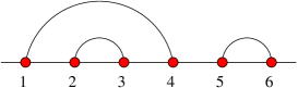
Figure 1. A Standard Young Tableau and the corresponding link pattern.

In this language, one has a rather convenient description of orbital varieties [25, 26], which we mention for the sake of completeness. Indeed, to each orbital variety $\pi$ we associate the upper triangular matrix $\pi^{<}$ with $\pi^{<}_{ij}=1$ if points labelled $i$ and $j$ are connected by an arch, $i<j$, $0$ otherwise. Then $\pi=\overline{B\cdot\pi^{<}}$, $B$ acting by conjugation. Equivalently, $\pi$ is given by the following set of equations: (i) $M^{2}=0$ and (ii) $r_{ij}(M)\leq r_{ij}(\pi^{<})$, $i,j=1,\ldots,N$, where $r_{ij}$ is the rank of the $i\times j$ lower-left rectangle.

$$e_{4}\ \raise-7.39772pt\hbox{\psfig{width=113.81102pt}}=\raise-26.17651pt\hbox{\psfig{width=113.81102pt}}=\raise-7.39772pt\hbox{\psfig{width=113.81102pt}}$$

$$e_{2}\ \raise-7.39772pt\hbox{\psfig{width=113.81102pt}}=\raise-26.17651pt\hbox{\psfig{width=113.81102pt}}=\beta\ \raise-7.39772pt\hbox{\psfig{width=113.81102pt}}$$

Figure 2. Action of the Temperley–Lieb algebra $TL(\beta)$ on link patterns.

It is equally simple to describe the action of the Weyl group, namely the symmetric group $S_{N}$. Rather than the generators corresponding to the simple roots: $s_{i}\equiv s_{\alpha_{i}}$, $i=1,\ldots,r$ used so far, it proves simpler to consider the action of the projectors $e_{i}=1-s_{i}$ in the symmetric group algebra. The operator $e_{i}$ acts on link patterns $\pi$ by connecting the arches ending at $i$ and $i+1$ and creates a new little arch between these 2 points; this action is described on Fig. 2. When a closed loop is formed, it is erased but contributes a weight $\beta=2$. The $q$-deformed version of this is obtained by attaching a weight $\beta=-(q+q^{-1})$ to each erased loop, thus leading to the following (pictorially clear) relations:

(3.1) $$e_{i}^{2}=\beta e_{i}\qquad e_{i}=e_{i}e_{i\pm 1}e_{i}\qquad[e_{i},e_{j}]=0\quad|i-j|>1$$

all indices taking values in $1,\ldots,r$. These are the defining relations of the Temperley–Lieb algebra $TL_{r+1}(\beta)$. When $q=-1$, i.e. $\beta=2$, it is simply a quotient of the symmetric group algebra. Alternatively, the deformed generators $s_{i}=-q^{-1}-e_{i}$ satisfy the usual relations of the Hecke algebra (of which the Temperley–Lieb algebra is a quotient).

In what follows, one special element of $TL_{N}(\beta)$ will be needed: it is the cyclic rotation $S$. Its effect is to rotate the endpoints of the link patterns: $1\to 2\to\cdots\to N\to 1$ without changing their connectivity. It can also be expressed as: $S=q^{n-2}s_{1}\cdots s_{N-1}$.

3.2. $q$KZ equation

For each simple root $\alpha_{i}$, we have the trigonometric $R$-matrix:

(3.2) $$R_{i}(w)\equiv R_{\alpha_{i}}(w)={(qw-q^{-1})+(w-1)e_{i}\over q-q^{-1}w},$$

where the $e_{i}=-q^{-1}-s_{i}$ generate $TL_{N}(\beta)$ and act in the space of link patterns as explained above. We first write the system of equations:

(3.3) $$R_{i}(w_{i+1}/w_{i})\Psi=\tau_{i}\Psi\qquad i=1,\ldots,N-1$$

where $\tau_{i}\equiv\tau_{\alpha_{i}}$ acts by interchanging multiplicative spectral parameters $w_{i}:=e^{-\hbar z_{i}}$ and $w_{i+1}$ in the polynomial $\Psi$ of the $w$’s, homogeneous of degree $n(n-1)$.

These equations are supplemented by the “affinized” equation satisfied by $\Psi$. Since the affine Dynkin diagram $A_{r}^{(1)}$ is a circular chain, this equation quite naturally involves the cyclic rotation $S$. Define the operator $\rho$ on $\mathbb{C}[w_{1},\ldots,w_{N}]$ which shifts the variables $w_{i}$ according to the rule: $w_{i}\to w_{i+1}$, $i=1,\ldots,N-1$ and $w_{N}\to q^{6}w_{1}$. Then the additional equation is

(3.4) $$q^{3(n-1)}S^{-1}\Psi=\rho\Psi$$

Together with this equation, the above system forms the so-called level one $q$KZ equation.

We claim that the ${\bf R}_{i}:=\tau_{i}R_{i}(w_{i+1}/w_{i})$ and ${\bf S}:=q^{3(1-n)}\rho S$ generate together $\hat{W}$. In order to see that, it is sufficient to build the $N$ generators ${\bf T}_{i}$ of the abelian subgroup (the lattice of weights). They are given by ${\bf T}_{i}={\bf R}_{i-1}{\bf R}_{i-2}\cdots{\bf R}_{1}{\bf S}{\bf R}_{N-1}\cdots{\bf R}_{i+1}{\bf R}_{i}$, $i=1,\ldots,N$. The original definition of the $q$KZ equation is in fact the eigenvector equation for these “scattering” matrices; with reasonable assumptions it is equivalent to the above system. Also, note that if one defines ${\bf R}_{N}:={\bf S}^{-1}{\bf R}_{1}{\bf S}$, then the ${\bf R}_{i}$, $i=1,\ldots,N$ generate the usual affine Weyl group (a subgroup of order $N$ of $\hat{W}$).

The minimal degree polynomial solution of the level one $q$KZ equation was obtained in [6, 7], and is characterized by its “base” entry $\Psi_{\pi_{0}}$ corresponding to the link pattern $\pi_{0}$ that connects points $i\leftrightarrow 2n+1-i$, with the value

(3.5) $$\Psi_{\pi_{0}}=\prod_{1\leq i<j\leq n}(qw_{i}-q^{-1}w_{j})\prod_{n+1\leq i<j\leq 2n}(qw_{i}-q^{-1}w_{j})$$

in which all factors are a direct consequence of the $\tau_{i}\Psi=R_{i}\Psi$ equations. It is then easy to prove that all the other entries of $\Psi$ may be obtained from $\Psi_{\pi_{0}}$ in a triangular way.

Example: at $N=6$, there are 5 link patterns. The minimal degree polynomial solution of the level one $q$KZ equation reads:

$$\Psi_{\psfig{width=51.21504pt}}=(qw_{1}-q^{-1}w_{2})(qw_{2}-q^{-1}w_{3})(qw_{1}-q^{-1}w_{3})(qw_{4}-q^{-1}w_{5})(qw_{5}-q^{-1}w_{6})(qw_{4}-q^{-1}w_{6})$$

$$\Psi_{\psfig{width=51.21504pt}}=(qw_{1}-q^{-1}w_{2})(qw_{3}-q^{-1}w_{4})(qw_{5}-q^{-1}w_{6})$$

$$\times\Big{(}(w_{1}+w_{2})(q^{2}w_{3}w_{4}-q^{-2}w_{5}w_{6})-(w_{3}+w_{4})(q^{4}w_{1}w_{2}-q^{-4}w_{5}w_{6})+(w_{5}+w_{6})(q^{2}w_{1}w_{2}-q^{-2}w_{3}w_{4})\Big{)}$$

$$\Psi_{\psfig{width=51.21504pt}}=(qw_{2}-q^{-1}w_{3})(qw_{2}-q^{-1}w_{4})(qw_{3}-q^{-1}w_{4})(qw_{5}-q^{-1}w_{6})(q^{-2}w_{6}-q^{2}w_{1})(q^{-2}w_{5}-q^{2}w_{1})$$

$$\Psi_{\psfig{width=51.21504pt}}=(qw_{1}-q^{-1}w_{2})(qw_{3}-q^{-1}w_{4})(qw_{4}-q^{-1}w_{5})(qw_{3}-q^{-1}w_{5})(q^{-2}w_{6}-q^{2}w_{1})(q^{-2}w_{6}-q^{2}w_{2})$$

$$\Psi_{\psfig{width=51.21504pt}}=(qw_{2}-q^{-1}w_{3})(qw_{4}-q^{-1}w_{5})(q^{-2}w_{6}-q^{2}w_{1})$$

$$\times\Big{(}(q^{3}w_{1}+q^{-3}w_{6})(q^{2}w_{2}w_{3}-q^{-2}w_{4}w_{5})-(w_{2}+w_{3})(qw_{1}w_{6}-q^{-1}w_{4}w_{5})-(w_{4}+w_{5})(qw_{2}w_{3}-q^{-1}w_{1}w_{6})\Big{)}$$

Performing the rational limit $\hbar\to 0$, $z_{i}=e^{-\hbar w_{i}}$, $q=-e^{-\hbar A/2}$ yields the following multidegrees:

$$\Psi_{\psfig{width=51.21504pt}}=(A+z_{1}-z_{2})(A+z_{2}-z_{3})(A+z_{1}-z_{3})(A+z_{4}-z_{5})(A+z_{5}-z_{6})(A+z_{4}-z_{6})$$

$$\Psi_{\psfig{width=51.21504pt}}=(A+z_{1}-z_{2})(A+z_{3}-z_{4})(A+z_{5}-z_{6})\Big{(}4A^{3}+3A^{2}(z_{1}+z_{2}-z_{5}-z_{6})+$$

$$+A(2(z_{1}z_{2}-2z_{3}z_{4}-z_{1}z_{5}-z_{2}z_{5}-z_{1}z_{6}-z_{2}z_{6}+z_{5}z_{6})+(z_{3}+z_{4})(z_{1}+z_{2}+z_{5}+z_{6}))$$

$$+(z_{1}+z_{2})(z_{5}z_{6}-z_{3}z_{4})+(z_{3}+z_{4})(z_{1}z_{2}-z_{5}z_{6})+(z_{5}+z_{6})(z_{3}z_{4}-z_{1}z_{2})\Big{)}$$

$$\Psi_{\psfig{width=51.21504pt}}=(A+z_{2}-z_{3})(A+z_{2}-z_{4})(A+z_{3}-z_{4})(A+z_{5}-z_{6})(2A+z_{1}-z_{6})(2A+z_{1}-z_{5})$$

$$\Psi_{\psfig{width=51.21504pt}}=(A+z_{1}-z_{2})(A+z_{3}-z_{4})(A+z_{4}-z_{5})(A+z_{3}-z_{5})(2A+z_{1}-z_{6})(2A+z_{2}-z_{6})$$

$$\Psi_{\psfig{width=51.21504pt}}=(A+z_{2}-z_{3})(A+z_{4}-z_{5})(2A+z_{1}-z_{6})\Big{(}5A^{3}+3A^{2}(z_{1}+z_{2}+z_{3}-z_{4}-z_{5}-z_{6})+$$

$$+A(2z_{1}(z_{2}+z_{3}-z_{6})+z_{2}z_{3}+z_{4}z_{5}-(z_{2}+z_{3})z_{6}+(z_{4}+z_{5})(2z_{6}-z_{1}-z_{2}-z_{3}))$$

$$+(z_{1}+z_{6})(z_{2}z_{3}-z_{4}z_{5})+(z_{2}+z_{3})(z_{4}z_{5}-z_{1}z_{6})+(z_{4}+z_{5})(z_{1}z_{6}-z_{2}z_{3})\Big{)}$$

and in particular the degrees $1,4,4,4,10$ respectively, upon taking $z_{i}=0$ and $A=1$.

3.3. Razumov–Stroganov point and ASM

At $q=e^{2i\pi/3}$, $\Psi$ becomes the ground state eigenvector of the integrable transfer matrix with periodic boundary conditions and inhomogeneities $w_{1}$, $\ldots$, $w_{N}$, or equivalently of the scattering matrices ${\bf T}_{i}=R_{i-1}(w_{i-1}/w_{i})\cdots R_{1}(w_{1}/w_{i})SR_{N-1}(w_{N-1}/w_{i})\cdots R_{i}(w_{i+1}/w_{i})$. Consider now the particular case $w_{1}=\cdots=w_{N}=1$, when $\Psi$ is the Perron–Frobenius eigenvector of the Hamiltonian $H=e_{1}+\cdots+e_{N}$ where $e_{N}=S^{-1}e_{1}S$. Note that the periodic boundary conditions mean that $H$ is cyclic-invariant: $SH=HS$. Normalizing $\Psi$ so that its smallest entry $\Psi_{\pi_{0}}$ is $1$, we have the following

Theorem.

[4] The sum of entries $\sum_{\pi}\Psi_{\pi}$ is equal to the number of Alternating Sign Matrices, $A(n)$.

The result of [4] is actually much more general, as the sum $\sum_{\pi}\Psi_{\pi}$ was evaluated in the presence of all the spectral parameters $w_{i}$, and identified with proper normalization to the so-called Izergin–Korepin determinant [20, 21], also equal to a particular Schur function [22]. Still unproven, however, is the

Conjecture.

[1] The largest entry of $\Psi$, with arches connecting consecutive points, is $A(n-1)$.

For instance, plugging $w_{i}=1$ and $q=e^{2i\pi/3}$ into the above example, we get for $N=6$, $\Psi=(1,2,1,1,2)$ and $\sum_{\pi}\Psi_{\pi}=7=A(3)$, the total number of $3\times 3$ ASMs.

4. $B_{r}$ case

We now develop the $B_{r}$ case, which allows us to recover and interpret geometrically the results of [16]. We concentrate on the even case $r=2n$. We parametrize as usual the roots $\alpha_{i}=z_{i}-z_{i+1}$ for $i=1,2,\ldots,r-1$ and $\alpha_{r}=z_{r}$.

We consider matrices that square to zero in the fundamental representation of dimension $N=2r+1$: a possible choice is to select upper triangular matrices satisfying $M^{T}J+JM=0$, $J$ antidiagonal matrix with 1’s on the second diagonal. It turns out that the orbital varieties are indexed by the same link patterns as before, of size $r$; and that the Weyl group representation is actually a representation of the same quotient, the Temperley–Lieb algebra $TL_{r}(\beta)$, the additional reflection $s_{r}$ being represented by a multiple of the identity.

4.1. $B$-type $q$KZ equation

According to the dicusssion above, the B $q$KZ system reads:

(4.1) $$R_{i}(w_{i+1}/w_{i})\Psi = \tau_{i}\Psi,\quad i=1,2,...,r-1$$

(4.2) $$w_{r}^{-m_{r}}{q^{-1}w_{r}-q\over q^{-1}-qw_{r}}\Psi = \tau_{r}\Psi$$

where $\tau_{r}$ stands for the inversion of the last spectral parameter, namely $\tau_{r}\Psi(w_{1},...w_{r-1},w_{r})=\Psi(w_{1},...,w_{r-1},1/w_{r})$ and $m_{r}$ is the degree of $\Psi$ in $w_{r}$.

Finally, these equations are to be supplemented by the affinization relation. The latter is expressed by considering the reflection with respect to the extra root $z_{1}$. One finds that

(4.3) $$(q^{3}w_{1})^{-m_{1}}{q^{-2}-q^{2}w_{1}\over qw_{1}-q^{-1}}\Psi(w_{1},w_{2},...,w_{r})=\Psi\Big{(}{1\over q^{6}w_{1}},w_{2},...,w_{r}\Big{)}$$

where $m_{1}$ is the degree of $\Psi$ in $z_{1}$.

Introducing the boundary operators ${\bf K}_{1}$ and ${\bf K}_{r}$ so that Eqs. (4.2–4.3) reduce to ${\bf K}_{1}\Psi={\bf K}_{2}\Psi=\Psi$, as well as the usual ${\bf R}_{i}=\tau_{i}R_{i}(w_{i+1}/w_{i})$, the generators of the weight lattice (as abelian subgroup of $\hat{W}$) are: (i) ${\bf T}_{i}={\bf R}_{i}{\bf R}_{i+1}\cdots{\bf R}_{r-1}{\bf K}_{r}{\bf R}_{r-1}\cdots$ ${\bf R}_{1}{\bf K}_{1}{\bf R}_{1}\cdots{\bf R}_{i-1}$ that implements $w_{i}\to q^{6}w_{i}$ and (ii) one additional generator implementing $w_{i}\to q^{3}w_{i}$ simultaneously for all $i$. The latter is a combination of R and K matrices as well as an additional operator implementing the reflection $w_{i}\leftrightarrow q^{-3}/w_{r+1-i}$ for all $i$.

The minimal polynomial solution to the system (4.1–4.3) has degree $m_{1}=m_{r}=r-1=2n-1$ in each spectral parameter and total degree $n(3n-1)$. As before it has a simple factorized base entry

(4.4) $$\Psi_{\pi_{0}}=C\prod_{1\leq i<j\leq n}(qw_{i}-q^{-1}w_{j})(q^{-2}-q^{2}w_{i}w_{j})\prod_{n+1\leq i<j\leq 2n}(qw_{i}-q^{-1}w_{j})(qw_{i}w_{j}-q^{-1})$$

where $C=2^{n}\prod_{i=1}^{r}(qw_{i}-q^{-1})$ is a common (symmetric) factor to all entries of $\Psi$. All other entries may be obtained from this one in a triangular manner.

Example: For $B_{4}$, there are 2 link patterns as for the case $A_{3}$. The minimal degree polynomial solution of the level one $B_{4}$ $q$KZ equation reads:

$$\Psi_{\psfig{width=34.14322pt}}=C(qw_{1}-q^{-1}w_{2})(q^{-2}-q^{2}w_{1}w_{2})(qw_{3}-q^{-1}w_{4})(qw_{3}w_{4}-q^{-1})$$

$$\Psi_{\psfig{width=34.14322pt}}=C(qw_{2}-q^{-1}w_{3})(q^{-1}w_{1}-qw_{1}w_{2}w_{3}-q^{-5}w_{4}-qw_{1}^{2}w_{4}+(q^{-1}-q)w_{1}(w_{2}+w_{3})w_{4}$$

$$\ \ \ +q^{-1}w_{2}w_{3}w_{4}+q^{5}w_{1}^{2}w_{2}w_{3}w_{4}+q^{-1}w_{1}w_{4}^{2}-qw_{1}w_{2}w_{3}w_{4}^{2})$$

As before, we get the corresponding multidegrees upon taking the rational limit, with the result:

$$\Psi_{\psfig{width=34.14322pt}}=C^{\prime}(A+z_{1}-z_{2})(2A+z_{1}+z_{2})(A+z_{3}-z_{4})(A+z_{3}+z_{4})$$

$$\Psi_{\psfig{width=34.14322pt}}=C^{\prime}(A+z_{2}-z_{3})\Big{(}5A^{3}+3A^{2}(2z_{1}+z_{2}+z_{3})+A(2z_{1}^{2}+3z_{1}(z_{2}+z_{3})+z_{2}z_{3}-z_{4}^{2})$$

$$+(z_{2}+z_{3})(z_{1}^{2}-z_{4}^{2})\Big{)}$$

with $C^{\prime}=4(A+z_{1})(A+z_{2})(A+z_{3})(A+z_{4})$; hence the degrees $4\times 2,4\times 5$ for $A=1$ and $z_{i}=0$.

4.2. RS point, VSASM and CSTCPP

As explained in Sect. 2, the case $q=e^{2i\pi/3}$ is special in that the problem admits a transfer matrix, and its solution $\Psi$ in the homogeneous limit where all $w_{i}=1$ is the groundstate of a Hamiltonian

(4.5) $$H_{B}=e_{1}+e_{2}+...+e_{N-1}$$

which is the open boundary version of the $A_{r}$ Hamiltonian $H$.

As shown in [17], at the RS point $q=e^{2i\pi/3}$, and in the homogeneous limit where $w_{i}=1$ for all $i$, and in which $\Psi$ is normalized so that its smallest entry is $\Psi_{\pi_{0}}=1$, we have the following

Theorem.

[16] The sum of entries $\sum_{\pi}\Psi_{\pi}$ is equal to the number of Vertically Symmetric Alternating Sign Matrices (VSASM), $A_{V}(2n+1)$.

This was actually proved in the same spirit as for the $A_{r}$ case, by identifying the sum of components including all spectral parameters $w_{i}$ as yet another determinant, which takes the form of a particular symplectic Schur function. A similar result holds for the case of odd $r=2n-1$, namely once properly normalized, the sum of entries $\sum_{\pi}\Psi_{\pi}$ is equal to an integer we call $A_{V}(2n)$ by analogy. It turns out that $A_{V}(2n)=N_{8}(2n)$ is the number of Cyclically Symmetric Transpose Complement Plane Partitions (CSTCPP) in an hexagon of size $2n\times 2n\times 2n$ [24]. The numbers $A_{V}(i)$ both have determinant formulae, namely $A_{V}(2n)=\det{i+j\choose 2i-j}_{0\leq i,j\leq n-1}$, and $A_{V}(2n+1)=\det{i+j+1\choose 2i-j}_{0\leq i,j\leq n-1}$.

As in the $A$ case, we have the

Conjecture.

[1] The largest entry of $\Psi$, with arches connecting consecutive points, is $A_{V}(r)$.

Example: for $r=2n=4$, taking $w_{i}\to 1$ and $q=e^{2i\pi/3}$ in the above expressions, we get the components $\Psi=(1,2)$, which sum to $3=A_{V}(5)$, the number of $5\times 5$ VSASMs, and the maximal entry of $\Psi$ is $2=N_{8}(4)$.

5. $C_{r}$ case

The simple roots of $C_{r}$ are $\alpha_{i}=z_{i}-z_{i+1}$, $i=1,2,\ldots,r-1$ and $\alpha_{r}=2z_{r}$. We concentrate on the odd case $r=2n+1$, and consider the fundamental representation of dimension $N=2r$. One choice is to select upper triangular matrices satisfying $M^{T}J+JM=0$, $J$ antidiagonal matrix with $1$’s (resp. $-1$’s) in the upper (resp. lower) triangle.

5.1. Orbital varieties and $C$-type Temperley–Lieb algebra

There are $r\choose\lfloor{r+1\over 2}\rfloor$ orbital varieties, which are now indexed by open link patterns, that is configurations of $r$ points on a line connected in the upper-half plane either in pairs via (closed) arches or to infinity via half-lines (open arches).

The representation of the Weyl group on these open link patterns takes the form of a modified Temperley–Lieb algebra. We describe now its $q$-deformed version, $CTL(\beta)$ (see also [23] for other variants of Temperley–Lieb algebra). The generators $e_{1},e_{2},\ldots,e_{r-1}$ obey the standard $TL(\beta)$ relations (3.1) and the additional “boundary” generator $e_{r}$ satisfies: $e_{r}^{2}=\beta e_{r}$, $e_{r-1}e_{r}e_{r-1}=2e_{r-1}$.

These generators act on open link patterns as follows. Open link patterns are represented with their open arches connected to a vertical line on the right. The $e_{i}$, $i=1,2,...,r-1$ act as usual, and $e_{r}$ like the left half of an $e$, connecting the point $2n+1$ to the vertical line (first line of Fig. 3). The rule is that any loop may be erased and replaced by a factor $\beta$. Moreover, whenever a connection between points on the vertical line (consecutive open arches) is created, they may also be erased and replaced by a factor $\beta$ (resp. $2$) if this is created by the action of some $e_{2i-1}$ (resp. $e_{2i}$). As $r$ is odd, the loop created by $e_{r}^{2}$ yields a weight $\beta$, while that created by $e_{r-1}e_{r}e_{r-1}$ yields a weight $2$, hence the result $2e_{n-1}$ (second line of Fig. 3).

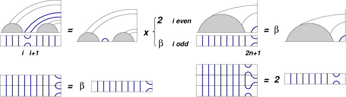
Figure 3. The rule for erasing arches at infinity when acting with $e_{i}$: they are replaced by a factor $2$ (resp. $\beta$) according to whether the index $i$ is even (resp. odd). We have also represented the case $i=2n+1$ (first line), and the resulting boundary relations $e_{r}^{2}=\beta e_{r}$ and $e_{r-1}e_{r}e_{r-1}=2e_{r-1}$ (second line).

We shall also need an additional operator $e_{1}^{\prime}$ satisfying the relations: $(e_{1}^{\prime})^{2}=\beta e_{1}^{\prime}$ and $e_{1}e_{1}^{\prime}=e_{1}^{\prime}e_{1}=e_{1}^{\prime}e_{2}e_{1}^{\prime}-e_{1}^{\prime}=e_{2}e_{1}^{\prime}e_{2}-e_{2}=0$. It is defined as $e^{\prime}_{1}=se_{1}s$, where $s$ is the involution acting on link patterns as follows: (i) $s\pi=\pi$ if the arch connected to point $1$ is open, and (ii) $s\pi=-\pi+\pi^{\prime}$ otherwise, where $\pi^{\prime}$ is the link pattern in which the closed arch connected to $1$ is cut into two open arches.

5.2. $C$-type $q$KZ equation

To each simple root we attach respectively the standard trigonometric $R$-matrices $R_{i}(w_{i+1}/w_{i})$, $i=1,2,\ldots,r-1$ of Eq. (3.2), and the boundary $R$-matrix $R_{r}(1/w_{r}^{2})\equiv R_{\alpha_{r}}$, with the same expression.

The level one $C$ $q$KZ equation consists of the following system

(5.1) $$R_{i}(w_{i+1}/w_{i})\Psi =\tau_{i}\Psi$$

(5.2) $$w_{r}^{-m_{r}}R_{r}(1/w_{r}^{2})\Psi =\tau_{r}\Psi$$

where as usual $\tau_{i}$ acts by interchanging the spectral parameters $w_{i}$ and $w_{i+1}$, $i=1,2,...,r-1$ and $\tau_{r}$ acts on $\Psi$ by letting $w_{r}\to 1/w_{r}$, and $m_{r}$ is the degree of $\Psi$ in $w_{r}$.

These are finally supplemented by the affinization relation, obtained by considering an extra root, say $\alpha_{1}^{\prime}=-z_{1}-z_{2}$, and the associated boundary operator $R_{1}^{\prime}(q^{6}w_{1}w_{2})$:

(5.3) $$R_{1}^{\prime}(q^{6}w_{1}w_{2})\Psi=\tau_{1}^{\prime}\Psi$$

where $\tau_{1}^{\prime}$ interchanges $w_{2}$ and $1/(q^{6}w_{1})$, and $R^{\prime}_{1}$ is of the form of Eq. (3.2) with $e^{\prime}_{1}$ in place of $e_{i}$. Using $R^{\prime}_{1}(w)=sR_{1}(w)s$, the relation can also be recast into

(5.4) $$(q^{3}z_{1})^{-m_{1}}s\Psi(w_{1},\ldots,w_{r})=\Psi\Big{(}{1\over q^{6}w_{1}},w_{2},\ldots,w_{r})$$

The generators of the weight lattice (as abelian subgroup of $\hat{W}$) are very similar to the generators (i) of the case $B_{r}$: the only change concerns the boundary operators ${\bf K}_{1}$ and ${\bf K}_{r}$ now implementing Eqs. (5.2) and (5.4).

The polynomial solution $\Psi$ to the level one $C_{r}$ $q$KZ system has degree $m_{1}=m_{r}=2n$ in each variable, total degree $n(2n+1)$ and base entry

(5.5) $$\Psi_{\pi_{0}}=\prod_{1\leq i<j\leq 2n+1}(qz_{i}-q^{-1}z_{j})$$

and all the other entries of $\Psi$ may be obtained in a triangular way from this one.

Example: for $r=3$, we have the following minimal polynomial solution to the level one $C_{3}$ $q$KZ system:

$$\Psi_{\psfig{width=25.6073pt}}=(qw_{1}-q^{-1}w_{2})(qw_{1}-q^{-1}w_{3})(qw_{2}-q^{-1}w_{3})$$

$$\Psi_{\psfig{width=25.6073pt}}=(qw_{1}-q^{-1}w_{2})(q^{2}w_{1}w_{2}-q^{-2})(q^{-1}-qw_{3}^{2})$$

$$\Psi_{\psfig{width=25.6073pt}}=(q^{3}w_{1}^{2}-q^{-3})(qw_{2}-q^{-1}w_{3})(qw_{2}w_{3}-q^{-1})$$

which, upon taking the rational limit yields the multidegrees:

$$\Psi_{\psfig{width=25.6073pt}}=(A+z_{1}-z_{2})(A+z_{1}-z_{3})(A+z_{2}-z_{3})$$

$$\Psi_{\psfig{width=25.6073pt}}=(A+z_{1}-z_{2})(2A+z_{1}+z_{2})(A+2z_{3})$$

$$\Psi_{\psfig{width=25.6073pt}}=(3A+2z_{1})(A+z_{2}-z_{3})(A+z_{2}+z_{3})$$

and the degrees $\Psi=(1,2,3)$ for $A=1$ and $z_{i}=0$.

5.3. RS point and CSSCPP

At the point $q=e^{2i\pi/3}$, $\Psi$ may be viewed as the ground state eigenvector of a transfer matrix, corresponding in the homogeneous limit to the Hamiltonian

(5.6) $$H_{C}={e_{1}+e_{1}^{\prime}\over 2}+\sum_{i=2}^{r-1}e_{i}+e_{r}$$

Normalizing $\Psi$ so that its smallest entry $\Psi_{\pi_{0}}=1$, we have been able to compute the sum of entries to be $A(n)A(n+1)$. In the case of even $r=2n$, the above may be repeated almost identically: in the presence of spectral parameters, the even case may be recovered from the odd one by taking $w_{2n+1}\to-q^{-1}$, and dividing out the result by $\prod_{1\leq i\leq 2n}(1+q^{3}w_{i})$. Indeed, this specialization leaves us with only non-vanishing components whith an open arch at the rightmost point, in bijection with open link patterns with that point erased, hence the projection onto the case of size one less. This leads us to the

Conjecture.

(5.7) $$\sum_{\pi}\Psi_{\pi}=A(\lfloor r/2\rfloor)A(\lceil r/2\rceil)$$

Note that the sum in the even case, $A(n)^{2}$, also counts the Cyclically Symmetric Self-Complementary Plane Partitions (CSSCPP) in an hexagon of size $2n\times 2n\times 2n$ [24]. Also note the determinant formulae $A(n)^{2}=\det\Big{(}{i+j\choose 2i-j-1}+{i+j+1\choose 2i-j}\Big{)}_{0\leq i,j\leq n-1}$ and $A(n)A(n+1)=\det\Big{(}{i+j+1\choose 2i-j}+{i+j+2\choose 2i-j}\Big{)}_{0\leq i,j\leq n-1}$.

Furthermore, consider the left eigenvector $v$ of $H_{C}$ with the same eigenvalue ($r$ for $r$ odd, $r+1/2$ for $r$ even). Normalize $v$ so that its entries are coprime positive integers. We have found empirically the following

Conjecture.

(5.8) $$\sum_{\pi}v_{\pi}\Psi_{\pi}=A(r)\ .$$

Finally, we formulate the

Conjecture.

The largest entry of $\Psi$ for $C_{r}$ is the sum of entries for $C_{r-1}$.

Example: at $r=5$, $\Psi=(1,2,3,3,0,1,4,0,0,0)$, $v=(48,36,28,34,24,23,25,18,17,14)$, $\sum_{\pi}\Psi_{\pi}=14=2\times 7=A(2)A(3)$, $\sum_{\pi}v_{\pi}\Psi_{\pi}=429=A(5)$, and the maximal entry of $\Psi$ is $4=A(2)^{2}$.

6. $D_{r}$ case

The simple roots of $D_{r}$ are $\alpha_{i}=z_{i}-z_{i+1}$ for $i=1,2,\ldots,n-1$ and $\alpha_{r}=z_{r-1}+z_{r}$. We concentrate on the odd case $r=2n+1$, and consider again the fundamental representation of dimension $N=2r$. Just like in the $B_{r}$ case, one choice is to select upper triangular matrices satisfying $M^{T}J+JM=0$, $J$ antidiagonal matrix with $1$’s on the second diagonal.

6.1. Orbital varieties and $D$-type Temperley–Lieb algebra

Just as in the case $C$, there are $r\choose\lfloor{r+1\over 2}\rfloor$ orbital varieties, indexed by open link patterns.

We now deal with $D$-type Temperley–Lieb algebras, denoted $DTL(\beta)$, with generators $e_{i}$, $i=1,2,...,r-1$ obeying the $TL(\beta)$ relations (3.1) and an extra generator $e_{r-1}^{\prime}$, satisfying the relations:

(6.1) $$(e_{r-1}^{\prime})^{2}=\beta e_{r-1},\qquad e_{r-1}e_{r-1}^{\prime}=e_{r-1}^{\prime}e_{r-1}=e_{r-2}e_{r-1}^{\prime}e_{r-2}-e_{r-2}=e_{r-1}^{\prime}e_{r-2}e_{r-1}^{\prime}-e_{r-1}^{\prime}=0$$

These operators act on open link patterns as follows. The $e_{i}$, $i=1,2,\ldots,r-1$ act in the usual way, by creating a little arch between points $i$ and $i+1$ and by gluing the two former points. To describe the action of $e_{r-1}^{\prime}$, let us first connect the open arches of the open link patterns by pairs of consecutive open arches from the left to the right, and represent the newly formed arches in a different color (dashed lines, cf Fig. 4 for the $D_{5}$ example). We then define an involution $s$ on open link patterns that simply switches the color (solid $\leftrightarrow$ dashed) of the rightmost arch if it is closed, and leaves it invariant if it is open. Then $e_{r-1}^{\prime}=se_{r-1}s$.

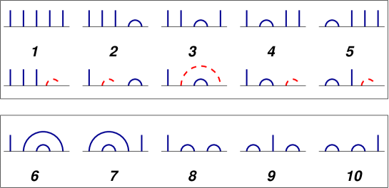
Figure 4. The ten open link patterns for $D_{5}$. In the second line, we have transformed the open link patterns by connecting the two rightmost open arches into a (dashed) arch. The involution $s$ simply switches the color of the rightmost arch (if it is closed) in this representation, namley exchanges $1\leftrightarrow 2$, $3\leftrightarrow 6$, $4\leftrightarrow 8$, $5\leftrightarrow 9$, and leaves $7$ and $10$ invariant (as their rightmost arch is open).

Finally, we introduce an extra boundary operator $e_{0}$, which is the right half of an $e$ (like a reflected $e_{r}$ of $C_{r}$), with its open end connected to the vertical line, and acts as such, with the same rules as for $C_{r}$, but upon reflection of indices $i\leftrightarrow r-i$. It satisfies the relations: $e_{0}^{2}=\beta e_{0}$ and $e_{1}e_{0}e_{1}=2e_{1}$.

6.2. $D$-type $q$KZ equation

We associate to the roots the $R$-matrices $R_{i}(w_{i+1}/w_{i})$ of Eq. (3.2), and $R_{r}(1/(w_{r}w_{r-1}))$ defined by the same equation in which $e_{i}$ is replaced with $e^{\prime}_{r-1}$, so that $R_{r}(w)=sR_{r-1}(w)s$.

The level one $D$ $q$KZ equation consists of the following system

$$R_{i}(w_{i+1}/w_{i})\Psi =\tau_{i}\Psi,\qquad i=1,2,...,r-1$$

$$R_{r}(1/(w_{r}w_{r-1}))\Psi =\tau_{r-1}^{\prime}\Psi$$

where as usual $\tau_{i}$ acts by interchanging the spectral parameters $w_{i}$ and $w_{i+1}$, $i=1,2,...,r-1$ and $\tau_{r}^{\prime}$ acts on $\Psi$ by interchanging $w_{r-1}$ and $1/w_{r}$. Upon using the above relation $e_{r-1}^{\prime}=se_{r-1}s$, the latter equation may be equivalently replaced by

(6.2) $$z_{r}^{-m_{r}}s\Psi(z_{1},\ldots,z_{r})=\Psi\Big{(}z_{1},\ldots,z_{r-1},{1\over z_{r}}\Big{)}$$

These are finally supplemented by the affinization relation, obtained by considering the extra root $\alpha_{0}=-2z_{1}$, and the associated boundary operator $R_{0}(q^{6}w_{1}^{2})$ involving the extra operator $e_{0}$:

(6.3) $$w_{1}^{-m_{1}}R_{0}(q^{6}w_{1}^{2})\Psi=\tau_{0}\Psi$$

where $\tau_{0}f(w_{1})=f(1/(q^{6}w_{1}))$ and $m_{1}$ the degree of $\Psi$ in $w_{1}$.

The construction of the abelian subgroup of $\hat{W}$ is similar to the cases $B$ and $C$, and is skipped for the sake of brevity.

The minimal degree polynomial solution to the level one $D_{r}$ $q$KZ system has total degree $r(r-1)/2$ and partial degree $m_{1}=m_{r}=r-1$ in all variables. Its base entry, corresponding to the open link pattern $\pi_{0}$ with only open arches reads

(6.4) $$\Psi_{\pi_{0}}=\prod_{1\leq i<j\leq 2n+1}(qz_{i}-q^{-1}z_{j})$$

and all the other entries of $\Psi$ may be obtained in a triangular way from this one.

Example: for $r=3$, we have the following minimal polynomial solution to the level one $D_{3}$ $q$KZ system:

$$\Psi_{\psfig{width=25.6073pt}}=(qw_{1}-q^{-1}w_{2})(qw_{1}-q^{-1}w_{3})(qw_{2}-q^{-1}w_{3})$$

$$\Psi_{\psfig{width=25.6073pt}}=(qw_{1}-q^{-1}w_{2})(qw_{1}w_{3}-q^{-1})(qw_{2}w_{3}-q^{-1})$$

$$\Psi_{\psfig{width=25.6073pt}}=(q^{-2}-q^{2}w_{1}^{2})(qw_{2}-q^{-1}w_{3})(qw_{2}w_{3}-q^{-1})$$

which, upon taking the rational limit gives the multidegrees:

$$\Psi_{\psfig{width=25.6073pt}}=(A+z_{1}-z_{2})(A+z_{1}-z_{3})(A+z_{2}-z_{3})$$

$$\Psi_{\psfig{width=25.6073pt}}=(A+z_{1}-z_{2})(A+z_{1}+z_{3})(A+z_{2}+z_{3})$$

$$\Psi_{\psfig{width=25.6073pt}}=2(A+z_{1})(A+z_{2}-z_{3})(A+z_{2}+z_{3})$$

and the degrees $\Psi=(1,1,2)$ for $A=1$ and $z_{i}=0$.

6.3. RS point and HTASM

At the point $q=e^{2i\pi/3}$, $\Psi$ may be viewed as the Perron–Frobenius eigenvector of a transfer matrix, corresponding in the homogeneous limit to the Hamiltonian

(6.5) $$H_{D}=e_{0}+\sum_{i=1}^{r-2}e_{i}+{e_{r-1}+e_{r-1}^{\prime}\over 2}$$

Note that upon the reflection $e_{i}\to e_{r-i}$, this Hamiltonian is mapped onto $H_{C}$: we are dealing with the same algebra, but in different representations.

Going to the RS point $q=e^{2i\pi/3}$ and taking the homogeneous limit $w_{i}=1$ for all $i$, and normalizing $\Psi$ so that its smallest entry is $\Psi_{\pi_{0}}=1$, we have found the

Conjecture.

The sum of entries $\sum_{\pi}\Psi_{\pi}$ is the number of Half-Turn Symmetric Alternating Sign Matrices of size $r$, $A_{HT}(r)$.

This conjecture also works in the even case $r=2n$, which may be obtained from the odd one by taking $z_{1}=-q^{-2}$, shifting all remaining spectral parameters $w_{i}\to w_{i-1}$, $i=2,3,...,2n+1$, and dividing out by $\prod_{1\leq i\leq 2n}(1+z_{i})$. Note the formulae $A_{HT}(2n)=\det\Big{(}{i+j\choose 2i-j}+{i+j+1\choose 2i-j}\Big{)}_{0\leq i,j\leq n-1}$ and $A_{HT}(2n+1)=\det\Big{(}{i+j+1\choose 2i-j}+{i+j+2\choose 2i-j+1}\Big{)}_{0\leq i,j\leq n-1}$.

Introduce as before the left Perron–Frobenius eigenvector $v$ of $H_{D}$ with coprime positive integer entries.

Conjecture.

(6.6) $$\sum_{\pi}v_{\pi}\Psi_{\pi}=A(r)\ .$$

Finally, we also find the

Conjecture.

The largest entry of $\Psi$ for $D_{r}$ is the sum of entries for $C_{r-1}$.

Example: at $r=5$, $\Psi=(1,1,3,4,2,3,1,4,2,4)$, $v=(10,10,17,14,18,17,23,14,18,25)$, $\sum_{\pi}\Psi_{\pi}=25=A_{HT}(5)$, $\sum_{\pi}v_{\pi}\Psi_{\pi}=429=A(5)$, and the maximal entry of $\Psi$ is $4=A(2)^{2}$, the sum of the components of the $C_{4}$ solution.

References

• [1] M.T. Batchelor, J. de Gier and B. Nienhuis, The quantum symmetric XXZ chain at $\Delta=-1/2$, alternating sign matrices and plane partitions, J. Phys. A34 (2001) L265–L270, cond-mat/0101385.
• [2] A.V. Razumov and Yu.G. Stroganov, Spin chains and combinatorics, J. Phys A34 (2001), 3185, cond-mat/0012141; Spin chains and combinatorics: twisted boundary conditions, J. Phys A34 (2001), 5335, cond-mat/0012247.
• [3] A.V. Razumov and Yu.G. Stroganov, Combinatorial nature of ground state vector of $O(1)$ loop model, Theor. Math. Phys. 138 (2004) 333–337; Teor. Mat. Fiz. 138 (2004) 395–400, math.CO/0104216.
• [4] P. Di Francesco and P. Zinn-Justin, Around the Razumov–Stroganov conjecture: proof of a multi-parameter sum rule, E. J. Combi. 12 (1) (2005), R6, math-ph/0410061.
• [5] G. Kuperberg, Another proof of the alternating sign matrix conjecture, Int. Math. Research Notes (1996) 139–150, math.CO/9712207.
• [6] V. Pasquier, Quantum incompressibility and Razumov Stroganov type conjectures, cond-mat/0506075.
• [7] P. Di Francesco and P. Zinn-Justin, Quantum Knizhnik–Zamolodchikov equation, generalized Razumov–Stroganov sum rules and extended Joseph polynomials, to appear in J. Phys. A, math-ph/0508059.
• [8] A. Knutson and P. Zinn-Justin, A scheme related to the Brauer loop model, math.AG/0503224.
• [9] P. Di Francesco and P. Zinn-Justin, Inhomogeneous model of crossing loops and multidegrees of some algebraic varieties, to appear in Commun. Math. Phys. (2005), math-ph/0412031.
• [10] G. Kuperberg, Symmetry classes of alternating-sign matrices under one roof, Ann. of Math. (2) 156 (2002), no. 3, 835–866, math.CO/0008184.
• [11] A. Joseph, On the variety of a highest weight module, J. Algebra 88 (1) (1984), 238–278.
• [12] R. Hotta, On Joseph’s construction of Weyl group representations, Tohoku Math. J. Vol. 36 (1984), 49–74.
• [13] I.B. Frenkel and N. Reshetikhin, Quantum affine Algebras and Holonomic Difference Equations, Commun. Math. Phys. 146 (1992), 1–60.
• [14] M. Jimbo and T. Miwa, Algebraic analysis of Solvable Lattice Models, CBMS Regional Conference Series in Mathematics vol. 85, American Mathematical Society, Providence, 1995.
• [15] P. Di Francesco, A. Knutson and P. Zinn-Justin, Extended Orbital Varieties and the Yang–Baxter equation, work in progress.
• [16] P. Di Francesco, Boundary $q$KZ equation and generalized Razumov–Stroganov sum rules for open IRF models, math-ph/0509011.
• [17] P. Di Francesco, Inhomogenous loop models with open boundaries, J. Phys. A 38 (2005), 6091–6120, math-ph/0504032.
• [18] N. Chriss and V. Ginzburg, Representation Theory and Complex Geometry, Birkhauser 1997.
• [19] V. Pasquier, Scattering matrices and Affine Hecke Algebras, q-alg/9508002.
• [20] A. Izergin, Partition function of the six-vertex model in a finite volume, Sov. Phys. Dokl. 32 (1987) 878-879.
• [21] V. Korepin, Calculation of norms of Bethe wave functions, Comm. Math. Phys. 86 (1982) 391-418.
• [22] S. Okada, Enumeration of Symmetry Classes of Alternating Sign Matrices and Characters of Classical Groups, math.CO/0408234.
• [23] R.M. Green, Generalized Temperley–Lieb algebras and decorated tangles, Journal of Knot Theory and its Ramifications 7 (1998), 155–171.
• [24] D. Bressoud, Proofs and confirmations. The story of the alternating sign matrix conjecture, Cambridge University Press (1999).
• [25] B. Rothbach, unpublished.
• [26] A. Melnikova, Description of B-orbit closures of order 2 in upper-triangular matrices, math.RT/0312290, to appear in Transformation Groups.