Asymptotic Hamiltonian reduction
for the dynamics of a particle on a surface

Abstract

We consider the motion of a particle on a surface which is a small perturbation of the standard sphere. One may qualitatively describe the motion by means of a precessing great circle of the sphere. The observation is employed to derive a subsidiary Hamiltonian system that has the form of equations for the top with a 4-th order Hamiltonian, and provides the detailed asymptotic description of the particle’s motion in terms of graphs on the standard sphere.

I Introduction

The dynamics of a particle which is allowed to move freely, i.e. without the action of external forces, on a smooth surface is the classical problem in analytical dynamics, Wh . It is generally hard to solve. In fact, the four Hamiltonian equations for orbits on a surface can be reduced to a system of two Hamiltonian equations by use of the integral of energy and elimination of time, Wh . But the system obtained in this way may have no further integrals and admit of no exact solutions. Thus, the usual reduction method, Wh , or the momentum map according to the current terminology, does not work. The problem looks even more pessimistic if one aims at drawing a picture of the ensemble of orbits on a surface, for it requires the study of the general form and disposition of orbits on a surface of general shape.

In this paper the surface is supposed to be a perturbed standard sphere. Using the perturbation theory we construct a Hamiltonian system, which enables us to give a fairly detailed picture of the ensemble of orbits by means of graphs on the standard sphere; the vertices of the graphs corresponding to orbits which are asymptotically closed and the edges of the graphs to orbits joining the almost closed ones.

Figure 1: Two coils I, II of an orbit on the surface $\varphi(\vec{x})=0$; vectors $N_{I}$ and $N_{II}$ are the normals to the planes of great circles approximating the coils

To be specific, the central idea relies on the circumstance that if the surface does not differ substantially from a sphere, great circles of the latter may serve a good approximation to orbits of the particle. If segments of an orbit are short enough, one can visualize it as winding up in coils; loops or rings of the coil corresponding to great circles of the sphere, see FIG.1. Hence approximating the successive rings by great circles, we may describe the change in the position of the rings by the precession of a great circle, which in its turn is determined by the normal vector $\vec{L}$ of the plane cutting the sphere by the great circle. To cast this picture in a more quantitative form we may use the fact that the normal vector $\vec{L}$ is the angular momentum of the particle moving on the great circle. Thus, we may use perturbation theory, i.e. averaging method, for determining the motion of the angular momentum.

II Averaged equations of motion

The equations of motion of a particle on a surface given by the equation $\varphi(\vec{x})=0$ can be cast in the form of the equation, Wh , R ,

$$\ddot{\vec{x}}=\lambda\,\frac{\partial\varphi}{\partial\vec{x}}\mbox{.}$$ (1)

The Lagrangian multiplier can be found explicitly , so that the equation of motion, in the form that does not involve $\lambda$, reads

$$\ddot{\vec{x}}=-\frac{\dot{\vec{x}}\cdot\displaystyle\frac{\partial^{2}\varphi}{\partial\vec{x}^{2}}\cdot\,\dot{\vec{x}}}{\left(\displaystyle\frac{\partial\varphi}{\partial\vec{x}}\right)^{2}}\,\frac{\partial\varphi}{\partial\vec{x}}\mbox{.}$$ (2)

In this paper we assume that the equations of the surface be of the form

$$\varphi(\vec{x})=\sum_{i}(x_{i}^{2}+\varepsilon_{i}x_{i}^{4})-1\mbox{,}$$

where $\varepsilon_{i}$ are small. Then equations (2) read

$$\ddot{x_{i}}=-\frac{\sum_{j}(2+12\varepsilon_{j}x_{j}^{2})\dot{x_{j}}^{2}}{\sum_{j}(2x_{j}+4\varepsilon_{j}x_{j}^{3})^{2}}(2x_{i}+4\varepsilon_{i}x_{i}^{3})\mbox{.}$$ (3)

The angular momentum $\vec{L}=\vec{r}\times\vec{p}.$ verifies the equations, which follow from (3)

$$\begin{array}[]{lcl}\dot{L_{1}}=-4\,\displaystyle\frac{\sum_{j}(2+12\varepsilon_{j}x_{j}^{2})\dot{x_{j}}^{2}}{\sum_{j}(2x_{j}+4\varepsilon_{j}x_{j}^{3})^{2}}\,x_{2}x_{3}(\varepsilon_{3}x_{3}^{2}-\varepsilon_{2}x_{2}^{2})\vspace{2mm}\\ \dot{L_{2}}=-4\,\displaystyle\frac{\sum_{j}(2+12\varepsilon_{j}x_{j}^{2})\dot{x_{j}}^{2}}{\sum_{j}(2x_{j}+4\varepsilon_{j}x_{j}^{3})^{2}}\,x_{3}x_{1}(\varepsilon_{1}x_{1}^{2}-\varepsilon_{3}x_{3}^{2})\vspace{2mm}\\ \dot{L_{3}}=-4\,\displaystyle\frac{\sum_{j}(2+12\varepsilon_{j}x_{j}^{2})\dot{x_{j}}^{2}}{\sum_{j}(2x_{j}+4\varepsilon_{j}x_{j}^{3})^{2}}\,x_{1}x_{2}(\varepsilon_{2}x_{2}^{2}-\varepsilon_{1}x_{1}^{2})\mbox{.}\vspace{2mm}\end{array}$$ (4)

The equations given above are exact, in the sense that they do not involve any approximation and do not use the $\varepsilon_{i}$ being small. Their treatment still needs further refining, and this will be done with the help of the method of averaging. Generally, the approach relies on studying the evolution equations for integrals of motion of the unperturbed system, i.e. in our case the normals to the planes of the large circles, with respect to the basic periodic solution of the latter. The averaging serves as a filter separating the main regular part of the solution from the oscillating one caused by small terms considered as perturbation, see H .

We may write the basic equation for the particle’s motion on the sphere of unit radius in the form

$$\vec{x}=cos(\omega t+\theta)\vec{e}_{1}+sin(\omega t+\theta)\vec{e}_{2}$$

where vectors $\vec{e}_{1},\vec{e}_{2},\vec{e}_{3}$ can be conveniently taken in the form

$$\begin{array}[]{lcl}\vec{e}_{1}=\displaystyle\frac{1}{\sqrt{L_{2}^{2}+L_{3}^{2}}}(0,L_{3},-L_{2})\vspace{2mm}\\ \vec{e}_{2}=\displaystyle\frac{1}{L\sqrt{L_{2}^{2}+L_{3}^{2}}}(-L_{2}^{2}-L_{3}^{2},L_{1}L_{2},L_{1}L_{3})\vspace{2mm}\\ \vec{e}_{3}=\displaystyle\frac{1}{L}(L_{1},L_{2},L_{3})\mbox{.}\end{array}$$

The angular velocity $\omega$ is given by the equation $\omega^{2}=\dot{\vec{x}}^{2}=L^{2}$, valid to within the first order of perturbation. Here $L_{1},L_{2},L_{3}$ are coordinates of the normal to the plane of the great circle determining the solution, i.e. the angular momentum.

Let us turn to the exact equations for the angular momentum (4). With the help of the equations given above and neglecting terms of the second, and higher, order in the $\varepsilon_{i}$, we can transform equations (4) in the form

$$\begin{array}[]{rcl}\dot{L_{1}}=\displaystyle\frac{2L^{2}\varepsilon_{2}}{(L_{2}^{2}+L_{3}^{2})^{2}}\left[\cos(\omega t+\theta)L_{3}+\sin(\omega t+\theta)\displaystyle\frac{L_{1}L_{2}}{L}\right]^{3}\left[\cos(\omega t+\theta)(-L_{2})+\sin(\omega t+\theta)\displaystyle\frac{L_{1}L_{3}}{L}\right]\vspace{2mm}\\ -\displaystyle\frac{2L^{2}\varepsilon_{3}}{(L_{2}^{2}+L_{3}^{2})^{2}}\left[\cos(\omega t+\theta)(-L_{2})+\sin(\omega t+\theta)\displaystyle\frac{L_{1}L_{3}}{L}\right]^{3}\left[\cos(\omega t+\theta)L_{3}+\sin(\omega t+\theta)\displaystyle\frac{L_{1}L_{2}}{L}\right]\\ \end{array}$$ (5)

$$\begin{array}[]{rcl}\dot{L_{2}}=\displaystyle\frac{2L^{2}\varepsilon_{3}}{(L_{2}^{2}+L_{3}^{2})^{2}}\left[\cos(\omega t+\theta)(-L_{2})+\sin(\omega t+\theta)\displaystyle\frac{L_{1}L_{3}}{L}\right]^{3}\sin(\omega t+\theta)\displaystyle\frac{-L_{2}^{2}-L_{3}^{2}}{L}\vspace{2mm}\\ -\displaystyle\frac{2L^{2}\varepsilon_{1}}{(L_{2}^{2}+L_{3}^{2})^{2}}\left[\sin(\omega t+\theta)\displaystyle\frac{-L_{2}^{2}-L_{3}^{2}}{L}\right]^{3}\left[\cos(\omega t+\theta)(-L_{2})+\sin(\omega t+\theta)\displaystyle\frac{L_{1}L_{3}}{L}\right]\\ \end{array}$$

$$\begin{array}[]{rcl}\dot{L_{3}}=\displaystyle\frac{2L^{2}\varepsilon_{1}}{(L_{2}^{2}+L_{3}^{2})^{2}}\left[\sin(\omega t+\theta)\displaystyle\frac{-L_{2}^{2}-L_{3}^{2}}{L}\right]^{3}\left[\cos(\omega t+\theta)L_{3}+\sin(\omega t+\theta)\displaystyle\frac{L_{1}L_{2}}{L}\right]\vspace{2mm}\\ -\displaystyle\frac{2L^{2}\varepsilon_{2}}{(L_{2}^{2}+L_{3}^{2})^{2}}\left[\cos(\omega t+\theta)L_{3}+\sin(\omega t+\theta)\displaystyle\frac{L_{1}L_{2}}{L}\right]^{3}\sin(\omega t+\theta)\displaystyle\frac{-L_{2}^{2}-L_{3}^{2}}{L}\\ \end{array}$$

It should be noted that the right-hand sides of equations (5) comprise terms oscillating in time and terms that vary slowly. By using the averaging method, H , that is on neglecting the oscillatory terms we obtain the averaged equations for the angular momentum

$$\begin{array}[]{rcl}\displaystyle\dot{L_{1}}&=&\displaystyle\frac{3}{4}\,\frac{L_{2}L_{3}}{L^{2}}\left[(\varepsilon_{3}-\varepsilon_{2})L_{1}^{2}+\varepsilon_{3}L_{2}^{2}-\varepsilon_{2}L_{3}^{2}\right]\mbox{,}\vspace{2mm}\vspace{2mm}\\ \displaystyle\dot{L_{2}}&=&\displaystyle\frac{3}{4}\,\frac{L_{3}L_{1}}{L^{2}}\left[-\varepsilon_{3}L_{1}^{2}+(\varepsilon_{1}-\varepsilon_{3})L_{2}^{2}+\varepsilon_{1}L_{3}^{2}\right]\mbox{,}\vspace{2mm}\vspace{2mm}\\ \displaystyle\dot{L_{3}}&=&\displaystyle\frac{3}{4}\,\frac{L_{1}L_{2}}{L^{2}}\left[\varepsilon_{2}L_{1}^{2}-\varepsilon_{1}L_{2}^{2}+(\varepsilon_{2}-\varepsilon_{1})L_{3}^{2}\right]\mbox{.}\vspace{2mm}\\ \end{array}$$ (6)

It is worth noting that equations (6) have the Hamiltonian form determined by the usual Poisson brackets for the angular momentum, R ,

$$\{L_{i},L_{j}\}=\sum_{k}\varepsilon_{ijk}L_{k}\mbox{,}$$

and the Hamiltonian

$$H=\frac{3}{16}L^{2}\sum_{i}\varepsilon_{i}\left[\left(\frac{L_{i}}{L}\right)^{2}-1\right]^{2}\mbox{.}$$ (7)

This circumstance is particularly interesting because, usually, the averaging procedure is not compatible with Hamiltonian structure. The system we have obtained is the integrable Hamiltonian one, but its exact solution is cumbersome. Therefore, we shall find a qualitative description of the system’s motion and extensively use numerical simulation.

The important point is considering the stationary solutions to equations (6) for which the right-hand sides turn out to be zero. They correspond to trajectories that are closed to within oscillating terms neglected during the averaging. Their equations split into three parts S1, S2 and S3, determined by conditions on $\varepsilon_{i}$, as follows.

• No algebraic constraints imposed on $\varepsilon_{i}$:

  • $L_{10}=0,\quad L_{20}=0,\quad L_{30}\neq 0;$

  • $L_{10}=0,\quad L_{20}\neq 0,\quad L_{30}=0;$

  • $L_{10}\neq 0,\quad L_{20}=0,\quad L_{30}=0;$

• The constraints on $\vec{L}$ relaxed and linear constraints imposed on $\varepsilon_{i}$:

  • $L_{10}=0,\quad L_{20}\neq 0,\quad L_{30}\neq 0,\quad\varepsilon_{3}L_{20}^{2}-\varepsilon_{2}L_{30}^{2}=0;$

  • $L_{20}=0,\quad L_{30}\neq 0,\quad L_{10}\neq 0,\quad\varepsilon_{1}L_{30}^{2}-\varepsilon_{3}L_{10}^{2}=0;$

  • $L_{30}=0,\quad L_{10}\neq 0,\quad L_{20}\neq 0,\quad\varepsilon_{2}L_{10}^{2}-\varepsilon_{1}L_{20}^{2}=0;$

• Vector $\vec{L}$ subject to $L_{10}\neq 0,L_{20}\neq 0,L_{30}\neq 0$ and the quadratic constraints imposed on $\varepsilon_{i}$:

  $$\frac{L_{10}^{2}}{\varepsilon_{1}\,\varepsilon_{2}-\varepsilon_{2}\,\varepsilon_{3}+\varepsilon_{3}\,\varepsilon_{1}}=\frac{L_{20}^{2}}{\varepsilon_{1}\,\varepsilon_{2}+\varepsilon_{2}\,\varepsilon_{3}-\varepsilon_{3}\,\varepsilon_{1}}=\frac{L_{30}^{2}}{-\varepsilon_{1}\,\varepsilon_{2}+\varepsilon_{2}\,\varepsilon_{3}+\varepsilon_{3}\,\varepsilon_{1}}$$

It is worth noting that equations S2 involve the fulfilment of the inequalities $\varepsilon_{2}\varepsilon_{3}>0$, $\varepsilon_{3}\varepsilon_{1}>0$, and $\varepsilon_{1}\varepsilon_{2}>0$ for cases S2.a, S2.b, S2.c, respectively, whereas equations S3 involve

$$\varepsilon_{1}\,\varepsilon_{2}-\varepsilon_{2}\,\varepsilon_{3}+\varepsilon_{3}\,\varepsilon_{1}\,>0$$

$$\varepsilon_{1}\,\varepsilon_{2}+\varepsilon_{2}\,\varepsilon_{3}-\varepsilon_{3}\,\varepsilon_{1}\,>0$$

$$\ -\varepsilon_{1}\,\varepsilon_{2}+\varepsilon_{2}\,\varepsilon_{3}+\varepsilon_{3}\,\varepsilon_{1}\,>0$$

Linearizing equations (6) at the stationary solutions and, considering small fluctuations of $\vec{L}$ round them, we may study their stability, which turns out to be determined by the requirements

• • $\varepsilon_{1}\varepsilon_{2}>0$;

  • $\varepsilon_{2}\varepsilon_{3}>0$;

  • $\varepsilon_{3}\varepsilon_{1}>0$.

• • $\varepsilon_{1}\varepsilon_{2}-\varepsilon_{2}\varepsilon_{3}+\varepsilon_{3}\varepsilon_{1}<0$;

  • $\varepsilon_{1}\varepsilon_{2}+\varepsilon_{2}\varepsilon_{3}-\varepsilon_{3}\varepsilon_{1}<0$;

  • $-\varepsilon_{1}\varepsilon_{2}+\varepsilon_{2}\varepsilon_{3}+\varepsilon_{3}\varepsilon_{1}<0$.

• any $\varepsilon_{i}$.

We may put these equations in a more graphic form by using the integral $L^{2}=const$, and consider the motion of $\vec{L}$ on a sphere of fixed radius, the integral of energy $H$ taking appropriate values. Then the stable solutions are fixed points as regards equations (6), the stable and the unstable points are foci and saddle points, respectively, the separaterixes being lines joining the fixed points. Together, they generate a graph on the sphere, having the fixed points as vertices and the separaterixes as edges. It is important that the separaterixes, i.e. the edges of the graph, are oriented according to time, $t$, so that the graph is the oriented one, and invariant with respect to the symmetry $\vec{R}\rightarrow-\vec{R}$ and time inversion $t\rightarrow-t$.

Figure 2: Separatrix net corresponding to the graph of Type I on the sphere.

Now we are in a position to determine the graphs by employing the computer simulation of the equations (6), and using the types of the fixed points found above. It should be noted that we must check as to whether the solutions provided by equations (6) agree with those given by original equations (1), see FIG.8. The phase picture can be obtained by constructing a mesh generated by solutions to equations (6), taking into account the types of fixed points. The results are illustrated in FIGs.3–6.

Figure 3: Type I trajectories of the auxiliary system on the semi-sphere; dashed lines are typical trajectories, the solid ones separatrixes. Parameters of deformation: $\varepsilon_{1}=0.02,\ \varepsilon_{2}=0.03,\ \varepsilon_{3}=0.04.$

Figure 4: Type II trajectories of the auxiliary system on the semi-sphere; dashed lines are typical trajectories, the solid ones separatrixes. Parameters of deformation: $\varepsilon_{1}=0.01,\ \varepsilon_{2}=0.03,\ \varepsilon_{3}=0.04.$

Figure 5: Type III trajectories of the auxiliary system on the semi-sphere; dashed lines are typical trajectories, the solid ones separatrixes. Parameters of deformation: $\varepsilon_{1}=-0.02,\ \varepsilon_{2}=0.03,\ \varepsilon_{3}=0.04.$

Figure 6: Type IV trajectories of the auxiliary system on the semi-sphere; dashed lines are typical trajectories, the solid ones separatrixes. Parameters of deformation: $\varepsilon_{1}=-0.01,\ \varepsilon_{2}=0.00,\ \varepsilon_{3}=0.01.$

We obtain the following types of the graphs:

• FIG.3,  7 foci and 6 saddles; $\varepsilon_{i}$ being subject to the constraints:

  $$\begin{array}[]{rcl}\varepsilon_{1}\varepsilon_{2}-\varepsilon_{2}\varepsilon_{3}+\varepsilon_{3}\varepsilon_{1}>0\\ \varepsilon_{1}\varepsilon_{2}+\varepsilon_{2}\varepsilon_{3}-\varepsilon_{3}\varepsilon_{1}>0\\ -\varepsilon_{1}\varepsilon_{2}+\varepsilon_{2}\varepsilon_{3}+\varepsilon_{3}\varepsilon_{1}>0\end{array}\mbox{.}$$ (8)

• FIG.4,  5 foci and 4 saddle points; $\varepsilon_{i}$ are not equal to zero, have the same sign, and at least one of equations (8) is not true.

• FIG.5,  3 foci and 2 saddle points; $\varepsilon_{i}$ being subject to one of the following constraints: $\varepsilon_{2}\varepsilon_{3}>0$ and $\varepsilon_{1}\varepsilon_{2}\leq 0$;  $\varepsilon_{3}\varepsilon_{1}>0$ and $\varepsilon_{2}\varepsilon_{3}\leq 0$;  $\varepsilon_{1}\varepsilon_{2}>0$ and $\varepsilon_{3}\varepsilon_{1}\leq 0$.

• FIG.6,  2 foci and 1 saddle point; $\varepsilon_{i}$ being subject to one of the following constraints: $\varepsilon_{1}=0$ and $\varepsilon_{2}\varepsilon_{3}\leq 0$;  $\varepsilon_{2}=0$ and $\varepsilon_{3}\varepsilon_{1}\leq 0$;  $\varepsilon_{3}=0$ and $\varepsilon_{1}\varepsilon_{2}\leq 0$.

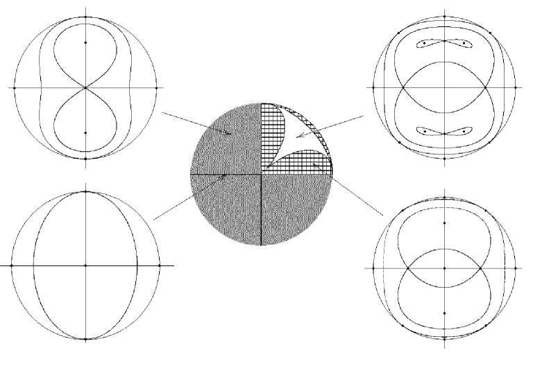
Figure 7: Regions of $\varepsilon_{i}$ corresponding to Types I - IV of the solutions to the auxiliary system. The white area indicates Type I solutions, the filled and the barred ones Type II and Type III. The lines dividing the Type I and Type II regions are subject to equations (II)

Figure 8: Comparison of solution to: A. the initial equations for geodesics; B. the averaged equation given by the auxiliary system.

The separatrix nets depend on values of the coefficients of the deformation $\varepsilon_{i}$, and generate regions I, II, III, IV in the $\varepsilon_{i}$ space.

It is important that the lines dividing the domains corresponding to types I and II, FIG.7, are given by the homogeneous equations

$$1. \quad\varepsilon_{1}\varepsilon_{2}-\varepsilon_{2}\varepsilon_{3}+\varepsilon_{3}\varepsilon_{1}=0$$

$$2. \quad\varepsilon_{1}\varepsilon_{2}+\varepsilon_{2}\varepsilon_{3}-\varepsilon_{3}\varepsilon_{1}=0$$

$$3. \quad-\varepsilon_{1}\varepsilon_{2}+\varepsilon_{2}\varepsilon_{3}+\varepsilon_{3}\varepsilon_{1}=0$$

The type of a graph corresponding to the solutions is completely determined by the numbers of foci and saddle points. The dependence of the conformations of the foci and the saddles on values of $\varepsilon_{i}$ is illustrated in FIG.7.

III Conclusion

The main instrument of the present investigation is the auxiliary Hamiltonian system, which can be considered as a reduction of the initial problem to a dynamical problem on specific configuration and phase spaces. Points of the new configuration space are geometrical objects, i.e great circles, of the configuration space, i.e. the standard sphere. Thus, we obtain a Hamiltonian system that describes the transformation of these objects. In a sense, the approach follows the classical method of Klein and Lie, Klein , of constructing a new space with objects of the given one. For the specific case of an ellipsoid close to the standard sphere our classification of orbits are in agreement with the classical results by Jacobi, J for geodesics on ellipsoid. We feel that our asymptotic approach is useful for the treatment of more general problems, for example the motion of rigid bodies, and intend to consider the problem in the subsequent paper. In analytical terms we study an asymptotic reduction of the system of equations for orbits on a deformed sphere to that of the top, but with the Hamiltonian of the fourth order. The simplification we get in this way, is substantial. Indeed, the initial Hamiltonian system could be non-integrable,whereas the auxiliary system is totally integrable and described by a graph that comprises vertices, which correspond to stationary solutions, or almost closed orbits, and edges, which can be visualized as orbits joining them, that is orbits which continuously approach more and more closely to coincidence with the closed ones.

References

• (1) E.T. Whittaker, A Treatise on the Analytical Dynamics, Chs. III, IV, XIII, Cambridge University Press, Cambridge (1927).
• (2) E.J.Routh, Dynamics of a System of Rigid Bodies, Ch.10, London - New York, Macmillan (1891).
• (3) R.W.Hamming, Numerical Methods for Scientists and Engineers, Ch.24, McGraw-Hill, New York (1962).
• (4) F.Klein, Vorlesungen über Höhere Geometrie, Ch.II, Springer Verlag, Berlin (1926).
• (5) C.G. Jacobi, Vorlesungen über Dynamik, Ch.28, URSS, Moscow (2004).