Asymptotic rate of quantum ergodicity in chaotic Euclidean billiards

Abstract

The Quantum Unique Ergodicity (QUE) conjecture of Rudnick-Sarnak is that every eigenfunction $\phi_{n}$ of the Laplacian on a manifold with uniformly-hyperbolic geodesic flow becomes equidistributed in the semiclassical limit (eigenvalue $E_{n}\to\infty$), that is, ‘strong scars’ are absent. We study numerically the rate of equidistribution for a uniformly-hyperbolic Sinai-type planar Euclidean billiard with Dirichlet boundary condition (the ‘drum problem’) at unprecedented high $E$ and statistical accuracy, via the matrix elements $\langle\phi_{n},\hat{A}\phi_{m}\rangle$ of a piecewise-constant test function $A$. By collecting $30000$ diagonal elements (up to level $n\approx 7\times 10^{5}$) we find that their variance decays with eigenvalue as a power $0.48\pm 0.01$, close to the estimate $1/2$ of Feingold-Peres (FP). This contrasts the results of existing studies, which have been limited to $E_{n}$ a factor $10^{2}$ smaller. We find strong evidence for QUE in this system. We also compare off-diagonal variance, as a function of distance from the diagonal, against FP at the highest accuracy ($0.7\%$) thus far in any chaotic system. We outline the efficient scaling method used to calculate eigenfunctions.

1 Introduction

The nature of the quantum (wave) mechanics of Hamiltonian systems whose classical counterparts are chaotic has been of long-standing interest, dating back to Einstein in 1917 (see [49] for a historical account). The field now called ‘quantum chaos’ is the study of such quantized systems in the short wavelength (semiclassical, $\hbar\rightarrow 0$ or high energy) limit, and has become a fruitful area of enquiry for both physicists (for reviews see [28, 30]) and mathematicians (see [43, 44, 63]) in recent decades. In contrast to those of integrable classical systems, eigenfunctions are irregular. A central issue, and the topic of this numerical study, is their behavior in the semiclassical limit.

We consider billiards, a paradigm problem in this field. A point particle is trapped inside a bounded planar domain $\Omega\subset\mathbb{R}^{2}$ and bounces elastically off the boundary $\Gamma=\partial\Omega$. Its phase space coordinate is $({\mathbf{r}},\theta)\in\Omega\times S^{1}$, with position ${\mathbf{r}}:=(x,y)$ and (momentum) direction $\theta$. The corresponding quantum-mechanical system is the spectral problem of the Laplacian in $\Omega$ with homogeneous local boundary conditions which we may (and will) take to be Dirichlet,

$$-\Delta\phi_{n} = E_{n}\phi_{n},$$ (1)

$$\phi_{n}(\Gamma) = 0.$$ (2)

Eigenfunctions $\phi_{n}$ are real-valued and normalized

$$\langle\phi_{n},\phi_{m}\rangle\;:=\;\int_{\Omega}\phi_{n}({\mathbf{r}})\phi_{m}({\mathbf{r}}){d{\mathbf{r}}}\;=\;\delta_{nm},$$ (3)

where ${d{\mathbf{r}}}:=dxdy$ is the usual area element, and the corresponding ‘energy’ (or frequency) eigenvalues are ordered $E_{1}<E_{2}\leq E_{3}\leq\cdots\infty$. We will also write $E_{j}=k_{j}^{2}$ where $k_{j}$ is the wavenumber. This Dirichlet eigenproblem [32], also known as the membrane or drum problem, has a rich 150-year history of applications to acoustics, electromagnetism, optics, vibrations, and quantum mechanics.

When the classical dynamics (flow) is ergodic it is well-known that almost all eigenfunctions are ‘quantum ergodic’, in the following sense.

Theorem 1 (Quantum Ergodicity Theorem (QET) [46, 55, 21, 62])

Let $\Omega\in\mathbb{R}^{2}$ be a 2D compact domain with piecewise smooth boundary whose classical flow is ergodic. Then for all $n$ except a subsequence of vanishing density,

$$\langle\phi_{n},\hat{A}\phi_{n}\rangle-\overline{A}\to 0\qquad\mbox{as}\;n\to\infty,$$ (4)

for all well-behaved functions $A:\Omega\to\mathbb{R}$.

The operator $\hat{A}$ is multiplication by $A$, a ‘test function’ whose spatial average is $\overline{A}:=\frac{1}{\operatorname{vol}(\Omega)}\int_{\Omega}A({\mathbf{r}})\,{d{\mathbf{r}}}$. The physical interpretation is that almost all quantum expectation values (diagonal matrix elements) of the observable $\hat{A}$ tend to their classical expectation $\overline{A}$, an example of the Correspondence Principle of quantum mechanics. Note the choice ‘almost all’ need not depend on $A$ [55]. Equivalently, almost all probability densities $|\phi_{j}|^{2}$ tend to the uniform function $\frac{1}{\operatorname{vol}(\Omega)}$, weakly in $L^{1}(\Omega)$ (see Fig. 2). The proof relies on the machinery of semiclassical analysis including Fourier Integral Operators (see [63, 36] and references within). In our context the ‘well-behaved’ requirement is, loosely speaking, that $A$ not be oscillatory on the (vanishing) wavelength scale $1/k_{j}$. (Formally $\hat{A}$ must be a zeroth-order pseudo-differential operator, a Weyl quantization of the principal symbol $A({\mathbf{r}})$). We investigate only multiplication operators, that is, no dependence on momentum, and, as we will see below, by further restricting to piecewise constant test functions we will exploit a huge numerical efficiency gain.

Our study is motivated by the fact that QET tells us nothing about the rate of convergence of $\langle\phi_{n},\hat{A}\phi_{n}\rangle$ or the density of the excluded subsequence, both of which are needed to understand the practical applicability of the QET in quantum or other eigenmode systems. We are interested in how the size of the deviation $\langle\phi_{n},\hat{A}\phi_{n}\rangle-\overline{A}$ varies with eigenvalue $E_{n}$. We define its ‘local variance’ (mean square value) at energy $E$ by

$$V_{A}(E):=\frac{1}{N_{L}(E)}\sum_{n:E_{n}\in[E,E+L(E)]}\left|\langle\phi_{n},\hat{A}\phi_{n}\rangle-\overline{A}\right|^{2},$$ (5)

where $N_{L}(E):=N(E+L(E))-N(E)$ and the level counting function is

$$N(E):=\#\{n:E_{n}\leq E\}$$ (6)

Here we envisage an energy window width $L(E)=O(E^{1/2})$, that is, a wavenumber window of width $O(1)$: this contains $O(E^{1/2})$ eigenvalues by Weyl’s Law [28, 63]. For practical reasons (Section 4.1) we will in fact use other $L(E)$ widths which nevertheless contain many ($\approx 10^{3}$) eigenvalues. We will test the following asymptotic form for the variance.

Conjecture 1 (Power-law diagonal variance)

For ergodic flow, as $E\to\infty$, there is the asymptotic form, for some $a$ and $\gamma$,

$$V_{A}(E)\sim aE^{-\gamma}.$$ (7)

A random-wave model for eigenfunctions (Section 2.1) predicts $\gamma=1/2$ and a certain prefactor $a_{\mbox{\tiny RW}}$. We will also test a more elaborate heuristic from the physics literature (Section 2.2) which predicts $\gamma=1/2$ and the following different prefactor.

Conjecture 2 (Feingold-Peres diagonal variance [26, 24])

For ergodic flow with no symmetries other than time-reversal,

$$V_{A}(E)\sim\frac{g\tilde{C}_{A}(0)}{\operatorname{vol}(\Omega)}E^{-1/2}$$ (8)

where the symmetry factor is $g=2$.

Here the prefactor $\tilde{C}_{A}(\omega)$ is the power spectral density (also known as classical variance [44], spectral measure [60, 63], or fluctuations intensity [20]),

$$\tilde{C}_{A}(\omega)\;:=\;\int_{-\infty}^{\infty}C_{A}(\tau)e^{i\omega\tau}d\tau,$$ (9)

the time autocorrelation of $A$ being

$$C_{A}(\tau):=\lim_{T\to\infty}\frac{1}{T}\int_{0}^{T}\!A({\mathbf{r}}(t))A({\mathbf{r}}(t+\tau))\,dt,$$ (10)

where ${\mathbf{r}}(t)$ is any uniformly-distributed (ergodic) trajectory.

Remark 1.1

In the physics literature much stronger conjectures are often discussed, such as individual matrix elements $\langle\phi_{n},\hat{A}\phi_{n}\rangle$ being pseudo-randomly distributed with variance given as above. We present evidence for this in Section 4.2. At the other extreme, proven theorems (and some numerical work [5]) often involve sums of the form $S_{p}(E;A):=N(E)^{-1}\sum_{j:E_{j}\leq E}\left|\langle\phi_{j},\hat{A}\phi_{j}\rangle-\overline{A}\right|^{p}$. Note that asymptotic decay $S_{p}(E;A)\sim bE^{-p\gamma/2}$ is equivalent to Conjecture 7. However we will study $V_{A}(E)$ rather than $S_{p}(E;A)$ for the following important practical reasons:

1. Narrow spectral windows are needed rather than the complete spectrum, allowing much higher eigenvalues to be included in the statistics.

2. Asymptotic behavior will emerge sooner since data at high $E_{n}$ are not averaged with that from the lower part of the spectrum.

About 10% agreement with Conjecture 2  has been shown in the quantum bakers map [24], and rough agreement with $\gamma=1/2$ has been found in hyperbolic polygons [2]. For general ergodic flow, proven bounds on the power-law rate $\gamma$ in Conjecture 7  are quite wide: Zelditch [58] has shown that $S_{p}(E;A)=O((\log E)^{-p/2})$, implying $\gamma>0$, and shown [59] that for generic $A$ (more precisely, one with nonzero mean sub-principal symbol), $\gamma\leq 1$.

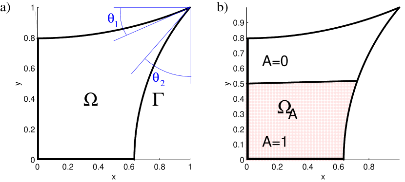
Figure 1: Billiard and test function used in this study. a) Quarter generalized Sinai billiard formed by two circular arcs which meet at $(1,1)$ at angles $\theta_{1}=0.4$ to the horizontal and $\theta_{2}=0.7$ to the vertical. The straight sections lie on the axes and meet the arcs at right angles. b) Piecewise-constant $A({\mathbf{r}})$ which takes the value $1$ inside the region $\Omega_{A}$ and zero elsewhere. $\partial\Omega_{A}\setminus\Gamma$ is a straight line which does not meet either wall at right angles.

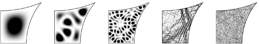
Figure 2: Illustration of spatial equidistribution of $|\phi_{n}|^{2}$ (shown as density plots; larger values are darker) with increasing eigenvalue: $n^{th}$ Dirichlet eigenfunction for mode numbers $n=1,10,100,1000$ and $n\approx 50000$.

There are special ‘arithmetic’ manifolds with ergodic flow for which powerful number-theoretic tools [42, 44] allow much more to be proven. For the quotient manifold ${\mathbf{H}}^{2}/SL(2,\mathbb{Z})$ Luo and Sarnak [35] recently showed $S_{2}(E;A)\sim B(A)E^{-1/2}$, where the prefactor is a quadratic form $B(\cdot)$ diagonalized by the eigenfunctions themselves. It takes the value $B(\phi_{n})=\tilde{C}(0)L({\textstyle\frac{1}{2}},\phi_{n})$, where $L(\cdot,\cdot)$ is an L-function [44]. Thus the power law appearing in Conjecture 2  holds but the prefactor differs from $g=2$. This is hardly surprising; Sarnak [44] notes that a simple reflection symmetry is enough to cause $g=0$. Arithmetic systems are very special and have many symmetries: all periodic orbits possess a single Lyapunov exponent, and eigenvalue spacing statistics are unusual for ergodic systems [16]. This makes the study of a planar Euclidean billiard system without symmetry (where Lyapunov exponents differ), for which no number-theoretic analytic tools exist, particularly interesting. We choose such a generic billiard (with hyperbolic, i.e. Anosov, flow [47]) for our numerical experiments (see Fig. 1). Numerical tests of Conjecture 7  (in the form of $S_{1}(E;A)$, see Remark 1.1) exist for low eigenvalues ($n<6000$) in the Anosov cardioid billiard [5]: various powers were found in the range $\gamma=0.37$ to 0.5, and up to 20% deviations from the prefactor in Conjecture 2.

We address two other questions, the first regarding the excluded subsequence in Theorem 1, the second regarding off-diagonal matrix elements.

Conjecture 3 (Quantum Unique Ergodicity (QUE) [41])

There is no excluded subsequence in Thm. 1.

‘Unique’ refers to the existence of only one ‘quantum limit’ (any measure to which $|\phi_{n}|^{2}$ tends weakly). Made in the context of general negatively-curved manifolds, this conjecture has remarkably been proved for arithmetic manifolds [34]. In contrast, QUE has been proven not to hold for certain-dimensional quantizations of Arnold’s cat map [25]. This begs the question: for which ergodic billiards, if any, does this conjecture hold? For instance there is strong evidence [50, 4] (but no proof [23]) that a sequence of ‘bouncing ball’ modes (eigenfunctions concentrated on cylindrical or neutrally stable orbits which occupy zero measure in phase space) persists to arbitrarily high eigenvalues in ergodic billiards such as Bunimovich’s stadium. Since such modes are not spatially uniform, the conjecture would not hold for this shape. There are also more subtle nonuniformity effects: in the physics community enhancements of $|\phi_{n}|^{2}$, dubbed ‘scars’ by Heller [29, 30], are known to exist along isolated unstable periodic orbits, and there has been a long-standing debate as to whether these may prevent QUE. In Section 4.4 we discuss how our results relate to scarring.

Finally we consider the size of off-diagonal matrix elements $\langle\phi_{n},\hat{A}\phi_{m}\rangle$. Define $\Delta_{k}(E):=2\pi/[E^{1/2}\operatorname{vol}(\Omega)]$ as the mean level spacing (in wavenumber).

Conjecture 4 (Feingold-Peres off-diagonal variance [26, 54])

Fix $\omega\in\mathbb{R}$. Then for ergodic flow, as $E\to\infty$ there is the asymptotic result,

$$V_{A}(E;\omega)\;:=\;\frac{\Delta_{k}(E)}{2\epsilon(E)\,N_{L}(E)}\sum_{\begin{subarray}{c}m,n:E_{n}\in[E,E+L(E)]\\ |k_{m}-k_{n}-\omega|\leq\epsilon(E)\end{subarray}}\!\!\!|\langle\phi_{n},\hat{A}\phi_{m}\rangle|^{2}\;\sim\;\frac{\tilde{C}_{A}(\omega)}{\operatorname{vol}(\Omega)}E^{-1/2}$$ (11)

where $0<\epsilon(E)=O(E^{-1/4})$.

$V_{A}(E;\omega)$ measures the mean off-diagonal quantum variance a ‘distance’ (in wavenumber units) $\omega$ from the diagonal, which is thus given by classical variance at frequency $\omega$ (see Section 2.2 for a heuristic argument). As above, the choice $L(E)=O(E^{1/2})$ is envisaged. The rate at which the wavenumber window $\epsilon(E)$ vanishes includes a growing number $O(E^{1/4})$ of modes. The result (with equivalent choices of $L(E)$ and $\epsilon(E)$) has been proved for Schrödinger operators with smooth confining potential using coherent states [22]. Conjecture 4 is a stronger version of the spectral measure theorem [60, 51]

$$\lim_{E\to\infty}\frac{1}{N(E)}\sum_{\begin{subarray}{c}m,n:E_{n}\in[0,E]\\ \alpha<k_{m}-k_{n}<\beta\end{subarray}}\!\!\!|\langle\phi_{n},\hat{A}\phi_{m}\rangle|^{2}\;=\;\int_{\alpha}^{\beta}\frac{\tilde{C}_{A}(\omega)}{2\pi}d\omega,$$ (12)

which holds for $\alpha<\beta$ independent of ergodicity. It is known $V_{A}(E;\omega)$ vanishes for ergodic weak-mixing flows (weak-mixing ensures $\tilde{C}_{A}(\omega)$ is a bounded function), but without any proven rate [56]. The most accurate previous numerical test of Conjecture 4 is the 10% agreement found for billiards with $\hat{A}$ a singular boundary operator [8]. Other tests have included the quartic oscillator [3], bakers map [18], and limaçon billiard [39].

Existing numerical studies of all the above conjectures share the features of low and poorly-quantified accuracy (i.e. lack of statistical rigor in the tests), and relatively low mode numbers ($n\sim 10^{3}$ to $10^{4}$). In this work we remedy both these flaws by performing a large-scale study using non-standard cutting-edge numerical techniques which excel at very high eigenvalues. In Section 2.2 we review heuristic arguments for Conjectures 7, 2 and 4. Then in Section 3 (which refer to the three Appendices) we outline numerical methods; we emphasize there are several innovations. However the reader interested in the results on the four Conjectures, and discussion, may skip directly to Section 4. We summarize our conclusions in Section 5.

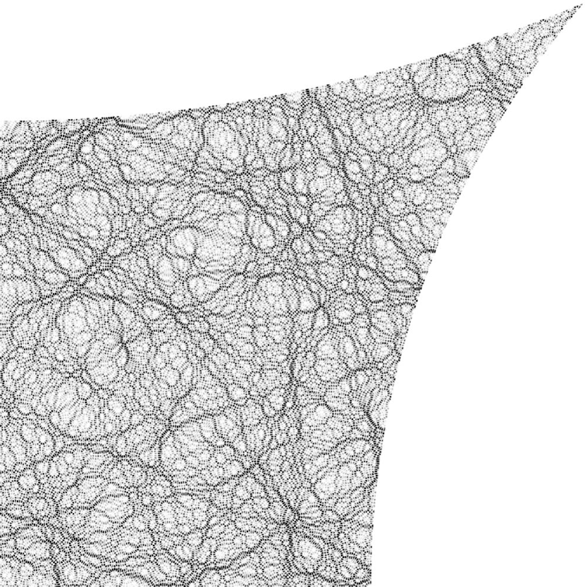
Figure 3: Density plot of $|\phi_{n}|^{2}$ for an eigenfunction with $k_{n}=999.90598\cdots$, that is, $E_{n}\approx 10^{6}$, and level number $n\approx 5\times 10^{4}$. There are about 225 wavelengths across the diagonal.

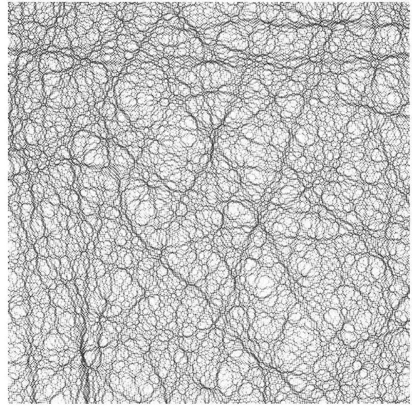
Figure 4: Density plot of one sample from the ensemble of random plane waves with the same wavenumber magnitude $|{\mathbf{k}}|=k$ and mean intensity as the eigenfunction in Fig. 3, shown in a square region of space. (Note there are no boundary conditions imposed). The ‘stringy’ structures visible to the eye are a feature of the constant wavevector magnitude; they disappear if a finite range of $k$ is included [30].

2 Heuristic arguments for ergodicity rate

Here we review some arguments for Conjectures 7, 2 and 4 from the physics literature. We feel these are appropriate since quantum chaos is somewhat of a cross-over area between mathematics and physics.

2.1 Random wave model

Berry [12] put forward the conjecture that chaotic eigenfunctions should look locally like a superposition of plane waves of fixed energy $E$, traveling in all directions, with random amplitudes and phases (compare Figs. 3 and 4). We will show (following [24]) that this model satisfies Conjecture 7  with certain $\gamma$ and $a$. We note that Zelditch has more rigorously considered models of random orthonormal bases on manifolds, and shown that they possess similar ergodicity properties to quantum chaotic eigenfunctions [57, 61].

Using the notation $\langle\,\cdot\,\rangle$ to denote averaging over the ensemble of plane wave coefficients, the two-point correlation of a random-wave field is [12]

$$\langle\phi({\mathbf{r}}_{1})\phi({\mathbf{r}}_{2})\rangle=\frac{1}{\operatorname{vol}(\Omega)}J_{0}(k|{\mathbf{r}}_{1}-{\mathbf{r}}_{2}|),$$ (13)

where we use the normalization $\operatorname{vol}(\Omega)\langle\phi^{2}\rangle=1$ appropriate to the billiard area. This applies to both real (time-reversal symmetric) and complex (non time-reversal symmetric) waves; from now we stick to the real case. Because the model is a statistical one, it is meaningful to speak of the variance of a particular matrix element within the ensemble, namely $\mbox{var}(A_{nm})$ where we use $A_{nm}:=\langle\phi_{n},\hat{A}\phi_{m}\rangle$. A simple calculation using (13) and Wick’s theorem for Gaussian random variables gives

$$\langle\phi_{n}({\mathbf{r}}_{1})\phi_{m}({\mathbf{r}}_{1})\phi_{n}({\mathbf{r}}_{2})\phi_{m}({\mathbf{r}}_{2})\rangle=\frac{1}{\operatorname{vol}(\Omega)^{2}}\left[\delta_{nm}+g_{nm}J_{0}^{2}(k|{\mathbf{r}}_{1}-{\mathbf{r}}_{2}|)\right]$$ (14)

where

$$g_{nm}:=\left\{\begin{array}[]{ll}g,&n=m,\\ 1,&n\neq m.\end{array}\right.$$ (15)

Here the symmetry factor is $g=2$; we will shortly see it gives the ratio of diagonal to off-diagonal variance. A key assumption made was that $\phi_{n}$ and $\phi_{m}$ are statistically independent members of the ensemble when $n\neq m$, a natural one in the context of random matrix theory (RMT) ($g=2$ for time-reversal symmetry is a standard result in the Gaussian Orthogonal Ensemble [17]). The independence assumption, like the random wave model itself, remains a heuristic one, albeit one with numerical support. Clearly orthogonality (3) dictates that, when considered as functions over all of $\Omega$, $\phi_{n}$ and $\phi_{m}$ cannot be independent! (As was mentioned there are improved models which take this into account [61]). An intuitive argument can be made if a restriction to a small subregion of $\Omega$ is made: the eigenfunctions behave like random orthogonal vectors, and projections of such vectors onto a much smaller-dimensional subspace become approximately independent.

Now we use (14) to evaluate the variance diagonal and off-diagonal matrix elements, writing the variance as the mean square minus the square mean,

$$\mbox{var}(A_{nm}) = \langle\left|\int_{\Omega}\phi_{n}({\mathbf{r}})\phi_{m}({\mathbf{r}})A({\mathbf{r}}){d{\mathbf{r}}}\right|^{2}\rangle\;-\;\langle A_{nm}\rangle^{2}$$ (16)

$$= \frac{g_{nm}}{\operatorname{vol}(\Omega)^{2}}\int_{\Omega}\int_{\Omega}J_{0}(k_{n}|{\mathbf{r}}_{1}-{\mathbf{r}}_{2}|)J_{0}(k_{m}|{\mathbf{r}}_{1}-{\mathbf{r}}_{2}|)d{\mathbf{r}}_{1}d{\mathbf{r}}_{2}$$

$$\approx \frac{g_{nm}}{\pi\operatorname{vol}(\Omega)}E^{-1/2}\int_{\Omega}\int_{\Omega}\frac{A({\mathbf{r}}_{1})A({\mathbf{r}}_{2})}{|{\mathbf{r}}_{1}-{\mathbf{r}}_{2}|}d{\mathbf{r}}_{1}d{\mathbf{r}}_{2},$$

where we used $\langle A_{nm}\rangle=\delta_{nm}\overline{A}$. In the final step two approximations have been made: i) $L|k_{n}-k_{m}|\ll 1$ where $L$ is the largest spatial scale of $A({\mathbf{r}})$, meaning that the two Bessel functions always remain in phase so can be set equal, and ii) the asymptotic form $J_{0}(x)\sim(2/\pi x)^{1/2}\cos(x-\pi/4)$ was used, and $\cos^{2}$ replaced by its average value ${\textstyle\frac{1}{2}}$, giving a semiclassical expression valid when $kl\gg 1$, where $l$ is the smallest relevant spatial scale in $A({\mathbf{r}})$. Considering the diagonal and off-diagonal cases, (16) implies

$$\mbox{var}(A_{nn})=g\,\mbox{var}(A_{nm})$$ (17)

in a region $n\approx m$ close enough to the diagonal. The diagonal case of (16) gives the power law $\gamma=1/2$,

$$V_{A}(E)\;\approx\;a_{\mbox{\tiny RW}}E^{-1/2},$$ (18)

where the prefactor takes the form of a Coulomb interaction energy of the ‘charge density’ $A({\mathbf{r}})$,

$$a_{\mbox{\tiny RW}}=\frac{g}{\pi\operatorname{vol}(\Omega)}\iint\frac{A({\mathbf{r}}_{1})A({\mathbf{r}}_{2})}{|{\mathbf{r}}_{1}-{\mathbf{r}}_{2}|}d{\mathbf{r}}_{1}d{\mathbf{r}}_{2}.$$ (19)

Note that this model takes no account of the billiard shape or boundary conditions.

2.2 Classical autocorrelation argument (FP)

Feingold and Peres [26] were the first to derive a semiclassical expression for diagonal variance in chaotic systems. There are two steps:

1. relating off-diagonal variance to $\tilde{C}_{A}(\omega)$ the power spectral density, yielding Conjecture 4, then

2. relating diagonal variance to off-diagonal variance close to the diagonal, yielding Conjecture 2.

Step (i): Our presentation is loosely based on Cohen [20]; we emphasize that this is not a mathematical proof, rather one form of a heuristic common in physics literature (cf. [54, 39, 31, 24]). The autocorrelation (10) of the ‘signal’ $A({\mathbf{r}}(t))$ associated with a uniformly-distributed ergodic unit-speed trajectory ${\mathbf{r}}(t)$ is $C_{A}(\tau)=\overline{A(0)A(\tau)}$, where the ergodic theorem was used to rewrite the time average as an average over initial phase space locations $({\mathbf{r}}_{0},\theta_{0})$. Fixing $\tau$ gives the function of phase space ${\cal A}({\mathbf{r}}_{0},\theta_{0}):=A(0)A(\tau)$. Applying QET to this function ${\cal A}$, gives as $E\to\infty$,

$$N_{L}(E)^{-1}\!\!\!\sum_{n:E_{n}\in[E,E+L(E)]}\langle\phi_{n},\hat{A}(0)\hat{A}(\tau)\phi_{n}\rangle\;\sim\;C_{A}(\tau),$$ (20)

where $\hat{A}(t)$ is the quantization of $A$, shifted in time (according to the Heisenberg picture of quantum mechanics). A window $L(E)=O(E^{1/2})$ is sufficient for validity of QET [63]. Assuming a wave dispersion relation $\omega=k$ the operator $\hat{A}(t)$ is expressed in the eigenfunction basis,

$$\langle\phi_{n},\hat{A}(t)\phi_{m}\rangle\;=\;A_{nm}e^{-i(k_{m}-k_{n})t}.$$ (21)

Using this and inserting a sum over projections onto all eigenfunctions into (20) gives

$$N_{L}(E)^{-1}\!\!\!\sum_{n:E_{n}\in[E,E+L(E)]}\,\sum_{m=1}^{\infty}|A_{nm}|^{2}e^{-i(k_{m}-k_{n})\tau}\;\sim\;C_{A}(\tau).$$ (22)

Taking the inverse Fourier transform of the definition in (11), recognising $\lim_{\epsilon\to 0}(2\epsilon)^{-1}1_{[-\epsilon,\epsilon]}$ as the Dirac delta function, and using (22), gives

$$\frac{1}{2\pi}\int e^{-i\omega\tau}V_{A}(E;\omega)\,d\omega\;\sim\;\frac{\Delta_{k}(E)}{2\pi}C_{A}(\tau).$$ (23)

Finally, taking a Fourier transform and substituting $\Delta_{k}(E)$ gives Conjecture 4.

Step (ii): To approach the diagonal we take the limit $\omega\to 0$; here $\tilde{C}_{A}(\omega)$ is well-defined and bounded since the flow is weak-mixing [60]. The expectation that diagonal variance should exceed off-diagonal variance by the time-reversal invariance symmetry factor (17) with $g=2$ gives Conjecture 2. Feingold-Peres [26] justify this by considering $\phi_{\pm}:=(\phi_{n}\pm\phi_{m})/\sqrt{2}$ for eigenfunctions $\phi_{n}$ and $\phi_{m}$ with sufficiently small $E_{n}-E_{m}$. Matrix elements are then $\langle\phi_{+},\hat{A}\phi_{-}\rangle=(A_{nn}-A_{mm})/2$, where $A=A^{*}$ was used; these are expected (by rotational invariance) to have the same variance as $A_{mn}$. Treating these quantities as independent statistical variables, taking variances, and recognising that mean values $\overline{A}$ cancel on the right, gives $\mbox{var}(A_{mn})=\mbox{var}(A_{+-})=\mbox{var}(A_{nn})/2$, that is, $g=2$. Although this was not discussed by FP, the system must be assumed to be without further symmetry, or other values of $g$ may result.

Finally, the physical significance of the correlation functions used above should be noted: the right-hand side of (11) is proportional to dissipation (heating) rate in a classical system driven at frequency $\omega$ with the forcing function $A$, and the left-hand side to quantum dissipation rate under equivalent forcing (with $\hat{A}$) within linear response theory (for reviews see [20, 9, 7]).

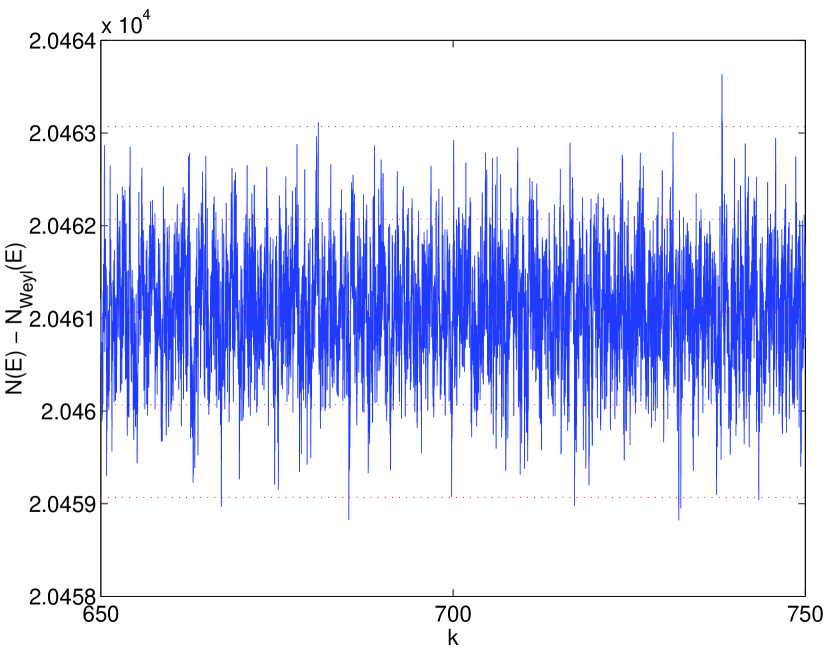
Figure 5: Demonstration that none of the 6812 modes are missing in the wavenumber window $k_{n}\in[650,750]$. The level counting function (6) is plotted after the first two Weyl terms $N_{\mbox{\tiny Weyl}}(E)=(\operatorname{vol}(\Omega)/4\pi)E-(|\Gamma|/4\pi)\sqrt{E}$ have been subtracted. The horizontal axis shows wavenumber $k=E^{1/2}$. Spectral rigidity ensures that a single missing or extra mode can be detected [28]; this would be visible as a permanent jump of size 1 (the gap between the dotted horizontal lines). No such jump occurs.

3 Computing quantum matrix elements

Our nonsymmetric billiard $\Omega$ is shown in Fig. 1a and defined in the caption. Its classical autocorrelation has already been studied [9]. In App. A we present the method used to compute $\tilde{C}_{A}(\omega)$ to an accuracy of a fraction of a percent (this is much less time-consuming than the following quantum computations). Note that since two walls are the coordinate axes it is a desymmetrized version of a billiard of four times the area formed by unfolding reflections in $x$ and $y$. Desired eigenfunctions are then the subset of odd-odd symmetric eigenfunctions of the unfolded billiard, a fact that enables use of a smaller symmetrized basis set (hence higher eigenvalues), and a reduction of the effective boundary to $\Gamma_{\mbox{\tiny desym}}$, the part of $\Gamma$ which excludes the symmetry lines (axes), accelerating the quantum calculation by a factor of about 4 [7].

We chose the test function $A({\mathbf{r}})$ to be the characteristic function of the subdomain $\Omega_{A}$ shown in Fig. 1b which falls one side of the straight line $\partial\Omega_{A}\setminus\Gamma$. Our choice of the shape of $\Omega_{A}$ was informed by the issue of boundary effects raised by Bäcker et al. [5], the main point being that within a boundary layer of order a wavelength, there are Gibbs-type phenomena associated with spectral projections, and by choosing a large angle of intersection of the line with $\Gamma$ their contribution is minimized. Our classical mean is $\overline{A}=\operatorname{vol}(\Omega_{A})/\operatorname{vol}(\Omega)\approx 0.55000$. Matrix elements $\langle\phi_{n},\hat{A}\phi_{m}\rangle=\langle\phi_{n},\phi_{m}\rangle_{\Omega_{A}}$ are computed using integrals of eigenfunctions in an efficent manner described shortly.

Eigenfunctions and eigenvalues were found with the ‘scaling method’ [53, 7], outlined further in App. B. This is a little-known basis approximation method, a variant of the Method of Particular Solutions [14, 32], which uses collocation on $\Gamma_{\mbox{\tiny desym}}$ to extract all eigenvalues lying in an energy window $E_{n}\in[E,E+L(E)]$, where $L(E)$ is $O(E^{1/2})$. The equivalent wavenumber window is $O(1)$. The spectrum in larger intervals can then be found by collecting from sufficiently many windows. We are certain that all modes and no duplicates have been found in the desired intervals, as demonstrated by comparing the counting function against Weyl’s law in Fig. 5. At energy $E$ (wavenumber $k$) the required basis size $N=O({N_{\mbox{\tiny sc}}})$, the ‘semiclassical basis size’, is

$${N_{\mbox{\tiny sc}}}\;:=\;\frac{k|\Gamma_{\mbox{\tiny desym}}|}{\pi},$$ (24)

where $|\Gamma_{\mbox{\tiny desym}}|$ indicates the desymmetrized perimeter. Rather than evaluating $\phi_{n}$ at a set of points covering all of $\Omega$, which would be very expensive, only basis coefficients of $\phi_{n}$ are computed, from which $\phi_{n}({\mathbf{r}})$ can be later computed at any desired location. Computational effort is $O(N^{2})=O(E)$ per mode, assuming $O(N^{3})$ theoretical effort for dense matrix diagonalization (in fact because of memeory limitations, for large $N$ it was not this favorable). Because of the simultaneous computation of many modes, the scaling method is faster by $O(N)$ than any other known method (see overview in [32, 7]) such as boundary integral equations [6]. We needed $N\approx 3500$ at the largest wavenumber reached ($k_{n}\approx 4000$, at $n\approx 7\times 10^{5}$) for the billiard under study; in this case the resulting efficiency gain is roughly a factor of a thousand! Similar efficiency gains have been reported in other studies of the Dirichlet eigenproblem at extremely high energy in both 2D [53, 52, 19] and 3D [40]. Only a couple of studies in billiards have computed eigenfunctions at greater $n$, and they invariably involved shapes without corners (for example [19]). Note that in App. B we outline the basis set innovation that allows us to handle non-convex shapes and (non-reentrant) corners effectively. Despite its success the scaling method has not yet been analysed in a rigorous fashion [11].

Once a large set of eigenfunctions (in the form of their basis coefficients) have been found, such as the example plotted in Fig. 3, matrix elements may be efficiently computed as we now show. The following is proved in App. C.

Lemma 3.1

Fix $E>0$ and let $-\Delta u=Eu$ and $-\Delta v=Ev$ hold in a Lipschitz domain $\Omega_{A}\in\mathbb{R}^{2}$. Let ${\mathbf{n}}$ be the outwards unit normal vector at boundary location ${\mathbf{r}}\in\partial\Omega_{A}$ (${\mathbf{r}}$ is measured relative to some fixed origin), and $ds$ be surface measure. Then

$$\langle u,v\rangle_{\Omega_{A}}=\frac{1}{2E}\oint_{\partial\Omega_{A}}\!\!({\mathbf{r}}\cdot{\mathbf{n}})(Euv-\nabla u\cdot\nabla v)+({\mathbf{r}}\cdot\nabla u)({\mathbf{n}}\cdot\nabla v)+({\mathbf{r}}\cdot\nabla v)({\mathbf{n}}\cdot\nabla u)\;ds.$$

This boundary integral identity, with the substitution $u=v=\phi_{n}$, allows diagonal matrix elements to be calculated using 1D rather than 2D numerical integration. Since typically 10 quadrature points per wavelength are needed for integration, and our system is up to hundreds of wavelengths in size, this is an enormous efficiency gain of order $O(N)$ or $10^{3}$. Note that the boundary integrand is nonzero only on the line $\partial\Omega_{A}\setminus\Gamma$. Off-diagonal matrix elements are found via the following identity which is a simple consequence of the Divergence Theorem.

Lemma 3.2

Let $-\Delta u=E_{u}u$ and $-\Delta v=E_{v}v$ hold with $E_{u}\neq E_{v}$, and other conditions as above, then

$$\langle u,v\rangle_{\Omega_{A}}\;=\;\frac{1}{E_{u}-E_{v}}\oint_{\partial\Omega_{A}}\!(u{\mathbf{n}}\cdot\nabla v-v{\mathbf{n}}\cdot\nabla u)\;ds.$$

Again we use $u=\phi_{n}$, $E_{u}=E_{n}$, $v=\phi_{m}$, $E_{v}=E_{m}$, and the integrand is nonzero only on $\partial\Omega_{A}\setminus\Gamma$.

Thus values and first derivatives of eigenfunctions on boundaries alone are sufficient to evaluate all matrix elements. Note the eigenfunctions need never be evaluated in the interior of $\Omega_{A}$. For the boundary integrals, $O(N)$ quadrature points are needed, and at each point $O(N)$ basis evaluations are needed to find $\phi_{n}$ and its gradient, giving $O(N^{2})$ effort per eigenfunction, the same effort required to find modes by the scaling method. The calculations reported in this work took only a few CPU-days (1GHz Pentium III equivalent, 1–2 GB RAM) in total. The effort is divided roughly equally between evaluating basis (Bessel) functions and their gradients at the quadrature points, and dense matrix diagonalization.

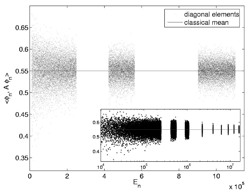
Figure 6: Scatter plot of diagonal matrix elements $\langle\phi_{n},\hat{A}\phi_{n}\rangle$ plotted against energy eigenvalue $E_{n}$. The gaps are due to the fact that only certain windows on the $E$ axis have been computed; within each window all eigenvalues are found. The windows shown in the main plot correspond to wavenumbers $k_{n}\in[100,500]$, $k_{n}\in[650,750]$ and $k_{n}\in[950,1050]$, giving a total of 28171 modes. The classical mean $\overline{A}$ is shown as a horizontal line. The inset shows the complete energy range (including the 2718 higher modes not shown in the main plot) on a log scale, with larger points to make extreme values evident.

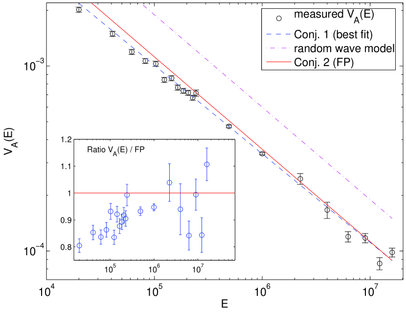
Figure 7: Log-log plot of diagonal variance $V_{A}(E)$ (with $\pm 1\sigma$ errorbars) as a function of energy $E$. The smallest errorbar is about 1.4% (at $E\approx 10^{6}$). For Conjecture 7  the best-fit power law $(\gamma_{\mbox{\tiny BF}},a_{\mbox{\tiny BF}})$ is shown as the dashed line. The random wave prediction (18) and (19) is the dash-dotted line. Conjecture 2  (FP) is shown as a solid line, and the ratio of $V_{A}(E)$ to this prediction is shown in the inset.

	Best-fit	Random wave	Feingold-Peres
	$a_{\mbox{\tiny BF}}^{(1/2)}$	$a_{\mbox{\tiny RW}}$	$a_{\mbox{\tiny FP}}$
prefactor	$0.334\pm 0.003$	$0.5995\pm 0.001$	$0.3550\pm 0.0004$
deviation from $a_{\mbox{\tiny BF}}^{(1/2)}$	—	$79\pm 1\%$	$6.5\pm 0.9\%$

Table 1: Comparison of best-fit prefactor $a$ in Conjecture 7, assuming fixed power $\gamma=1/2$, against the random wave prediction (19), and the Feingold-Peres prefactor $a_{\mbox{\tiny FP}}:=2\tilde{C}_{A}(0)/\operatorname{vol}(\Omega)$ of Conjecture 2.

4 Results and discussion

4.1 Diagonal variance (Conjectures 7 and 2)

Fig. 6 shows a sample of raw diagonal matrix element data, using only eigenvalues in certain intervals, up to $k\approx 10^{3}$ ($E\approx 10^{6}$). From this we chose a sequence of $E$ values and computed $V_{A}(E)$ at each. Computing matrix elements at high eigenvalues is very costly, so it would be inefficient and impractical numerically to grow the interval width as $L(E)=cE^{1/2}$ for some constant $c$. This would either involve ignoring, or breaking in to very short intervals (which would introduce large relative fluctuations) low eigenvalue data which is cheap to collect, or requiring vast numbers of modes at high eigenvalue which is too expensive. Rather, we chose a convenient value of $L(E)$ at each $E$ that allowed a large number of modes $M$ to be summed at that $E$, while still allowing access to the highest $E$ values possible ($E\approx 1.6\times 10^{7}$). Specifically, we split the lowest interval shown ($k_{n}\in[100,500]$) into intervals containing about $10^{3}$ modes each, kept the two other intervals shown intact (each containing an extremely large number of order $10^{4}$), and at the higher eigenvalues (see inset of Fig. 6) chose intervals containing 200–700 modes each.

One may ask how the $V_{A}(E)$ values obtained this way would differ from those obtained using a strictly growing $L(E)=cE^{1/2}$. To indicate the flutuations in $V_{A}(E)$ expected from summing over a finite sample size $M$, we included an errorbar of relative size $\sqrt{2/M}$. For example $M=20000$ corresponds to 1% errorbar (illustrating that high statistical accuracy is computationally intensive). This model does assume that deviations $|\langle\phi_{n},\hat{A}\phi_{n}\rangle-\overline{A}|$ are roughly statistically independent, an assumption motivated by RMT [17]. We find (see inset of Fig. 7) that observed fluctuations in $V_{A}(E)$ fit this assumption well, so that even if correlations are present they do not affect our conclusions much. Thus if longer sums were indeed computed using $L(E)=cE^{1/2}$, it is likely that their values would lie within the errorbars shown. The resulting local variance is presented in Fig. 7. A power-law dependence is immediately clear. We fitted the power-law model of Conjecture 7, obtaining a best-fit power

$$\gamma_{\mbox{\tiny BF}}\;=\;0.479\pm 0.009,$$ (25)

differing by only $4\pm 2\%$ from the random-wave model and Conjecture 2  value $\gamma=1/2$. For this fit we used weighted least-squares, weighted using the numbers of modes $M$ (equivalently, errorbars) for each interval. In a standard maximum-likelihood framework [48] we marginalized over $a$ to obtain the quoted errorbar in $\gamma$. We also excluded a low-eigenvalue regime found to be non-asymptotic, taking only data with $E>E_{\mbox{\tiny min}}=1.6\times 10^{5}$. (Our criterion here was that if any lower $E_{\mbox{\tiny min}}$ was used, the fitted $\gamma_{\mbox{\tiny BF}}$ was found to dependent on $E_{\mbox{\tiny min}}$). This best-fit power-law is shown in Fig. 7; the data are completely consistent with Conjecture 7.

The random wave model and Conjecture 2  both involve the power $\gamma=1/2$. Therefore to test their validity the power was held fixed at this value while fitting only for the prefactor $a$, with results given in Table 1. Notice that the random wave model is a poor predictor; this might be expected since this model takes no account of the boundary conditions, yet the support of the test function $A$ extends to the boundary and covers a large fraction of the volume. Intuitively speaking, images (boundary reflections) of $A$ are not being taken into account, and evidently this is a large effect.

The prefactor (which is dominated by the large numbers of modes at $E\approx 10^{6}$) is overestimated by Conjecture 2  by only 6.5%, however this is statistically significant (a $7\sigma$ effect). The systematic deviation is highlighted in the inset of Fig. 7, where it appears that the deviation decreases with $E$. This is especially clear for $E\approx 10^{6}$ or below, and asymptotic agreement with Conjecture 2 is not inconsistent with the large scatter of the highest six datapoints (since they have larger errorbars). If Conjecture 2  is correct, our results show that convergence must be alarmingly slow. This may explain why previous numerical billiard studies [2, 5] found various power-laws and prefactors differing by up to 20% from Conjecture 2, depending on choice of billiard and $A$: they had failed to reach the asymptotic regime. We achieve this with mode numbers 100 times higher than these studies. We might model slow convergence to Conjecture 2  by a correction, for example,

$$V_{A}(E)\;\sim\;\frac{g\tilde{C}_{A}(0)}{\operatorname{vol}(\Omega)}E^{-1/2}\left(1-bE^{-\beta}+o(E^{-\beta})\right),$$ (26)

with $\beta$ sufficiently small, and $b$ sufficiently large. Our current data do not allow a meaningful fit for $\beta$ and $b$, however, they suggest $0.25\leq\beta\leq 0.5$, and that $b$ is several times greater than 1. We note that in the physics literature periodic-orbit corrections to Conjecture 2 derived by Wilkinson [54] were later claimed by Prosen not to contribute at this order [39]. Clearly more numerical and theoretical work is needed on this issue of slow convergence.

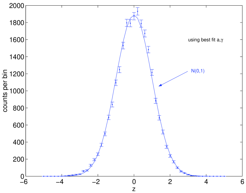
Figure 8: Histogram of rescaled diagonal deviations $z_{n}:=(\langle\phi_{n},\hat{A}\phi_{n}\rangle-\overline{A})/V_{A}(E_{n})^{1/2}$, using the best-fit power law form for Conjecture 7, compared against an appropriately-normalized Gaussian distribution of unit variance.

4.2 Quantum Unique Ergodicity (Conjecture 3)

We now examine individual diagonal matrix elements. The inset of Fig. 6 enables extreme values to be seen: it is clear that there are no anomalous extreme values which fall outside of a distribution which is condensing to the classical mean. Both the maximum 0.6811 and minimum 0.3437 of $\langle\phi_{n},\hat{A}\phi_{n}\rangle$ occur at $E_{n}<2\times 10^{4}$, visible at the far left side. This is strong evidence for QUE in this system. Since about 30000 modes are tested, the density of any excluded sequence can be given an approximate upper bound of $3\times 10^{-5}$. We note that it is possible (althouth unlikely) that by an unfortunate choice of $A$, non-uniform or scarred modes occur which do not have anomalous $\langle\phi_{n},\hat{A}\phi_{n}\rangle$ values. The only way to eliminate this possibility would be to repeat the experiment with a selection of different $A$ functions.

What is the distribution that the deviations $\langle\phi_{n},\hat{A}\phi_{n}\rangle-\overline{A}$ follow? We have rescaled these deviations according to the best-fit form of the variance in Conjecture 7, and histogram the results in Fig. 8. The distribution is consisitent with a gaussian, with an excellent quality of fit. (The slightly fatter tail on the low side is entirely due to low-lying modes; as can be seen in Fig. 6 these have a skewed distribution).

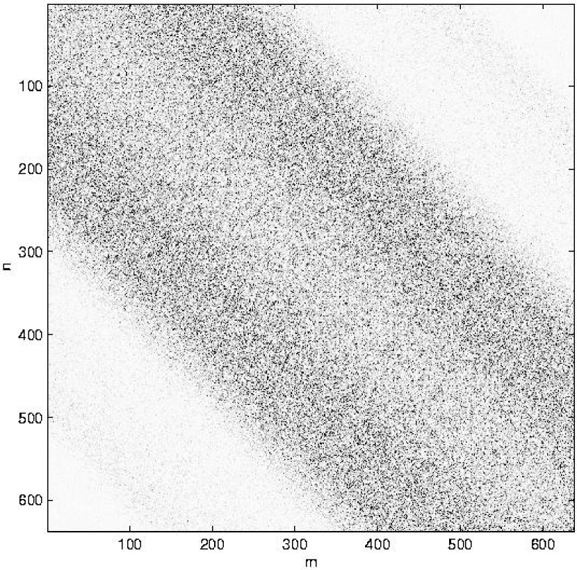
Figure 9: Density plot of block of squared matrix elements $|\langle\phi_{n},\hat{A}\phi_{m}\rangle-\delta_{nm}\overline{A}|^{2}$ for the 637 modes lying in $k\in[650,660]$. The range white to black indicates zero to $1.7\times 10^{-3}$. Individual elements appear uncorrelated, the only visible structure being the intensity varying with spectral measure (band profile).

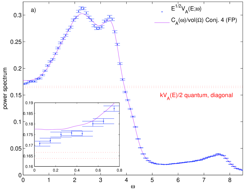
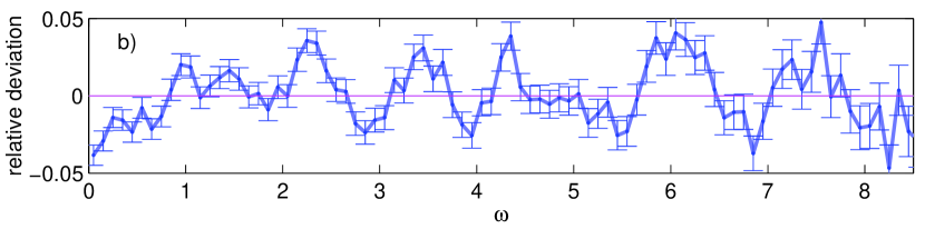
Figure 10: a) Off-diagonal quantum variance $V_{A}(E;\omega)$ (errorbars) at a single $E\approx 4.9\times 10^{5}$, as a function of distance $\omega$ (wavenumber units) from the diagonal, compared against Conjecture 4 estimated using the classical power spectrum (solid line). Errorbars are 0.7% for quantum (near the diagonal), 0.2% for classical. Also half the diagonal variance is shown as two horizontal dotted lines indicating $\pm 1$ standard deviation. Inset is a zoom on the $\omega\to 0$ region. b) Relative deviation (difference from 1 of ratio) between quantum variance and Conjecture 4.

4.3 Off-diagonal variance (Conjecture 4)

We decided, for reasons of numerical practicality, to test Conjecture 4 over a range of $\omega$, but at a single (large) value of $E$. This was performed using the single sequence of 6812 eigenfunctions with $k_{n}\in[650,750]$, from which about 2.3 million individual off-diagonal elements $\langle\phi_{n},\hat{A}\phi_{m}\rangle$ were calculated, namely those in the block $n,m:k_{n},k_{m}\in[650,660]$, the block $n,m:k_{n},k_{m}\in[660,670]$, etc, with 10 blocks in total. The first such matrix block is plotted in Fig. 9; note the strong diagonal band structure (‘band profile’ [20]). The mean off-diagonal element variances lying in successive $\omega$-intervals of width 0.1 were then collected. Thus we are testing Conjecture 4 with a window of $L(E)\approx 1.4\times 10^{5}$ and $\epsilon(E)=0.05$. Our extremely large choice of $L(E)$ allowed statistical fluctuations to be minimized (errorbars were estimated as in Section 4.1, and are generally less than 1%). We believe this is the most accurate test of the conjecture ever performed.

The resulting band profile $V_{A}(E;\omega)$ is compared against Conjecture 4 in Fig. 10. The agreement is excellent, with generally less than 3% discrepancy. Let us emphasise that there are no fitted parameters. There appears to be statistically significant deviations: the peaks and valleys (points of highest curvature, including $\omega=0$) are exaggerated more in the quantum variance than the classical. Care has been taken to ensure that this was not due to numerical errors in $\tilde{C}_{A}(\omega)$ (it was smoothed only on a much finer scale, see Appendix A). As with the diagonal variance, this may reflect slow convergence. The diagonal quantum variance, divided by $g=2$, is also shown. If step (ii) of Section 2.2 applied exactly then this would coincide with $V_{A}(E,0)$, however a $3\pm 1\%$ difference is found. It is unlikely but possible that this is merely a statistical fluctuation (a null result). Thus, at this energy, the diagonal variance prefactor discrepancy of 7% seems to result from the addition of two roughly equal effects: step (i) has about 4% discrepancy, and step (ii) about 3%. Our data does not rule out the possibility that $g$ is closer to 1.85 than to 2, which would imply slight positive correlations between neighboring eigenfunctions.

In terms of individual elements, we find no anomalously large values. This strongly supports ‘off-diagonal QUE’: the vanishing of every single off-diagonal element, a stronger result than [56]. A preliminary examination suggests uncorrelated gaussian distribution of elements, with variance given by $\omega$-distance from the diagonal, but we postpone analysis for future work.

4.4 Discussion on existence of scars

In the physics community the existence of scars is well-known, as are theoretical (non-rigorous) models. Heller [29, 30] put forward a semiclassical explanation based on enhanced short-time return probability for wavepackets launched along the least unstable periodic orbits (UPOs), which has been elaborated [15, 13, 1, 37]. Although the meaning of ‘scar’ varied historically, it is now taken to mean any deviation from the random wave prediction of eigenfunction intensity near a UPO [37]. Scar ‘strength’ depends on what test function you use to measure it [38]: in physics this test function is commonly not held fixed as the limit $E\to\infty$ is taken, rather it is chosen to collapse microlocally onto a UPO with a coordinate-space width $\sim E^{-1/4}$. By this measure, scar strength is believed not to die out in the semiclassical limit [37]. Typical scar intensities ($|\phi_{n}|^{2}$ along the UPO) do not decay, but their width, hence the associated probability mass, vanishes as $O(E^{-1/4})$.

However, in the mathematics community questions of uniformity of eigenfunctions and QUE are presented in the form of weak limits, that is, limits of matrix elements of fixed, $0^{th}$-order pseudo-differential operators. Persistence of scarring is taken to mean existence of a subsequence with $|\langle\phi_{n},\hat{A}\phi_{n}\rangle-\overline{A}|=O(1)$. Thus we might distinguish a physicist’s scar, where a probability mass vanishing as $O(E^{-1/4})$ is associated with the UPO, from a mathematician’s scar (or ‘strong scar’) which carries $O(1)$ probability mass (as in [41]).

Our results (Section 4.1) suggest strong scars do not persist asymptotically, but is consistent with the persistence of physicist’s scars, in fact giving the same power-law $|\langle\phi_{n},\hat{A}\phi_{n}\rangle-\overline{A}|=O(E^{-1/4})$ expected from scar width. Heller’s numerical demonstrations of apparently strong scarring were done at mode numbers $n\approx 2\times 10^{3}$, which, in light of our work, is well below the asymptotic regime. It is now believed by physicists that in 2D Anosov billiards strong scarring does not persist [1, 37, 33], but there still exist controversies about the width of scars [33], and in related quantum models the mechanism of scarring is an active research area [45]. Mathematically, the issue remains open.

5 Conclusions

We have studied a generic Euclidean Dirichlet billiard whose classical dynamics is Anosov, and studied quantum ergodicity of both diagonal and off-diagonal matrix elements. By accessing very high eigenvalues (100 times higher than previous studies) using the scaling method and boundary integral formulae for $\langle\phi_{n},\hat{A}\phi_{m}\rangle$ in the case of piecewise-constant test function $A$, we believe we have reached the asymptotic regime for first time. We also have unprecedented statistical accuracy due to the large number of modes computed. A summary of evidence found for the four conjectures from the Introduction is as follows:

• Conjecture 7 : Diagonal variance shows excellent agreement, with power-law $\gamma=0.479$.

• Conjecture 2 : Diagonal variance is consistent with the Feingold-Peres prediction, but with quite slow convergence (for instance, a 7% overestimate remains at $E=10^{6}$). This contrasts a random-wave model, which overestimates the fitted prefactor by 80%.

• Conjecture 3 : Compelling evidence for QUE in this system (density of exceptional subsequence $<3\times 10^{-5}$).

• Conjecture 4 : Excellent agreement for off-diagonal variance (of order $3\%$ discrepancies at $E=5\times 10^{5}$), and evidence for off-diagonal QUE.

Performing this large-scale study required limiting ourselves to one billiard $\Omega$ and one operator $A$. In order to complete the picture, the discrepancy between the predictions of Conjectures 2 and 4 and numerically-measured variances should be studied as a function of $\Omega$ and $A$.

Appendix A Classical power spectrum

We use standard techniques [27] to estimate $\tilde{C}_{A}(\omega)$. For a particular trajectory, launched with certain initial location in phase space, $A(t)$ is a noisy function (stochastic stationary process). We define its windowed Fourier transform as

$$\tilde{A}(\omega)\;:=\;\int_{0}^{T}\!A(t)e^{i\omega t}dt,$$ (27)

where the window is a ‘top-hat’ function from $0$ to $T$. Using with (10) and (9), and taking care with order of limits, we have the Wiener-Khinchin Theorem,

$$\tilde{C}_{A}(\omega)\;=\;\lim_{T\rightarrow\infty}\frac{1}{2\pi T}\,\tilde{A}^{*}(\omega)\tilde{A}(\omega).$$ (28)

For this single trajectory, $\tilde{A}(\omega)$ is a rapidly-fluctuating random function of $\omega$, with zero mean (for $\omega\neq 0$), variance given by $2\pi T\tilde{C}_{A}(\omega)$, and correlation length in $\omega$ of order $2\pi/T$. (As $T\rightarrow\infty$, the $\omega$-correlation becomes a delta-function). Thus (28) converges only in the weak sense, that is, when smoothed in $\omega$ by a finite width test function.

A given trajectory is found by solving the particle collisions with the straight and circular sections of $\Gamma$, and $A(t)$ is sampled at intervals $\Delta t=0.02$ along the trajectory (recall we assume the particle has unit speed). Then $\tilde{A}(\omega)$ is estimated using the Discrete Fourier Transform (implemented by an FFT library) of this sequence of samples, giving samples of the spectrum at $\omega$ values separated by $\Delta\omega=2\pi/T$. The correlation in $\omega$ is such that each sample is (nearly) independent. $\Delta t$ was chosen sufficiently short that aliasing (reflection of high-frequency components into apparently low frequencies) was insignificant. A trajectory length $T=10^{4}$ (about $1.8\times 10^{4}$ collisions) was used. The finiteness of $T$ causes relative errors of order $t_{\mbox{\tiny corr}}/T$, where $t_{\mbox{\tiny corr}}\approx 2$ (for our domain) is the timescale for exponential (since the billiard is Anosov) decay of correlations. Thus more sophisticated window functions are not needed.

Given $\tilde{A}(\omega)$ we use (28), with the $T$ given above, to estimate $\tilde{C}_{A}(\omega)$. We smooth in $\omega$ by a Gaussian of width $\omega_{\mbox{\tiny sm}}=0.03$. This width is chosen to be as large as possible to average the largest number of independent samples from the neighborhood of each $\omega$, but small enough to cause negligible convolution of the sharpest features of $\tilde{C}_{A}(\omega)$.

Finally, in order to reduce further the random fluctuations in the estimate, $n_{r}=6000$ independent trajectory realizations with random initial phase space locations were averaged. An estimate for the resultant relative error $\epsilon$ in $\tilde{C}_{A}(\omega)$ can be made by counting the number $N$ of independent random samples which get averaged, and using the fact that the variance of the square of a Gaussian zero-mean random variable (i.e. $\chi^{2}$ distribution with 1 degree of freedom) is twice the mean. This gives

$$\epsilon\;=\;\left(\frac{2}{N}\right)^{1/2}\;\approx\;\left(\frac{2\pi}{n_{r}\omega_{\mbox{\tiny sm}}T}\right)^{1/2},$$ (29)

which numerically has been found to be a conservative estimate. In our case $\epsilon\approx 2\times 10^{-3}$, that is, about 0.2% error.

The zero-frequency limit $\tilde{C}_{A}(0)$ is found using the smoothed $\tilde{C}_{A}(\omega)$ graph at $\omega=0$, and therefore is an average of frequencies within $O(\omega_{\mbox{\tiny sm}})$ of zero. This is justified because correlation decay (weak mixing) causes all moments of $C_{A}(\tau)$ to be finite, hence there is no singularity in $\tilde{C}_{A}(\omega)$ at $\omega=0$ (it can be expanded in an even Taylor series about $\omega=0$ with finite coefficients).

Appendix B Scaling method for the Dirichlet eigenproblem

The scaling method for the solution of the Dirichlet eigenproblem in star-shaped domains was invented by Vergini and Saraceno [53], and considering its great efficiency it has received remarkably little attention. Here we give only an outline.

The method relies on the remarkable fact that the normal derivatives of eigenfunctions lying close in energy are ‘quasi-orthogonal’ (nearly orthogonal) on the boundary, with respect to the boundary weight function $r_{n}:={\mathbf{r}}\cdot{\mathbf{n}}$.

Lemma B.1

Let $\Omega\in\mathbb{R}^{d}$, $d\geq 2$ be a Lipshitz domain with boundary $\Gamma$ and Dirichlet spectral data $\{E_{j}\}$, $\{\phi_{j}\}$. Let ${\mathbf{n}}$ and ${\mathbf{r}}$ be defined as in Lemma 3.1, with $r_{n}:={\mathbf{r}}\cdot{\mathbf{n}}$. Then, for all $i\geq 1$, $j\geq 1$,

$$Q_{ij}:=\oint_{\Gamma}\!r_{n}({\mathbf{n}}\cdot\nabla\phi_{i})({\mathbf{n}}\cdot\nabla\phi_{j})\,ds\;=\;2E_{i}\delta_{ij}+\frac{(E_{i}-E_{j})^{2}}{4}\langle\phi_{i},r^{2}\phi_{j}\rangle_{\Omega},$$ (30)

This is proved in App. C. A corollary is that, since $r^{2}:={\mathbf{r}}\cdot{\mathbf{r}}$ is a bounded operator on the domain, off-diagonal elements of $Q$ must vanish quadratically as one approaches the diagonal. Thus the matrix with elements $Q_{ij}/2E_{i}$ approximates the identity matrix, when restricted to an energy window $E_{i},E_{j}\in[E-\epsilon_{0},E+\epsilon_{0}]$, if the window size remains relatively narrow $\epsilon_{0}=o(E^{1/2})$.

We choose a ‘center’ wavenumber $k=E^{1/2}$, near which we are interested in extracting eigenfunctions, and relative to which the wavenumber shift of mode $i$ is $\omega_{i}(k):=k-k_{i}$. Consider an eigenfunction $\phi_{i}$ for which $\omega_{i}<0$ and $|\omega_{i}|\ll O(1)$. We create a version spatially rescaled (dilated about the origin) by an amount needed to bring its wavenumber to $k$, that is, $\chi_{i}(k,{\mathbf{r}}):=\phi_{i}(k{\mathbf{r}}/k_{i})$. We call this function $k$-rescaled. Thus we have $-\Delta\chi_{i}=E\chi_{i}$ everywhere inside $\Omega$, with $\chi_{i}(k,{\mathbf{r}})=0$ on the rescaled boundary (i.e. for all $k{\mathbf{r}}/k_{i}\in\Gamma$). The rescaled eigenfunction can be Taylor expanded in $\omega_{i}$,

$$\chi_{i}(k,{\mathbf{r}}) = \phi_{i}\left({\mathbf{r}}+\frac{\omega_{i}}{k_{i}}{\mathbf{r}}\right)\;=\;\phi_{i}({\mathbf{r}})+\frac{\omega_{i}}{k_{i}}{\mathbf{r}}\cdot\nabla\phi_{i}+O(\omega^{2})$$ (31)

$$= \frac{\omega_{i}}{k_{i}}r_{n}{\mathbf{n}}\cdot\nabla\phi_{i}+O(\omega^{2})\qquad\mbox{for }{\mathbf{r}}\in\Gamma,$$

where Dirichlet boundary conditions were applied. We construct a basis of $N$ functions $\xi_{l}(k,{\mathbf{r}})$, satisfying $-\Delta\xi_{l}=E\xi_{l}$ inside $\Omega$, no particular boundary conditions on $\Gamma$, and non-orthogonal over $\Omega$. We assume they approximately span the linear space in which rescaled eigenfunctions live, so that

$$\chi_{i}(k,{\mathbf{r}})\;=\;\sum_{l=1}^{N}X_{li}\,\xi_{l}(k,{\mathbf{r}})\;+\;\epsilon_{i}({\mathbf{r}})\qquad\mbox{for all $i$ of interest},$$ (32)

where the error $\epsilon_{i}$ can be made negligibly small for some $N$. In practise $N$ need exceed ${N_{\mbox{\tiny sc}}}$ defined in (24) by only a small factor (2 or less). Our goal is then to solve for a shift $\omega_{i}$ and the corresponding $i^{th}$ column of the coefficient matrix $X$. We can do this by simultaneous diagonalization of quadratic forms. We define two symmetric bilinear forms on the boundary,

$$f(u,v) := \oint_{\Gamma}\frac{1}{r_{n}}uv\,{d{\mathbf{s}}},$$ (33)

$$g(u,v) := \frac{1}{k}\oint_{\Gamma}\frac{1}{r_{n}}(u{\mathbf{r}}\cdot\nabla v+v{\mathbf{r}}\cdot\nabla u)\,{d{\mathbf{s}}}.$$ (34)

Note that defining these forms brings the extra requirement that the domain be strictly star-shaped about the origin ($r_{n}>0$), which from now on we assume. In the rescaled eigenbasis $f$ is, via (31) and (30)

$$f(\chi_{i},\chi_{j})\;=\;\frac{\omega_{i}\omega_{j}}{k_{i}k_{j}}Q_{ij}+O(\omega^{3})\;=\;2\omega_{i}^{2}\delta_{ij}+O(\omega^{3}),$$ (35)

a matrix which is close to diagonal, because of the closeness of $Q$ to the identity. In the same basis, recognizing that for $k$-rescaled functions $g$ is equivalent to $df/dk$, the derivative of (34) with respect to the center wavenumber, and using $d\omega_{i}/dk=1$, we have

$$g(\chi_{i},\chi_{j})\;=\;\frac{\omega_{i}+\omega_{j}}{k_{i}k_{j}}Q_{ij}+O(\omega^{2})\;=\;4\omega_{i}\delta_{ij}+O(\omega^{2}),$$ (36)

so $g$ is also close to diagonal. Thus the set $\{\chi_{i}\}$ with small $|\omega_{i}|$ approximately diagonalizes both bilinear forms, with the approximation error growing as a power of $|\omega_{i}|$. As we explain below, in practise the converse applies, that is, by simultaneously diagonalizing $f$ and $g$ we can extract the set of eigenfunctions $\{\chi_{i}\}$ with smallest $|\omega_{i}|$. Therefore, loosely speaking, when the boundary weight function $1/r_{n}$ is used, domain eigenfunctions are given by the simultaneous eigenfunctions of the (squared) boundary norm and its $k$-derivative.

We perform the diagonalization in the basis (32). That is, matrices $F_{lm}:=f(\xi_{l},\xi_{m})$ and $G_{lm}:=g(\xi_{l},\xi_{m})$, with $l,m=1\cdots N$, are filled. This requires basis and first derivative evaluations on the boundary. It is an elementary fact that given a positive matrix $F$ and a symmetric matrix $G$ there exists a square matrix $Y$ and a diagonal matrix $D:=\mbox{diag}\{\mu_{i}\}$ which satisfy $Y^{T}FY=I$ and $Y^{T}GY=D$. The matrices $Y$ and $D$ can be found by standard numerical diagonalization algorithms in $O(N^{3})$ time. If (35) and (36) held without error terms, and the number of modes $i$ for which they held were equal to (or exceeded) the basis size $N$, then we would be able directly to equate the columns of $Y$ with the desired columns of $X$ (barring permutations). In this case $\omega_{i}=2/\mu_{i}$ would also hold, from which the desired wavenumbers $k_{i}$ follow. However, using Weyl’s law and (24) is follows that such a large number of modes requires that the largest $|\omega_{i}|$ is of order unity, in which case errors in (35) and (36) would become unacceptable. It is an empirical observation found through numerical study that in fact columns of $Y$ corresponding to the largest magnitude generalized eigenvalues $\mu_{i}$ (and therefore the smallest shifts $|\omega_{i}|$) do accurately match columns of $X$. Thus perturbations by other vectors in the span of basis functions are small. Further discussion is postponed to a future publication [11].

We mention a couple of other implementation details. Because the generalized eigenproblem turns out to be singular it is truncated to its non-singular part [53, 7]. If columns of $Y$ are normalized such that $Y^{T}FY=I$ holds then the resulting eigenfunctions can be normalized over $\Omega$ by dividing the $i^{th}$ column of $Y$ by $\sqrt{2}\omega_{i}$. Depending on the choice of basis, spurious solutions can result; they are easily identified because their norm over $\Omega$, computed by the following Rellich identity, is not close to 1.

Lemma B.2 (Rellich)

With the definitions of Lemma B.1, for all $j\geq 1$,

$$\frac{1}{2E_{j}}\oint_{\Gamma}\!r_{n}({\mathbf{n}}\cdot\nabla\phi_{j})^{2}\,ds\;=\;1$$ (37)

This identity is a special case of Lemma 3.1 found by substituting $\Omega_{A}=\Omega$, $u=v=\phi_{j}$, and $E=E_{j}$, and recognising ${\mathbf{r}}\cdot\nabla\phi_{j}=r_{n}{\mathbf{n}}\cdot\nabla\phi_{j}$. The maximum $|\omega_{i}|$ in which levels of useful accuracy are found is of order $0.2/R$ where $R$ is the largest radius of the domain. The lack of missing modes obtained with this method is illustrated by Fig. 5. There are several implementation issues and improvements that we do not have space to discuss here [53, 7, 11].

A word about the basis set choice $\{\xi(k,{\mathbf{r}})\}$, $1\leq i\leq N$, is needed. Until now plane waves (including evanescent plane waves [53]) or regular Bessel functions [19] have been used. These fail for non-convex domain shapes, or those with corners, thus to tackle the domain in this study a basis of irregular Bessel (i.e. Neumann) functions, placed at equal intervals along a curve $\Gamma^{+}$ exterior to $\Omega$, was developed by the author. $\Gamma^{+}$ is defined as the set of points whose nearest distance to $\Gamma$ is $D$, with $kD=7$ (roughly one wavelength distant). This was found to handle (non-reentrant) corners successfully. It performs extremely well for all shapes that have been attempted so far. The basis size $N$ is about $1.5{N_{\mbox{\tiny sc}}}$ (see (24)), thus, depending on required accuracy, about $N/20$ useful modes are found per dense matrix diagonalization ($O(N^{3})$ effort). This is $O(N)$ faster than other boundary methods; we remind the reader that $N$ is larger than $10^{3}$ in our work.

Appendix C Identities involving eigenfunctions of the Laplacian

Let there be constants $E_{u}>0$, $E_{v}>0$, and let $-\Delta u=E_{u}u$ and $-\Delta v=E_{v}v$ hold in a Lipschitz domain $\Omega_{A}\in\mathbb{R}^{d}$, for some general dimension $d\geq 2$. The following expressions for the divergence of certain vector fields result from elementary calculus. By $\nabla\nabla u$ we mean the second derivative tensor (dyad).

$$\nabla\cdot(v\nabla u) = -E_{u}uv+\nabla u\cdot\nabla v$$ (38)

$$\nabla\cdot({\mathbf{r}}uv) = duv+u{\mathbf{r}}\cdot\nabla v+v{\mathbf{r}}\cdot\nabla u$$ (39)

$$\nabla\cdot({\mathbf{r}}\nabla u\cdot\nabla v) = d\nabla u\cdot\nabla v+\nabla u\cdot\nabla\nabla v\cdot{\mathbf{r}}+\nabla v\cdot\nabla\nabla u\cdot{\mathbf{r}}$$ (40)

$$\nabla\cdot[({\mathbf{r}}\cdot\nabla u)\nabla v] = \nabla u\cdot\nabla v-E_{v}v{\mathbf{r}}\cdot\nabla u+\nabla v\cdot\nabla\nabla u\cdot{\mathbf{r}}$$ (41)

$$\nabla\cdot(r^{2}v\nabla u) = 2v{\mathbf{r}}\cdot\nabla u-E_{u}r^{2}uv+r^{2}\nabla u\cdot\nabla v$$ (42)

First we prove Lemma 3.1 (also see App. H of [7]). Consider the following four equations: (39), (40), (41), and its counterpart obtained by swapping $u$ and $v$. Integrating each of these over $\Omega_{A}$, then applying the Divergence Theorem, gives four expressions for surface integrals in terms of domain integrals. Substituting these into the right-hand side of the expression in Lemma 3.1, and setting $E_{u}=E_{v}=E$, gives, after cancellation, the left-hand side.

A similar but more complicated technique proves Lemma B.1. First we consider modes $i,j$ which are non-degenerate, that is, $E_{i}\neq E_{j}$. Eight equations are needed: the four mentioned above, then (38) and (42) and their counterparts swapping $u$ and $v$. Each should be integrated over $\Omega$ and the Divergence Theorem applied. The following identity may then be verified by substitution of the eight resulting equations into its right-hand side. Using the abbreviations $\varepsilon:=E_{u}-E_{v}$, ${\cal E}:=E_{u}+E_{v}$, $u_{n}={\mathbf{n}}\cdot\nabla u$, $u_{r}={\mathbf{r}}\cdot\nabla u$, the identity to be checked is,

$$\frac{\varepsilon^{2}}{4}\int_{\Omega}r^{2}uv\,d{\mathbf{r}}\;=\;\oint_{\Gamma}\!\frac{d-2}{2}(u_{n}v+v_{n}u)+\left(\frac{\cal E}{\varepsilon}-\frac{\varepsilon}{4}r^{2}\right)(u_{n}v-v_{n}u)\\ +r_{n}\left(\frac{\cal E}{2}uv-\nabla u\cdot\nabla v\right)+u_{r}v_{n}+v_{r}u_{n}\,ds.$$ (43)

The substitutions $u=\phi_{i}$, $v=\phi_{j}$, $E_{u}=E_{i}$ and $E_{v}=E_{j}$, and applying Dirichlet boundary conditions, turns the right-hand side into $Q_{ij}$. More details about how such identities are found using a symbolic matrix method will be postponed to a future publication [10].

Finally, the other possibility is that $E_{i}=E_{j}$ (which need not imply $i=j$). We take Lemma 3.1 with the choices $\Omega_{A}=\Omega$, $u=\phi_{i}$, $v=\phi_{j}$, $E_{i}=E_{j}=E$, apply Dirichlet boundary conditions, and use orthonormality (3). Thus Lemma B.1 is proved for all choices of $i,j$.

References

- [1] O. Agam and S. Fishman, “Semiclassical criterion for scars of wavefunctions in chaotic systems”, Phys. Rev. Lett. 73 806–809 (1994).
- [2] R. Aurich and M. Taglieber, “On the rate of quantum ergodicity on hyperbolic surfaces and for billiards”, Physica D 118, 84–102 (1998).
- [3] E. J. Austin and M. Wilkinson, “Distribution of matrix elements of a classicaly chaotic system”, Europhys. Lett. 20, 589–593 (1992).
- [4] A. Bäcker, R. Schubert, and P. Stifter, “On the number of bouncing ball modes in billiards”, J. Phys. A, 30, 6783–95 (1997).
- [5] A. Bäcker, R. Schubert, and P. Stifter, “Rate of quantum ergodicity in Euclidean billiards”, Phys. Rev. E 57, 5425–47 (1998); also see Errata for this paper, Phys. Rev. E 58 (4) (1998).
- [6] A. Bäcker, “Numerical aspects of eigenvalue and eigenfunction computations for chaotic quantum systems”, in The Mathematical Aspects of Quantum Maps, M. Degli Esposti and S. Graffi (Eds.) Springer Lecture Notes in Physics 618, 91-144 (2003).
- [7] A. H. Barnett, Ph. D. thesis, Harvard University, 2000.
- [8] A. H. Barnett, D. Cohen, and E. J. Heller, Phys. Rev. Lett. 85, 1412 (2000).
- [9] A. H. Barnett, D. Cohen, and E. J. Heller, Rate of energy absorption for a driven chaotic cavity”, J. Phys. A 34, 413–437 (2001).
- [10] A. H. Barnett, “Quasi-orthogonality on the boundary for Euclidean Laplace eigenfunctions”, preprint, math-ph/0601006
- [11] A. H. Barnett, “The scaling method for the Dirichlet eigenproblem”, in preparation.
- [12] M. V. Berry, “Regular and irregular semiclassical wavefunctions”, J. Phys. A 10 2083–91 (1977).
- [13] M. V. Berry, in “Les Houches Lecture Notes, Summer School on Chaos and Quantum Physics” (M.-J. Giannoni, A. Voros, and J. Zinn-Justin, Eds.), Elsevier Science, Amsterdam, 1991; M. V. Berry, Proc. Roy. Soc. A 243 219 (1989).
- [14] T. Betcke and L. N. Trefethen, “Reviving the Method of Particular Solutions”, SIAM Review 47, 469–491 (2005).
- [15] E. B. Bogomolny, “Smoothed wave functions of chaotic quantum systems”, Physica D 31, 169–189 (1988).
- [16] E. B. Bogomolny, B. Georgeot, M. Giannoni, and C. Schmidt, “Chaotic billiards generated by arithmetic groups”, Phys. Rev. Lett. 69, 1477–80 (1992).
- [17] O. Bohigas, “Random matrix theories and chaotic dynamics”, in Chaos et physique quantique (Les Houches, 1989), 87–199, M. J. Giannoni, A. Voros, and J. Zinn-Justin, eds, (North-Holland, Amsterdam, 1991).
- [18] D. Boosé and J. Main, “Distributions of transition matrix elements in classically mixed quantum systems”, Phys. Rev. E 60, 2813–44 (1999).
- [19] G. Casati and T. Prosen, “The quantum mechanics of chaotic billiards”, Physica D 131, 293–310 (1999).
- [20] D. Cohen, “Chaos and energy spreading for time-Dependent Hamiltonians, and the various Regimes in the theory of Quantum Dissipation”, Ann. Phys. (N.Y.) 283, 175–231 (2000).
- [21] Y. Colin de Verdière, “Ergodicité et fonctions propres du laplacien”, Comm. Math. Phys. 102 497 (1985).
- [22] M. Combescure and D. Robert, “Semiclassical sum rules and generalized coherent states”, J. Math. Phys. 36, 6596–6610 (1995).
- [23] H. Donnelly, “Quantum Unique Ergodicity”, Proc. Am. Math. Soc. 131, 2945–51 (2003).
- [24] B. Eckhardt, S. Fishman, J. Keating, O. Agam, J. Main, and K. Müller, “Approach to ergodicity in quantum wave functions”, Phys. Rev. E 52, 5893–5903 (1995).
- [25] F. Faure, S. Nonnenmacher, and S. De Bièvre, “Scarred eigenstates for quantum cat maps of minimal periods”, Comm. Math. Phys. 239 449–492 (2003).
- [26] M. Feingold and A. Peres, “Distribution of matrix elements of chaotic systems”, Phys. Rev. A, 34, 591 (1986).
- [27] C. V. Gardiner, Handbook of Stochastic Methods for physics, chemistry, and the natural sciences, 2nd Ed. (Springer-Verlag, 1997).
- [28] M. C. Gutzwiller, Chaos in Classical and Quantum Mechanics, (Springer, NY, 1990).
- [29] E. J. Heller, “Bound-state eigenfunctions of classically chaotic hamiltonian systems: scars of periodic orbits”, Phys. Rev. Lett. 1515–18 (1984).
- [30] E. J. Heller, “Wavepacket dynamics and quantum chaology”, in Chaos et physique quantique (Les Houches, 1989), 547–664, M. J. Giannoni, A. Voros, and J. Zinn-Justin, eds, (North-Holland, Amsterdam, 1991).
- [31] S. Hortikar and M. Srednicki, “Random matrix elements and eigenfunctions in chaotic systems”, Phys. Rev. E 57, 7313–16 (1998).
- [32] J. R. Kuttler and V. G. Sigillito, “Eigenvalues of the Laplacian in two dimensions”, SIAM Review, 26, 163–193 (1984).
- [33] B. Li and B. Hu, J. Phys. A 31, 483 (1998).
- [34] E. Lindenstrauss, “Invariant measures and arithmetic quantum unique ergodicity”, Annals of Math. (to appear).
- [35] W. Luo and P. Sarnak, “Quantum variance for Hecke eigenforms”, Annales Scient. de l’École Norm. Sup. 37, 769–799 (2004).
- [36] A. Martinez, An Introduction to Semiclassical and Microlocal Analysis, (Springer, 2002).
- [37] L. Kaplan and E. J. Heller, “Linear and nonlinear theory of eigenfunction scars”, Ann. Phys. 264, 171–206 (1998).
- [38] L. Kaplan and E. J. Heller, “Measuring scars of periodic orbits”, Phys. Rev. E 59, 6609–28 (1999).
- [39] T. Prosen, “Statistical properties of matrix elements in a Hamilton system between integrability and chaos”, Ann. Phys. N.Y. 235, 115–164 (1994).
- [40] T. Prosen, “Quantization of a generic chaotic 3D billiard with smooth boundary. I. Energy level statistics”, Phys. Lett. A 233, 323–331 (1997); T. Prosen, “Quantization of a generic chaotic 3D billiard with smooth boundary. II. Structure of high-lying eigenstates”, Phys. Lett. A 233, 332–342 (1997).
- [41] Z. Rudnick and P. Sarnak, “The behaviour of eigenstates of arithmetic hyperbolic manifolds”, Comm. Math. Phys. 161 195–213 (1994).
- [42] P. Sarnak, “Arithmetic quantum chaos”, The Schur lectures (Tel Aviv, 1992), Israel Math. Conf. Proc. 8, 183–236 (Bar-Ilan University, 1995).
- [43] P. Sarnak, “Spectra and eigenfunctions of Laplacians”, in Partial Differential Equations and Their Applications (CRM Proceedings and Lecture Notes, Vol 12) pp. 261–276 (American Mathematical Society, 1997).
- [44] P. Sarnak, “Spectra of Hyperbolic Surfaces”, Bulletin of the AMS, 40, 441–478 (2003).
- [45] H. Schanz and T. Kottos, “Scars on quantum networks ignore the Lyapunov exponent”, Phys. Rev. Lett. 90, 234101 (2003).
- [46] A. I. Schnirelman, Usp. Mat. Nauk. 29, 181 (1974).
- [47] Ya. G. Sinai, “Dynamical systems with elastic reflections: ergodic properties of dispersing billiards”, Russ. Math. Surveys 25, 137–189 (1970).
- [48] D. S. Sivia, Data Analysis: A Bayesian Tutorial, (Oxford, 1996).
- [49] F. Steiner, “Quantum Chaos”, chao-dyn/9402001 (1994).
- [50] G. Tanner, “How chaotic is the stadium billiard? A semiclassical analysis”, J. Phys. A 30, 2863–88 (1997).
- [51] T. Tate, “Some remarks on the off-diagonal asymptotics in quantum ergodicity”, Asym. Anal. 19, 289–296 (1999).
- [52] G. Veble, M. Robnik, and J. Liu, “Study of regular and irregular states in generic systems”, J. Phys. A 32, 6423–44 (1999).
- [53] E. Vergini and M. Saraceno, Phys. Rev. E, 52, 2204 (1995); E. Vergini, Ph. D. thesis, Universidad de Buenos Aires, 1995.
- [54] M. Wilkinson, “A semiclassical sum rule for matrix elements of classically chaotic systems”, J. Phys. A 20, 2415–23 (1987).
- [55] S. Zelditch, “Uniform distribution of eigenfunctions on compact hyperbolic surfaces”, Duke Math. J. 55, 919 (1987).
- [56] S. Zelditch, “Quantum transition amplitudes for ergodic and for completely integrable systems”, J. Funct. Anal. 94, 415–436 (1990).
- [57] S. Zelditch, “Quantum ergodicity on the sphere”, Comm. Math. Phys. 146, 61–71 (1992).
- [58] S. Zelditch, “On the rate of quantum ergodicity I: Upper Bounds”, Comm. Math. Phys. 160, 81–92 (1994).
- [59] S. Zelditch, “On the rate of quantum ergodicity II: Lower Bounds”, Comm. Partial Diff. Eqns. 19, 1565–79 (1994).
- [60] S. Zelditch, “Quantum mixing”, J. Func. Anal. 140, 68–86 (1996).
- [61] S. Zelditch, “A random matrix model for quantum mixing”, Int. Math. Res. Not. 3 115–137 (1996).
- [62] S. Zelditch and M. Zworski, “Ergodicity of eigenfunctions for ergodic billiards”, Comm. Math. Phys., 175 673–682 (1996).
- [63] S. Zelditch, “Quantum ergodicity and mixing of eigenfunctions”, Elsevier Encyclopedia of Mathematical Physics, preprint (2005), math-ph/0503026