MIMO Channel Correlation in General Scattering Environments

Abstract

This paper presents an analytical model for the fading channel correlation in general scattering environments. In contrast to the existing correlation models, our new approach treats the scattering environment as non-separable and it is modeled using a bi-angular power distribution. The bi-angular power distribution is parameterized by the mean departure and arrival angles, angular spreads of the univariate angular power distributions at the transmitter and receiver apertures, and a third parameter, the covariance between transmit and receive angles which captures the statistical interdependency between angular power distributions at the transmitter and receiver apertures. When this third parameter is zero, this new model reduces to the well known “Kronecker” model. Using the proposed model, we show that Kronecker model is a good approximation to the actual channel when the scattering channel consists of a single scattering cluster. In the presence of multiple remote scattering clusters we show that Kronecker model over estimates the performance by artificially increasing the number of multipaths in the channel.

I Introduction

Wireless channel modelling has received much attention in recent years since space-time processing using multiple antennas is becoming one of the most promising areas for improvements in performance of mobile communication systems [1, 2]. In channel modelling research, the effects of fading channel correlation due to insufficient antenna spacing and sparse scattering environments are of primary concern as they impact the performance of multiple-input multiple-output (MIMO) communication systems.

A popular channel model that has been used in MIMO performance analysis is the “Kronecker” model [3, 4, 5]. In this model, the correlation properties of the MIMO channel are modeled at the transmitter and receiver separately, neglecting the statistical interdependency between scattering distributions at the transmitter and receiver antenna apertures. Measurement and analytical results presented in [6, 7] suggest that the Kronecker model does not accurately model the underlying scattering channel, therefore it does not provide accurate performance results.

In this paper, using a recently proposed spatial channel model [8], we develop an alternate to the Kronecker model which gives channel correlation for a general class of scattering environments. In our proposed model, fading channel correlation is parameterized by the antenna configuration details (spacing and the placement) both at the transmitter and the receiver arrays, and the joint bi-angular power distribution between transmitters and receivers, which models the scattering environment surrounding the transmit and receive antenna apertures. The bi-angular power distribution is parameterized by the mean departure and arrival angles, angular spreads of the univariate angular power distributions at the transmitter and receiver apertures, and a third parameter, the covariance between transmit and receive angles which captures the statistical interdependency between angular power distributions at the transmitter and receiver apertures. When this third parameter is zero, i.e., the power distribution at the transmitter is independent of the power distribution at the receiver, the proposed correlation model reduces to the Kronecker model. In order to model the scattering environment we propose several bi-angular power distributions and also find the correlation coefficients associated with these distributions in closed form. Using the proposed model, we show that Kronecker model is a good approximation to the actual channel when the scattering channel consists of a single scattering cluster. We also show that when the scattering channel consists of multiple remote scattering clusters, the Kronecker model over estimates the performance MIMO systems by artificially increasing the number of scattering clusters in the scattering channel.

Notations: Throughout the paper, the following notations will be used: Bold lower (upper) letters denote vectors (matrices). ${[\cdot]}^{T}$, ${[\cdot]}^{\ast}$ and ${[\cdot]}^{\dagger}$ denote the transpose, complex conjugate and conjugate transpose operations, respectively. The symbols $\delta(\cdot)$ and $\otimes$ denote the Dirac delta function and Matrix Kronecker product, respectively. The notation $E\left\{\cdot\right\}$ denotes the mathematical expectation,$\operatorname{vec}({\boldsymbol{A}})$ denotes the vectorization operator which stacks the columns of $\boldsymbol{A}$, $\lceil{.}\rceil$ denotes the ceiling operator and $\mathbb{S}^{1}$ denotes the unit circle.

II Spatial Channel Model

First we review the spatial channel model proposed in [8]. Consider a MIMO system consisting of $n_{T}$ transmit antennas located at positions $\boldsymbol{x}_{t}$, $t=1,2,\cdots,n_{T}$ relative to the transmitter array origin, and $n_{R}$ receive antennas located at positions $\boldsymbol{y}_{r}$, $r=1,2,\cdots,n_{R}$ relative to the receiver array origin. $r_{T}\geq\max\parallel\!\!\boldsymbol{x}_{t}\!\!\parallel$ and $r_{R}\geq\max\parallel\!\!\boldsymbol{y}_{r}\!\!\parallel$ denote the radius of spheres that contain all the transmitter and receiver antennas, respectively. We assume that scatterers are distributed in the far field from the transmitter and receiver antennas and regions containing the transmit and receive antennas are distinct.

By taking into account physical aspects of scattering, the MIMO channel matrix $\boldsymbol{H}$ can be decomposed into deterministic and random parts as [8]

$$\boldsymbol{H} =\boldsymbol{J}_{R}\boldsymbol{H}_{S}{\boldsymbol{J}}^{\dagger}_{T},$$ (1)

where $\boldsymbol{J}_{R}$ is the receiver configuration matrix,

$$\boldsymbol{J}_{R} =\left[\begin{array}[]{ccc}{\mathcal{J}}_{-M_{R}}(\boldsymbol{v}_{1})&\cdots&{\mathcal{J}}_{M_{R}}(\boldsymbol{v}_{1})\\ {\mathcal{J}}_{-M_{R}}(\boldsymbol{v}_{2})&\cdots&{\mathcal{J}}_{M_{R}}(\boldsymbol{v}_{2})\\ \vdots&\ddots&\vdots\\ {\mathcal{J}}_{-M_{R}}(\boldsymbol{v}_{n_{R}})&\cdots&{\mathcal{J}}_{M_{R}}(\boldsymbol{v}_{n_{R}})\\ \end{array}\right],$$ (6)

and $\boldsymbol{J}_{T}$ is the transmitter configuration matrix,

$$\boldsymbol{J}_{T} =\left[\begin{array}[]{ccc}{\mathcal{J}}_{-M_{T}}(\boldsymbol{u}_{1})&\cdots&{\mathcal{J}}_{M_{T}}(\boldsymbol{u}_{1})\\ {\mathcal{J}}_{-M_{T}}(\boldsymbol{u}_{2})&\cdots&{\mathcal{J}}_{M_{T}}(\boldsymbol{u}_{2})\\ \vdots&\ddots&\vdots\\ {\mathcal{J}}_{-M_{T}}(\boldsymbol{u}_{n_{T}})&\cdots&{\mathcal{J}}_{M_{T}}(\boldsymbol{u}_{n_{T}})\\ \end{array}\right],$$ (11)

where ${\mathcal{J}}_{n}(\boldsymbol{x})$ is the spatial-to-mode function (SMF) which maps the antenna location to the $n$-th mode of the region. The form which the SMF takes is related to the shape of the scatterer-free antenna region. For a circular region in 2-dimensional space, the SMF is given by a Bessel function of the first kind [8] and for a spherical region in 3-dimensional space, the SMF is given by a spherical Bessel function [9]. For a prism-shaped region, the SMF is given by a prolate spheroidal function [10].

Here we consider the situation where the multipath is restricted to the azimuth plane only (2-D scattering environment), having no field components arriving at significant elevations. In this case, the SMF is given by

$${\mathcal{J}}_{n}(\boldsymbol{w})\, {\triangleq}\,J_{n}(k\|\boldsymbol{w}\|)e^{{\imath}n(\phi_{w}-\pi/2)},$$

where $J_{n}(\cdot)$ is the Bessel function of integer order $n$, vector $\boldsymbol{w}\>\equiv\>(\|\boldsymbol{w}\|,\phi_{w})$ in polar coordinates is the antenna location relative to the origin of the aperture which encloses the antennas, $k=2\pi/\lambda$ is the wave number with $\lambda$ being the wave length and $\imath=\sqrt{-1}$. $\boldsymbol{J}_{T}$ is $n_{T}{\times}(2M_{T}+1)$ and $\boldsymbol{J}_{R}$ is $n_{R}{\times}(2M_{R}+1)$, where $2M_{T}+1$ and $2M_{R}+1$ are the number of effective communication modes at the transmit and receive regions, respectively. Note, $M_{T}$ and $M_{R}$ are defined by the size of the regions containing all the transmit and receive antennas, respectively [11]. In our case,

$$M_{T} =\left\lceil{\frac{ker_{T}}{\lambda}}\right\rceil\text{\quad and }M_{R}=\left\lceil{\frac{ker_{R}}{\lambda}}\right\rceil,$$

where $e\approx{2.7183}$.

Finally, $\boldsymbol{H}_{S}$ is the $(2M_{R}+1)\times(2M_{T}+1)$ random complex scattering channel matrix with $(\ell,m)$-th element given by

$$\left\{\boldsymbol{H}_{S}\right\}_{\ell,m} =\iint_{\mathbb{S}^{1}\times\mathbb{S}^{1}}\!g(\phi,\varphi)e^{\imath(m-M_{T}-1)\phi}e^{-\imath(\ell-M_{R}-1)\psi}\mathrm{d\phi}\mathrm{d\varphi}$$ (12)

representing the complex scattering gain between the $(m-M_{T}-1)$-th mode of the scatter-free transmit region and $(\ell-M_{R}-1)$-th mode of the scatter-free receiver region, where $g(\phi,\varphi)$ is the effective random complex scattering gain function for signals with angle-of-departure $\phi$ from the scatter-free transmitter region and angle-of-arrival $\varphi$ at the scatter-free receiver region. The reader is referred to [8] for more information about the channel decomposition (1).

The correlation matrix of the MIMO channel $\boldsymbol{H}$ given by (1) can be written as

$$\boldsymbol{R}=E\left\{\boldsymbol{h}{\boldsymbol{h}}^{\dagger}\right\}=\left({\boldsymbol{J}}^{\ast}_{T}\otimes\boldsymbol{J}_{R}\right)\boldsymbol{R}_{S}({\boldsymbol{J}}^{T}_{T}\otimes{\boldsymbol{J}}^{\dagger}_{R}),$$

where $\boldsymbol{h}=\operatorname{vec}{(\boldsymbol{H})}$ and $\boldsymbol{R}_{S}$ the modal correlation matrix of the scattering channel,

$$\boldsymbol{R}_{S}=E\left\{\boldsymbol{h}_{S}{\boldsymbol{h}}^{\dagger}_{S}\right\},$$

with $\boldsymbol{h}_{S}=\operatorname{vec}{(\boldsymbol{H}_{S})}$. Modal correlation matrix $\boldsymbol{R}_{S}$ can also be written as a block matrix of $(2M_{T}+1)\times(2M_{T}+1)$ blocks, each of size $(2M_{R}+1)\times(2M_{R}+1)$,

$$\boldsymbol{R}_{S} \!=\!\left[\begin{array}[]{cccc}\!\!\boldsymbol{R}_{S,1,1}\!&\boldsymbol{R}_{S,1,2}\!&\!\cdots\!&\boldsymbol{R}_{S,1,2M_{T}+1}\!\!\\ \!\!\boldsymbol{R}_{S,2,1}\!&\boldsymbol{R}_{S,2,2}\!&\!\cdots\!&\boldsymbol{R}_{S,2,2M_{T}+1}\!\!\\ \!\!\vdots\!&\vdots\!&\!\ddots\!&\vdots\!\!\\ \!\!\boldsymbol{R}_{S,2M_{R}+1,1}\!&\boldsymbol{R}_{S,2M_{R}+1,2}\!&\!\cdots\!&\boldsymbol{R}_{S,2M_{R}+1,2M_{T}+1}\!\!\\ \end{array}\right],$$ (17)

where $\boldsymbol{R}_{S,m,m^{\prime}}$ is the correlation between $m$-th and $m^{\prime}$-th columns of $\boldsymbol{H}_{S}$. A diagonal block $\boldsymbol{R}_{S,m,m}$ gives the modal correlation matrix at the receiver region due to the $m$-th mode at the transmit region whereas off diagonal blocks $\boldsymbol{R}_{S,m,m^{\prime}}$ give the cross correlation between two distinct modal pairs at the transmit and receiver apertures.

II-A Modal Correlation in General Scattering Environments

Using (12), we can define the modal correlation between complex scattering gains as

$$\gamma_{m,m^{\prime}}^{\ell,\ell^{\prime}} \triangleq E\left\{\{\boldsymbol{H}_{S}\}_{\ell,m}{\{\boldsymbol{H}_{S}\}}^{\ast}_{\ell^{\prime},m^{\prime}}\right\}.$$ (18)

Substituting (12) in (18) gives

$$\gamma_{m,m^{\prime}}^{\ell,\ell^{\prime}}\!\! =\!\!\int_{4}\!E\left\{g(\phi,\varphi)g^{*}(\phi^{\prime},\varphi^{\prime})\right\}\!e^{i(m-M_{T}-1)\phi}e^{-i(m^{\prime}-M_{T}-1)\phi^{\prime}}$$

$$e^{-i(\ell-M_{R}-1)\varphi}e^{i(\ell^{\prime}-M_{R}-1)\varphi^{\prime}}\mathrm{d\phi}\mathrm{d\varphi}\mathrm{d\phi^{\prime}}\mathrm{d\varphi^{\prime}},$$ (19)

where we have introduced the shorthand $\int_{4}{\triangleq}\int\!\!\int\!\!\int\!\!\int_{\mathbb{S}^{1}\times\mathbb{S}^{1}}$.

Assume that the scattering from one direction is independent of that from another direction for both the receiver and the transmitter apertures (WSSUS). Then the second-order statistics of the scattering gain function $g(\phi,\varphi)$ is given by

$$E\left\{g(\phi,\varphi){g}^{\ast}({\phi}^{{}^{\prime}},{\varphi}^{{}^{\prime}})\right\} =G(\phi,\varphi)\delta(\phi-{\phi}^{{}^{\prime}})\delta(\varphi-{\varphi}^{{}^{\prime}}),$$

where $G(\phi,\varphi)=E\left\{|g(\phi,\varphi)|^{2}\right\}$ is the 2D joint azimuth power spectral density (PSD) over departure and arrival angles $\phi$ and $\varphi$ of the scattering channel, normalized such that the total scattering channel power

$$\iint_{\mathbb{S}^{1}\times\mathbb{S}^{1}}G(\phi,\varphi)d\varphi{d\phi}=1.$$

Using this assumption, the modal correlation coefficient (II-A) can then be simplified to

$$\gamma_{m,m^{\prime}}^{\ell,\ell^{\prime}} =\gamma_{m-m^{\prime}}^{\ell-\ell^{\prime}},$$

$$=\iint_{\mathbb{S}^{1}\times\mathbb{S}^{1}}G(\phi,\varphi)e^{-i(\ell-\ell^{\prime})\varphi}e^{i(m-m^{\prime})\phi}d\varphi{d\phi},$$ (20)

which gives the $(\ell,\ell^{\prime})$-th element of $\boldsymbol{R}_{S,m,m^{\prime}}$.

Since the scattering gain function $g(\phi,\varphi)$ is periodic in both $\phi$ and $\varphi$, the joint PSD function $G(\phi,\varphi)$ is also periodic in both $\phi$ and $\varphi$. Therefore, using the orthogonal circular harmonics $e^{in\varphi}$ as the basis set, $G(\phi,\varphi)$ can be expanded in a 2-D Fourier series as,

$$G(\phi,\varphi) =\frac{1}{4\pi^{2}}\sum_{p=-\infty}^{\infty}\sum_{q=-\infty}^{\infty}{\beta_{q}^{p}}e^{-iq\phi}e^{ip\varphi},$$

with coefficients

$$\beta_{q}^{p} =\iint_{\mathbb{S}^{1}\times\mathbb{S}^{1}}G(\phi,\varphi)e^{-ip\varphi}e^{iq\phi}\mathrm{{d\varphi}}\mathrm{{d\phi}}.$$ (21)

By comparing (21) with (II-A), we can see that entries of $\boldsymbol{R}_{S}$ are given by 2-D Fourier coefficients of the joint PSD function $G(\phi,\varphi)$. Furthermore, from (II-A), it is evident that the entries of $\boldsymbol{R}_{S}$ are dependent on the joint PSD $G(\phi,\varphi)$, which is usually parameterized by the mean departure and arrival angles $\phi_{0}$, $\varphi_{0}$, angular spreads $\sigma_{t}$ and $\sigma_{r}$ for distributions at the transmitter and receiver apertures, and the covariance

$$\rho=\mathrm{cov}(\phi,\varphi)\triangleq\frac{E\left\{\phi\varphi\right\}-\phi_{0}\varphi_{0}}{\sigma_{t}\sigma_{r}}$$ (22)

between transmit and receive angles.

From (II-A), the correlation between $\ell$-th and $\ell^{\prime}$-th modes at the receiver region due to the $m$-th mode at the transmitter region is given by

$$\gamma^{\ell,\ell^{\prime}} ={\int_{\mathbb{S}^{1}}}{\mathcal{P}}_{Rx}(\varphi)e^{-i(\ell-\ell^{\prime})\varphi}d\varphi,$$ (23)

where ${\mathcal{P}}_{Rx}(\varphi)$ is the average power density of the scatterers surrounding the receiver region, given by the marginalized PSD

$${\mathcal{P}}_{Rx}(\varphi)={\int_{\mathbb{S}^{1}}}G(\phi,\varphi){d\phi}.$$

Similarly, the correlation between $m$-th and $m^{\prime}\!$-th modes at the transmitter region due to the $\ell$-th mode at the receiver region is given by

$$\gamma_{m,m^{\prime}} ={\int_{\mathbb{S}^{1}}}{\mathcal{P}}_{Tx}(\phi)e^{i(m-m^{\prime})\phi}d\phi,$$ (24)

where ${\mathcal{P}}_{Tx}(\phi)={\int_{\mathbb{S}^{1}}}G(\phi,\varphi){d\varphi}$ is the average power density of the scatterers surrounding the transmitter region.

II-B Kronecker Model as a Special Case

When the covariance between departure and arrival angles is zero, $\rho=0$, the joint PSD can then be expressed as the product of scattering distributions at the transmitter and receiver regions, i.e.,

$$G(\phi,\varphi) ={\mathcal{P}}_{Tx}(\phi){\mathcal{P}}_{Rx}(\varphi).$$

This separability condition leads to the well known ‘Kronecker’ model[5, 7, 12], where we have

$$\boldsymbol{R}_{S}=\boldsymbol{F}_{T}\otimes\boldsymbol{F}_{R}$$

with $\boldsymbol{F}_{T}$ the $(2M_{T}+1)\times(2M_{T}+1)$ transmitter modal correlation matrix and $\boldsymbol{F}_{R}$ the $(2M_{R}+1)\times(2M_{R}+1)$ receiver modal correlation matrix. The $(m,m^{\prime})$-th element of $\boldsymbol{F}_{T}$ is given by (24) and the $(\ell,\ell^{\prime})$-th element of $\boldsymbol{F}_{R}$ is given by (23).

The separability of $G(\phi,\varphi)$ when $\rho=0$ also yields that

• modal correlation at the transmitter $\gamma_{m,m^{\prime}}$ is independent of the mode selected from the receiver region,

• modal correlation at the receiver $\gamma^{\ell,\ell^{\prime}}$ is independent of the mode selected from the transmitter region and

• correlation between two distinct modal pairs is the product of corresponding modal correlations at the transmitter and  the receiver,

  $$\gamma_{m,m^{\prime}}^{\ell,\ell^{\prime}} =\gamma_{m,m^{\prime}}\gamma^{\ell,\ell^{\prime}}.$$

In the Kronecker model, diagonal blocks $\boldsymbol{R}_{S,m,m}$ and off-diagonal blocks $\boldsymbol{R}_{S,m,m^{\prime}}$ of $\boldsymbol{R}_{S}$ are given by $\boldsymbol{F}_{R}$ and $\gamma_{m,m^{\prime}}\boldsymbol{F}_{R}$, respectively.

III Bi-Angular Scattering Distributions

In this section, we outline several examples of bi-angular scattering distributions along with their modal correlation coefficients (II-A), which give the entries of the modal correlation matrix $\boldsymbol{R}_{S}$.

III-A Uniform Limited azimuth field

When the energy leaves uniformly to a restricted range of azimuth $(\phi_{0}-\bigtriangleup_{t},\phi_{0}+\bigtriangleup_{t})$ at the transmitter and to arrive at the receiver uniformly from $(\varphi_{0}-\bigtriangleup_{r},\varphi_{0}+\bigtriangleup_{r})$, then following Morgenstern’s family of distributions [13], we have the joint uniform limited azimuth scattering distribution

$$G_{U}(\phi,\varphi) =\frac{1}{4\bigtriangleup_{t}\bigtriangleup_{r}}-\frac{\rho(\phi-\phi_{0})(\varphi-\varphi_{0})}{4\bigtriangleup_{t}^{2}\bigtriangleup_{r}^{2}},$$

for $|\phi-\phi_{0}|\leq{\bigtriangleup_{t}}$ and $|\varphi-\varphi_{0}|\leq{\bigtriangleup_{r}}$, and $0$ elsewhere. The parameter $\rho$ is the covariance between $\phi\in[-\pi,\pi)$ and $\varphi\in[-\pi,\pi)$, which controls the flatness of $G_{U}(\phi,\varphi)$. In this case, the modal correlation coefficients (II-A) are given by,

$$\gamma_{m,m^{\prime}}^{\ell,\ell^{\prime}}\!\! =\!\left\{\begin{array}[]{ll}\!\!\mathrm{sinc}((m-m^{\prime})\Delta_{t})e^{i(m-m^{\prime})\phi_{0}},&\!\!\!\!\hbox{if $\ell\!=\!\ell^{\prime}$ and $m\!\neq\!{m^{\prime}}$}\\ \!\!\mathrm{sinc}((\ell-\ell^{\prime})\Delta_{r})e^{-i(\ell-\ell^{\prime})\varphi_{0}},&\!\!\!\!\hbox{ if $\ell\!\neq\!{\ell^{\prime}}$ and $m\!=\!m^{\prime}$}\\ \!\!e^{i((m-m^{\prime})\phi_{0}-(\ell-\ell^{\prime})\varphi_{0})}{\Gamma}_{m,m^{\prime}}^{\ell,\ell^{\prime}},&\!\!\!\!\hbox{otherwise}\end{array}\right.$$ (28)

where ${\Gamma}_{m,m^{\prime}}^{\ell,\ell^{\prime}}$ is given by (III-A). Note that $G_{U}(\phi,\varphi)$ has marginal distributions $\mathcal{P}_{Tx}(\phi)=1/2\bigtriangleup_{t}$ for $\phi\in(\phi_{0}-\bigtriangleup_{t},\phi_{0}+\bigtriangleup_{t})$ and zero elsewhere, and $\mathcal{P}_{Rx}(\varphi)=1/2\bigtriangleup_{r}$ for $\varphi\in(\varphi_{0}-\bigtriangleup_{r},\varphi_{0}+\bigtriangleup_{r})$ and zero elsewhere, with corresponding transmit and receive modal correlation coefficients $\gamma_{m,m^{\prime}}=\mathrm{sinc}((m-m^{\prime})\Delta_{t})e^{i(m-m^{\prime})\phi_{0}}$ and $\gamma^{\ell,\ell^{\prime}}=\mathrm{sinc}((\ell-\ell^{\prime})\Delta_{r})e^{-i(\ell-\ell^{\prime})\varphi_{0}}$, respectively. For $\bigtriangleup_{t}=\pi$ and $\bigtriangleup_{r}=\pi$ with $\rho=0$ (isotropic scattering), we have uniform PSD $G_{U}(\phi,\varphi)=1/4\pi^{2}$ and the modal correlation coefficients become,

$$\gamma_{m,m^{\prime}}^{\ell,\ell^{\prime}}=\delta_{m-m^{\prime}}\delta_{\ell-\ell^{\prime}},$$

corresponding to i.i.d. elements of $\boldsymbol{H}_{S}$. In this special case, the correlation matrix $\boldsymbol{R}$ takes the form

$$\boldsymbol{R}=({\boldsymbol{J}}^{\ast}_{T}{\boldsymbol{J}}^{T}_{T})\otimes(\boldsymbol{J}_{R}{\boldsymbol{J}}^{\dagger}_{R}).$$

$${\Gamma}_{m,m^{\prime}}^{\ell,\ell^{\prime}} =\mathrm{sinc}((m-m^{\prime})\Delta_{t})\mathrm{sinc}((\ell-\ell^{\prime})\Delta_{r})+\frac{{\rho}}{(\ell-\ell^{\prime})(m-m^{\prime})\Delta_{t}\Delta_{r}}\times$$

$$\left[\cos((m-m^{\prime})\Delta_{t})-\mathrm{sinc}((m-m^{\prime})\Delta_{t})\right]\left[\mathrm{sinc}((\ell-\ell^{\prime})\Delta_{r})-\cos((\ell-\ell^{\prime})\Delta_{r})\right].$$ (29)

III-B Truncated Gaussian Distributed Field

A distribution that can be used to model the joint PSD is the truncated Gaussian bivariate distribution, defined as

$$G_{G}(\phi,\varphi) =\Omega_{G}\exp\left[\frac{-Q(\phi,\varphi)}{2(1-\rho^{2})}\right],\qquad\phi,\varphi\in[-\pi,\pi),$$

where $\Omega_{G}$ is a normalization constant such that $\int\int_{\mathbb{S}^{1}}G_{G}(\phi,\varphi)d\phi{d\varphi}=1$ and

$$Q(\phi,\varphi)\!=\!\frac{(\phi\!-\!\phi_{0})^{2}}{\sigma_{t}^{2}}-\frac{2\rho(\phi\!-\!\phi_{0})(\varphi\!-\!\varphi_{0})}{\sigma_{t}\sigma_{r}}+\frac{(\varphi\!-\!\varphi_{0})^{2}}{\sigma_{r}^{2}}$$

with $\phi_{0}$ the mean AOD at the transmitter, $\sigma_{t}$ the standard deviation of the non-truncated marginalized PSD at the transmitter, $\varphi_{0}$ the mean AOA at the receiver, $\sigma_{r}$ the standard deviation of the non-truncated marginalized PSD at the receiver and $\rho$ is the covariance between receive and transmit angles, as defined by (22). In this case, finding modal correlation coefficients in closed form poses a much harder problem. However, if the angular spread at the both end of the channel is small, then a good approximation for the truncated Gaussian case can be obtained by integrating over the domain $(-\infty,\infty)$, since the tails of marginalized PSDs cause a very little error. Using a result found in [14],

$$\gamma_{m,m^{\prime}}^{\ell,\ell^{\prime}}{\approx} \exp(i((m\!-\!m^{\prime})\phi_{0}-(\ell\!-\!\ell^{\prime})\varphi_{0})-$$

$$\frac{1}{2}\left(\sigma_{t}^{2}(m\!-\!m^{\prime})^{2}-2\rho\sigma_{t}\sigma_{r}(m\!-\!m^{\prime})(\ell\!-\!\ell^{\prime})+\sigma_{r}^{2}(\ell\!-\!\ell^{\prime})^{2}\right)).$$

III-C Truncated Laplacian Distributed Field

Similar to the truncated Gaussian distribution, an elliptical truncated bivariate Laplacian distribution can be defined as [15]

$$G_{L}(\phi,\varphi) ={\Omega_{L}}K_{0}\left(\sqrt{\frac{2Q(\phi,\varphi)}{(1-\rho^{2})}}\right),\qquad\phi,\varphi\in[-\pi,\pi),$$

where $\Omega_{L}$ is a normalization constant such that $\int\int_{\mathbb{S}^{1}}G_{G}(\phi,\varphi)d\phi{d\varphi}=1$ and $K_{0}(\cdot)$ is the modified Bessel function of the second kind of order zero. The modal correlation coefficients (II-A) for this distribution are given by

$$\gamma_{m,m^{\prime}}^{\ell,\ell^{\prime}}{=} \frac{\exp(i(m\!-\!m^{\prime})\phi_{0}-(\ell\!-\!\ell^{\prime})\varphi_{0})}{\sigma_{t}^{2}(m\!-\!m^{\prime})^{2}-2\rho\sigma_{t}\sigma_{r}(m\!-\!m^{\prime})(\ell\!-\!\ell^{\prime})+\sigma_{r}^{2}(\ell\!-\!\ell^{\prime})^{2}+1}.$$

IV Simulation Examples

In this section we compare the performance of MIMO communication systems operating in separable (kronecker channel with $\rho=0$ in (II-A)) and non-separable scattering environments.

We consider transmit and receive apertures of radius $0.5\lambda$, corresponding to $2\lceil{{\pi}e0.5}\rceil+1=11$ effective communication modes at each aperture. Within each aperture, we place three antennas in a uniform circular array (UCA) configuration ($3\times{3}$ MIMO channel). The system performance is measured in terms of the average mutual information. Here we assume transmitter has no knowledge about the channel and the receiver has the full knowledge about the channel. In this case, the average mutual information is given by

$$\mathcal{I} =E\left\{\log_{2}\left|\boldsymbol{I}_{n_{R}}+\frac{\overline{\gamma}}{n_{T}}\boldsymbol{H}{\boldsymbol{H}}^{\dagger}\right|\right\},$$

where $\overline{\gamma}$ is the average symbol energy-to-noise ratio (SNR) at each receiver antenna.

Assuming $\boldsymbol{R}$ is a positive definite matrix, a realization of the MIMO channel $\boldsymbol{H}$ is obtained by forming

$$\operatorname{vec}{(\boldsymbol{H})} =\boldsymbol{R}^{1/2}\operatorname{vec}{(\boldsymbol{W})},$$

where $\boldsymbol{R}^{1/2}$ is the positive definite matrix square root of $\boldsymbol{R}$ and $\boldsymbol{W}$ is a $n_{R}\times n_{T}$ matrix which has zero-mean independent and identically distributed complex Gaussian random entries with unit variance.

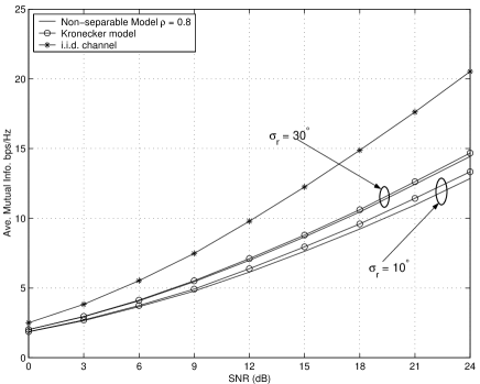
Figure 1: Average mutual information of 3-transmit UCA and 3-receive UCA MIMO system in separable (Kronecker with $\rho=0$) and non-separable $(\rho=0.8)$ scattering environments: bivariate truncated Gaussian azimuth field with mean AOD $=90^{\circ}$, mean AOA $=90^{\circ}$, transmitter angular spread $\sigma_{t}=10^{\circ}$ and receiver angular spreads $\sigma_{r}=\{30^{\circ},10^{\circ}\}$.

Figure 1 shows the average mutual information for a bivariate truncated Gaussian distributed azimuth field with $\rho=0.8$. It was shown in [16] that performance of UCA antenna configuration is less sensitive to change of mean AOD $(\phi_{0})$ and mean AOA $(\varphi_{0})$. Therefore, without loss of generality, we set $\phi_{0}=\varphi_{0}=90^{\circ}$. Also, in this simulation, we set transmitter angular spread $\sigma_{t}=10^{\circ}$ and receiver angular spreads $\sigma_{r}=\{30^{\circ},10^{\circ}\}$. For comparison, also shown is the average mutual information of the $3\times{3}$ i.i.d. MIMO channel. We observe that when $\sigma_{r}=30^{\circ}$, both models give very similar performance for all SNRs. When the angular spread at the receiver is small, e.g. $\sigma_{r}=10^{\circ}$, we can observe that the Kronecker model gives slightly higher performance than the non-separable model for higher SNRs. However, the margin of capacity over estimation is insignificant in comparison with the i.i.d. channel capacity performance. Therefore, Kronecker model provides a good estimation to the actual scattering channel when the joint scattering distribution is uni-modal. Reasoning for this claim will be discussed in the next section.

IV-A Capacity in Multi-Modal Bivariate Azimuth Fields

A multi-modal azimuth power distribution arises when there are two or more strong multipaths exist in a fading channel. This may be the result of multiple remote macroscopic scattering clusters, for instance. A multi-modal bivariate distribution can be constructed from a mixture of uni-modal bivariate distributions. Fig. 2 shows a multi-modal bivariate Gaussian distributed azimuth field with 3 modes centered around $(\phi_{0},\varphi_{0})=\{(-40^{\circ},40^{\circ}),(0^{\circ},-40^{\circ}),(50^{\circ},0^{\circ})\}$, each mode with angular spreads $\sigma_{r}=\sigma_{t}=5^{\circ}$ and $\rho=0.8$. Note that, in this case the effective angular spreads at the receiver and transmitter are larger than $5^{\circ}$.

Figure 2: An example multi-modal bivariate Gaussian distributed azimuth field.

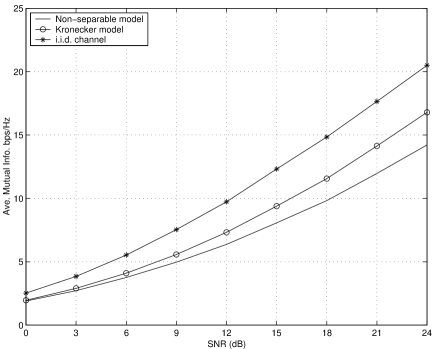
Figure 3: Average mutual information of 3-transmit UCA and 3-receive UCA MIMO system for separable and non-separable scattering channel considered in Fig. 2.

We now consider the $3{\times}3$ antenna configuration setup discussed in the previous example. Fig. 3 shows the average mutual information of it applied on the multi-modal scattering distribution shown in Fig. 2. It is observed that Kronecker model tends to overestimate the average mutual information at high SNRs. Unlike in the uni-modal case considered previously, the margin of error seen here is quite significant, especially at high SNRs. Following the analysis given in [7], we now provide reasons for Kronecker model to overestimate the mutual information for the scattering distribution shown in Fig. 4.

The joint PSD of the Kronecker model is given by $\widetilde{G}(\phi,\varphi)=\mathcal{P}_{Tx}(\phi)\mathcal{P}_{Rx}(\varphi)$, where $\mathcal{P}_{Tx}(\phi)$ and $\mathcal{P}_{Rx}(\varphi)$ are the transmit and receive power distributions, generated by marginalizing $G(\phi,\varphi)$. Fig. 4 shows the Kronecker model PSD $\widetilde{G}(\phi,\varphi)$ of the scattering channel considered in Fig. 2. Comparing Fig. 4 with Fig. 2 we can observe that $\widetilde{G}(\phi,\varphi)$ consist of six extra modes, corresponding to additional six scattering clusters. Therefore, Kronecker model introduces virtual scattering clusters located at the intersection of the actual scattering clusters. As a result, Kronecker model will increase the effective angular spread at the transmit and receive apertures (lower modal correlation) and hence improved system performance. Therefore, the popular Kronecker model does not model the MIMO channel accurately when there exist multiple scattering clusters in the channel. These observations match the measurement results published in [6].

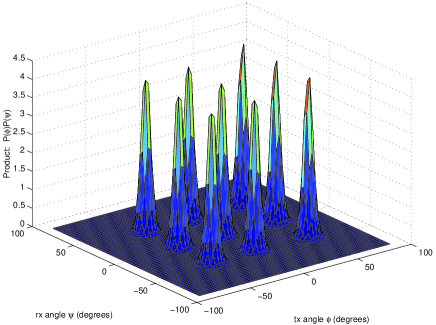
Figure 4: Kronecker model PSD $\widetilde{G}(\phi,\varphi)=\mathcal{P}_{Tx}(\phi)\mathcal{P}_{Rx}(\varphi)$ of the non-separable scattering distribution considered in Fig. 2.

Now we consider the uni-modal PSD used in our first simulation example. Fig. 5 shows the corresponding Kronecker Model PSD $\widetilde{G}(\phi,\varphi)$ for this channel, for $\sigma_{r}=10^{\circ}$ and $\sigma_{t}=10^{\circ}$. In this case the Kronecker model does not introduce any additional virtual scattering clusters into the channel. As a result, no increase in the number of multipaths of the channel, hence both models give very similar performance.

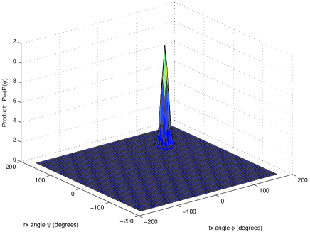
Figure 5: Kronecker model PSD $\widetilde{G}(\phi,\varphi)=\mathcal{P}_{Tx}(\phi)\mathcal{P}_{Rx}(\varphi)$ of the uni-modal non-separable scattering distribution used in the first example to obtain the results in Fig. 1 for $\sigma_{r}=10^{\circ}$.

V Conclusions

We presented a MIMO channel correlation model which is capable of capturing antenna geometry and joint correlation properties of both link ends. The scattering environment surrounding the transmitter and receiver apertures is modeled using a bi-angular power distribution. We use the covariance between transmit and receive angles to control the joint correlation properties between transmit and receive angular power distributions.

We showed that 2-D Fourier series coefficients of the bi-angular power distribution and transmit and receive antenna sampling points contribute to the entries of the correlation matrix. We proposed several bi-angular power distributions and their 2-D Fourier series coefficients in closed form.

Using the proposed model, we show that Kronecker model is a good approximation to the actual channel when the scattering channel consists of a single scattering cluster. In the presence of multiple remote scattering clusters we show that Kronecker model over estimates the performance of MIMO systems by introducing virtual scattering clusters into the channel. Therefore, in this case, Kronecker model cannot be used to represent the channel.

References

- [1] G.J. Foschini and M.J. Gans, “On limits of wireless communications in a fading environment when using multiple antennas,” Wireless Personal Communications, vol. 6, pp. 311–335, 1998.
- [2] V. Tarokh, N. Seshadri, and A.R. Calderbank, “Space-time codes for high data rate wireless communication: performance criterion and code construction,” IEEE Trans. Info. Theory, vol. 44, no. 1, pp. 744–765, Mar. 1998.
- [3] Da-Shan Shiu, G.J. Foschini, M.J. Gans, and J.M. Kahn, “Fading correlation and its effect on the capacity of multielement antenna systems,” IEEE Trans. Commun., vol. 48, no. 3, pp. 502–513, 2000.
- [4] D. Gesbert, H. Bölcskei, D.A. Gore, and A.J. Paulraj, “Outdoor MIMO wireless channels: Models and performance prediction,” IEEE Trans. Communications, vol. 50, no. 12, pp. 1926–1934, Dec. 2002.
- [5] J.P. Kermoal, L. Schumacher, K.I. Pedersen, P.E. Mogensen, and F. Frederiksen, “A stochastic MIMO radio channel model with experimental validation,” IEEE Journal on Selected Areas in Communications, vol. 20, no. 6, pp. 1211–1226, Aug. 2002.
- [6] Bonek E, H. Özxelik, M. Herdin, W. Weichselberger, and J. Wallace, “Deficiencies of a popular stochastic MIMO radio channel model,” in International Symposium on Wireless Personal Multimedia Communications (WPMC03), Yokosuka, Japan, Oct. 2003.
- [7] T.S. Pollock, “Correlation Modelling in MIMO Systems: When can we Kronecker?,” in Proc. 5th Australian Communications Theory Workshop, Newcastle, Australia, Feb. 2004, pp. 149–153.
- [8] T.D. Abhayapala, T.S. Pollock, and R.A. Kennedy, “Spatial decomposition of MIMO wireless channels,” in The Seventh International Symposium on Signal Processing and its Applications, Paris, France, July 2003, vol. 1, pp. 309–312.
- [9] T.D. Abhayapala, T.S. Pollock, and R.A. Kennedy, “Characterization of 3D spatial wireless channels,” in IEEE Vehicular Technology Conference (Fall), VTC 2003, Orlando, Florida, USA, Oct. 2003, vol. 1, pp. 123–127.
- [10] L. Hanlen and M. Fu, “Wireless communications systems with spatial diversity: a volumetric approach,” in IEEE International Conference on Communications, ICC-2003, 2003, vol. 4, pp. 2673–2677.
- [11] H.M. Jones, R.A. Kennedy, and T.D. Abhayapala, “On dimensionality of multipath fields: Spatial extent and richness,” in Proc. IEEE Int. Conf. Acoust., Speech, Signal Processing, ICASSP’2002, Orlando, Florida, May 2002, vol. 3, pp. 2837–2840.
- [12] W. Weichselberger, H. Özxelik, M. Herdin, and E. Bonek, “A novel stochastic MIMO channel model and its physical interpretation,” in 6th International Symposium on Wireless Personal Multimedia Communications (WPMC03), Yokosuka, Japan, Oct. 2003.
- [13] Johnson N. L. and Kotz S., “On some generalized farlie-gumbel-morgenstern distribution,” Communications in Statistics, vol. 4, pp. 415–427, 1975.
- [14] Lukacs E., Characteristic Functions, Hafner, New York, second edition, 1970.
- [15] Kozubowski T. J. and Podgorski K., “A multivariate and asymmetric generalization of laplace distribution,” Computational Statistics, vol. 15, no. 4, pp. 531–540, 2000.
- [16] T. A. Lamahewa, V. K. Nguyen, and T.D. Abhayapala, “Exact pairwise error probability of differential space-time codes in spatially correlated channels,” in ICC 2006, Istanbul, Turkey (submitted), pre-print : http://users.rsise.anu.edu.au/ tharaka/pubs/icc2006.pdf.