Supersymmetric extensions of Schrödinger-invariance

Malte Henkel^a and Jérémie Unterberger^b

^aLaboratoire de Physique des Matériaux, Université Henri Poincaré Nancy I,

B.P. 239, F – 54506 Vandœuvre-lès-Nancy Cedex, France

^bInstitut Elie Cartan, Université Henri Poincaré Nancy I,

B.P. 239, F – 54506 Vandœuvre-lès-Nancy Cedex, France

The set of dynamic symmetries of the scalar free Schrödinger equation in $d$ space dimensions gives a realization of the Schrödinger algebra that may be extended into a representation of the conformal algebra in $d+2$ dimensions, which yields the set of dynamic symmetries of the same equation where the mass is not viewed as a constant, but as an additional coordinate. An analogous construction also holds for the spin-${1\over 2}$ Lévy-Leblond equation. An $N=2$ supersymmetric extension of these equations leads, respectively, to a ‘super-Schrödinger’ model and to the $(3|2)$-supersymmetric model. Their dynamic supersymmetries form the Lie superalgebras ${\mathfrak{osp}}(2|2)\ltimes{\mathfrak{sh}}(2|2)$ and ${\mathfrak{osp}}(2|4)$, respectively. The Schrödinger algebra and its supersymmetric counterparts are found to be the largest finite-dimensional Lie subalgebras of a family of infinite-dimensional Lie superalgebras that are systematically constructed in a Poisson algebra setting, including the Schrödinger-Neveu-Schwarz algebra ${\mathfrak{sns}}^{(N)}$ with $N$ supercharges.

Covariant two-point functions of quasiprimary superfields are calculated for several subalgebras of ${\mathfrak{osp}}(2|4)$. If one includes both $N=2$ supercharges and time-inversions, then the sum of the scaling dimensions is restricted to a finite set of possible values.

PACS: 02.20Tw, 05.70Fh, 11.25Hf, 11.30.Pb
Keywords: conformal field-theory, correlation functions, algebraic structure of integrable models, Schrödinger-invariance, supersymmetry

1 Introduction

Symmetries have always played a central rôle in mathematics and physics. For example, it is well-known since the work of Lie (1881) that the free diffusion equation in one spatial dimension has a non-trivial symmetry group. It was recognized much later that the same group also appears to be the maximal dynamic invariance group of the free Schrödinger equation in $d$ space dimensions, and it is therefore referred to as the Schrödinger group [39]. Its Lie algebra is denoted by $\mathfrak{sch}_{d}$. In the case $d=1$, one may realize ${\mathfrak{sch}}_{1}$ by the following differential operators

$$X_{-1}=-\partial_{t}\;\;,\;\;Y_{-1/2}=-\partial_{r}$$ time and space translations

$$Y_{1/2}=-t\partial_{r}-{\cal M}r$$ Galilei transformation

$$X_{0}=-t\partial_{t}-\frac{1}{2}r\partial_{r}-\frac{x}{2}$$ dilatation

$$X_{1}=-t^{2}\partial_{t}-tr\partial_{r}-\frac{\cal M}{2}r^{2}-2xt$$ special transformation

$$M_{0}=-{\cal M}$$ phase shift (1.1)

Here, ${\cal M}$ is a (real or complex) number and $x$ is the scaling dimension of the wave function $\phi$ on which the generators of $\mathfrak{sch}_{1}$ act. The Lie algebra ${\mathfrak{sch}}_{1}$ realizes dynamical symmetries of the $1D$ free Schrödinger/diffusion equation ${\cal S}\phi=(2{\cal M}\partial_{t}-\partial_{r}^{2})\phi=0$ only if $x=1/2$.

In particular, $\mathfrak{sch}_{1}$ is isomorphic to the semi-direct product $\mathfrak{sl}_{2}(\mathbb{R})\ltimes\mathfrak{h}_{1}$, where $\mathfrak{sl}_{2}(\mathbb{R})$ is spanned by the three $X$-generators whereas the Heisenberg algebra in one space-dimension $\mathfrak{h}_{1}$ is spanned by $Y_{\pm 1/2}$ and $M_{0}$.

Schrödinger-invariance has been found in physically very different systems such as non-relativistic field-theory [30, 20, 27], celestial mechanics [12], the Eulerian equations of motion of a viscous fluid [21, 40] or the slow dynamics of statistical systems far from equilibrium [25, 42, 45], just to mention a few. In this paper, we investigate the following two important features of Schrödinger-invariance in a supersymmetric setting. The consideration of supersymmetries in relation with Schrödinger-invariance may be motivated from the long-standing topic of supersymmetric quantum mechanics [9] and from the application of Schrödinger-invariance to the long-time behaviour of systems undergoing ageing, e.g. in the context of phase-ordering kinetics. Equations such as the Fokker-Planck or Kramers equations, which are habitually used to describe non-equilibrium statistical systems, are naturally supersymmetric, see [28, 46] and references therein.

1. First, there is a certain analogy between Schrödinger- and conformal invariance. This is less surprising than it might appear at first sight since there is an embedding of the (complexified) Schrödinger Lie algebra in $d$ space dimensions into the conformal algebra in $(d+2)$ space dimensions, $\mathfrak{sch}_{d}\subset(\mathfrak{conf}_{d+2})_{\mathbb{C}}$ [7, 24]. This embedding comes out naturally when one thinks of the mass parameter $\cal M$ in the Schrödinger equation as an additional coordinate. Then a Laplace-transform of the Schrödinger equation with respect to $\cal M$ yields a Laplace-like equation which is known to be invariant under the conformal group.

2. Second, we recall the fact, observed by one of us long ago [22], that the six-dimensional Lie algebra $\mathfrak{sch}_{1}$ can be embedded into the following infinite-dimensional Lie algebra with the non-vanishing commutators

$$\left[X_{n},X_{n^{\prime}}\right] = (n-n^{\prime})X_{n+n^{\prime}}+\frac{c}{12}\left(n^{3}-n\right)\delta_{n,n^{\prime}}\;\;,\;\;\left[X_{n},Y_{m}\right]\>=\>\left(\frac{n}{2}-m\right)Y_{n+m}\;\;,\;\;$$

$$\left[X_{n},M_{n^{\prime}}\right] = -n^{\prime}M_{n+n^{\prime}}\hskip 118.07875pt\;\;,\;\;\left[Y_{m},Y_{m^{\prime}}\right]\>=\>(m-m^{\prime})M_{m+m^{\prime}}.$$ (1.2)

where $n,n^{\prime}\in\mathbb{Z}$, $m\in\mathbb{Z}+\frac{1}{2}$, and $c$ is the central charge. It can be shown that no further non-trivial central extension of this algebra is possible [22]. We shall call the algebra (1.2) the Schrödinger-Virasoro algebra and denote it by $\mathfrak{sv}$. For $c=0$, a differential-operator representation of the algebra $\mathfrak{sv}$ is

$$X_{n} = -t^{n+1}\partial_{t}-\frac{n+1}{2}\ t^{n}r\partial_{r}-(n+1)\frac{x}{2}t^{n}-\frac{n(n+1)}{4}{\cal M}t^{n-1}r^{2}$$

$$Y_{m} = -t^{m+1/2}\partial_{r}-\left(m+\frac{1}{2}\right)t^{m-1/2}r{\cal M}$$

$$M_{n} = -{\cal M}t^{n}$$ (1.3)

where $\cal M$ is a parameter and $x$ is again a scaling dimension. Extensions to higher space-dimensions are straightforward, see [23]. Remarkably, there is a ‘no-go’-theorem forbidding any reasonable double extension of the Schrödinger algebra both by the conformal algebra and by the Schrödinger-Virasoro algebra [44]. The differential equations which are conditionally invariant under the representation (1.3) of ${\mathfrak{sv}}$ with ${\cal M}=0$ are given in [8].

The algebra $\mathfrak{sv}$ can be further extended by considering the generators [23]

$$X_{n} = -t^{n+1}\partial_{t}-\frac{n+1}{2}\ t^{n}r\partial_{r}-(n+1)\frac{x}{2}t^{n}-\frac{n(n+1)}{4}{\cal M}t^{n-1}r^{2}-\frac{n^{3}-n}{8}{\cal M}^{\prime}\,t^{n-2}r^{4}$$

$$Y_{m} = -t^{m+1/2}\partial_{r}-\left(m+\frac{1}{2}\right){\cal M}t^{m-1/2}r-\left(m^{2}-\frac{1}{4}\right){\cal M}^{\prime}\,t^{m-3/2}r^{3}$$

$$Z_{n}^{(2)} = -nt^{n-1}r^{2}$$ (1.4)

$$Z_{m}^{(1)} = -2t^{m-1/2}r$$

$$Z_{n}^{(0)} = -2t^{n}$$

where $\cal M$ and ${\cal M}^{\prime}$ are (real or complex) parameters and $x$ is a scaling dimension. The non-vanishing commutators of the generators (1.4) read

$$\left[X_{n},X_{n^{\prime}}\right] = (n-n^{\prime})X_{n+n^{\prime}}\hskip 22.76228pt\;\;,\;\;\left[X_{n},Y_{m}\right]\>=\>\left(\frac{n}{2}-m\right)Y_{n+m}\;\;,\;\;$$

$$\left[Y_{m},Y_{m^{\prime}}\right] = \left(m-m^{\prime}\right)\left(48{\cal M}^{\prime}\,Z_{m+m^{\prime}}^{(2)}+\frac{\cal M}{2}Z_{m+m^{\prime}}^{(0)}\right)$$

$$\left[X_{n},Z_{n^{\prime}}^{(2)}\right] = -n^{\prime}Z_{n+n^{\prime}}^{(2)}\hskip 42.67912pt\;\;,\;\;\left[Y_{m},Z_{n}^{(2)}\right]\>=\>-nZ_{n+m}^{(1)}$$ (1.5)

$$\left[X_{n},Z_{m}^{(1)}\right] = -\left(\frac{n}{2}+m\right)Z_{n+m}^{(1)}\;\;,\;\;\left[Y_{m},Z_{m^{\prime}}^{(1)}\right]\>=\>-Z_{m+m^{\prime}}^{(0)}$$

$$\left[X_{n},Z_{n^{\prime}}^{(0)}\right] = -n^{\prime}Z_{n+n^{\prime}}^{(0)}$$

and it can be shown that for $c=0$, this is the maximal extension of $\mathfrak{sv}$ through first-order differential operators such that the time- and space- translations $X_{-1},Y_{-1/2}$ and the dilatation $X_{0}$ are unmodified compared to (1.1) [23]. For ${\cal M}^{\prime}=0$, the algebra $\mathfrak{sv}$ is recovered as a subalgebra.

Rather than proceeding from example to example, it would be valuable to have a systematic approach for the construction of infinite-dimensional (supersymmetric) extensions of $\mathfrak{sch}_{1}$.

Generalizing the correspondence between Schrödinger- and conformal invariance, we shall in this paper introduce a supersymmetric extension of the free Schrödinger equation in $d=1$ space dimension with two super-coordinates (which we call the super-Schrödinger model below), whose Lie symmetries form a supersymmetric extension of the Schrödinger algebra that is isomorphic to a semi-direct product ${\mathfrak{osp}}(2|2)\ltimes{\mathfrak{sh}}(2|2)$ of an orthosymplectic Lie algebra by a super-Heisenberg Lie algebra. We relate this model to a classical $N=2$ supersymmetric model in $(3+2)$ dimensions, giving at the same time an explicit embedding of our ‘super-Schrödinger algebra’ into ${\mathfrak{osp}}(2|4)$ . Note that supersymmetric extensions of the Schrödinger algebra have been discussed several times in the past [2, 3, 4, 15, 13, 16, 17], some of them in the context of supersymmetric quantum mechanics. Here, we consider the problem from a field-theoretical perspective.

We shall also present a systematic construction of a family of infinite-dimensional supersymmetric extensions of the Schrödinger algebra. Our main examples will be the Schrödinger-Neveu-Schwarz algebras ${\mathfrak{sns}}^{(N)}$ with $N$ supercharges. The $N=1$ Neveu-Schwarz superalgebra [38, 29] is recovered as a subalgebra of ${\mathfrak{sns}}^{(1)}$, while ${\mathfrak{sns}}^{(0)}$ is the Schrödinger-Virasoro algebra ${\mathfrak{sv}}$.

The link between the two parts is given by a realization of the infinite-dimensional Lie algebra ${\mathfrak{sns}}^{(2)}$ providing an extension of the realization of ${\mathfrak{osp}}(2|2)\ltimes{\mathfrak{sh}}(2|2)$ as Lie symmetries of the super-Schrödinger model (see Proposition 4.3).

We begin in section 2 by recalling some useful facts about the Schrödinger-invariance of the scalar free Schrödinger equation and then give a generalization to its spin-${1\over 2}$ analogue, the Lévy-Leblond equation. By considering the ‘mass’ as an additional variable, we extend the spinor representation of the Schrödinger algebra ${\mathfrak{sch}}_{1}$ into a representation of ${\mathfrak{conf}}_{3}$. As an application, we derive the Schrödinger-covariant two-point spinorial correlation functions. In section 3, we combine the free Schrödinger and Lévy-Leblond equations (together with a scalar auxiliary field) into a super-Schrödinger model, and show, by using a superfield formalism in $3+2$ dimensions, that this model has a kinematic supersymmetry algebra with $N=2$ supercharges. Including then time-inversions, we compute the full dynamical symmetry algebra and prove that it is isomorphic to the Lie algebra of symmetries ${\mathfrak{osp}}(2|2)\ltimes{\mathfrak{sh}}(2|2)$ found in several mechanical systems with a finite number of particles. By treating the ‘mass’ as a coordinate, we obtain a well-known supersymmetric model (see [14]) that we call the $(3|2)$-supersymmetric model. Its dynamical symmetries form the Lie superalgebra ${\mathfrak{osp}}(2|4)$. The derivation of these results is greatly simplified through the correspondence with Poisson structures and the introduction of several gradings which will be described in detail. In section 4, we use a Poisson algebra formalism to construct for every $N$ an infinite-dimensional supersymmetric extension with $N$ supercharges of the Schrödinger algebra that we call Schrödinger-Neveu-Schwarz algebra and denote by ${\mathfrak{sns}}^{(N)}$. At the same time, we give an extension of the differential-operator representation of ${\mathfrak{osp}}(2|4)$ into a differential-operator representation of ${\mathfrak{sns}}^{(2)}$. We compute in section 5 the two-point correlation functions that are covariant under ${\mathfrak{osp}}(2|4)$ or under some of its subalgebras. Remarkably, in many instances, the requirement of supersymmetric covariance is enough to allow only a finite number of possible quasiprimary superfields. Our conclusions are given in section 6. In appendix A we present the details for the calculation of the supersymmetric two-point functions, whereas in appendix B, we collect for easy reference the numerous Lie superalgebras introduced in the paper and their differential-operator realization as Lie symmetries of the $(3|2)$-supersymmetric model.

2 On the Dirac-Lévy-Leblond equation

Throughout this paper we shall use the following notation: $[A,B]_{\mp}:=AB\mp BA$ stand for the commutator and anticommutator, respectively. We shall often simply write $[A,B]$ if it is clear which one should be understood. Furthermore $\{A,B\}:={\partial A\over\partial q}\ {\partial B\over\partial p}-{\partial A\over\partial p}\ {\partial B\over\partial q}$ denotes the Poisson bracket or supersymmetric extensions thereof which will be introduced below. We shall use the Einstein summation convention unless explicitly stated otherwise.

In this section we first recall some properties of the one-dimensional free Schrödinger equation before considering a reduction to a system of first-order equations introduced by Lévy-Leblond [35].

Figure 1: Roots of the three-dimensional complexified conformal Lie algebra $(\mathfrak{conf}_{3})_{\mathbb{C}}\cong B_{2}$ and their relation with the generators of the Schrödinger algebra $\mathfrak{sch}_{1}$. The double circle in the centre denotes the Cartan subalgebra $\mathfrak{h}$.

Consider the free Schrödinger or diffusion equation

$${\cal S}\tilde{\phi}=(2{\cal M}\partial_{t}-\partial_{r}^{2})\tilde{\phi}=0$$ (2.1)

in one space-dimension, where the Schrödinger operator may be expressed in terms of the generators of $\mathfrak{sch}_{1}$ as ${\cal S}:=2M_{0}X_{-1}-{Y}_{-1/2}^{2}$. That the Schrödinger algebra realized by (1.1) is indeed a dynamical symmetry of the Schrödinger equation if $x=1/2$ can be seen from the commutators

$${}\left[{\cal S},X_{1}\right]=-2t{\cal S}-2\left(x-\frac{1}{2}\right)M_{0}\;\;,\;\;{}\left[{\cal S},X_{-1}\right]=\left[{\cal S},Y_{-{1\over 2}}\right]=0$$ (2.2)

while the symmetry with respect to the other generators follows from the Jacobi identities. In many situations, it is useful to go over from the representation eq. (1.1) to another one obtained by formally considering the ‘mass’ ${\cal M}$ as an additional variable such that $\tilde{\phi}=\tilde{\phi}_{\cal M}(t,r)$. As a general rule, we shall denote in this article by $\zeta$ the variable conjugate to $\cal M$ via a Fourier-Laplace transformation, and the corresponding wave function by the same letter but without the tilde, here $\phi=\phi(\zeta,t,r)$. In this way, one may show that there is a complex embedding of the Schrödinger algebra into the conformal algebra, viz. $(\mathfrak{sch}_{1})_{\mathbb{C}}\subset(\mathfrak{conf}_{3})_{\mathbb{C}}$ [24], whereas the representation (1.1) (after a Fourier-Laplace transform) may be extended into the usual representation of ${\mathfrak{conf}}_{3}$ as infinitesimal conformal transformations of $\mathbb{R}^{3}$ for a certain choice of coordinates.

We illustrate this for the one-dimensional case $d=1$ in figure 1, where the root diagram for $(\mathfrak{conf}_{3})_{\mathbb{C}}\cong B_{2}$ is shown. The identification with the generators of $\mathfrak{sch}_{1}$ is clear, see eq. (1.1), and we also give a name to the extra conformal generators. In particular, $\langle N,X_{0}\rangle$ form a Cartan subalgebra and the eigenvalue of ${\mathrm{ad\,}}N$ on any root vector is given by the coordinate along $-e_{1}$. Furthermore, the conformal invariance of the Schrödinger equation follows from $[{\cal S},V_{-}]=0$ [24].

One of the main applications of the (super-)symmetries studied in this article will be the calculation of covariant correlation functions and we now define this important concept precisely, generalizing a basic concept of conformal field-theory [5].

Definition 1. Let ${\cal L}({\cal H})$ be the set of linear operators on a Hilbert space $\cal H$, let $R:\mathfrak{g}\to{\cal L}({\cal H})$ be a representation of a (super) Lie algebra $\mathfrak{g}$ and $R^{(n)}:\mathfrak{g}\to{\cal L}({\cal H})^{\otimes n}$ be the tensor representation for $n$-particle operators. If $\phi_{1},\ldots,\phi_{n}\in{\cal H}$ are fields, then their $n$-point function $\langle\phi_{1}\ldots\phi_{n}\rangle$ may be defined by an averaging function $\mathrm{Av}:{\cal H}^{\otimes n}\to\mathbb{C}$ such that $\mathrm{Av\,}(\phi_{1}\otimes\ldots\otimes\phi_{n})=\langle\phi_{1}\ldots\phi_{n}\rangle$. Then one says that the $n$-point function $\langle\phi_{1}\cdots\phi_{n}\rangle$ is $\mathfrak{g}$-covariant under the representation $R$, if for any generator ${\cal X}\in\mathfrak{g}$

$${\mathrm{Av}}\left(R^{(n)}({\cal X})(\phi_{1}\otimes\ldots\phi_{n})\right)=\langle({\cal R}({\cal X})\phi_{1})\phi_{2}\ldots\phi_{n}\rangle+\ldots+\langle\phi_{1}\ldots\phi_{n-1}({\cal R}({\cal X})\phi_{n})\rangle=0$$ (2.3)

In this case, the fields $\phi_{i}$ are called $\mathfrak{g}$-quasiprimary with respect to $R$, or simply quasiprimary.

As a specific example, let us consider here $n$-point functions that are covariant under $(\mathfrak{conf}_{3})_{\mathbb{C}}$ or one of its Lie subalgebras, which for our purposes will be either $\mathfrak{sch}_{1}$ or the parabolic subalgebra

$$\widetilde{{\mathfrak{sch}}}_{1}:=\mathbb{C}N\ltimes{\mathfrak{sch}}_{1}$$ (2.4)

(see [31] for the definition of parabolic subalgebras). In the extension of the Fourier-Laplace transform of the representation (1.1) to ${\mathfrak{conf}}_{3}$, the generator $N$ is given by

$$N=-t\partial_{t}+\zeta\partial_{\zeta}+\nu$$ (2.5)

with $\nu=0$ [24]. But any choice for the value of $\nu$ also gives a representation of $\widetilde{{\mathfrak{sch}}}_{1}$, although it does not extend to the whole conformal Lie algebra. So one may consider more generally $\widetilde{{\mathfrak{sch}}}_{1}$-quasiprimary fields characterized by a scaling exponent $x$ and a $N$-exponent $\nu$.

It will turn out later to be useful to work with the variable $\zeta$ conjugate to $\cal M$. If we arrange for ${\cal M}=-{1\over 2}\partial_{\zeta}$ through a Laplace transform, see eq. (2.11) below, it is easy to see that the ${\mathfrak{sch}}_{1}$-covariant two-point function under the representation (1.1) is given by [24]

$$\left\langle\phi_{1}\phi_{2}\right\rangle:=\left\langle\phi_{1}(\zeta_{1},t_{1},r_{1})\phi_{2}(\zeta_{2},t_{2},r_{2})\right\rangle=\psi_{0}\delta_{x_{1},x_{2}}(t_{1}-t_{2})^{-x_{1}}f\left(\zeta_{1}-\zeta_{2}+\frac{1}{4}\frac{(r_{1}-r_{2})^{2}}{t_{1}-t_{2}}\right)$$ (2.6)

where $x_{1,2}$ are the scaling dimensions of the ${\mathfrak{sch}}_{1}$-quasiprimary fields $\phi_{1,2}$, $f$ is an undetermined scaling function and $\psi_{0}$ a normalization constant. If $\phi_{1,2}$ are $\widetilde{{\mathfrak{sch}}}_{1}$-quasiprimary fields with $N$-exponents $\nu_{1,2}$, then $f(u)=u^{-x_{1}-\nu_{1}-\nu_{2}}$. If in addition $\psi_{1,2}$ are $\mathfrak{conf}_{3}$-quasiprimary, then $f(u)=u^{-x_{1}}$ and, after an inverse Laplace transform, this two-point function becomes the well-known heat kernel $\langle\tilde{\phi}_{1}\tilde{\phi}_{2}\rangle=\phi_{0}\delta_{x_{1},x_{2}}t^{-x_{1}}\exp(-r^{2}/(2{\cal M}t))$, together with the causality condition $t>0$ [24]. The same form for $\langle\tilde{\phi}_{1}\tilde{\phi}_{2}\rangle$ also holds true for ${\mathfrak{sch}}_{1}$-quasiprimary fields, since the function $f$ in (2.6) simply gives, after the Laplace transform, a mass-dependent normalization constant $\phi_{0}$.

We now turn to the Dirac-Lévy-Leblond equations. They were constructed by Lévy-Leblond [35] by adapting to a non-relativistic setting Dirac’s square-root method for finding a relativistically covariant partial differential equation of first order. Consider in $d$ space dimensions a first-order vector wave equation of the form

$${\cal R}\tilde{\Phi}:=\left(A\frac{\partial}{\partial t}+\sum_{i=1}^{d}B_{i}\frac{\partial}{\partial r^{i}}+{\cal M}C\right)\tilde{\Phi}=0$$ (2.7)

where $A,B_{i}$ and $C$ are matrices to be determined such that the square of the operator $\cal R$ is equal to the free Schrödinger operator ${\cal R}^{2}\stackrel{{\scriptstyle!}}{{=}}{\cal S}=2{\cal M}\partial_{t}-\sum_{i=1}^{d}({\partial_{r^{i}}})^{2}$. It is easy to see that the matrices $A,B_{i},C$ give a representation of a Clifford algebra (with an unconventional metric) in $d+2$ dimensions. Namely, if one sets

$$\mathfrak{B}_{j} := {\rm i}\sqrt{2\,}B_{j}\;\;;\;\;j=1,\ldots,d$$

$$\mathfrak{B}_{d+1} := A+\frac{1}{2}C\;\;,\;\;\mathfrak{B}_{d+2}\>:=\>{\rm i}\left(A-\frac{1}{2}C\right)$$ (2.8)

then the condition on ${\cal R}$ is equivalent to $[\mathfrak{B}_{j},\mathfrak{B}_{k}]_{+}=2\delta_{j,k}$ for $j,k=1,\ldots,d+2$.

We are interested in the case $d=1$. Then the Clifford algebra generated by $\mathfrak{B}_{j}$, $j=1,2,3$, has exactly one irreducible representation up to equivalence, which is given for instance by

$$\mathfrak{B}_{1}=\sigma^{3}=\left(\begin{array}[]{cc}1&0\\ 0&-1\end{array}\right)\;\;,\;\;\mathfrak{B}_{2}=\sigma^{2}=\left(\begin{array}[]{cc}0&{\rm i}\\ -{\rm i}&0\end{array}\right)\;\;,\;\;\mathfrak{B}_{3}=\sigma^{1}=\left(\begin{array}[]{cc}0&1\\ 1&0\end{array}\right).$$ (2.9)

Then the wave equation ${\cal R}\tilde{\Phi}={\cal R}\left(\begin{array}[]{cc}\tilde{\psi}\\ \tilde{\phi}\end{array}\right)=0$ becomes explicitly, after a rescaling $r\mapsto\sqrt{2\,}r$

$$\partial_{t}\tilde{\psi}=\partial_{r}\tilde{\phi}\;\;,\;\;2{\cal M}\tilde{\phi}=\partial_{r}\tilde{\psi}$$ (2.10)

These are the Dirac-Lévy-Leblond equations in one space dimension.

Since the masses $\cal M$ are by physical convention real and positive, it is convenient to define their conjugate $\zeta$ through a Laplace transform

$${\psi}(\zeta,t,r)=\int_{0}^{\infty}\!{\rm d}{\cal M}\>e^{-2{\cal M}\zeta}\tilde{\psi}({\cal M};t,r)$$ (2.11)

and similarly for $\phi$. Then eqs. (2.10) become

$$\partial_{t}{\psi}=\partial_{r}{\phi}\;\;,\;\;\partial_{\zeta}{\phi}=-\partial_{r}{\psi}.$$ (2.12)

Actually, it is easy to see that these eqs. (2.12) are equivalent to the three-dimensional massless free Dirac equation $\gamma^{\mu}\partial_{\mu}\Phi=0$, where $\partial_{\mu}=\partial/\partial\xi^{\mu}$ and $\xi^{\mu}$ with $\mu=1,2,3$ are the coordinates. If we set $t={1\over 2}(\xi^{1}+{\rm i}\xi^{2})$, $\zeta={1\over 2}(\xi^{1}-{\rm i}\xi^{2})$ and finally $r=\xi^{3}$, and choose the representation $\gamma^{\mu}=\sigma^{\mu}$, then we recover indeed eq. (2.12).

The invariance of the free massless Dirac equation under the conformal group is well-known. The generators of $\mathfrak{conf}_{3}$ act as follows on the spinor field $\Phi=\left(\begin{array}[]{c}\psi\\ \phi\end{array}\right)$, (see again figure 1)

$$X_{-1} = -\partial_{t}\;\;,\;\;Y_{-{1\over 2}}\>=\>-\partial_{r}\;\;,\;\;M_{0}\>=\>{1\over 2}\partial_{\zeta}$$

$$V_{-} = -r\partial_{t}+2\zeta\partial_{r}-\left(\begin{array}[]{cc}0&1\\ 0&0\end{array}\right)$$ (2.15)

$$N = -t\partial_{t}+\zeta\partial_{\zeta}+{1\over 2}\left(\begin{array}[]{cc}1&0\\ 0&-1\end{array}\right)$$ (2.18)

$$Y_{{1\over 2}} = -t\partial_{r}+{1\over 2}r\partial_{\zeta}-{1\over 2}\left(\begin{array}[]{cc}0&0\\ 1&0\end{array}\right)$$ (2.21)

$$X_{0} = -t\partial_{t}-{1\over 2}r\partial_{r}-{1\over 2}\left(\begin{array}[]{cc}x&0\\ 0&x+1\end{array}\right)$$ (2.24)

$$W = -{1\over 2}r^{2}\partial_{t}+2\zeta^{2}\partial_{\zeta}+2\zeta r\partial_{r}+\left(\begin{array}[]{cc}2(x+1)\zeta&-r\\ 0&2x\zeta\end{array}\right)$$ (2.27)

$$V_{+} = -tr\partial_{t}-\zeta r\partial_{\zeta}-{1\over 2}(r^{2}-4\zeta t)\partial_{r}-{1\over 2}\left(\begin{array}[]{cc}(2x+1)r&2t\\ -2\zeta&(2x+1)r\end{array}\right)$$ (2.30)

$$X_{1} = -t^{2}\partial_{t}-tr\partial_{r}+\frac{1}{4}r^{2}\partial_{\zeta}-\left(\begin{array}[]{cc}xt&0\\ r/2&(x+1)t\end{array}\right)$$ (2.33)

For solutions of (2.12), one has $x={1\over 2}$. As in the case of the scalar representation (1.1), arbitrary values of the scaling exponent $x$ also give a representation of the conformal algebra.

There are three ‘translations’ ($X_{-1},Y_{-{1\over 2}},M_{0}$), three ‘rotations’ ($V_{-},N,Y_{{1\over 2}}$), one ‘dilatation’ ($X_{0}$) and three ‘inversions’ or special transformations ($W,V_{+},X_{1}$). It is sometimes useful to work with the generator $D:=2X_{0}-N$ (whose differential part is the Euler operator $-t\partial_{t}-r\partial_{r}-\zeta\partial_{\zeta}$) instead of either $X_{0}$ or $N$. We also see that the individual components $\psi,\phi$ of the spinor $\Phi$ have scaling dimensions $x_{\psi}=x$ and $x_{\phi}=x+1$, respectively. If we write the Dirac operator as

$${\cal D}=\frac{1}{{\rm i}}{\cal R}=\left(\begin{array}[]{cc}\partial_{r}&\partial_{\zeta}\\ \partial_{t}&-\partial_{r}\end{array}\right)$$ (2.34)

then the Schrödinger- and also the full conformal invariance of the Dirac-Lévy-Leblond equation ${\cal D}\Phi=0$ follows from the commutators

$${}\left[{\cal D},X_{1}\right] = -t{\cal D}-\left(x-{1\over 2}\right)\left(\begin{array}[]{cc}0&0\\ 0&1\end{array}\right)$$ (2.37)

$${}\left[{\cal D},X_{-1}\right] = \left[{\cal D},Y_{-{1\over 2}}\right]\>=\>\left[{\cal D},V_{-}\right]\>=\>0$$ (2.38)

It is clear that dynamical symmetries of the Dirac-Lévy-Leblond equation are obtained only if $x={1\over 2}$. Since $X_{1},X_{-1},Y_{-{1\over 2}},V_{-}$ generate $(\mathfrak{conf}_{3})_{\mathbb{C}}$, as can be seen from the root structure represented in figure 1, the symmetry under the remaining generators of $(\mathfrak{conf}_{3})_{\mathbb{C}}$ follows from the Jacobi identities.

Let $\Phi_{i}=\left(\mbox{${\begin{array}[]{c}\psi_{i}\\ \phi_{i}\end{array}}$}\right)$ , $i=1,2$ be two quasiprimary spinors under the representation (2.24) of either ${\mathfrak{sch}}_{1},\widetilde{{\mathfrak{sch}}}_{1}$ or ${\mathfrak{conf}}_{3}$, with scaling dimensions $\left(\mbox{${\begin{array}[]{c}x_{i}\\ x_{i}+1\end{array}}$}\right)$ of the component fields. We now consider the covariant two-point functions; from translation-invariance it is clear that these will only depend on $\zeta=\zeta_{1}-\zeta_{2}$, $t=t_{1}-t_{2}$ and $r=r_{1}-r_{2}$.

Proposition 2.1. Suppose $\Phi_{1}$, $\Phi_{2}$ are quasiprimary spinors under the representation (2.24) of $\widetilde{{\mathfrak{sch}}}_{1}$. Then their two-point functions vanish unless $x_{1}=x_{2}$ or $x_{1}=x_{2}\pm 1$, in which case they read ($\phi_{0},\psi_{0}$ are normalization constants)

(i) if $x_{1}=x_{2}$, then

$$\langle\psi_{1}\psi_{2}\rangle = \psi_{0}t\left(4\zeta t+r^{2}\right)^{-x_{1}-1}$$

$$\langle\psi_{1}\phi_{2}\rangle = \langle\phi_{1}\psi_{2}\rangle\>=\>-{1\over 2}\psi_{0}r\left(4\zeta t+r^{2}\right)^{-x_{1}-1}$$ (2.39)

$$\langle\phi_{1}\phi_{2}\rangle = \frac{\psi_{0}}{4}\frac{r^{2}}{t}\left(4\zeta t+r^{2}\right)^{-x_{1}-1}+\phi_{0}\frac{1}{t}\left(4\zeta t+r^{2}\right)^{-x_{1}}$$

(ii) if $x_{1}=x_{2}+1$, then

$$\langle\psi_{1}\psi_{2}\rangle = \langle\phi_{1}\psi_{2}\rangle\>=\>0$$

$$\langle\psi_{1}\phi_{2}\rangle = \psi_{0}\left(4\zeta t+r^{2}\right)^{-x_{1}}$$ (2.40)

$$\langle\phi_{1}\phi_{2}\rangle = -\frac{\psi_{0}}{2}\frac{r}{t}\left(4\zeta t+r^{2}\right)^{-x_{1}}$$

The case $x_{1}=x_{2}-1$ is obtained by exchanging $\Phi_{1}$ with $\Phi_{2}$.

For brevity, the arguments of the two-point functions in eqs. (2.39,2.40) were suppressed. Let us emphasize that the scaling dimensions of the component fields with a standard Schrödinger form eq. (2.6) ($\langle\psi_{1}\psi_{2}\rangle$ and $\langle\phi_{1}\phi_{2}\rangle$ in eq. (2.39), and $\langle\psi_{1}\phi_{2}\rangle$ in eq. (2.40)) must agree, which is not the case for the other two-point functions which are obtained from them by applying derivative operators.

On the other hand, the covariance under the whole conformal group implies the supplementary constraint $x_{1}=x_{2}$ (equality of the scaling exponents), and we have

Proposition 2.2. The non-vanishing two-point functions, $(\mathfrak{conf}_{3})_{\mathbb{C}}$-covariant under the representation (2.24), of the fields $\psi$ and $\phi$ are obtained from eq. (2.39) with $x_{1}=x_{2}$ and the extra condition $\phi_{0}=-\psi_{0}/4$, which gives

$$\langle\phi_{1}\phi_{2}\rangle=-\psi_{0}\zeta\left(4\zeta t+r^{2}\right)^{-x_{1}-1}$$ (2.41)

Proof: In proving these two propositions, we merely outline the main ideas since the calculations are straightforward. We begin with Proposition 2.1. Given the obvious invariance under the translations, we first consider the invariance under the special transformation $X_{1}$ and use the form (2.24). With the help of dilatation invariance ($X_{0}$) and Galilei-invariance ($Y_{{1\over 2}}$) this simplifies to

$$(x_{1}-x_{2})t\langle\psi_{1}\psi_{2}\rangle = 0\;\;,\;\;(x_{1}-x_{2}-1)t\langle\psi_{1}\phi_{2}\rangle-{1\over 2}r\langle\psi_{1}\psi_{2}\rangle\>=\>0\;\;,\;\;$$

$$(x_{1}-x_{2}+1)t\langle\phi_{1}\psi_{2}\rangle+{1\over 2}r\langle\psi_{1}\psi_{2}\rangle = 0\;\;,\;\;(x_{1}-x_{2})t\langle\phi_{1}\phi_{2}\rangle+{1\over 2}r\langle\psi_{1}\phi_{2}\rangle-{1\over 2}r\langle\phi_{1}\psi_{2}\rangle\>=\>0$$

Considering the first of these equations leads us to distinguish two cases: either (i) $x_{1}=x_{2}$ or (ii) $\langle\psi_{1}\psi_{2}\rangle=0$.

In the first case, we get from the remaining three equations

$$\langle\psi_{1}\phi_{2}\rangle=\langle\phi_{1}\psi_{2}\rangle=-\frac{r}{2t}\langle\psi_{1}\psi_{2}\rangle$$

and the covariance under $Y_{{1\over 2}}$, $N$ and $X_{0}$, respectively, leads to the following system of equations

$$\left(-t\frac{\partial}{\partial r}+\frac{r}{2}\frac{\partial}{\partial\zeta}\right)\langle\psi_{1}\psi_{2}\rangle = 0\;\;,\;\;\left(-t\frac{\partial}{\partial t}+\zeta\frac{\partial}{\partial\zeta}+1\right)\langle\psi_{1}\psi_{2}\rangle\>=\>0\;\;,\;\;$$

$$\left(-t\frac{\partial}{\partial t}-\frac{r}{2}\frac{\partial}{\partial r}-x_{1}\right)\langle\psi_{1}\psi_{2}\rangle = 0$$

with a unique solution (up to a multiplicative factor) given by the first line of eq. (2.39). Similarly, covariance under the same three generators leads to a system of three linear inhomogeneous equations for $\langle\phi_{1}\phi_{2}\rangle$ whose general solution is also given in eq. (2.39).

In the second case, the remaining conditions coming from $X_{1}$ are

$$(x_{1}-x_{2}-1)t\langle\psi_{1}\phi_{2}\rangle\>=\>0\;\;,\;\;(x_{1}-x_{2}+1)t\langle\phi_{1}\psi_{2}\rangle = 0\;\;,\;\;$$

$$(x_{1}-x_{2})t\langle\phi_{1}\phi_{2}\rangle+\frac{r}{2}\left(\langle\psi_{1}\phi_{2}\rangle-\langle\phi_{1}\psi_{2}\rangle\right) = 0$$

and one of the conditions $x_{1}=x_{2}\pm 1$ must hold true. Supposing that $x_{1}=x_{2}+1$, we get $\langle\phi_{1}\phi_{2}\rangle=-{1\over 2}(r/t)\langle\psi_{1}\phi_{2}\rangle$ and an analogous relation holds (with the first and second field exchanged) in the other case. Again, covariance under $Y_{{1\over 2}},N,X_{0}$ leads to a system of three linear equations for $\langle\psi_{1}\phi_{2}\rangle$ whose general solution in given in eq. (2.40).

To prove Proposition 2.2, it is now sufficient to verify covariance under the generator $V_{-}$. Direct calculation shows that eq. (2.39) is compatible with this condition only if $\phi_{0}=-\psi_{0}/4$. On the other hand, compatibility with the second case eq. (2.40) requires that $\psi_{0}=0$. $\Box$

Remark: If we come back to the original fields $\tilde{\psi},\tilde{\phi}$ by inverting the Laplace transform (2.11), the $\widetilde{{\mathfrak{sch}}}_{1}$-covariant two-point functions of eq. (2.39) take the form

$$\langle\tilde{\psi}_{1}\tilde{\psi}_{2}\rangle = \psi_{0}^{\prime}\left(\frac{\cal M}{t}\right)^{x_{1}}\exp\left(-\frac{{\cal M}}{2}\frac{r^{2}}{t}\right)$$

$$\langle\tilde{\psi}_{1}\tilde{\phi}_{2}\rangle = \langle\tilde{\phi}_{1}\tilde{\psi}_{2}\rangle\>=\>-\psi_{0}^{\prime}\frac{r}{2t}\left(\frac{\cal M}{t}\right)^{x_{1}}\exp\left(-\frac{{\cal M}}{2}\frac{r^{2}}{t}\right)$$ (2.42)

$$\langle\tilde{\phi}_{1}\tilde{\phi}_{2}\rangle = \frac{\psi_{0}^{\prime}}{4}\frac{r^{2}}{t}\left(\frac{\cal M}{t}\right)^{x_{1}}\exp\left(-\frac{{\cal M}}{2}\frac{r^{2}}{t}\right)+\phi_{0}^{\prime}\left(\frac{\cal M}{t}\right)^{x_{1}-1}\exp\left(-\frac{{\cal M}}{2}\frac{r^{2}}{t}\right)$$

where $\psi_{0}^{\prime}=\psi_{0}/(\Gamma(x_{1}+1)2^{x_{1}+1})$, $\phi_{0}^{\prime}=\phi_{0}/(\Gamma(x)2^{x_{1}})$, and $\Gamma(x)$ is the Gamma function.

Proposition 2.3. (i) Let $f$ be a solution of the Laplace-transformed Schrödinger equation $(\partial_{\zeta}\partial_{t}+\partial_{r}^{2})f=0$. Then $\Phi=\left(\mbox{${\begin{array}[]{c}\psi\\ \phi\end{array}}$}\right):=\left(\begin{array}[]{c}-\partial_{\zeta}f\\ \partial_{r}f\end{array}\right)$ satisfies the Dirac-Lévy-Leblond equations (2.12).
(ii) Suppose that $f_{1},f_{2}$ are $\widetilde{{\mathfrak{sch}}}_{1}$-quasiprimary fields with scaling exponents $x=x_{1}=x_{2}$ and $N$-exponents $\nu_{1}=\nu_{2}=-{1\over 2}$, and let $\Phi_{i}:=\left(\begin{array}[]{c}-\partial_{\zeta}f_{i}\\ \partial_{r}f_{i}\end{array}\right)$. Then the covariant two-point function

$$\langle f_{1}f_{2}\rangle=t^{-x}(\zeta+r^{2}/4t)^{1-x}$$

implies a particular case of eq. (2.39), given by $\psi_{0}=-x(x-1)2^{2x+2}$ and $\phi_{0}=(x-1)2^{2x-1}$.

Both assertions are easily checked by straightforward calculations.

Remark: In the case (i) of Proposition 2.3, the correspondence $\Phi_{i}=\left(\mbox{${\begin{array}[]{c}\psi_{i}\\ \phi_{i}\end{array}}$}\right)=\left(\mbox{${\begin{array}[]{c}-\partial_{\zeta}f_{i}\\ \partial_{r}f_{i}\end{array}}$}\right)$ induces from (1.1) a representation of the Schrödinger group on the fields $\phi_{i},\psi_{i}$ in terms of integro-differential operators. It is at first sight not obvious that the two-point function of spinors that are quasiprimary under (2.24) should be derived from $\langle f_{1}f_{2}\rangle$ in such a simple way.

3 Supersymmetry in three dimensions and supersymmetric Schrödinger-invariance

3.1 From $N=2$ supersymmetry to the super-Schrödinger equation

We begin by recalling the construction of super space-time [14, Lectures 3 & 4]. Take as $n$-dimensional space-time $\mathbb{R}^{n}$ (or, more generally, any $n$-dimensional Lorentzian manifold). One has a quite general construction of (non-supercommutative) superspace-time $\mathbb{R}^{n|s}$, with $s$ odd coordinates, as the exponential of the Lie superalgebra $V\oplus S$, where the even part $V$ is an $n$-dimensional vector space, and the $s$-dimensional odd part $S$ is a spin representation of dimension $s$ of Spin$(n-1,1)$, provided with non-trivial Lie super-brackets $(f_{1},f_{2})\in S\times S\mapsto[f_{1},f_{2}]_{+}\in V$ which define a Spin$(n-1,1)$-equivariant pairing $\Gamma:{\rm Sym}^{2}(S)\to V$ from symmetric two-tensors on $S$ into $V$ (see [14], Lecture 3). Super-spacetime $\mathbb{R}^{n|s}$ can then be extended in a natural way into the exponential of the super-Poincaré algebra $({\mathfrak{spin}}(n-1,1)\ltimes V)\oplus S$, with the canonical action of ${\mathfrak{spin}}(n-1,1)$ on $V$ and on $S$.

Let us make this construction explicit in space-time dimension $n=3$, which is the only case that we shall study in this paper. Then the minimal spin representation is two-dimensional, so we consider super-spacetime $\mathbb{R}^{3|2}$ with two odd coordinates $\theta=(\theta^{1},\theta^{2})$. We shall denote by $D_{\theta^{a}}$, $a=1,2$, the associated left-invariant derivatives, namely, the left-invariant super-vector fields that coincide with $\partial_{\theta^{1}},\partial_{\theta^{2}}$ when $\theta^{1},\theta^{2}\equiv 0$. Consider $\mathbb{R}^{2}$ with the coordinate vector fields $\partial_{y^{1}},\partial_{y^{2}}$ and the associated symmetric two-tensors with components $\partial_{y^{ij}}$, $i,j=1,2$. These form a three-dimensional vector space with natural coordinates $y=(y^{11},y^{12},y^{22})$ defined by

$$\left[\partial_{y^{cd}},y^{ab}\right]_{-}:=\delta_{ca}\delta_{db}+\delta_{cb}\delta_{da}$$ (3.1)

Then define the map $\Gamma$ introduced above to be

$$\Gamma(\partial_{\theta^{a}},\partial_{\theta^{b}}):=\partial_{y^{ab}}$$ (3.2)

Hence, one has the simple relation $[D_{\theta^{a}},D_{\theta^{b}}]_{+}=\partial/\partial y^{ab}$ for the odd generators of $\mathbb{R}^{3|2}$. So, by the Campbell-Hausdorff formula,

$$D_{\theta^{a}}=\partial_{\theta^{a}}+\theta^{b}\partial_{y^{ab}}.$$ (3.3)

In this particular case, ${\mathfrak{spin}}(2,1)\cong{\mathfrak{sl}}(2,\mathbb{R})$. The usual action of ${\mathfrak{gl}}(2,\mathbb{R})\supset{\mathfrak{spin}}(2,1)$ on $\mathbb{R}^{2}$ is given by the two-by-two matrices $E_{ab}$ such that $E_{ab}\partial_{y^{c}}=-\delta_{ac}\partial_{y^{b}}$ and extends naturally to the following action on symmetric 2-tensors

$$E_{ab}\partial_{y^{cd}}=-\delta_{ac}\partial_{y^{bd}}-\delta_{ad}\partial_{y^{cb}}\>=\>\left[y^{a\bar{a}}\partial_{y^{\bar{a}b}},\partial_{y^{cd}}\right]_{-},$$ (3.4)

so $E_{ab}$ is represented by the vector field on $V\oplus S$

$$E_{ab}=y^{a\bar{a}}\partial_{y^{\bar{a}b}}+\theta^{a}\partial_{\theta^{b}}$$ (3.5)

One may verify that the adjoint action of $E_{ab}$ on the left-covariant derivatives is given by the usual matrix action, namely, $[E_{ab},D_{\theta^{c}}]=-\delta_{ac}D_{\theta^{b}}$.

Consider now a superfield $\Phi(y^{11},y^{12},y^{22};\theta^{1},\theta^{2})$: we introduce the Lagrangian density

$${\cal L}(\Phi)={1\over 2}\varepsilon^{ab}(D_{\theta^{a}}\Phi)^{*}(D_{\theta^{b}}\Phi)$$ (3.6)

where $\varepsilon^{ab}$ is the totally antisymmetric two-tensor defined by $\varepsilon^{12}=-\varepsilon^{21}=1,\ \varepsilon^{11}=\varepsilon^{22}=0.$ It yields the equations of motion

$$\varepsilon^{ab}D_{\theta^{a}}D_{\theta^{b}}\Phi=(D_{\theta^{1}}D_{\theta^{2}}-D_{\theta^{2}}D_{\theta^{1}})\Phi=0.$$ (3.7)

This equation is invariant under even translations $\partial_{y^{ab}}$, and under right-invariant super-derivatives

$$\bar{D}_{\theta^{a}}=\partial_{\theta^{a}}-\theta^{b}\partial_{y^{ab}}$$ (3.8)

since these anticommute with the $D_{\theta^{a}}$. Furthermore, the Lagrangian density is multiplied by $\det(g)$ under the action of $g\in{\mathrm{Gl}}(2,\mathbb{R})$, hence all elements in ${\mathfrak{gl}}(2,\mathbb{R})$ leave equation (3.7) invariant.

Note that the equations of motion are also invariant under the left-invariant super-derivatives $D_{\theta^{a}}$ since these commute with the coordinate vector fields $\partial_{y^{bc}}$ (this is true for flat space-time manifolds only).

All these translational and rotational symmetries form by linear combinations a Lie superalgebra that we shall call (in the absence of any better name) the ‘super-Euclidean Lie algebra of $\mathbb{R}^{3|2}$’, and denote by ${\mathfrak{se}}(3|2)$, viz.

$${\mathfrak{se}}(3|2)=\left\langle\partial_{y^{ab}},D_{\theta^{a}},\bar{D}_{\theta^{a}},E_{ab};a,b\in\{1,2\}\right\rangle$$ (3.9)

We shall show later that it can be included in a larger Lie super-algebra which is more interesting for our purposes.

Let us look at this more closely by using proper coordinates. The vector fields $\partial/\partial y^{ij}$ are related to the physical-coordinate vector fields by

$$\frac{\partial}{\partial t}=\frac{\partial}{\partial y^{11}}\;\;,\;\;\frac{\partial}{\partial r}=\frac{\partial}{\partial y^{12}}\;\;,\;\;\frac{\partial}{\partial\zeta}=\frac{\partial}{\partial y^{22}}$$ (3.10)

hence by eq. (3.1) we have $t=2y^{11},r=y^{12},\zeta=2y^{22}$. We set

$$\Phi(\zeta,t,r;\theta^{1},\theta^{2})=f(\zeta,t,r)+\theta^{1}\phi(\zeta,t,r)+\theta^{2}\psi(\zeta,t,r)+\theta^{1}\theta^{2}g(\zeta,t,r).$$ (3.11)

Then the left-invariant superderivatives read

$$D_{\theta^{1}}=\partial_{\theta^{1}}+\theta^{1}\partial_{t}+\theta^{2}\partial_{r},\ D_{\theta^{2}}=\partial_{\theta^{2}}+\theta^{1}\partial_{r}+\theta^{2}\partial_{\zeta}.$$ (3.12)

The equations of motion (3.7) become

$$\left(\partial_{\theta^{1}}\partial_{\theta^{2}}+\theta^{1}\theta^{2}(\partial_{\zeta}\partial_{t}-\partial_{r}^{2})+\theta^{1}(\partial_{\theta^{2}}\partial_{t}-\partial_{\theta^{1}}\partial_{r})+\theta^{2}(\partial_{\theta^{2}}\partial_{r}-\partial_{\theta^{1}}\partial_{\zeta})\right)\Phi=0$$ (3.13)

which yields the following system of equations in the coordinate fields:

$$g = 0$$

$$\partial_{r}\phi = \partial_{t}\psi\;\;,\;\;\partial_{r}\psi=\partial_{\zeta}\phi$$

$$(\partial_{r}^{2}-\partial_{\zeta}\partial_{t})f = 0.$$ (3.14)

We shall call this system the $(3|2)$-supersymmetric model. From the two equations in the second line of (3.1) we recover the Dirac-Lévy-Leblond equations (2.12) after the change of variables $\zeta\mapsto-\zeta$.

The equations (3.1) may be obtained in turn from the action

$$S=\int\!{\rm d}\zeta\ {\rm d}t\ {\rm d}r\ {\rm d}\theta^{2}\ {\rm d}\theta^{1}\ {\cal L}(\Phi)=\int\!{\rm d}\zeta\ {\rm d}t\ {\rm d}r\ L(f,\phi,\psi,g)$$ (3.15)

where

$$L(f,\phi,\psi,g)=f^{*}(\partial_{\zeta}\partial_{t}-\partial_{r}^{2})f+\phi^{*}(\partial_{t}\psi-\partial_{r}\phi)+\psi^{*}(\partial_{\zeta}\phi-\partial_{r}\psi)+g^{*}g.$$ (3.16)

Now consider the field $\Phi=(f,\psi,\phi,g)$ as the Laplace transform ${\Phi}=\int\!{\rm d}{\cal M}\,e^{2{\cal M}\zeta}\,\tilde{\Phi}_{\cal M}$ of the field $\tilde{\Phi}_{\cal M}$ with respect to $\zeta$, so that the derivative operator $\partial_{\zeta}$ corresponds to the multiplication by twice the mass coordinate $2{\cal M}$. The equations of motion (3.1) then read as follows:

$$\tilde{g} = 0$$

$$\partial_{r}\tilde{\phi} = \partial_{t}\tilde{\psi}\;\;,\;\;\partial_{r}\tilde{\psi}=2{\cal M}\tilde{\phi}$$

$$(\partial_{r}^{2}-2{\cal M}\partial_{t})\tilde{f} = 0$$ (3.17)

We shall refer to equations (3.1) as the super-Schrödinger model.

In this context, $g$ or $\tilde{g}$ can be interpreted as an auxiliary field, while $(\psi,\phi)$ is a spinor field satisfying the Dirac equation in (2+1) dimensions (2.12) and its inverse Laplace transform $(\tilde{\psi},\tilde{\phi})$ satisfies the Dirac-Lévy-Leblond equation in one space dimension, see (2.10), and $\tilde{f}$ is a solution of the free Schrödinger equation in one space dimension.

Table 1: Defining equations of motion of the supersymmetric models. The kinematic and dynamic symmetry algebras (see the text for the definitions) are also listed.

model	$(3|2)$-supersymmetric	super-Schrödinger
	$g=0$	$\tilde{g}=0$
	$\partial_{r}\phi=\partial_{t}\psi$	$\partial_{r}\tilde{\phi}=\partial_{t}\tilde{\psi}$
	$\partial_{r}\psi=\partial_{\zeta}\phi$	$\partial_{r}\tilde{\psi}=2{\cal M}\tilde{\phi}$
	$(\partial_{r}^{2}-\partial_{\zeta}\partial_{t})f=0$	$(\partial_{r}^{2}-2{\cal M}\partial_{t})\tilde{f}=0$
kinematic algebra	${\mathfrak{se}}(3|2)$	$\mathfrak{sgal}$
dynamic algebra	${\mathfrak{s}}^{(2)}\cong{\mathfrak{osp}}(2|4)$	$\tilde{{\mathfrak{s}}}^{(2)}\cong{\mathfrak{osp}}(2|2)\ltimes\mathfrak{sh}(2|2)$

Let us now study the kinematic Lie symmetries of the $(3|2)$-supersymmetric model (3.1) and of the super-Schrödinger model (3.1). For convenience, we collect their definitions in table 1. By definition, kinematic symmetries are (super)-translations and (super-)rotations, and also scale transformations, that leave invariant the equations of motion. Generally speaking, the kinematic Lie symmetries of the super-Schrödinger model contained in $\mathfrak{sgal}$ correspond to those symmetries of the $(3|2)$ supersymmetric model such that the associated vector fields do not depend on the coordinate $\zeta$, in other words which leave the ‘mass’ invariant. Below, we shall also consider the so-called dynamic symmetries of the two free-field models which arise when also inversions $t\mapsto-1/t$ are included, and form a strictly larger Lie algebra. We anticipate on later results and already include the dynamic algebras in table 1.

Let us summarize the results obtained so far on the kinematic symmetries of the two supersymmetric models.

Proposition 3.1

1. The Lie algebra of kinematic Lie symmetries of the $(3|2)$-supersymmetric model (3.1) contains a subalgebra which is isomorphic to ${\mathfrak{se}}(3|2)$. The Lie algebra ${\mathfrak{se}}(3|2)$ has dimension $11$, and a basis of ${\mathfrak{se}}(3|2)$ in its realization as Lie symmetries is given by the following generators. There are the three even translations

   $$X_{-1}\;\;,\;\;Y_{-{1\over 2}}\;\;,\;\;M_{0}$$

   the four odd translations

   $$G_{-{1\over 2}}^{1}=-{1\over 2}(D_{\theta^{1}}+\bar{D}_{\theta^{1}})\;\;,\;\;G_{-{1\over 2}}^{2}=-{1\over 2}(D_{\theta^{1}}-\bar{D}_{\theta^{1}})\;\;,\;\;\bar{Y}_{0}^{1}=-{1\over 2}(D_{\theta^{2}}+\bar{D}_{\theta^{2}})\;\;,\;\;\bar{Y}_{0}^{2}=-{1\over 2}(D_{\theta^{2}}-\bar{D}_{\theta^{2}})$$

   and the four generators in ${\mathfrak{gl}}(2,\mathbb{R})$

   $$Y_{{1\over 2}}=-{1\over 2}E_{12}\;\;,\;\;X_{0}=-{1\over 2}E_{11}-\frac{x}{2}\;\;,\;\;D=-{1\over 2}(E_{11}+E_{22})-x\;\;,\;\;V_{-}=-{1\over 2}E_{21}$$

   An explicit realization in terms of differential operators is

   $$X_{-1} = -\partial_{t}\;\;,\;\;Y_{-{1\over 2}}\>=\>-\partial_{r}\;\;,\;\;M_{0}\>=\>-{1\over 2}\partial_{\zeta}$$

   $$G_{-{1\over 2}}^{1} = -\partial_{\theta^{1}}\;\;,\;\;G_{-{1\over 2}}^{2}\>=\>-\theta^{1}\partial_{t}-\theta^{2}\partial_{r}$$

   $$\bar{Y}_{0}^{1} = -\partial_{\theta^{2}}\;\;,\;\;\bar{Y}_{0}^{2}\>=\>-\theta^{1}\partial_{r}-\theta^{2}\partial_{\zeta}$$

   $$Y_{{1\over 2}} = -t\partial_{r}-{1\over 2}r\partial_{\zeta}-{1\over 2}\theta^{1}\partial_{\theta^{2}}$$ (3.18)

   $$X_{0} = -t\partial_{t}-{1\over 2}(r\partial_{r}+\theta^{1}\partial_{\theta^{1}})-\frac{x}{2}$$

   $$D = -t\partial_{t}-r\partial_{r}-\zeta\partial_{\zeta}-{1\over 2}(\theta^{1}\partial_{\theta^{1}}+\theta^{2}\partial_{\theta^{2}})-x$$

   $$V_{-} = -\zeta\partial_{r}-{1\over 2}r\partial_{t}-{1\over 2}\theta^{2}\partial_{\theta^{1}}.$$

   Here a scaling dimension $x$ of the superfield $\Phi$ has been added such that for $x=1/2$ the generators $X_{0}$ and $D$ (which correspond to the action of non trace-free elements of ${\mathfrak{gl}}(2,\mathbb{R})$) leave invariant the Lagrangian density. By changing the value of $x$ one finds another realization of ${\mathfrak{se}}(3|2)$.

2. The ‘super-galilean’ Lie subalgebra ${\mathfrak{sgal}}\subset{\mathfrak{se}}(3|2)$ of symmetries of the super-Schrödinger model (3.1) is 9-dimensional. Explicitly

   $$\mathfrak{sgal}=\left\langle X_{-1,0},Y_{\pm{1\over 2}},M_{0},G_{-{1\over 2}}^{1,2},\bar{Y}_{0}^{1,2}\right\rangle$$ (3.19)

We stress the strong asymmetry between the two odd coordinates $\theta^{1,2}$ as they appear in the dilatation generator $X_{0}$. This is a consequence of our identification $X_{0}=-{1\over 2}E_{11}-{1\over 2}x$, which is dictated by the requirement that the system exhibit a non-relativistic behaviour with a dynamic exponent $z=2$. As we shall show in section 5, this choice will have important consequences for the calculation of covariant two-point functions. In comparison, in relativistic systems with an extended ($N=2$) supersymmetry (see e.g. [10, 37, 41]), one needs a dynamic exponent $z=1$. In our notation, the generator $D$ would then be identified as the generator of dilatations, leading to a complete symmetry between $\theta^{1}$ and $\theta^{2}$.

The supersymmetries of the free non-relativistic particle with a fixed mass have been discussed by Beckers et al. long ago [2, 4] and, as we shall recall in subsection 3.3, $\mathfrak{sgal}$ is a subalgebra of their dynamical algebra ${\mathfrak{osp}}(2|2)\ltimes\mathfrak{sh}(2|2)$.

Let us give the Lie brackets of these generators for convenience, and also for later use. The three generators $(X_{-1},Y_{-{1\over 2}},M_{0})$ commute with all translations, even or odd. The commutators of the odd translations yield four non-trivial relations:

$$[G_{-{1\over 2}}^{1},G_{-{1\over 2}}^{2}]_{+} = -X_{-1}\;\;,\;\;[\bar{Y}_{0}^{1},\bar{Y}_{0}^{2}]_{+}\>=\>-2M_{0}$$

$${}[G_{-{1\over 2}}^{1},\bar{Y}_{0}^{2}]_{+} = [G_{-{1\over 2}}^{2},\bar{Y}_{0}^{1}]_{+}\>=\>-Y_{-{1\over 2}}.$$ (3.20)

The rotations act on left- or right-covariant odd derivatives by the same formula

$$[E_{ab},D_{\theta^{c}}]=-\delta_{ac}D_{\theta^{b}}\;\;,\;\;[E_{ab},\bar{D}_{\theta^{c}}]=-\delta_{ac}\bar{D}_{\theta^{b}},$$ (3.21)

which gives in our basis

$$[X_{0},G_{-{1\over 2}}^{1,2}] = {1\over 2}G_{-{1\over 2}}^{1,2}\;\;,\;\;[X_{0},\bar{Y}_{0}^{1,2}]\>=\>0$$

$${}[Y_{{1\over 2}},G_{-{1\over 2}}^{1,2}] = {1\over 2}\bar{Y}_{0}^{1,2}\;\;,\;\;[Y_{{1\over 2}},\bar{Y}_{0}^{1,2}]\>=\>0$$

$${}[V_{-},G_{-{1\over 2}}^{1,2}] = 0\;\;,\;\;\hskip 22.76228pt[V_{-},\bar{Y}_{0}^{1,2}]\>=\>{1\over 2}G_{-{1\over 2}}^{1,2}.$$ (3.22)

Finally, the commutators of elements in ${\mathfrak{gl}}(2,\mathbb{R})$ may be computed by using the usual bracket of matrices, and brackets between elements in ${\mathfrak{gl}}(2,\mathbb{R})$ and even translations are obvious.

3.2 Dynamic symmetries of the super-Schrödinger model

Let us consider the symmetries of the super-Schrödinger model, starting from the $9$-dimensional Lie algebra of symmetries $\mathfrak{sgal}$ that was introduced in Proposition 3.1. This Lie algebra may be enlarged by adding the generator

$$N_{0}=-\theta^{1}\partial_{\theta^{1}}-\theta^{2}\partial_{\theta^{2}}+x$$ (3.23)

(Euler operator on odd coordinates), together with three special transformations $X_{1},G_{{1\over 2}}^{1,2}$ that will be defined shortly. First notice that the operators

$${\cal S} := (2{\cal M}\partial_{t}-\partial_{r}^{2})\;\;,\;\;\hskip 8.5359pt{\cal S}^{\prime\prime}:=\partial_{\theta^{1}}\partial_{\theta^{2}}$$

$${\cal S}^{\prime} := 2{\cal M}\partial_{\theta^{1}}-\partial_{\theta^{2}}\partial_{r}\;\;,\;\;\bar{\cal S}^{\prime}:=\partial_{\theta^{1}}\partial_{r}-\partial_{\theta^{2}}\partial_{t}$$ (3.24)

cancel on solutions of the equations of motion. So

$$X_{1}:=-{1\over 2{\cal M}}(Y^{2}_{{1\over 2}}+t^{2}{\cal S}+t\theta^{1}{\cal S}^{\prime})=-t^{2}\partial_{t}-t(r\partial_{r}+\theta^{1}\partial_{\theta^{1}})-xt-{{\cal M}\over 2}r^{2}-{1\over 2}r\theta^{1}\partial_{\theta^{2}}$$ (3.25)

is also a symmetry of (3.1), extending the special Schrödinger transformation introduced in (1.1). One obtains two more generators by straightforward computations, namely

$$G_{{1\over 2}}^{1}\>:=\>[X_{1},G_{-{1\over 2}}^{1}] = -t\partial_{\theta^{1}}-{1\over 2}r\partial_{\theta^{2}}$$

$$G_{{1\over 2}}^{2}\>:=\>[X_{1},G_{-{1\over 2}}^{2}] = -t(\theta^{1}\partial_{t}+\theta^{2}\partial_{r})-{1\over 2}\theta^{1}r\partial_{r}-x\theta^{1}-{\cal M}r\theta_{2}+{1\over 2}\theta^{1}\theta^{2}\partial_{\theta^{2}}.$$ (3.26)

Proposition 3.2. The vector space generated by $\mathfrak{sgal}$ introduced in Proposition 3.1, together with $N_{0}$ and the three special transformations $X_{1},G_{{1\over 2}}^{1,2}$, closes into a 13-dimensional Lie superalgebra. We shall call this Lie algebra the $(N=2)$-super-Schrödinger algebra and denote it by $\tilde{{\mathfrak{s}}}^{(2)}$. Explicitly,

$$\tilde{{\mathfrak{s}}}^{(2)}=\left\langle X_{\pm 1,0},G_{\pm 1/2}^{1,2},Y_{\pm 1/2},\bar{Y}_{0}^{1,2},M_{0},N_{0}\right\rangle$$ (3.27)

and the generators are listed in eqs. (3.18,3.23,3.25,3.26). See also appendix B.

Proof. One may check very easily the following formulas (note that the correcting terms of the type function times ${\cal D}$, where ${\cal D}={\cal S},{\cal S}^{\prime},\bar{\cal S}^{\prime}$ or ${\cal S}^{\prime\prime}$, are here for definiteness but yield $0$ modulo the equations of motion when commuted against elements of ${\mathfrak{se}}(3|2)$, so they can be dismissed altogether when computing brackets)

$$M_{0} = [Y_{{1\over 2}},Y_{-{1\over 2}}]$$

$$X_{-1} = -{1\over 2{\cal M}}Y_{-{1\over 2}}^{2}-{1\over 2{\cal M}}{\cal S}$$

$$X_{0} = -{1\over 4{\cal M}}(Y_{-{1\over 2}}Y_{{1\over 2}}+Y_{{1\over 2}}Y_{-{1\over 2}})-{t\over 2{\cal M}}{\cal S}-{\theta^{1}\over 4{\cal M}}{\cal S}^{\prime}$$

$$G_{-{1\over 2}}^{1} = {1\over 2{\cal M}}\bar{Y}_{0}^{1}Y_{-{1\over 2}}-{1\over 2{\cal M}}{\cal S}^{\prime}$$

$$G_{-{1\over 2}}^{2} = {1\over 2{\cal M}}\bar{Y}_{0}^{2}Y_{-{1\over 2}}-{\theta^{1}\over 2{\cal M}}{\cal S}$$

$$G_{{1\over 2}}^{1} = {1\over 2{\cal M}}\bar{Y}_{0}^{1}Y_{{1\over 2}}-{t\over 2{\cal M}}{\cal S}^{\prime}$$

$$G_{{1\over 2}}^{2} = {1\over 2{\cal M}}\bar{Y}_{0}^{2}Y_{{1\over 2}}-{t\theta^{1}\over 2{\cal M}}{\cal S}$$

$$N_{0} = -{1\over 4{\cal M}}(\bar{Y}_{0}^{2}\bar{Y}_{0}^{1}-\bar{Y}_{0}^{1}\bar{Y}_{0}^{2})-{\theta^{1}\over 2{\cal M}}{\cal S}^{\prime}.$$

So it takes only a short time to compute the adjoint action of $G_{{1\over 2}}^{1,2}$ on ${\mathfrak{se}}(3|2)$. On the even translations we have

$$[G_{{1\over 2}}^{1,2},X_{-1}]=G_{-{1\over 2}}^{1,2}\;\;,\;\;[G_{{1\over 2}}^{1,2},Y_{-{1\over 2}}]={1\over 2}\bar{Y}_{0}^{1,2}\;\;,\;\;[G_{{1\over 2}}^{1,2},M_{0}]=0.$$

By commuting the $G$-generators we find

$$[G_{{1\over 2}}^{1,2},G_{-{1\over 2}}^{1,2}]_{+}=0\;\;,\;\;[G_{{1\over 2}}^{1},G_{-{1\over 2}}^{2}]_{+}=-{1\over 2}N_{0}-X_{0}\;\;,\;\;[G_{{1\over 2}}^{2},G_{-{1\over 2}}^{1}]_{+}={1\over 2}N_{0}-X_{0}.$$

The action on the odd translations is given by

$$[G_{{1\over 2}}^{1,2},\bar{Y}_{0}^{1,2}]_{+}=0\;\;,\;\;[G_{{1\over 2}}^{1,2},\bar{Y}_{0}^{2,1}]_{+}=-Y_{{1\over 2}}.$$

Finally,

$$[G_{{1\over 2}}^{1,2},Y_{{1\over 2}}]=0\;\;,\;\;[G_{{1\over 2}}^{1,2},X_{0}]={1\over 2}G_{{1\over 2}}^{1,2}.$$

The generator $N_{0}$ acts diagonally on the generators of ${\mathfrak{se}}(3|2)$ : the eigenvalue of ad $N_{0}$ on a generator without upper index is $0$, while it is $+1$ (resp. $-1$) on generators with upper index $1$ (resp. $2$). Note that this is also true for the action of $N_{0}$ on $G_{{1\over 2}}^{1,2}$.

The proof may now be finished by verifying that $[G_{{1\over 2}}^{i},G_{{1\over 2}}^{i}]_{+}=0$ (for both $i=1,2$), $X_{1}=-[G_{{1\over 2}}^{1},G_{{1\over 2}}^{2}]_{+}$ and $[X_{1},G_{{1\over 2}}^{1,2}]=0$. $\Box$

Remark: In order to prove the invariance of the equations of motion under $\tilde{{\mathfrak{s}}}^{(2)}$ it is actually enough to prove the invariance under $Y_{\pm{1\over 2}}$ and $\bar{Y}_{0}^{1,2}$ since all other generators are given (modulo the equations of motion) as quadratic expressions in these four generators.

3.3 Some physical applications

We now briefly recall some earlier results on supersymmetric non-relativistic systems with a dynamic supersymmetry algebra which contains ${\mathfrak{osp}}(2|2)$.

Beckers et al. [2, 3, 4] studied the supersymmetric non-relativistic quantum mechanics in one spatial dimension and derived the dynamical Lie superalgebras for any given superpotential $W$. The largest superalgebras are found for the free particle, the free fall or the harmonic oscillator, where the dynamic algebra is [4]

$$\tilde{{\mathfrak{s}}}^{(2)}\cong{\mathfrak{osp}}(2|2)\ltimes\mathfrak{sh}(2|2)$$ (3.28)

where $\mathfrak{sh}(2|2)$ is the Heisenberg super-algebra. We explicitly list the correspondence for the harmonic oscillator with total Hamiltonian, see [2]

$$H=H_{B}+H_{F}={1\over 2}\left(p^{2}+\frac{1}{4}x^{2}+{1\over 2}\sigma_{3}\right)$$ (3.29)

The ${\mathfrak{osp}}(2|2)$-subalgebras of symmetries of our $(3|2)$-supersymmetric model and of the harmonic oscillator in the notation of [2] may be identified by setting

$$H_{B}=X_{0}\;\;,\;\;H_{F}={1\over 2}N_{0}\;\;,\;\;C_{\pm}=\pm{\rm i}X_{\mp 1}\;\;,\;\;Q_{+}=G_{{1\over 2}}^{1}\;\;,\;\;Q_{-}=-G_{-{1\over 2}}^{2}\;\;,\;\;S_{+}=G_{-{1\over 2}}^{1}\;\;,\;\;S_{-}=-G_{{1\over 2}}^{2}$$ (3.30)

while the identification of the symmetries in ${\mathfrak{sh}}(2|2)$ of both models is given by

$$P_{\pm}=Y_{\mp{1\over 2}}\;\;,\;\;T_{\pm}=\frac{{\rm i}}{\sqrt{2}}\bar{Y}_{0}^{1,2}\;\;,\;\;I=-M_{0}$$ (3.31)

We remark that the total Hamiltonian corresponds to $H=X_{0}+{1\over 2}N_{0}$ in our notation.

Duval and Horvathy [13] systematically constructed supersymmetric extensions with $N$ supercharges of the Schrödinger algebra ${\mathfrak{sch}}_{d}$ as subalgebras of the extended affine orthosymplectic superalgebras. In general, there is only one ‘standard’ possible type of such extensions, but in two space-dimensions, there is a further ‘exotic’ superalgebra with a different structure. Relationships with Poisson algebras (see below) are also discussed. While the kind of supersymmetries discussed above [2, 4] belong to the first type, the ‘exotic’ type arises for example in Chern-Simons matter systems, whose $N=2$ supersymmetry was first described by Leblanc et al. [33]. In [13], the supersymmetries of a scalar particle in a Dirac monopole and of a magnetic vortex are also discussed.

The uniqueness of ${\mathfrak{osp}}(2|2)$-supersymmetry constructions has been addressed by Ghosh [17]. Indeed, the generators of the ${\mathfrak{osp}}(2|2)$ algebra can be represented in two distinct ways in terms of the coordinates of the super-Calogero model. This leads to two distinct types of superhamiltonians, which in the simplest case of $N$ free superoscillators read [17]

$$H_{\pm} = \frac{1}{4}\sum_{i=1}^{N}\left[\left(p_{i}^{2}+x_{i}^{2}\right)\pm\left(\psi_{i}^{{\dagger}}\psi_{i}-\psi_{i}\psi_{i}^{{\dagger}}\right)\right]$$ (3.32)

$$\hat{H}_{\pm} = \frac{1}{4}\sum_{i=1}^{N}\left(p_{i}^{2}+x_{i}^{2}\right)\pm\frac{\gamma_{5}}{4}\left[N-{\rm i}\sum_{i,j=1}^{N}\left(\psi_{i}^{{\dagger}}\psi_{j}^{{\dagger}}+\psi_{i}\psi_{j}+\psi_{i}^{{\dagger}}\psi_{j}-\psi_{j}^{{\dagger}}\psi_{i}\right)L_{ij}\right]$$ (3.33)

where $x_{i}$ and $p_{i}$ are bosonic coordinates and momenta, $L_{ij}=x_{i}p_{j}-x_{j}p_{i}$ are angular momenta, the $\psi_{i}$ are fermionic variables satisfying $[\psi_{i},\psi_{j}^{{\dagger}}]_{+}=\delta_{ij}$ and the operator $\gamma_{5}$ anticommutes with the $\psi_{i}$. The Hamiltonian $H_{\pm}$ in eq. (3.32) is identical to the one discussed in [2, 4, 13]. Further examples discussed in [17] include superconformal quantum mechanics and Calogero models but will not be detailed here. Dynamical ${\mathfrak{osp}}(2|2)$-supersymmetries also occur in the $d$-dimensional Calogero-Marchioro model [16].

Finally, we mention that the $SU(2)_{0}$ Wess-Zumino-Witten model has a hidden ${\mathfrak{osp}}(2|2)_{-2}$ symmetry, with a relationship to logarithmic conformal field-theories [32].

3.4 Dynamic symmetries of the $(3|2)$-supersymmetric model

So far, we have considered the mass $\cal M$ as fixed. Following what has been done for the simple Schrödinger equation, we now relax this condition and ask what happens if $\cal M$ is treated as a variable [25]. We then add the generators $D$ and $V_{-}$ to $\tilde{{\mathfrak{s}}}^{(2)}$ which generates, through commutation with $X_{1}$ and $G_{{1\over 2}}^{1,2}$, the following new generators

$$V_{+} = 4[X_{1},V_{-}]=-2tr\partial_{t}-2\zeta r\partial_{\zeta}-(r^{2}+4\zeta t)\partial_{r}-r(\theta^{1}\partial_{\theta^{1}}+\theta^{2}\partial_{\theta^{2}})-2t\theta^{2}\partial_{\theta^{1}}-2\zeta\theta^{1}\partial_{\theta^{2}}-2xr$$

$$W = [V_{+},V_{-}]=-2\zeta^{2}\partial_{\zeta}-2\zeta(r\partial_{r}+\theta^{2}\partial_{\theta^{2}})-{r^{2}\over 2}\partial_{t}-r\theta^{2}\partial_{\theta^{1}}-2x\zeta$$

$$\bar{Z}_{0}^{1} = [G_{{1\over 2}}^{1},V_{-}]=-{1\over 2}\left(\zeta\partial_{\theta^{2}}+{1\over 2}r\partial_{\theta^{1}}\right)$$ (3.34)

$$\bar{Z}_{0}^{2} = [G_{{1\over 2}}^{2},V_{-}]=-{1\over 2}\left(\zeta(\theta^{2}\partial_{\zeta}+\theta^{1}\partial_{r})+{1\over 2}\theta^{2}r\partial_{r}+{1\over 2}r\theta^{1}\partial_{t}+{1\over 2}\theta^{1}\theta^{2}\partial_{\theta^{1}}+x\theta^{2}\right).$$

Proposition 3.3. The 19-dimensional vector space

$${\mathfrak{s}}^{(2)}=\left\langle X_{\pm 1,0},Y_{\pm{1\over 2}},M_{0},D,N_{0},G_{\pm{1\over 2}}^{1,2},\bar{Y}_{0}^{1,2},V_{\pm},W,\bar{Z}_{0}^{1,2}\right\rangle$$ (3.35)

closes as a Lie superalgebra and leaves invariant the equations of motion (3.1) of the $(3|2)$-supersymmetric model.

We shall prove this in a simple way in subsection 3.6, by establishing a correspondence between ${\mathfrak{s}}^{(2)}$ and a Lie subalgebra of a Poisson algebra. This will also show that ${\mathfrak{s}}^{(2)}$ is isomorphic to the Lie superalgebra ${\mathfrak{osp}}(2|4)$ - hence one may in the end abandon the notation ${\mathfrak{s}}^{(2)}$ altogether. The root diagramme of ${\mathfrak{osp}}(2|4)$ is shown in figure 2 and the correspondence of the roots with the generators of ${\mathfrak{s}}^{(2)}$ is made explicit.

Figure 2: Root vectors of the complexified Lie superalgebra ${\mathfrak{s}}^{(2)}\cong\mathfrak{osp}(2|4)$. The double circles indicate the presence of two generators corresponding to opposite values of the root projection along $\alpha$, while the triple circle in the centre corresponds to the Cartan subalgebra $\mathfrak{h}$ (see proposition 3.5).

3.5 First correspondence with Poisson structures: the case of
${\tilde{\mathfrak{s}}^{(2)}}$ ${\cong}$ ${{\mathfrak{osp}}(2|2)\ltimes{\mathfrak{sh}}(2|2)}$ or the super-Schrödinger model

We shall give in this subsection a much simpler-looking presentation of $\tilde{{\mathfrak{s}}}^{(2)}$ by embedding it into the Poisson algebra of superfunctions on a supermanifold, the Lie bracket of $\tilde{{\mathfrak{s}}}^{(2)}$ corresponding to the Poisson bracket of the superfunctions. In figure 3a, we show how $\tilde{{\mathfrak{s}}}^{(2)}$ sits inside ${\mathfrak{s}}^{(2)}\cong{\mathfrak{osp}}(2|4)$. For comparison, we display in figure 3b the even subalgebra $({\mathfrak{conf}}_{3})_{\mathbb{C}}$ and in figure 3c the superalgebra ${\mathfrak{se}}(3|2)$. We see that both $\mathbb{C}D\oplus\tilde{{\mathfrak{s}}}^{(2)}$ and $\mathbb{C}N_{0}\oplus{\mathfrak{se}}(3|2)$ are maximal Lie subalgebras of ${\mathfrak{osp}}(2|4)$.

   

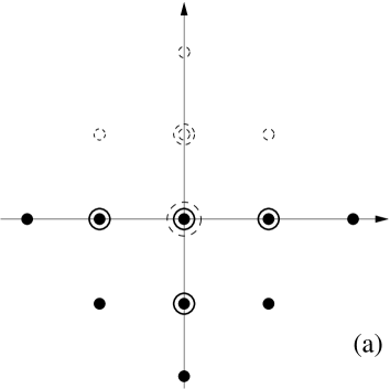
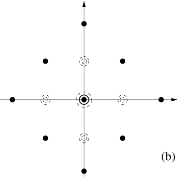
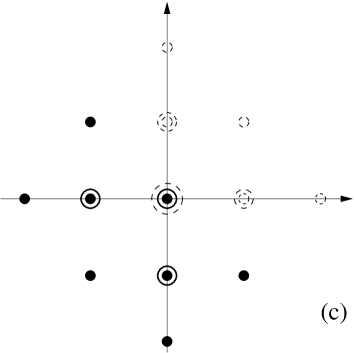
Figure 3: Root vectors of several Lie subalgebras of $\mathfrak{osp}(2|4)$, arranged in the same way as in figure 2. The full dots and circles give the generators in the respective subalgebra whereas the open dots and broken circles merely stand for the remaining generators of $\mathfrak{osp}(2|4)$. Note that in each case only two generators of the Cartan subalgebra $\mathfrak{h}$ are retained. The subalgebras are (a) $\tilde{\mathfrak{s}}^{(2)}$, (b) $(\mathfrak{conf}_{3})_{\mathbb{C}}$ and (c) $\mathfrak{se}(3|2)$.

We first need some definitions (see [11, 18, 34] for details).

Definition 2. A commutative associative algebra $\cal A$ is a Poisson algebra if there exists a Lie bracket $\{\ ,\ \}~{}:~{}{\cal A}\times{\cal A}\to{\cal A}$ (called Poisson bracket) which is compatible with the associative product $f,g\mapsto fg$, that is to say, such that the so-called Leibniz identity holds true

$$\{fg,h\}=f\{g,h\}+g\{f,h\},\quad\forall f,g,h\in{\cal A}.$$ (3.36)

This definition is naturally superizable and leads to the notion of a super-Poisson algebra. Standard examples are Poisson or super-Poisson algebras of smooth functions on supermanifolds.

In this and the following subparagraphs, we shall consider a Poisson algebra, denoted ${\cal P}^{(2m|N)}$, of functions on the $(2m|N)$-supertorus, where $m=1,2$ and $N=0,1,2$. As an associative algebra, it may be written as the tensor product

$${\cal P}^{(2m|N)}={\cal P}^{(2m|0)}\otimes\Lambda(\mathbb{R}^{N})$$ (3.37)

where $\Lambda(\mathbb{R}^{N})$ is the Grassmann algebra in the anticommuting variables $\theta^{1},\ldots,\theta^{N}$, and ${\cal P}^{(2m|0)}$ is the associative algebra generated by the functions $(q_{i},q_{i}^{-1},p_{i},p_{i}^{-1})$, $i=1,\ldots,m$, corresponding to finite Fourier series. (Note that the Poisson algebra of smooth functions on the $(2|N)$-supertorus is a kind of completion of ${\cal P}^{(2|N)}$.)

Definition 3. We denote by $\delta$ the graduation on ${\cal P}^{(2m|N)}$ defined by setting $\delta(f)=k$, with $k=0,1,\ldots,N$, for the monomials $f(q,p,\theta)=f_{0}(q,p)\theta^{i_{1}}\ldots\theta^{i_{k}}$.

The Poisson bracket is defined to be

$$\{f,g\}=\sum_{i=1}^{m}\frac{\partial f}{\partial q_{i}}\frac{\partial g}{\partial p_{i}}-\frac{\partial f}{\partial p_{i}}\frac{\partial g}{\partial q_{i}}-(-1)^{\delta(f)}\sum_{i,j=1}^{N}\eta^{i\,j}\frac{\partial f}{\partial{\theta^{i}}}\frac{\partial g}{\partial{\theta^{j}}}\ \ ,$$ (3.38)

where $\eta^{ij}$ is a non-degenerate symmetric two-tensor. Equivalently (by the Leibniz identity), it may be defined through the relations

$$\{q_{i},p_{j}\}=\delta_{i,j},\ \{q_{i},\theta^{j}\}=0,\ \{p_{i},\theta^{j}\}=0,\ \{\theta^{i},\theta^{j}\}=\eta^{ij}.$$ (3.39)

We warn the reader who is not familiar with Poisson structures in a supersymmetric setting against the familiar idea that the Poisson bracket of two functions should be obtained in a more or less straightforward way from their products. One has for instance in the case $N=1$

$$(\theta^{1})^{2}=0,\quad\{\theta^{1},\theta^{1}\}=\eta^{11}\not=0$$

which might look a little confusing at first.

It is a well-known fact (see [19] for instance) that the Schrödinger Lie algebra ${\mathfrak{sch}}_{1}$ generated by $X_{\pm 1,0},Y_{\pm{1\over 2}},M_{0}$ is isomorphic to the Lie algebra of polynomials in $(q,p)=(q_{1},p_{1})$ with degree $\leq 2$: an explicit isomorphism is given by

$$X_{-1}\to{1\over 2}q^{2}\;\;,\;\;X_{0}\to-{1\over 2}qp\;\;,\;\;X_{1}\to{1\over 2}p^{2}\;\;,\;\;Y_{-{1\over 2}}\to q\;\;,\;\;Y_{{1\over 2}}\to-p\;\;,\;\;M_{0}\to 1.$$ (3.40)

In particular, the Lie subalgebra $\langle X_{-1},X_{0},X_{1}\rangle$ of quadratic polynomials in ${\cal P}^{(2|0)}$ is isomorphic to the Lie algebra ${\mathfrak{sp}}(2,\mathbb{R})$ of linear infinitesimal canonical transformations of $\mathbb{R}^{2}$, which is a mere reformulation of the canonical isomorphism ${\mathfrak{sl}}(2,\mathbb{R})\cong{\mathfrak{sp}}(2,\mathbb{R})$ (see subsection 3.6 for an extension of this result).

We now give a natural extension of this isomorphism to a supersymmetric setting. In what follows we take $m=1,N=2$ and $\{\theta^{1},\theta^{1}\}=\{\theta^{2},\theta^{2}\}=0,\{\theta^{1},\theta^{2}\}=2.$

Definition 4 We denote by ${\cal P}^{(2|2)}_{\leq 2}\subset{\cal P}^{(2|2)}$ the Lie algebra of superfunctions that are polynomials in $(p,q,\theta^{1},\theta^{2})$ of degree $\leq 2$.

Proposition 3.4. One has an isomorphism from $\tilde{{\mathfrak{s}}}^{(2)}$ to the Lie algebra ${\cal P}^{(2|2)}_{\leq 2}$ given explicitly as

$$X_{-1}\to{1\over 2}q^{2}\;\;,\;\;X_{0}\to-{1\over 2}qp\;\;,\;\;X_{1}\to{1\over 2}p^{2}\;\;,\;\;Y_{-{1\over 2}}\to q\;\;,\;\;Y_{{1\over 2}}\to-p\;\;,\;\;M_{0}\to 1$$

$$N_{0}\to-{1\over 2}\theta^{1}\theta^{2}$$

$$\bar{Y}_{0}^{1}\to-\theta^{1}\;\;,\;\;\quad\bar{Y}_{0}^{2}\to\theta^{2}$$ (3.41)

$$G_{-{1\over 2}}^{1}\to-{1\over 2}q\theta^{1}\;\;,\;\;G_{-{1\over 2}}^{2}\to{1\over 2}q\theta^{2}$$

$$G_{{1\over 2}}^{1}\to{1\over 2}p\theta^{1}\;\;,\;\;G_{{1\over 2}}^{2}\to-{1\over 2}p\theta^{2}.$$

Remark : An equivalent statement of this result and its extension to higher spatial dimensions was given in [13], eq. (4.10). This Lie isomorphism allows a rapid computation of Lie brackets in $\tilde{{\mathfrak{s}}}^{(2)}$.

Proof. The subalgebra of ${\cal P}_{\leq 2}^{(2|2)}$ made up of the monomials of degree $0$ in $p$ decomposes as a four-dimensional commutative algebra $\langle q^{2},q,1,\theta^{1}\theta^{2}\rangle$ (for the even part), plus four odd generators $\theta^{i},q\theta^{i}$, $i=1,2$. One may easily check the identification with the 3 even translations and the ‘super-Euler operator’ $N_{0}$, plus the 4 odd translations of ${\mathfrak{se}}(3|2)$, see figure 2.

Then the two allowed rotations, $X_{0}$ and $Y_{{1\over 2}}$, form together with the translations a nine-dimensional algebra that is also easily checked to be isomorphic to its image in ${\cal P}^{(2|2)}_{\leq 2}$.

Finally, one sees immediately that the quadratic expressions (appearing just before Proposition 3.2 and inside its proof) that give $X_{1},G_{{1\over 2}}^{1,2}$ in terms of $Y,\bar{Y}$ also hold in the associative algebra ${\cal P}^{(2|2)}_{\leq 2}$ with the suggested identification (actually, this is also true for the generators $N_{0},X_{-1},X_{0},G_{-{1\over 2}}^{1,2}$, so one may still reduce the number of verifications.) $\Box$

Let us finish this paragraph by coming back to the original $N=2$ supersymmetry algebra (see subsection 3.1). Suppose we want to consider only left-invariant odd translations $D_{\theta^{1}}=-G_{-{1\over 2}}^{1}-G_{-{1\over 2}}^{2}$ and $D_{\theta^{2}}=-\bar{Y}_{0}^{1}-\bar{Y}_{0}^{2}$. It is then natural to consider the vector space

$$\tilde{{\mathfrak{s}}}^{(1)}:=\langle X_{-1},X_{0},X_{1},Y_{-{1\over 2}},Y_{{1\over 2}},M_{0},G_{-{1\over 2}}^{1}+G_{-{1\over 2}}^{2},G_{{1\over 2}}^{1}+G_{{1\over 2}}^{2},\bar{Y}_{0}^{1}+\bar{Y}_{0}^{2}\rangle$$ (3.42)

and to ask whether this is a Lie subalgebra of $\tilde{{\mathfrak{s}}}^{(2)}$. The answer is yes and this is best proved by using the Poisson algebra formulation. Since restricting to this subalgebra amounts to considering functions that depend only on $p,q$ and $\tilde{\theta}:=(\theta^{1}-\theta^{2})/(2{\rm i})$, with $(\tilde{\theta})^{2}=0$ and $\{\tilde{\theta},\tilde{\theta}\}=1$, $\tilde{{\mathfrak{s}}}^{(1)}$ can be seen as the Lie algebra of polynomials of degree $\leq 2$ in ${\cal P}^{(2|1)}$: it sits inside ${\cal P}^{(2|1)}$ just in the same way as $\tilde{{\mathfrak{s}}}^{(2)}$ sits inside ${\cal P}^{(2|2)}$. Of course, the conjugate algebra obtained by taking the same linear combinations, but with a minus sign instead (that is, generated by $X_{\pm 1,0},Y_{\pm{1\over 2}},G_{{1\over 2}}^{1}-G_{{1\over 2}}^{2}$ and the right-invariant odd translations $\bar{D}_{\theta^{1}}=G_{-{1\over 2}}^{2}-G_{-{1\over 2}}^{1}$ and $\bar{D}_{\theta^{2}}=\bar{Y}_{0}^{2}-\bar{Y}_{0}^{1}$) is isomorphic to $\tilde{{\mathfrak{s}}}^{(1)}$. The commutation relations of $\tilde{{\mathfrak{s}}}^{(1)}$ are again illustrated in figure 3a, where the four double circles of a pair of generators should be replaced by a single generator. We shall consider this algebra once again in section 5.

3.6 Second correspondence with Poisson structures: the case of $\mathfrak{osp}(2|4)$, or the $(3|2)$-supersymmetric model

We shall prove in this subsection Proposition 3.3 by giving an embedding of the vector space ${\mathfrak{s}}^{(2)}$ into a Poisson algebra, from which the fact that ${\mathfrak{s}}^{(2)}$ closes as a Lie algebra becomes self-evident.

Let us first recall the definition of the orthosymplectic superalgebras.

Definition 5. Let $n,m=1,2,\ldots$ The Lie superalgebra ${\mathfrak{osp}}(n|2m)$ is the set of linear vector fields in the coordinates $x^{1},\ldots,x^{2m},\theta^{1},\ldots,\theta^{n}$ preserving the 2-form $\sum_{i=1}^{m}{\rm d}x^{i}\wedge{\rm d}x^{m+i}+\sum_{j=1}^{n}({\rm d}\theta^{i})^{2}.$

In the following proposition, we recall the folklore result which states that the Lie superalgebra ${\mathfrak{osp}}(2|2m)$ may be embedded into a super-Poisson algebra of functions on the $(2m|2)$-supertorus, and detail the root structure in this very convenient embedding.

Definition 6. We denote by ${\cal P}^{(2m|2)}_{(2)}$ the Lie subalgebra of quadratic polynomials in the super-Poisson algebra ${\cal P}^{(2m|2)}$ on the $(2m|2)$-supertorus.

Proposition 3.5. Equip the super-Poisson algebra ${\cal P}^{(2m|2)}$ with the super-Poisson bracket $\{q_{i},p_{j}\}=\delta_{i,j},\{\theta^{1},\theta^{2}\}=2,$ and consider its Lie subalgebra ${\cal P}^{(2m|2)}_{(2)}\subset{\cal P}^{(2m|2)}$. Then

1. The Lie algebra ${\cal P}^{(2m|2)}_{(2)}$ is isomorphic to ${\mathfrak{osp}}(2|2m)$.

2. Using this isomorphism, a Cartan subalgebra of ${\mathfrak{osp}}(2|2m)$ is given by $p_{i}q_{i}$ ($i=1,\ldots,2m$) and $\theta^{1}\theta^{2}$. Let $(f_{1},\ldots,f_{2m},\alpha)$ be the dual basis. Then the root-space decomposition is given by

   $${\mathfrak{osp}}(2|2m)={\mathfrak{osp}}(2|2m)_{0} \oplus {\mathfrak{osp}}(2|2m)_{f_{i}-f_{j}}\oplus{\mathfrak{osp}}(2|2m)_{\pm(f_{i}+f_{j})}$$

   $$\oplus {\mathfrak{osp}}(2|2m)_{\pm 2f_{i}}\oplus{\mathfrak{osp}}(2|2m)_{\pm f_{i}+2\alpha}\oplus{\mathfrak{osp}}(2|2m)_{\pm f_{i}-2\alpha}\;(i\not=j)$$

   Except ${\mathfrak{osp}}(2|2m)_{0}$ which is equal to the Cartan subalgebra, all other root-spaces are one-dimensional, and

   $${\mathfrak{osp}}(2|2m)_{f_{i}-f_{j}}\>=\>\langle p_{i}q_{j}\rangle\;\;,\;\;{\mathfrak{osp}}(2|2m)_{f_{i}+f_{j}} = \langle p_{i}p_{j}\rangle\;\;,\;\;{\mathfrak{osp}}(2|2m)_{-(f_{i}+f_{j})}\>=\>\langle q_{i}q_{j}\rangle$$

   $${\mathfrak{osp}}(2|2m)_{2f_{i}} = \langle p_{i}^{2}\rangle\;\;\>\;\;,\;\;{\mathfrak{osp}}(2|2m)_{-2f_{i}}\>=\>\langle q_{i}^{2}\rangle$$

   $${\mathfrak{osp}}(2|2m)_{f_{i}+2\alpha} = \langle p_{i}\theta^{1}\rangle\;\;,\;\;{\mathfrak{osp}}(2|2m)_{-f_{i}+2\alpha}\>=\>\langle q_{i}\theta^{1}\rangle$$

   $${\mathfrak{osp}}(2|2m)_{f_{i}-2\alpha} = \langle p_{i}\theta^{2}\rangle\;\;,\;\;{\mathfrak{osp}}(2|2m)_{-f_{i}-2\alpha}\>=\>\langle q_{i}\theta^{2}\rangle.$$ (3.44)

Proof. Straightforward. $\Box$

The root structure is illustrated in figure 2 in the case $m=2$. We may now finally state the last ingredient for proving Proposition 3.3.

Proposition 3.6.

1. The linear application $\tilde{{\mathfrak{s}}}^{(2)}\to{\mathfrak{osp}}(2|4)$ defined on generators by

   $$X_{-1} \to {1\over 2}q_{1}^{2}\;\;,\;\;X_{0}\to-{1\over 2}q_{1}p_{1}\;\;,\;\;X_{1}\to{1\over 2}p_{1}^{2}\;\;,\;\;Y_{-{1\over 2}}\to q_{1}q_{2}\;\;,\;\;Y_{{1\over 2}}\to-p_{1}q_{2}\;\;,\;\;M_{0}\to q_{2}^{2}$$

   $$N_{0} \to {1\over 2}\theta^{1}\theta^{2}$$

   $$\bar{Y}_{0}^{1} \to -q_{2}\theta^{1}\;\;,\;\;\bar{Y}_{0}^{2}\to q_{2}\theta^{2}$$ (3.45)

   $$G_{-{1\over 2}}^{1} \to -{1\over 2}q_{1}\theta^{1}\;\;,\;\;G_{{1\over 2}}^{1}\to{1\over 2}p_{1}\theta^{1}\;\;,\;\;G_{-{1\over 2}}^{2}\to{1\over 2}q_{1}\theta^{2}\;\;,\;\;G_{{1\over 2}}^{2}\to-{1\over 2}p_{1}\theta^{2},$$

   where $i=1,2$, is a Lie algebra morphism and gives an embedding of $\tilde{{\mathfrak{s}}}^{(2)}$ into ${\mathfrak{osp}}(2|4)$.

2. This application can be extended into a Lie algebra isomorphism from ${\mathfrak{s}}^{(2)}$ onto ${\mathfrak{osp}}(2|4)$ by putting

   $$D\to-{1\over 2}(q_{1}p_{1}+q_{2}p_{2})\;\;,\;\;V_{+}\to p_{1}p_{2}\;\;,\;\;W\to\frac{1}{4}p_{2}^{2}\;\;,\;\;V_{-}\to-\frac{1}{4}q_{1}p_{2}\;\;,\;\;\bar{Z}_{0}^{1}\to\frac{1}{8}p_{2}\theta^{1}\;\;,\;\;\bar{Z}_{0}^{2}\to-\frac{1}{8}p_{2}\theta^{2}.$$ (3.46)

Proof. The first part is an immediate consequence of proposition 3.4. One merely needs to replace $q,p$ by $q_{1},p_{1}$ and then make all generators quadratic in the variables $p_{1},p_{2},q_{1},q_{2},\theta^{1},\theta^{2}$ by multiplying with the appropriate power of $q_{2}$.

We now turn to the second part. The root diagram of ${\mathfrak{osp}}(2|4)$ in figure 2 helps to understand. First $\langle\bar{Z}_{0}^{1,2},G_{{1\over 2}}^{1,2};W,V_{+},X_{1}\rangle$ form a Lie algebra of dimension 7 that is isomorphic to $\langle p_{2}\theta^{1,2},p_{1}\theta^{1,2},p_{2}^{2},p_{1}p_{2},p_{1}^{2}\rangle$: in particular, the even part $\langle W,V_{+},X_{1}\rangle$ is commutative and commutes with the 4 other generators; brackets of the odd generators $\bar{Z}_{0}^{1,2},G_{{1\over 2}}^{1,2}$ yield the whole vector space $\langle W,V_{+},X_{1}\rangle$. Note that part of these computations (commutators of $X_{1},G^{1,2}_{{1\over 2}}$) come from the preceding subsection, the rest must be checked explicitly. So all there remains to be done is to check for the adjoint action of $\bar{Z}^{0}_{1,2},G_{{1\over 2}}^{1,2}$ on ${\mathfrak{se}}(3|2)$. We already computed the action of $G_{{1\over 2}}^{1,2}$ on (even or odd) translations; in particular, $G_{{1\over 2}}^{1,2}$ preserves this subspace. On the other hand, commutators of $G_{{1\over 2}}^{1,2}$ with rotations $V_{-},X_{0},N_{0},Y_{{1\over 2}}$ yield linear combinations of $\bar{Z}_{0}^{1,2}$ and $G_{{1\over 2}}^{1,2}$: by definition,

$$[G_{{1\over 2}}^{1,2},V_{-}]=\bar{Z}_{0}^{1,2}$$

while other commutators $[G_{{1\over 2}}^{1,2},X_{0}]={1\over 2}G_{{1\over 2}}^{1,2},[G_{{1\over 2}}^{1},N_{0}]=-G_{{1\over 2}}^{1},[G_{{1\over 2}}^{2},N_{0}]=G_{{1\over 2}}^{2},[G_{{1\over 2}}^{1,2},Y_{{1\over 2}}]=0$ are already known. Now the symmetry $t\leftrightarrow\zeta,\theta^{1}\leftrightarrow\theta^{2}$ preserves ${\mathfrak{se}}(3|2)$ and sends $G_{{1\over 2}}^{1,2}$ into $2\bar{Z}_{0}^{1,2}$, and corresponds to the symmetry $p\leftrightarrow q$ on ${\mathfrak{osp}}(2|4)\cong{\cal P}^{(4|2)}_{(2)}$, so the action of $\bar{Z}_{0}^{1,2}$ on the rotation-translation symmetry algebra is the right one. Finally, since $W,V_{+}$ and $X_{1}$ are given by commutators of $G_{{1\over 2}}^{1,2}$ and $\bar{Z}_{0}^{2}$, and the commutators of $D$ with the other generators are easily checked to be correct, we are done. $\Box$

In section 5 we shall consider two-point functions that are covariant under the vector space $\tilde{{\mathfrak{s}}}^{(2)}_{1}=\langle X_{-1},G_{-{1\over 2}}^{1,2},X_{0},N_{0},G_{{1\over 2}}^{1,2},X_{1}\rangle\subset\tilde{{\mathfrak{s}}}^{(2)}$ (actually $\tilde{{\mathfrak{s}}}_{1}^{(2)}\subset\tilde{{\mathfrak{s}}}^{(2)}$ is made of symmetries of the super-Schrödinger model). On the root diagram figure 2, the generators of $\tilde{{\mathfrak{s}}}^{(2)}_{1}$ are all on the $f_{1}$-axis, hence (as one sees easily) $\tilde{{\mathfrak{s}}}^{(2)}_{1}$ is a Lie algebra. The following proposition gives several equivalent characterizations of $\tilde{{\mathfrak{s}}}^{(2)}_{1}$. We omit the easy proof.

Proposition 3.7

1. The embedding $\tilde{{\mathfrak{s}}}^{(2)}\subset{\cal P}^{(2|2)}_{\leq 2}$ of eq. (3.41) in Proposition 3.4 maps $\tilde{{\mathfrak{s}}}_{1}^{(2)}$ onto ${\cal P}_{(2)}^{(2|2)}$. Hence, by Proposition 3.5, $\tilde{{\mathfrak{s}}}^{(2)}_{1}\cong{\mathfrak{osp}}(2|2).$

2. The Poisson bracket on ${\cal P}_{\leq 2}^{(2|2)}$ (see Proposition 3.4) is of degree -1 with respect to the graduation $\widetilde{{\rm deg\,}}$ of ${\cal P}^{(2|2)}$ defined by $\widetilde{{\rm deg\,}}(q)=\widetilde{{\rm deg\,}}(p)=\widetilde{{\rm deg\,}}(\theta^{i})={1\over 2}$: in other words, $\widetilde{{\rm deg\,}}\ \{f,g\}=\widetilde{{\rm deg\,}}f+\widetilde{{\rm deg\,}}g-1$ for $f,g\in{\cal P}^{(2|2)}$. Hence the set $\{X\in{\cal P}^{(2|2)}\ |\ \widetilde{{\rm deg\,}}(X)=1\}\cong\tilde{{\mathfrak{s}}}_{1}^{(2)}$ is a Lie subalgebra of ${\cal P}^{(2|2)}$.

3. The Poisson bracket on ${\cal P}_{(2)}^{(4|2)}$ (see Proposition 3.5) is of degree -1 with respect to the graduation ${\rm deg\,}$ of ${\cal P}^{(4|2)}$ defined by ${\rm deg\,}(q_{1})={\rm deg\,}(p_{1})={\rm deg\,}(\theta^{1})={\rm deg\,}(\theta^{2})={1\over 2},{\rm deg\,}(p_{2})=1,{\rm deg\,}(q_{2})=0$. Hence the set $\{X\in{\cal P}_{(2)}^{(4|2)}\ |\ {\rm deg\,}(X)=1\}\cong\tilde{{\mathfrak{s}}}_{1}^{(2)}\oplus\mathbb{R}D$ is a Lie subalgebra of ${\cal P}^{(4|2)}$.

Note that points 1 and 2 use the first correspondence (see eq. (3.41) in Proposition 3.4) while point 3 uses the second correspondence (see eqs. (3.45,3.46) in Proposition 3.6).

4 Extended Schrödinger and super-Schrödinger transformations

We shall be looking in this section for infinite-dimensional extensions of various Lie algebras of Schrödinger type (${\mathfrak{sch}}_{1},\tilde{{\mathfrak{s}}}^{(1)},\tilde{{\mathfrak{s}}}^{(2)},\tilde{{\mathfrak{s}}}^{(2)}_{1}\cong{\mathfrak{osp}}(2|2)$) that we introduced until now, hoping that these infinite-dimensional Lie algebras or super-algebras might play for anisotropic systems a role analogous to that of the Virasoro algebra in conformal field theory [5]. Note that the Lie superalgebra ${\mathfrak{s}}^{(2)}\cong{\mathfrak{osp}}(2|4)$ was purposely not included in this list, nor could ${\mathfrak{conf}}_{3}$ be included: it seems that there is a ‘no-go theorem’ preventing this kind of embedding of Schrödinger-type algebras into infinite-dimensional Virasoro-like algebras to extend to an embedding of the whole conformal-type Lie algebra (see [44]).

In the preceding section, we saw that all Schrödinger or super-Schrödinger or conformal or ‘super-conformal’ Lie symmetry algebras could be embedded in different ways into some Poisson algebra or super-algebra ${\cal P}^{(n|N)}$.

We shall extend the Schrödinger-type Lie algebras by embedding them in a totally different way into some of the following ‘twisted’ Poisson algebras, where, roughly speaking, one is allowed to consider the square-root of the coordinate $p$.

Definition 7. The twisted Poisson algebra $\widetilde{\cal P}^{(2|N)}$ is the associative algebra of super-functions

$$f(p,q;\theta):=f(p,q;\theta^{1},\ldots,\theta^{N})=\sum_{i\in{1\over 2}\mathbb{Z}}\sum_{j\in\mathbb{Z}}\sum_{k=1}^{N}\sum_{i_{1}<\ldots<i_{k}}c_{i,j,i_{1},\ldots,i_{k}}p^{i}q^{j}\theta^{i_{1}}\ldots\theta^{i_{k}}$$ (4.1)

with usual multiplication and Poisson bracket defined by

$$\{f,g\}:={\partial f\over\partial q}{\partial g\over\partial p}-{\partial f\over\partial p}{\partial g\over\partial q}-(-1)^{\delta(f)}\sum_{i=1}^{N}\partial_{\theta^{i}}f\partial_{\theta^{i}}g$$ (4.2)

with the graduation $\delta:\widetilde{\cal P}^{(2|N)}\to\mathbb{N}$ defined as a natural extension of Definition 3 (see subsection 3.5) on the monomials by

$$\delta(f(p,q)\theta^{i_{1}}\ldots\theta^{i_{k}}):=k.$$ (4.3)

The Poisson bracket may be defined more loosely by setting $\{q,p\}=1,\ \{\theta^{i},\theta^{j}\}=\delta^{i,j}$ and applying the Leibniz identity.

Definition 8. We denote by ${\rm gra\,}:\widetilde{\cal P}^{(2|N)}\to\{0,{1\over 2},1,\ldots\}$ the graduation (called grade) on the associative algebra $\widetilde{\cal P}^{(2|N)}$ defined by

$${\rm gra\,}(q^{n}p^{m}\theta^{i_{1}}\ldots\theta^{i_{k}}):=m+k/2$$ (4.4)

on monomials.

This graduation may be defined more simply by setting ${\rm gra\,}(q)=0,\ {\rm gra\,}(p)=1,\ {\rm gra\,}(\theta^{i})={1\over 2}$. Note that it is closely related but clearly different from the graduations ${\rm deg\,},\ \widetilde{{\rm deg\,}}$ defined on untwisted Poisson algebras in Proposition 3.7.

Definition 9. We denote by $\widetilde{\cal P}^{(2|N)}_{\leq\kappa},\ \ \kappa\in{1\over 2}\mathbb{Z}$ (resp. $\widetilde{\cal P}^{(2|N)}_{(\kappa)}$) the vector subspace of $\widetilde{\cal P}^{(2|N)}$ consisting of all elements of grade $\leq\kappa$ (resp. of grade equal to $\kappa$).

Since the Poisson bracket is of grade -1 (as was the case for ${\rm deg\,}$ and $\widetilde{{\rm deg\,}}$) it is clear that $\widetilde{\cal P}^{(2|N)}_{\leq\kappa}$ (resp. $\widetilde{\cal P}^{(2|N)}_{(\kappa)}$) is a Lie algebra if and only if $\kappa\leq 1$ (resp. $\kappa=1$).

It is also easy to check, by the same considerations, that $\widetilde{\cal P}_{\leq\kappa}^{(2|N)}$ $(\kappa\leq{1\over 2})$ is a (proper) Lie ideal of $\widetilde{\cal P}_{\leq 1}^{(2|N)}$, so one may consider the resulting quotient algebra. In the following, we shall restrict to the case $\kappa=-{1\over 2}$ and define the Schrödinger-Neveu-Schwarz algebra ${\mathfrak{sns}}^{(N)}$ by

$${\mathfrak{sns}}^{(N)}:=\widetilde{\cal P}_{\leq 1}^{(2|N)}/\widetilde{\cal P}_{\leq-1/2}^{(2|N)}$$ (4.5)

The choice for the name is by reference to the case $N=1$ (see below).

4.1 Elementary examples

Table 2: Conformal dimensions ${\rm cdim\,}$ of the generators of the three supersymmetric extensions ${\mathfrak{sv}}$, $\mathfrak{sns}^{(1)}$ and $\mathfrak{sns}^{(2)}$ of the one-dimensional Schrödinger algebra $\mathfrak{sch}_{1}$.

	${\rm cdim\,}$	pair	impair
${\mathfrak{sv}}$	2	$X$
	$3/2$	$Y$
	1	$M$
$\mathfrak{sns}^{(1)}$	2	$X$
	$3/2$	$Y$	$G$
	1	$M$	$\bar{Y}$
	$1/2$		$\bar{M}$
$\mathfrak{sns}^{(2)}$	2	$X$
	$3/2$	$Y$	$G^{1}$, $G^{2}$
	1	$M$, $N$	$\bar{Y}^{1}$, $\bar{Y}^{2}$
	$1/2$	$P$	$\bar{M}^{1}$, $\bar{M}^{2}$
	0	$Q$

Table 3: Grades ${\rm gra\,}$ of the generators of the three supersymmetric extensions ${\mathfrak{sv}}$, $\mathfrak{sns}^{(1)}$ and $\mathfrak{sns}^{(2)}$ of the one-dimensional Schrödinger algebra $\mathfrak{sch}_{1}$.

	${\rm gra\,}$	pair	impair
${\mathfrak{sv}}$	1	$X$
	$1/2$	$Y$
	0	$M$
$\mathfrak{sns}^{(1)}$	1	$X$	$G$
	$1/2$	$Y$	$\bar{Y}$
	0	$M$	$\bar{M}$
$\mathfrak{sns}^{(2)}$	1	$X$, $N$	$G^{1}$, $G^{2}$
	$1/2$	$Y$, $P$	$\bar{Y}^{1}$, $\bar{Y}^{2}$
	0	$M$, $Q$	$\bar{M}^{1}$, $\bar{M}^{2}$

Let us study in this subsection the simplest examples $N=0,1.$

• $N=0$.

  The Lie algebra ${\mathfrak{sns}}^{(0)}$ is generated by (images in the quotient $\widetilde{\cal P}_{\leq 1}^{(2|0)}/\widetilde{\cal P}_{\leq-1/2}^{(2|0)}$ ) of the fields $X,Y,M$ defined by

  $$X_{\phi}=\phi(q)p\;\;,\;\;Y_{\phi}=\phi(q)p^{{1\over 2}}\;\;,\;\;M_{\phi}=\phi(q).$$ (4.6)

  By computing the commutators in the quotient, we see that ${\mathfrak{sns}}^{(0)}={\mathfrak{sv}}$ is the Schrödinger-Virasoro algebra eq. (1.2), with mode expansion $X_{n}=q^{n+1}p$, $Y_{m}=q^{m+{1\over 2}}p^{{1\over 2}}$, $M_{n}=q^{n}$ (where $n\in\mathbb{Z}$, $m\in\mathbb{Z}+{1\over 2}$). Each of these three fields $A=X,Y$ or $M$ has a mode expansion of the form $A_{n}=q^{n+\varepsilon}p^{\varepsilon}$. We may rewrite this as $A_{\lambda-\varepsilon}=q^{\lambda}p^{\varepsilon}$ with $\lambda\in\mathbb{Z}+\varepsilon$ and see that the shift $\varepsilon$ in the indices of the generators (with respect to the power of $q$) is equal to the opposite of the power of $p$. This will also hold true for any value of $N$.

  It is important to understand that successive ‘commutators’ $\{Y_{\phi},M_{\psi}\},\{Y_{\phi_{1}},\{Y_{\phi_{2}},M_{\psi}\}\},\ldots$ in $\widetilde{\cal P}_{\leq 1}^{(2|0)}$ are generally non-zero and yield ultimately the whole algebra $\widetilde{\cal P}_{\leq-{1\over 2}}^{(2|0)}$. This is due to the fact that derivatives of $p^{{1\over 2}}$ give $p$ to power $-{1\over 2},-{3\over 2},\ldots$, unlike derivatives of integer positive powers of $p$, which cancel after a finite time and give only polynomials in $p$.

  The algebraic structure of ${\mathfrak{sv}}$ is as follows, see (1.2). It is the semi-direct product ${\mathfrak{sv}}={\mathfrak{vir}}\ltimes{\mathfrak{h}}^{(0)}:=\langle X_{n}\rangle_{n\in\mathbb{Z}}\ltimes\langle Y_{m},M_{p}\rangle_{m\in{1\over 2}+\mathbb{Z},p\in\mathbb{Z}}$ of a centreless Virasoro algebra and of a two-step nilpotent (that is to say, whose brackets are central) Lie algebra generated by the $Y_{m}$ and $M_{n}$, extending the Heisenberg algebra ${\mathfrak{h}}_{1}$. The inclusion ${\mathfrak{sch}}_{1}\cong{\mathfrak{sl}}(2,\mathbb{R})\ltimes{\mathfrak{h}}_{1}\subset{\mathfrak{vir}}\ltimes{\mathfrak{h}}^{(0)}$ (see the introduction) respects the semi-direct product structure. If one considers the generators $X_{n}$, $Y_{m}$ and $M_{n}$ as the components of associated conserved currents $X,Y$ and $M$, then $X$ is a Virasoro field, while $Y,M$ are primary with respect to $X$, with conformal dimensions $\frac{3}{2}$, respectively $1$.

  Note also that the conformal dimension of the $\varepsilon$-shifted field $A^{\varepsilon}$ $(A^{\varepsilon}=X,Y,M)$ with mode expansion $A^{\varepsilon}_{n}=q^{n+\varepsilon}p^{\varepsilon}$ $(\varepsilon=0,{1\over 2},1)$ is equal to $1+\varepsilon$. This fact is also a general one (see subsection 4.2 below).

  For later use, we collect in tables 2 and 3 the conformal dimensions and grades of the generators of ${\mathfrak{sns}}^{(N)}$, with $N=0,1,2$.

• $N=1$.

  The Lie algebra ${\mathfrak{sns}}^{(1)}$ is generated by (images in the quotient) of the even functions $X_{\phi}=\phi(q)p,Y_{\phi}=\phi(q)p^{{1\over 2}},M_{\phi}=\phi(q)$, and of the odd functions $G_{\phi}=\phi(q)\theta^{1}p^{{1\over 2}},\bar{Y}_{\phi}=\phi(q)\theta^{1},\bar{M}_{\phi}=\phi(q)\theta^{1}p^{-{1\over 2}}$. We use the same notation as in the case $N=0$ for the mode expansions $X_{n}=q^{n+1}p,M_{n}=q^{n},\bar{Y}_{n}=q^{n}\theta^{1}$ $(n\in\mathbb{Z})$, $Y_{m}=q^{m+{1\over 2}}p^{{1\over 2}},G_{m}=q^{m+{1\over 2}}p^{{1\over 2}}\theta^{1},\bar{M}_{m}=q^{m-{1\over 2}}p^{-{1\over 2}}\theta^{1}$ ($m\in{1\over 2}+\mathbb{Z}$), with the same shift in the indices, equal to the opposite of the power in $p$.

  We have a semi-direct product structure $\mathfrak{sns}^{(1)}={\mathfrak{ns}}\ltimes{\mathfrak{h}}^{(1)}$, where

  $${\mathfrak{ns}}:=\langle X,G\rangle$$ (4.7)

  is isomorphic to the Neveu-Schwarz algebra [38] with a vanishing central charge, and

  $${\mathfrak{h}}^{(1)}=\langle(Y,\bar{Y}),(M,\bar{M})\rangle.$$ (4.8)

  The commutators of $G$ with these fields read in mode expansion (where we identify the Poisson bracket with an (anti)commutator)

  $${}[G_{n},Y_{m}] = {1\over 2}(n-m)\bar{Y}_{n+m}\;\;,\;\;{}[G_{n},\bar{Y}_{m}]=Y_{n+m}$$

  $${}[G_{n},M_{m}] = -{1\over 2}m\bar{M}_{n+m}\;\;,\;\;{}[G_{n},\bar{M}_{m}]=M_{n+m}.$$ (4.9)

  The Lie algebra ${\mathfrak{h}}^{(1)}$ is two-step nilpotent, which is obvious from the definition of the quotient: the only non-trivial brackets are between elements $Y_{\phi}$ and $\bar{Y}_{\phi}$ of grade ${1\over 2}$ and give elements $M_{\phi}$ or $\bar{M}_{\phi}$ of grade 0. Explicitly, we have:

  $${}[Y_{n},Y_{m}]={1\over 2}(n-m)M_{n+m}\;\;,\;\;{}[\bar{Y}_{n},\bar{Y}_{m}]=M_{n+m}\;\;,\;\;{}[Y_{n},\bar{Y}_{m}]=-{1\over 2}m\bar{M}_{n+m}.$$ (4.10)

  The fields $(X,G),$ $(Y,\bar{Y})$ and $(M,\bar{M})$ can be seen as supersymmetric doublets of conformal fields with conformal dimensions $(2,{3\over 2}),\ ({3\over 2},1),\ (1,{1\over 2})$, see also table 2. Once again, the conformal dimension of any of those fields is equal to the power of $p$ plus one. The grades of the fields are given by, see table 3

  $${\rm gra\,}(X_{\phi})={\rm gra\,}(G_{\phi})=1\;\;,\;\;{\rm gra\,}(Y_{\phi})={\rm gra\,}(\bar{Y}_{\phi})={1\over 2}\;\;,\;\;{\rm gra\,}(M_{\phi})={\rm gra\,}(\bar{M}_{\phi})=0.$$ (4.11)

4.2 General case

We shall actually mainly be interested in the case $N=2$, but the algebra ${\mathfrak{sns}}^{(2)}$ is quite large and one needs new insight to study it properly. So let us consider first the main features of the general case.

By considering the grading ${\rm gra\,}$, one sees immediately that ${\mathfrak{sns}}^{(N)}$ has a semi-direct product structure

$${\mathfrak{sns}}^{(N)}={\mathfrak{g}}^{(N)}\ltimes{\mathfrak{h}}^{(N)}$$ (4.12)

where the Lie algebra ${\mathfrak{g}}^{(N)}$ contains the elements of grade one and the nilpotent algebra ${\mathfrak{h}}^{(N)}$ contains the elements of grade ${1\over 2}$ or $0$. The algebra ${\mathfrak{g}}^{(N)}$ has been studied by Leites and Shchepochkina [34] as one of the ‘stringy’ superalgebras, namely, the superalgebra ${\mathfrak{k}}(1|N)$ of supercontact vector fields on the supercircle $S^{(1|N)}$. Let us just mention that ${\mathfrak{g}}^{(N)}$ shows up as a geometric object, namely, as the superalgebra of vector fields preserving the (kernel of the) 1-form ${\rm d}q+\sum_{i=1}^{N}\theta^{i}{\rm d}\theta^{i}.$ Recall also that a supercontact vector field $X$ can be obtained from its generating function $f=f(q,\theta^{1},\ldots,\theta^{N})$ by putting

$$X_{f}=-(1-{1\over 2}E)(f)\partial_{q}-{1\over 2}\partial_{q}fE-(-1)^{\delta(f)}\sum_{i=1}^{N}\partial_{\theta^{i}}f\partial_{\theta^{i}},$$ (4.13)

where $E:=\sum_{i=1}^{N}\theta^{i}\partial_{\theta^{i}}$ is the Euler operator for odd coordinates, and $\delta$ is the eigenvalue of $E$ for homogeneous superfunctions as defined in (4.3). Then one has

$$[X_{f},X_{g}]=X_{\{f,g\}_{{\mathfrak{k}}(1|N)}}$$ (4.14)

where $[\ ,\ ]$ is the usual Lie bracket of vector fields, and the contact bracket $\{\ ,\ \}_{{\mathfrak{k}}(1|N)}$ is given by

$$\{f,g\}_{{\mathfrak{k}}(1|N)}:=-(1-{1\over 2}E)(f)\partial_{q}g+\partial_{q}f(1-{1\over 2}E)(g)-(-1)^{\delta(f)}\sum_{i=1}^{N}\partial_{\theta^{i}}f\partial_{\theta^{i}}g.$$ (4.15)

Proposition 4.1 The Lie algebras ${\mathfrak{g}}^{(N)}$ and ${\mathfrak{k}}(1|N)$ are isomorphic.

Proof: Let $f=f(q,\theta)$ and $g=g(q,\theta)$ be two $E$-homogeneous superfunctions. Then

$$\tilde{f}(q,p,\theta)=f(q,\theta)\cdot p^{1-\delta(f)/2},\quad\tilde{g}(q,p,\theta)=g(q,\theta)\cdot p^{1-\delta(g)/2}$$ (4.16)

belong to the subalgebra of elements of grade one in $\widetilde{\cal P}^{(2|N)}$. Formula (4.2) for the Lie bracket of $\widetilde{\cal P}^{(2|N)}$ entails

$$\{\tilde{f},\tilde{g}\}(q,p,\theta)=\left[(1-{\delta(g)\over 2})(\partial_{q}f)g-(1-{\delta(f)\over 2})f(\partial_{q}g)\right]p^{1-{\delta(f)+\delta(g)\over 2}}-(-1)^{\delta(f)}\left[\sum_{i=1}^{N}\partial_{\theta^{i}}f\partial_{\theta^{i}}g\right]p^{2-{\delta(f)+\delta(g)\over 2}}$$

while formula (4.15) for the contact bracket yields

$$\widetilde{\{f,g\}}_{{\mathfrak{k}}(1|N)}(q,p,\theta) = -\left[(1-{1\over 2}\delta(f))f(\partial_{q}g)-(1-{1\over 2}\delta(g))(\partial_{q}f)g\right]p^{1-{1\over 2}(\delta(f)+\delta(g))}$$

$$-(-1)^{\delta(f)}\left[\sum_{i=1}^{N}\partial_{\theta^{i}}f\partial_{\theta^{i}}g\right]p^{1-{1\over 2}(\delta(f)+\delta(g)-2)}.$$

Hence

$$\{\tilde{f},\tilde{g}\}_{\widetilde{\cal P}^{(2|N)}}=\widetilde{\{f,g\}}_{{\mathfrak{k}}(1|N)}.$$

So the assignment $f\to\tilde{f}$ according to (4.16) defines indeed a Lie algebra isomorphism from ${\mathfrak{k}}(1|N)$ onto ${\mathfrak{g}}^{(N)}$. $\Box$

The application $f\to\tilde{f}$ just constructed may be extended in the following natural way.

Proposition 4.2 Assign to any superfunction $f(q,\theta)$ on $S^{(1|N)}$ the following superfunctions in the Poisson superalgebra $\widetilde{\cal P}^{(2|N)}$:

$$f^{(\alpha)}(q,p,\theta):=f(q,\theta)\cdot p^{\alpha-\delta(f)/2},\quad\alpha\in{1\over 2}\mathbb{Z}$$ (4.17)

so that, in particular, $f^{(1)}=\tilde{f}$ as defined in (4.16). Then $f\to f^{(\alpha)}$ defines a linear isomorphism from the algebra of superfunctions on $S^{(1|N)}$ into the vector space of superfunctions in $\widetilde{\cal P}^{(2|N)}$ with grade $\alpha$, and the Lie bracket (4.2) on the Poisson algebra may be written in terms of the superfunctions on $S^{(1|N)}$ in the following way: let $f,g$ be two $E$-homogeneous functions on $S^{(1|N)}$,

$$\{f^{(\alpha)},g^{(\beta)}\}_{\widetilde{\cal P}^{(2|N)}}=\left(-(\alpha-{1\over 2}E)(f)\partial_{q}g-\partial_{q}f(\beta-{1\over 2}E)(g)-(-1)^{\delta(f)}\sum_{i=1}^{N}\partial_{\theta^{i}}f\partial_{\theta^{i}}g\right)^{(\alpha+\beta-1)}.$$ (4.18)

Proof. Similar to the proof of proposition 4.1. $\Box$

Coming back to ${\mathfrak{sns}}^{(N)}$, we restrict to the values $\alpha=1,{1\over 2},0$. Put $f_{n}(q)=q^{n+1}$ $(n\in\mathbb{Z})$ and $g_{m}(q)=q^{m+\alpha-|I|/2}\theta^{I}$, where $I=\{i_{1}<\cdots<i_{k}\}\subset\{1,\ldots,N\}$ and $\theta^{I}:=\theta^{i_{1}}\wedge\cdots\wedge\theta^{i_{k}},$ and $m\in\mathbb{Z}-\alpha+|I|/2$. Then

$$\{f_{n}^{(1)},g_{m}^{(\alpha)}\}_{\widetilde{\cal P}^{(2|N)}} = \{q^{n+1}p,q^{m+\alpha-|I|/2}\theta^{I}p^{\alpha-|I|/2}\}_{{\cal P}^{(2|N)}}$$ (4.19)

$$= \left[-(m+\alpha-|I|/2)+(\alpha-{1\over 2}|I|)(n+1)\right]q^{n+m+\alpha-|I|/2}\theta^{I}p^{\alpha-|I|/2}$$

$$= ((\alpha-|I|/2)n-m)g_{n+m}^{(\alpha)},$$

so the $\tilde{f}_{n}=f^{(1)}_{n}$ may be considered as the components of a centreless Virasoro field $X$, while the $g_{m}^{(\alpha)}$ are the components of a primary field $Z_{\alpha}^{I}$, with conformal dimension $1+\alpha-|I|/2$, in the sense of [5].

Note also that, as in the cases $N=0,1$ studied in subsection 4.1, the conformal dimension ${\rm cdim\,}$ of each field is equal to the power of $p$ plus one, and the shift in the indices (with respect to the power of $q$) is equal to the opposite of the power of $p$.

4.3 Study of the case $N=2$.

As follows from the preceding subsection, the superalgebra ${\mathfrak{sns}}^{(2)}$ is generated by the fields $Z_{\alpha}^{I}$ where $I=\emptyset,\ \{1\},\ \{2\}$ or $\{1,2\}$ and $\alpha=0,{1\over 2}$ or $1$. Set

$$X=Z_{1}^{\emptyset}\;\;,\;\;G^{1,2}={1\over\sqrt{2}}\left(Z_{1}^{\{1\}}\pm{\rm i}Z_{1}^{\{2\}}\right)\;\;,\;\;N={\rm i}\sqrt{2}Z_{1}^{\{1,2\}}$$ (4.20)

for generators of grade one,

$$Y=\sqrt{2}Z_{{1\over 2}}^{\emptyset}\;\;,\;\;\bar{Y}^{1,2}=\pm Z_{{1\over 2}}^{\{1\}}+{\rm i}Z_{{1\over 2}}^{\{2\}}\;\;,\;\;P=2{\rm i}Z_{{1\over 2}}^{\{1,2\}}$$ (4.21)

for generators of grade ${1\over 2}$, and

$$M=Z_{0}^{\emptyset}\;\;,\;\;\bar{M}^{1,2}={1\over 2\sqrt{2}}\left(\mp Z_{0}^{\{1\}}+{\rm i}Z_{0}^{\{2\}}\right)\;\;,\;\;Q={{\rm i}\over\sqrt{2}}Z_{0}^{\{1,2\}}$$ (4.22)

for generators of grade $0$. Their conformal dimensions are listed in table 2.

Then the superalgebra ${\mathfrak{sns}}^{(2)}$ is isomorphic to ${\mathfrak{k}}(1|2)\ltimes{\mathfrak{h}}^{(2)}$, with

$${\mathfrak{k}}(1|2) \cong \langle X,G^{1,2},N\rangle$$

$${\mathfrak{h}}^{(2)} \cong \langle Y,\bar{Y}^{1,2},P\rangle\oplus\langle M,\bar{M}^{1,2},Q\rangle$$ (4.23)

The fields in the first line of eq. (4.23) are of grade 1, while the three first fields in the second line have grade ${1\over 2}$ and the three other grade $0$.

Put $\theta=(\theta^{1}+{\rm i}\theta^{2})/\sqrt{2},\bar{\theta}=(\theta^{1}-{\rm i}\theta^{2})/\sqrt{2}$, so that $\{\theta,\theta\}=\{\bar{\theta},\bar{\theta}\}=0,\{\theta,\bar{\theta}\}=1$ and $\theta\bar{\theta}=-{\rm i}\sqrt{2}\theta^{1}\theta^{2}$ (this change of basis is motivated by a need of coherence with section 3, see Proposition 4.3 below): then these generators are given by the images in ${\mathfrak{sns}}^{(2)}=\widetilde{\cal P}_{\leq 1}^{(2|2)}/\widetilde{\cal P}_{\leq-{1\over 2}}^{(2|2)}$ of

$$X_{\phi}=\phi(q)p\;\;\hskip 15.6491pt,\;\;G_{\phi}^{1}=\phi(q)\theta p^{{1\over 2}}\;\;\hskip 14.22636pt,\;\;G_{\phi}^{2}=-\phi(q)\bar{\theta}p^{{1\over 2}}\;\;\hskip 18.49411pt,\;\;N_{\phi}=-\theta\bar{\theta}\phi(q)$$

$$\bar{Y}^{1}_{\phi}=\sqrt{2}\phi(q)\theta\;\;,\;\;\bar{Y}^{2}_{\phi}=-\sqrt{2}\phi(q)\bar{\theta}\;\;\hskip 5.69046pt,\;\;Y_{\phi}=\sqrt{2}\phi(q)p^{{1\over 2}}\;\;\hskip 17.07182pt,\;\;P_{\phi}=-\sqrt{2}\theta\bar{\theta}\phi(q)p^{-{1\over 2}}$$ (4.24)

$$M_{\phi}=\phi(q)\;\;\hskip 18.49411pt,\;\;\bar{M}^{1}_{\phi}={1\over 2}\phi(q)\theta p^{-{1\over 2}}\;\;,\;\;\bar{M}^{2}_{\phi}=-{1\over 2}\phi(q)\bar{\theta}p^{-{1\over 2}}\;\;,\;\;Q_{\phi}=-{1\over 2}\theta\bar{\theta}\phi(q)p^{-1}.$$

Commutators in the Lie superalgebra ${\mathfrak{k}}(1|2)\cong\langle X,G^{1,2},N\rangle$ are given as follows:

$$\{X_{\phi},X_{\psi}\}=X_{\phi^{\prime}\psi-\phi\psi^{\prime}}\;\;,\;\;\{X_{\phi},G_{\psi}^{1,2}\}=G^{1,2}_{{1\over 2}\phi^{\prime}\psi-\phi\psi^{\prime}}\;\;,\;\;\{X_{\phi},N_{\psi}\}=N_{-\phi\psi^{\prime}}$$ (4.25)

(in other words, $G^{1,2}_{\phi}$ have conformal dimension ${3\over 2}$, and $N_{\phi}$ conformal dimension 1);

$$\{G_{\phi}^{i},G_{\psi}^{i}\} = 0,\ i=1,2\;\;;\;\;\{N_{\phi},N_{\psi}\}=0$$

$$\{G_{\phi}^{1},G_{\psi}^{2}\} = -X_{\phi\psi}-N_{{1\over 2}\phi^{\prime}\psi-\phi\psi^{\prime}}$$ (4.26)

$$\{G_{\phi}^{1,2},N_{\psi}\} = \mp G_{\phi\psi}^{1,2}.$$

Note that ${\mathfrak{sns}}^{(2)}$ is generated (as a Lie algebra) by the fields $X,G^{1,2}$ and $Y$ since one has the formula

$$N_{{1\over 2}\phi^{\prime}\psi-\phi\psi^{\prime}}=\{G_{\phi}^{1},G_{\psi}^{2}\}-X_{\phi\psi}$$ (4.27)

for the missing generators of grade 1;

$$\bar{Y}^{1,2}_{{1\over 2}(\phi^{\prime}\psi-\phi\psi^{\prime})}=\{G_{\phi}^{1,2},Y_{\psi}\}\;\;,\;\;-{1\over 2}P_{\phi\psi^{\prime}}=\{G_{\phi}^{1},\bar{Y}_{\psi}^{2}\}+Y_{\phi\psi}$$ (4.28)

for the missing generators of grade ${1\over 2}$; and

$$M_{{1\over 2}(\phi^{\prime}\psi-\phi\psi^{\prime})}=\{Y_{\phi},Y_{\psi}\}\;\;,\;\;\bar{M}^{1,2}_{\phi\psi^{\prime}}=\{G_{\phi}^{1,2},M_{\psi}\}={1\over 2}\{Y_{\phi},\bar{Y}_{\psi}^{1,2}\}\;\;,\;\;2Q_{(\phi^{\prime}\psi+\phi\psi^{\prime})}=\{Y_{\phi},P_{\psi}\}$$ (4.29)

for the generators of grade 0.

Proposition 4.3.

1. The subspace ${\cal R}:=\langle M_{\phi}-Q_{\phi^{\prime}},\bar{M}_{\phi}^{1}\rangle$, (with $\phi^{\prime}(t)={\rm d}\phi(t)/{\rm d}t$) is an ideal of ${\mathfrak{sns}}^{(2)}$ strictly included in the ideal of elements of grade zero.

2. The quotient Lie algebra ${\mathfrak{sns}}^{(2)}/{\cal R}$ has a realization in terms of differential operators of first order that extends the representation of $\tilde{{\mathfrak{s}}}^{(2)}$ given e.g. in appendix B : the formulas read (in decreasing order of conformal dimensions)

   $$-X_{\phi} \to \phi(t)\partial_{t}+{1\over 2}\phi^{\prime}(t)(r\partial_{r}+\theta^{1}\partial_{\theta^{1}})+\frac{x}{2}\phi^{\prime}(t)+{1\over 4}{\cal M}\phi^{\prime\prime}(t)r^{2}+{1\over 4}\phi^{\prime\prime}(t)r\theta^{1}\partial_{\theta^{2}}\quad$$

   $$-Y_{\phi} \to \phi(t)\partial_{r}+{\cal M}\phi^{\prime}(t)r+{1\over 2}\phi^{\prime}(t)\theta^{1}\partial_{\theta^{2}}\quad$$

   $$-M_{\phi} \to {\cal M}\phi(t)$$

   $$-N_{\phi} \to \phi(t)\left(\theta^{1}\partial_{\theta^{1}}+\theta^{2}\partial_{\theta^{2}}-x\right)-{{\cal M}\over 4}\phi^{\prime}(t)r^{2}+{1\over 4}\phi^{\prime}(t)r\theta^{1}\partial_{\theta^{2}}\quad$$

   $$-P_{\phi} \to \phi(t)\left(\theta^{1}\partial_{\theta^{2}}-2{\cal M}r\right)$$

   $$-Q_{\phi} \to {\cal M}\int\phi\quad$$ (4.30)

   for the even generators, and

   $$-G_{\phi}^{2} \to \phi(t)\left(\theta^{1}\partial_{t}+\theta^{2}\partial_{r}\right)+\phi^{\prime}(t)\left({1\over 2}\theta^{1}r\partial_{r}+x\theta^{1}+{\cal M}r\theta^{2}-{1\over 2}\theta^{1}\theta^{2}\partial_{\theta^{2}}\right)+{{\cal M}\over 2}\phi^{\prime\prime}(t)r^{2}\theta^{1}$$

   $$-G_{\phi}^{1} \to \phi(t)\partial_{\theta^{1}}+{1\over 2}\phi^{\prime}(t)r\partial_{\theta^{2}}\quad$$

   $$-\bar{Y}_{\phi}^{1} \to \phi(t)\partial_{\theta^{2}}$$

   $$-\bar{Y}_{\phi}^{2} \to \phi(t)\left(\theta^{1}\partial_{r}+2{\cal M}\theta^{2}\right)+2{\cal M}\phi^{\prime}(t)r\theta^{1}\quad$$

   $$-\bar{M}_{\phi}^{1} \to 0$$

   $$-\bar{M}_{\phi}^{2} \to {\cal M}\phi(t)\theta^{1}$$ (4.31)

   for the odd generators. Their conformal dimensions are listed in table 2 and their grades in table 3.

Proof.

1. Since ${\mathfrak{sns}}^{(2)}$ is generated as a Lie algebra by the fields $X,G^{1,2}$ and $Y$, one only needs to check that $[X_{\phi},{\cal R}]\subset{\cal R},\ [G_{\phi}^{1,2},{\cal R}]\subset{\cal R}$ and $[Y_{\phi},{\cal R}]\subset{\cal R}$ for any $\phi$. Then straightforward computations show that

   $${}[X_{\phi},M_{\psi}-Q_{\psi^{\prime}}] = -M_{\phi\psi^{\prime}}+Q_{(\phi\psi^{\prime})^{\prime}}$$

   $${}[G_{\phi}^{i},M_{\psi}-Q_{\psi^{\prime}}] = -2\delta_{i,1}\bar{M}_{\phi\psi^{\prime}}^{1}$$

   $${}[G_{\phi}^{i},\bar{M}^{1}_{\psi}] = -{1\over 2}\delta_{i,2}(M_{\phi\psi}-Q_{(\phi\psi)^{\prime}})$$

   while $[Y_{\phi},M_{\psi}-Q_{\psi^{\prime}}]=[Y_{\phi},\bar{M}_{\psi}^{1}]=0$ by the definition of ${\mathfrak{sns}}^{(2)}$ as a quotient.

2. This is a matter of straightforward but tedious calculations.

$\Box$

Remarks.

1. Each of the above generators is homogeneous with respect to an $\mathbb{R}^{3}$-valued graduation for which $t,r,\theta^{1}$ are independent measure units and $[{\cal M}]\equiv[t/r^{2}]$, $[\theta^{2}]\equiv[\theta^{1}r/t]$.

2. One may read (up to an overall translation) the conformal dimensions of the fields by putting $[t]=-1,$ $[r]=[\theta^{1}]=-{1\over 2},$ $[\theta^{2}]=[{\cal M}]=0$.

3. Consider the two distinct embeddings $\tilde{{\mathfrak{s}}}^{(2)}\subset{\mathfrak{sns}}^{(2)}$ and $\tilde{{\mathfrak{s}}}^{(2)}\subset{\cal P}^{(2|2)}$ with respective graduations ${\rm gra\,}$ (see definition 8) and $\widetilde{{\rm deg\,}}$ (defined in Proposition 3.7). Then both graduations coincide on $\tilde{{\mathfrak{s}}}^{(2)}$. In particular, the Lie subalgebra $\tilde{{\mathfrak{s}}}^{(2)}_{1}\cong{\mathfrak{osp}}(2|2)\subset\tilde{{\mathfrak{s}}}^{(2)}$ may be defined either as the set of elements $X$ of $\tilde{{\mathfrak{s}}}^{(2)}$ with $\widetilde{{\rm deg\,}}X=1$ or else as the set of elements with ${\rm gra\,}X=1$, depending on whether one looks at $\tilde{{\mathfrak{s}}}^{(2)}$ as sitting inside ${\cal P}^{(2|2)}$ or inside $\tilde{\cal P}^{(2|2)}$.

4. When we reconsider the four operators (3.24) for the supersymmetric equations of motion

   $${\cal S}=2M_{0}X_{-1}-Y_{-{1\over 2}}^{2}\;\;,\;\;{\cal S}^{\prime}=2M_{0}G_{-{1\over 2}}^{1}-Y_{-{1\over 2}}\bar{Y}_{0}^{1}\;\;,\;\;\bar{\cal S}^{\prime}=Y_{-{1\over 2}}G_{-{1\over 2}}^{1}-X_{-1}\bar{Y}_{0}^{1}\;\;,\;\;{\cal S}^{\prime\prime}=G_{-1/2}^{1}\bar{Y}_{0}^{1}$$

   and use the Poisson algebra representation (4.24) of ${\mathfrak{sns}}^{(2)}$, then ${\cal S}={\cal S}^{\prime}=\bar{\cal S}^{\prime}={\cal S}^{\prime\prime}=0$. The consequences of this observation remain to be explored.

5. One may check that the algebra (1.5) cannot be obtained by any of the Poisson quotient constructions introduced at the beginning of this section.

5 Two-point functions

We shall compute in this section the two-point functions $\langle\Phi_{1}\Phi_{2}\rangle$ that are covariant under some of the Lie subalgebras of ${\mathfrak{osp}}(2|4)$ introduced previously. Consider the two superfields

$$\Phi_{1} = \Phi_{1}(t_{1},r_{1},\theta_{1},\bar{\theta}_{1})=f_{1}(t_{1},r_{1})+\phi_{1}(t_{1},r_{1})\theta_{1}+\bar{\phi}_{1}(t_{1},r_{1})\bar{\theta}_{1}+g_{1}(t_{1},r_{1})\theta_{1}\bar{\theta}_{1}$$

$$\Phi_{2} = \Phi_{2}(t_{2},r_{2},\theta_{2},\bar{\theta}_{2})=f_{2}(t_{2},r_{2})+\phi_{2}(t_{2},r_{2})\theta_{2}+\bar{\phi}_{2}(t_{2},r_{2})\bar{\theta}_{2}+g_{2}(t_{2},r_{2})\theta_{2}\bar{\theta}_{2}$$ (5.1)

with respective masses and scaling dimensions $({\cal M}_{1},x_{1})$ and $({\cal M}_{2},x_{2})$. With respect to equation (3.11), we performed a change of notation. The Grassmann variable previously denoted by $\theta^{1}$ is now called $\theta$ and the Grassmann variable $\theta^{2}$ is now called $\bar{\theta}$. The lower indices of the Grassmann variables now refer to the first and second superfield, respectively. The two-point function is

$${\cal C}(t_{1},r_{1},\theta_{1},\bar{\theta}_{1};t_{2},r_{2},\theta_{2},\bar{\theta}_{2}):=\langle\Phi_{1}(t_{1},r_{1},\theta_{1},\bar{\theta}_{1})\Phi_{2}(t_{2},r_{2},\theta_{2},\bar{\theta}_{2})\rangle.$$ (5.2)

Since we shall often have invariance under translations in either space-time or in superspace, we shall use the following abbreviations

$$t:=t_{1}-t_{2}\;\;,\;\;r:=r_{1}-r_{2}\;\;,\;\;\theta:=\theta_{1}-\theta_{2}\;\;,\;\;\bar{\theta}:=\bar{\theta}_{1}-\bar{\theta}_{2}$$ (5.3)

The generators needed for the following calculations are collected in appendix B.

Proposition 5.1. The ${\mathfrak{osp}}(2|4)$-covariant two-point function is, where the constraints $x:=x_{1}=x_{2}$ and ${\cal M}:={\cal M}_{1}=-{\cal M}_{2}$ hold true and $c_{2}$ is a normalization constant

$$\mathcal{C}=c_{2}\delta_{x,{1\over 2}}\,t^{-{1\over 2}}\exp\left(-\frac{\cal M}{2}\frac{r^{2}}{t}\right)\left(\bar{\theta}-{r\over 2t}\theta\right)$$ (5.4)

In striking contrast with the usual ‘relativistic’ $N=2$ superconformal theory, see e.g. [10, 37, 41], we find that covariance under a finite-dimensional Lie algebra is enough to fix the scaling dimension of the quasiprimary fields. We have already pointed out that this surprising result can be traced back to our non-relativistic identification of the dilatation generator $X_{0}$ as $-{1\over 2}E_{11}-{1\over 2}x$ in proposition 3.1.

It is quite illuminating to see how the result (5.4) is modified when one considers two-point functions that are only covariant under a subalgebra ${\mathfrak{g}}$ of ${\mathfrak{osp}}(2|4)$. We shall consider the following four cases and refer to figure 3 for an illustration how these algebras are embedded into ${\mathfrak{osp}}(2|4)$.

1. ${\mathfrak{g}}=\tilde{{\mathfrak{s}}}^{(1)}$, which describes invariance under an $N=1$ superextension of the Schrödinger algebra;

2. ${\mathfrak{g}}=\tilde{{\mathfrak{s}}}^{(2)}$, which describes invariance under an $N=2$ superextension of the Schrödinger algebra;

3. ${\mathfrak{g}}={\mathfrak{osp}}(2|2)$, where, as compared to the previous case ${\mathfrak{g}}=\tilde{{\mathfrak{s}}}^{(2)}$, invariance under spatial translations is left out, which opens prospects for a future application to non-relativistic supersymmetric systems with a boundary;

4. ${\mathfrak{g}}={\mathfrak{se}}(3|2)$, for which time-inversions are left out.

From the cases 2 and 4 together, the proof of the proposition 5.1 will be obvious.

Proposition 5.2. The non-vanishing two-point function, $\tilde{{\mathfrak{s}}}^{(1)}$-covariant under the representation
(3.18,3.23,3.25,3.26), of the superfields $\Phi_{1,2}$ of the form (5.1) is given by

$${\cal C}=\delta_{x_{1},x_{2}}\delta_{{\cal M}_{1}+{\cal M}_{2},0}\left[c_{1}{\cal C}_{1}+c_{2}{\cal C}_{2}\right]$$ (5.5)

where $c_{1,2}$ are constants and

$${\cal C}_{1}(t,r;\theta_{1},\bar{\theta}_{1},\theta_{2},\bar{\theta}_{2}) = t^{-x_{1}}\exp\left(-\frac{{\cal M}_{1}}{2}\frac{r^{2}}{t}\right)\left\{1+{1\over t}\left(-x_{1}+\frac{{\cal M}_{1}}{2}{r^{2}\over t}\right)\theta_{1}\theta_{2}+2{\cal M}_{1}\bar{\theta}_{1}\bar{\theta}_{2}\right.$$ (5.6)

$$\left.-{\cal M}_{1}\ {r\over t}\ \left(\theta_{1}\bar{\theta_{2}}-\theta_{2}\bar{\theta_{1}}\right)-{1\over t}\ {\cal M}_{1}(2x_{1}-1)\theta_{1}\theta_{2}\bar{\theta_{1}}\bar{\theta_{2}}\right\}$$

$${\cal C}_{2}(t,r;\theta_{1},\bar{\theta}_{1},\theta_{2},\bar{\theta}_{2}) = t^{-x_{1}}e^{-{\cal M}_{1}r^{2}/2t}\left\{-{r\over 2t}(\theta_{1}-\theta_{2})+(\bar{\theta}_{1}-\bar{\theta_{2}})+{1\over t}\left({1\over 2}-x_{1}\right)(\bar{\theta_{1}}\theta_{1}\theta_{2}-\bar{\theta_{2}}\theta_{1}\theta_{2})\right\}.$$

The proof is given in appendix A.

For ordinary quasiprimary superfields with fixed masses, the two-point function ${\cal C}=c_{1}{\cal C}_{1}+c_{2}{\cal C}_{2}$ reads as follows, where we suppress the obvious arguments $(t,r)$ and also the constraints $x:=x_{1}=x_{2}$ and ${\cal M}:={\cal M}_{1}=-{\cal M}_{2}$ :

$$\langle f_{1}f_{2}\rangle = c_{1}\ t^{-x}e^{-{{\cal M}r^{2}\over 2t}}$$

$$\langle\phi_{1}\phi_{2}\rangle = c_{1}\ \left(-x+\frac{{\cal M}}{2}{r^{2}\over t}\right)\ t^{-x-1}e^{-{{\cal M}r^{2}\over 2t}}$$

$$\langle\bar{\phi}_{1}\bar{\phi}_{2}\rangle = 2{\cal M}c_{1}\ t^{-x}e^{-{{\cal M}r^{2}\over 2t}}$$ (5.7)

$$\langle\phi_{1}\bar{\phi}_{2}\rangle = \langle\bar{\phi}_{1}\phi_{2}\rangle\>=\>-c_{1}\,{\cal M}r\,t^{-x-1}e^{-{{\cal M}r^{2}\over 2t}}$$

$$\langle g_{1}g_{2}\rangle = -c_{1}\ {\cal M}(2x-1)t^{-x-1}e^{-{{\cal M}r^{2}\over 2t}}$$

$$\langle f_{1}\phi_{2}\rangle = -\langle\phi_{1}f_{2}\rangle\>=\>c_{2}\ {r\over 2}\ t^{-x-1}e^{-{{\cal M}r^{2}\over 2t}}$$

$$\langle f_{1}\bar{\phi}_{2}\rangle = -\langle\bar{\phi}_{1}f_{2}\rangle\>=\>-c_{2}\ t^{-x}e^{-{{\cal M}r^{2}\over 2t}}$$

$$\langle\bar{\phi}_{1}g_{2}\rangle = \langle g_{1}\phi_{2}\rangle\>=\>-c_{2}\ \left({1\over 2}-x\right)t^{-x-1}e^{-{{\cal M}r^{2}\over 2t}}$$

$$\langle\phi_{1}\bar{\phi}_{1}\rangle = \langle\phi_{2}\bar{\phi}_{2}\rangle=\langle\phi_{1}g_{2}\rangle\>=\>\langle g_{1}\bar{\phi}_{2}\rangle\>=\>0.$$

Corollary. Any $\tilde{{\mathfrak{s}}}^{(2)}$-covariant two-point function has the following form, where $x=x_{1}=x_{2}$ and ${\cal M}={\cal M}_{1}=-{\cal M}_{2}$ and $c_{1,2}$ are normalization constants

$$\mathcal{C}=c_{1}\delta_{x,0}\,\delta_{{\cal M},0}+c_{2}\delta_{x,{1\over 2}}\,t^{-{1\over 2}}\exp\left(-\frac{\cal M}{2}\frac{r^{2}}{t}\right)\left(\bar{\theta}-{r\over 2t}\theta\right)$$ (5.8)

For the proof see appendix A. We emphasize that covariance under $\tilde{{\mathfrak{s}}}^{(2)}$ is already enough to fix $x$ to be either $0$ or ${1\over 2}$. The contrast with $\tilde{{\mathfrak{s}}}^{(1)}$ comes from the fact that $\tilde{{\mathfrak{s}}}^{(1)}$ does not contain the generator $N_{0}$, while $\tilde{{\mathfrak{s}}}^{(2)}$ does. The only non-vanishing two-point functions of the superfield components are

$$\langle f_{1}f_{2}\rangle = \delta_{x,0}\delta_{{\cal M},0}\,c_{1}$$

$$\langle f_{1}\phi_{2}\rangle = -\langle\phi_{1}f_{2}\rangle\>=\>\delta_{x,{1\over 2}}\,c_{2}\,{r\over 2}\ t^{-3/2}\exp\left(-\frac{\cal M}{2}\frac{r^{2}}{t}\right)$$ (5.9)

$$\langle f_{1}\bar{\phi}_{2}\rangle = -\langle\bar{\phi}_{1}f_{2}\rangle\>=\>-\delta_{x,{1\over 2}}\,c_{2}\,t^{-1/2}\exp\left(-\frac{\cal M}{2}\frac{r^{2}}{t}\right).$$

We now study the case of covariance under the Lie algebra

$${\mathfrak{g}}=\left\langle X_{-1,0,1},G_{\pm{1\over 2}}^{1},G_{\pm{1\over 2}}^{2},N_{0}\right\rangle\cong{\mathfrak{osp}}(2|2),$$ (5.10)

see appendix B for the explicit formulas. We point out that neither space-translations nor phase-shifts are included in $\mathfrak{osp}(2|2)$, so that the two-point functions will in general depend on both space coordinates $r_{1,2}$, and there will in general be no constraint on the masses ${\cal M}_{1,2}$. On the other hand, time-translations and odd translations are included, so that $\cal C$ will only depend on $t=t_{1}-t_{2}$ and $\theta=\theta_{1}-\theta_{2}$. From a physical point of view, the absence of the requirement of spatial translation-invariance means that the results might be used to describe the kinetics of a supersymmetric model close to a boundary surface, especially for semi-infinite systems [22, 43, 1].

Proposition 5.3. There exist non-vanishing, ${\mathfrak{osp}}(2|2)$-covariant two-point functions, of quasiprimary superfields $\Phi_{i}$ of the form (5.1) with scaling dimensions $x_{i}$, $i=1,2$, only in the three cases $x_{1}+x_{2}=0,1$ or $2$. Then the two-point functions $\cal C$ are given as follows.

(i) if $x_{1}+x_{2}=0$, then necessarily $x_{1}=x_{2}=0$, ${\cal M}_{1}={\cal M}_{2}=0$ and

$${\cal C}=a_{0}$$ (5.11)

where $a_{0}$ is a constant.

(ii) if $x_{1}+x_{2}=1$, then

$${\cal C}=t^{-1/2}\left\{\left(\bar{\theta}_{1}-\frac{r_{1}}{2{t}}(\theta_{1}-\theta_{2})\right)h_{1}+\sqrt{\frac{{\cal M}_{1}}{{\cal M}_{2}}\,}\left(\bar{\theta}_{2}-\frac{r_{2}}{2{t}}(\theta_{1}-\theta_{2})\right)h_{2}\right\}$$ (5.12)

where

$$h_{1} = \left(\frac{r_{1}r_{2}}{t}\right)^{1/2}\left(\frac{r_{1}}{r_{2}}\right)^{-(x_{1}-x_{2})/2}\left(\alpha J_{\mu}\left(\frac{{\cal M}r_{1}r_{2}}{t}\right)+\beta J_{-\mu}\left(\frac{{\cal M}r_{1}r_{2}}{t}\right)\right)\exp\left[-\frac{{\cal M}_{1}}{2}\frac{r_{1}^{2}}{t}+\frac{{\cal M}_{2}}{2}\frac{r_{2}^{2}}{t}\right]$$

$$h_{2} = \left(\frac{r_{1}r_{2}}{t}\right)^{1/2}\left(\frac{r_{1}}{r_{2}}\right)^{-(x_{1}-x_{2})/2}\left(\alpha J_{\mu+1}\left(\frac{{\cal M}r_{1}r_{2}}{t}\right)-\beta J_{-\mu-1}\left(\frac{{\cal M}r_{1}r_{2}}{t}\right)\right)\exp\left[-\frac{{\cal M}_{1}}{2}\frac{r_{1}^{2}}{t}+\frac{{\cal M}_{2}}{2}\frac{r_{2}^{2}}{t}\right]$$

and

$${\cal M}^{2}={\cal M}_{1}{\cal M}_{2}\;\;,\;\;1+2\mu=x_{2}-x_{1}$$ (5.14)

while $J_{\mu}(x)$ are Bessel functions and $\alpha,\beta$ are arbitrary constants.

(iii) if $x_{1}+x_{2}=2$, then

$${\cal C}=\left(\theta_{1}-\theta_{2}\right)\left(\bar{\theta}_{1}-\frac{r_{1}}{r_{2}}\bar{\theta}_{2}\right)B+\bar{\theta}_{1}\bar{\theta}_{2}D$$ (5.15)

where

$$B = t^{-3/2}\left(\frac{r_{1}^{2}}{t}\right)^{-(x_{1}-1/2)}h\left(\frac{r_{1}r_{2}}{t}\right)\exp\left[-\frac{{\cal M}_{1}}{2}\frac{r_{1}^{2}}{t}+\frac{{\cal M}_{2}}{2}\frac{r_{2}^{2}}{t}\right]$$

$$D = \frac{2t}{r_{2}}B$$ (5.16)

and where $h$ is an arbitrary function.

Again, the proof in given in appendix A. A few comments are in order.

1. In applications, one usually considers either (i) response functions which in a standard field-theoretical setting may be written as a correlator $\langle\phi\widetilde{\phi}\rangle$ of an order-parameter field $\phi$ with a ‘mass’ ${\cal M}_{\phi}\geq 0$ and a conjugate response field $\widetilde{\phi}$ whose ‘mass’ is non-positive ${\cal M}_{\widetilde{\phi}}\leq 0$ [23, 42] or else (ii) for purely imaginary masses ${\cal M}={\rm i}m$, correlators $\langle\phi\phi^{*}\rangle$ of a field and its complex conjugate [22].

2. The two supercharges essentially fix the admissible values of the sum of the scaling dimensions $x_{1}+x_{2}$, which is a consequence of covariance under the supersymmetry generator $N_{0}$.

3. For systems which are covariant under the scalar Schrödinger generators $X_{\pm 1,0}$ only, it is known that for scalar quasiprimary fields $\phi_{1,2}$ [22]

   $$\langle\phi_{1}(t_{1},r_{1})\phi_{2}(t_{2},r_{2})\rangle=\delta_{x_{1},x_{2}}t^{-x_{1}}h\left(\frac{r_{1}r_{2}}{t_{1}-t_{2}}\right)\exp\left(-\frac{{\cal M}_{1}}{2}\frac{r_{1}^{2}}{t_{1}-t_{2}}+\frac{{\cal M}_{2}}{2}\frac{r_{2}^{2}}{t_{1}-t_{2}}\right)$$ (5.17)

   where $h$ is an arbitrary function. At first sight, there appears some similarity of (5.17) with the result (5.16) obtained for $x_{1}+x_{2}=2$ in that a scaling function of a single variable remains arbitrary, but already for $x_{1}+x_{2}=1$ the very form of the scaling function (LABEL:gl:5:ff) is completely distinct. The main difference of eq. (5.17) with our Proposition 5.3 is that here we have a condition on the sum of the scaling dimensions, whereas (5.17) rather fixes the difference $x_{1}-x_{2}=0$.

Proposition 5.4 The non-vanishing two-point function which is covariant under $\mathfrak{se}(3|2)$ is, where $x=x_{1}+x_{2}$ and $c_{2}$ and $d_{0}$ are normalization constants

$${\cal C} = c_{2}\,\delta_{x,1}\delta_{{\cal M}_{1}+{\cal M}_{2},0}\,t^{-1/2}\exp\left(-\frac{{\cal M}_{1}}{2}\frac{r^{2}}{t}\right)\left(\bar{\theta}-\frac{r}{2t}\theta\right)$$ (5.18)

$$+d_{0}\,\delta_{{\cal M}_{1}+{\cal M}_{2},0}\,{\cal M}_{1}^{(x-1)/2}t^{-(x+1)/2}\exp\left(-\frac{{\cal M}_{1}}{2}\frac{r^{2}}{t}\right)\theta\bar{\theta}$$

This makes it clear that one needs both $N=2$ supercharges and the time-inversions $t\mapsto-1/t$ in order to obtain a finite list of possibilities for the scaling dimension $x=x_{1}+x_{2}$.

6 Conclusions

Motivated by certain formal analogies between $2D$ conformal invariance and Schrödinger-invariance, we have attempted to study some mathematical aspects of Lie superalgebras which contain the Schrödinger algebra ${\mathfrak{sch}}_{1}$ as a subalgebra. Our discussion has been largely based on the free non-relativistic particle, either directly through the free Schrödinger (or diffusion) equation, or else as a two-component spinor which solves the Dirac-Lévy-Leblond equations. In both cases, it is useful to consider the (non-relativistic) mass parameter $\cal M$ as an additional variable which allows to extend the dynamical symmetry algebra from the Schrödinger algebra to a full conformal algebra $({\mathfrak{conf}}_{3})_{\mathbb{C}}\supset{\mathfrak{sch}}_{1}$.

Including these building blocks into a superfield formalism, we have shown that the solution $f$ of the Schrödinger equation, the spinor $\left(\mbox{${\begin{array}[]{c}\psi\\ \phi\end{array}}$}\right)$ and an auxiliary field $g$ form a supermultiplet such that the equations of motion are supersymmetric invariant, with $N=2$ supercharges. Depending on whether the mass is considered as a constant or as an additional variable, we have defined two free-particle models, see table 1. Furthermore, taking the scale-invariance and even the invariance under time inversions $t\mapsto-1/t$ into account, we have shown that the supersymmetries of these models can be extended to the superalgebra $\tilde{{\mathfrak{s}}}^{(2)}\cong{\mathfrak{osp}}(2|2)\ltimes{\mathfrak{sh}}(2|2)$ for a fixed mass $\cal M$ and further to ${\mathfrak{s}}^{(2)}\cong{\mathfrak{osp}}(2|4)$ when $\cal M$ is considered as a variable. These results take on a particularly transparent form when translated into a Poisson-algebra language. In this context, we have seen that several distinct gradings of the superalgebras provided useful insight.

Motivated by the known extension of ${\mathfrak{sch}}_{1}$ to the infinite-dimensional Schrödinger-Virasoro algebra ${\mathfrak{sv}}$, and by the extension of the Virasoro algebra by the Neveu-Schwarz algebra, we then looked for similar extensions of the Lie superalgebras of Schrödinger type found so far. By introducing twisted Poisson algebras, we defined the Schrödinger-Neveu-Schwarz algebras ${\mathfrak{sns}}^{(N)}$ with $N$ supercharges and derived explicit formulas for the generators, both in a Poisson geometry setup, see eq. (4.24), and as linear differential super-operators, see eqs. (4.30,4.31), and obtained in particular an explicit embedding of $\tilde{{\mathfrak{s}}}^{(2)}$ into ${\mathfrak{sns}}^{(2)}$.

Finally, we derived explicit predictions (see section 5) for the two-point functions of quasiprimary superfields of models satisfying some or all of the non-relativistic $N=2$ supersymmetries of either free-particle model. Remarkably, the presence of the supersymmetric generator $N_{0}$ essentially fixes the sum of the scaling dimensions $x_{1}+x_{2}$ of the two quasiprimary superfields, rather than their difference as commonly seen in relativistic superconformal theories. In particular, non-zero ${\mathfrak{osp}}(2|4)$-covariant two-point functions arise only for a scaling dimension equal to ${1\over 2}$, and are completely determined (up to normalization). This surprising result appears to be peculiar to non-relativistic systems. Physically, this result means that only the simple random walk (or rather its supersymmetric extension) has a non-vanishing two-point function which is covariant under the $N=2$ super-Schrödinger-invariance with time-inversions included, as constructed in this paper.

We have left open many important questions, of which we merely mention two. First, it remains to be seen what the possible central extensions of the superalgebras ${\mathfrak{sns}}^{(N)}$ are; second, are there richer physical models than the free particle which realize these non-relativistic supersymmetries ?

Appendix A. Supersymmetric two-point functions

A.1 $\tilde{{\mathfrak{s}}}^{(1)}$-covariant two-point functions

We prove the formulas (5.5) and (5.6) of proposition 5.2 for the two independent $\tilde{{\mathfrak{s}}}^{(1)}$-covariant two-point functions.

Let $\Phi_{1}$ and $\Phi_{2}$ two superfields with respective masses and dimensions $({\cal M}_{1},x_{1})$, $({\cal M}_{2},x_{2})$ as in Section 5, and let ${\cal C}(t_{1},r_{1},\theta_{1},\bar{\theta_{1}};t_{2},r_{2},\theta_{2},\bar{\theta}_{2}):=\langle\Phi_{1}(t_{1},r_{1},\theta_{1})\Phi_{2}(t_{2},r_{2},\theta_{2})\rangle$ be the associated two-point function. One assumes that ${\cal C}$ is covariant under the Lie symmetry representation (see e.g. appendix B for a list of the generators) of the ‘chiral’ superalgebra $\tilde{{\mathfrak{s}}}^{(1)}$ generated by $X_{-1},X_{0},X_{1},Y_{\pm{1\over 2}},G_{-{1\over 2}}:=G^{1}_{-{1\over 2}}+G^{2}_{-{1\over 2}},\bar{Y}_{0}:=\bar{Y}_{0}^{1}+\bar{Y}_{0}^{2}$ and $M_{0}$.

Because of the invariance under time- and space-translations $X_{-1}$, $Y_{-{1\over 2}}$ and under the mass generator $M_{0}$, the two-point function $\cal C$ depends on time and space only through the coordinates $t:=t_{1}-t_{2}$ and $r:=r_{1}-r_{2}$, and one can assume that $\Phi_{1}$ and $\Phi_{2}$ have opposite masses. We set ${\cal M}={\cal M}_{1}=-{\cal M}_{2}.$

Covariance under $X_{0}$ of the two-point function $C$ gives

$$\left(t\partial_{t}+{1\over 2}r\partial_{r}+{1\over 2}(\theta_{1}\partial_{1}+\theta_{2}\partial_{2})+{1\over 2}(x_{1}+x_{2})\right){\cal C}(t,r,\theta_{1},\bar{\theta}_{1},\theta_{2},\bar{\theta}_{2})=0.$$ (A1)

Covariance under $Y_{{1\over 2}}$ gives

$$\left(t\partial_{r}+{\cal M}r+{1\over 2}(\theta_{1}\bar{\partial}_{1}+\theta_{2}\bar{\partial}_{2})\right){\cal C}(t,r,\theta_{1},\bar{\theta}_{1},\theta_{2},\bar{\theta}_{2})=0.$$ (A2)

Covariance under $X_{1}$ entails

$$\left(t^{2}\partial_{t}+tr\partial_{r}+t\theta_{1}\partial_{1}+tx_{1}+{1\over 2}{\cal M}r^{2}+{1\over 2}r\theta_{1}\bar{\partial}_{1}\right){\cal C}(t,r,\theta_{1},\bar{\theta}_{1},\theta_{2},\bar{\theta}_{2})=0.$$ (A3)

Covariance under $G_{-{1\over 2}}$ yields

$$\left(\partial_{1}+\partial_{2}+\theta\partial_{t}+\bar{\theta}\partial_{r}\right){\cal C}(t,r,\theta_{1},\bar{\theta}_{1},\theta_{2},\bar{\theta}_{2})=0.$$ (A4)

Finally, covariance under $\bar{Y}_{0}$ yields

$$\left(\bar{\partial}_{1}+\bar{\partial}_{2}+(\theta_{1}-\theta_{2})\partial_{r}+2{\cal M}(\bar{\theta}_{1}-\bar{\theta}_{2})\right){\cal C}(t,r,\theta_{1},\bar{\theta}_{1},\theta_{2},\bar{\theta}_{2})=0.$$ (A5)

In general, the two-point function may be written as

$${\cal C}(t,r,\theta_{1},\bar{\theta}_{1},\theta_{2},\bar{\theta}_{2}) = A(t,r)+B_{i}(t,r)\theta_{i}+\bar{B}_{i}(t,r)\bar{\theta}_{i}$$ (A6)

$$+C_{12}\theta_{1}\theta_{2}+C_{\bar{1}\bar{2}}\bar{\theta}_{1}\bar{\theta}_{2}+C_{1\bar{1}}\theta_{1}\bar{\theta}_{1}+C_{2\bar{2}}\theta_{2}\bar{\theta}_{2}+C_{1\bar{2}}\theta_{1}\bar{\theta}_{2}+C_{2\bar{1}}\theta_{2}\bar{\theta}_{1}$$

$$+D_{1}(t,r)\bar{\theta}_{1}\theta_{1}\theta_{2}+D_{2}(t,r)\bar{\theta_{2}}\theta_{1}\theta_{2}+\bar{D}_{1}(t,r)\theta_{1}\bar{\theta}_{1}\bar{\theta}_{2}+\bar{D}_{2}(t,r)\theta_{2}\bar{\theta}_{1}\bar{\theta}_{2}$$

$$+E(t,r)\theta_{1}\theta_{2}\bar{\theta}_{1}\bar{\theta}_{2}.$$

where $i$ is summed over $i=1,2$.

Covariance under $G_{-{1\over 2}}$ eq. (A4) gives the following system of linearly independent equations:

$$B_{1} = -B_{2}$$ (A7)

$$C_{12} = \partial_{t}A$$ (A8)

$$C_{1\bar{1}}+C_{2\bar{1}}\>=:-\partial_{r}A,\ C_{1\bar{2}}+C_{2\bar{2}} = \partial_{r}A$$ (A9)

$$\partial_{r}(\bar{B}_{1}+\bar{B}_{2})+(\bar{D}_{1}+\bar{D}_{2}) = 0$$ (A10)

$$\partial_{t}\bar{B}_{1}-\partial_{r}B_{1}-D_{1} = 0$$ (A11)

$$\partial_{t}\bar{B}_{2}+\partial_{r}B_{1}-D_{2} = 0$$ (A12)

$$\partial_{t}C_{\bar{1}\bar{2}}-\partial_{r}C_{1\bar{1}}-\partial_{r}C_{1\bar{2}}-E = 0$$ (A13)

$$\partial_{t}(\bar{D}_{1}+\bar{D}_{2})+\partial_{r}(D_{1}+D_{2}) = 0$$ (A14)

Covariance under $\bar{Y}_{0}$ gives the following system of linearly independent equations:

$$\bar{B}_{1} = -\bar{B}_{2}$$ (A15)

$$\partial_{r}A\>=\>C_{1\bar{1}}+C_{1\bar{2}},-\partial_{r}A = C_{2\bar{1}}+C_{2\bar{2}}$$ (A16)

$$2{\cal M}A = C_{\bar{1}\bar{2}}$$ (A17)

$$\partial_{r}(B_{1}+B_{2})+(D_{1}+D_{2}) = 0$$ (A18)

$$\partial_{r}\bar{B}_{1}-2{\cal M}B_{1}+\bar{D}_{1} = 0$$ (A19)

$$-\partial_{r}\bar{B}_{2}+2{\cal M}B_{2}-\bar{D}_{2} = 0$$ (A20)

$$\partial_{r}C_{1\bar{1}}+\partial_{r}C_{2\bar{1}}+2{\cal M}C_{12}-E = 0$$ (A21)

$$\partial_{r}(\bar{D}_{1}+\bar{D}_{2})+2{\cal M}(D_{1}+D_{2}) = 0$$ (A22)

Combining these relations, we can express all the coefficients of ${\cal C}$ in terms of $A,B_{1},\bar{B}_{1},D_{1},\bar{D}_{1}$ and $\Gamma:=C_{1\bar{1}}=C_{2\bar{2}}$ through the obvious relations $B_{1}+B_{2}=\bar{B}_{1}+\bar{B}_{2}=D_{1}+D_{2}=\bar{D}_{1}+\bar{D}_{2}=0$ and the (less obvious) relations

$$C_{2\bar{1}}=-\partial_{r}A-\Gamma,\ C_{1\bar{2}}=\partial_{r}A-\Gamma,\ C_{12}=\partial_{t}A,\ C_{\bar{1}\bar{2}}=2{\cal M}A.$$ (A23)

There remain only three supplementary equations : (A11), (A19) and

$$(2{\cal M}\partial_{t}-\partial_{r}^{2})A-E=0.$$ (A24)

Recall that the only solution (up to scalar multiplication) of the equations

$$(t\partial_{r}+{\cal M}r)F(t,r)=(t\partial_{t}+{1\over 2}r\partial_{r}+\lambda)F(t,r)=0$$ (A25)

is $F(t,r)={\cal F}_{\lambda}(t,r):=t^{-\lambda}e^{-{\cal M}r^{2}/2t}$, which one might call a ‘Schrödinger quasiprimary function’. Looking now at the consequences of $X_{0}$- and $Y_{-{1\over 2}}$-covariance, one understands easily that the coefficients in ${\cal C}$ of the polynomials in $\theta_{i},\bar{\theta}_{i}$ that depend on $\theta_{1},\theta_{2}$ only through $\theta_{1}\bar{\theta}_{1}$ and $\theta_{2}\bar{\theta}_{2}$ are Schrödinger quasiprimary functions, namely:

$$A\>=\>a{\cal F}_{{1\over 2}(x_{1}+x_{2})}\;\;,\;\;\bar{B}_{1} = \bar{b}{\cal F}_{{1\over 2}(x_{1}+x_{2})}$$

$$\bar{D}_{1}\>=\>\bar{d}{\cal F}_{{1\over 2}(x_{1}+x_{2})+{1\over 2}}\;\;,\;\;\Gamma = \gamma{\cal F}_{{1\over 2}(x_{1}+x_{2})+{1\over 2}}$$ (A26)

$$E = e{\cal F}_{{1\over 2}(x_{1}+x_{2})+1}$$

with yet undetermined constants $a,\bar{b},\bar{d},\gamma,e$. This, together with the previous relations, allows one to express all the coefficients of $\cal C$ in terms of these constants, since all other coefficients are derived directly from $A,\bar{B}_{1},\bar{D}_{1},\Gamma$ and $E$. Equation (A24) gives

$$e=-a{\cal M}(x_{1}+x_{2}-1).$$ (A27)

Finally, it remains to check covariance under $X_{1}$, which gives constraints on the scaling dimensions of the Schrödinger quasiprimary coefficients, namely: $x_{1}=x_{2}$ unless $a=\bar{b}=0$; $\gamma=\bar{d}=0$ (otherwise we would have simultaneously $x_{1}-x_{2}=1$ and $x_{1}-x_{2}=-1$). In order to get a non-zero solution, we have to put in the constraint $x_{1}=x_{2}=:x,$ and find ${\cal C}=a{\cal C}_{1}+\bar{b}{\cal C}_{2}$.

One then checks that all supplementary relations coming from $Y_{-{1\over 2}}$, $X_{0}$- and $X_{1}$-covariance are already satisfied. $\Box$

A.2 $\tilde{{\mathfrak{s}}}^{(2)}$-covariant two-point functions

Starting from an $\tilde{{\mathfrak{s}}}^{(1)}$-covariant two-point function ${\cal C}=a{\cal C}_{1}+\bar{b}{\cal C}_{2}$, all there is to do is to postulate invariance of $\cal C$ under the vector field $G_{-{1\over 2}}^{1}=-\partial_{1}-\partial_{2}$. We find that either $\bar{b}=0$ and then also $x=0$ and ${\cal M}=0$, or else $a=0$ and furthermore $x={1\over 2}$ which establishes (5.8). $\Box$

A.3 $\mathfrak{osp}(2|2)$-covariant two-point functions

Here, we prove proposition 5.3. From the definition of $\mathfrak{osp}(2|2)=\langle X_{\pm 1,0},G_{\pm{1\over 2}}^{1,2},N_{0}\rangle$ we see that time-translations $X_{-1}=-\partial_{t_{1}}-\partial_{t_{2}}$ and odd translations $G_{-{1\over 2}}^{1}=-\partial_{\theta_{1}}-\partial_{\theta_{2}}$ are included, hence $\cal C$ will only depend on $t=t_{1}-t_{2}$ and $\theta=\theta_{1}-\theta_{2}$. From the explicit differential-operator representation (3.18,3.23,3.25,3.26) we obtain the following covariance conditions for ${\cal C}={\cal C}(t,r_{1},r_{2};\theta,\bar{\theta}_{1},\bar{\theta}_{2})$

$$-X_{0}{\cal C} = \left[t\partial_{t}+{1\over 2}\left(r_{1}\partial_{r_{1}}+r_{2}\partial_{r_{2}}+\theta\partial_{\theta}\right)+\frac{x_{1}+x_{2}}{2}\right]{\cal C}=0$$

$$-X_{1}{\cal C} = \left[t^{2}\partial_{t}+t\theta\partial_{\theta}+tr_{1}\partial_{r_{1}}+x_{1}t+{1\over 2}\left({\cal M}_{1}r_{1}^{2}+{\cal M}_{2}r_{2}^{2}\right)+\frac{r_{1}}{2}\theta\partial_{\bar{\theta}_{1}}\right]{\cal C}=0$$

$$-G_{{1\over 2}}^{1}{\cal C} = \left[t\partial_{\theta}+{1\over 2}\left(r_{1}\partial_{\bar{\theta}_{1}}+r_{2}\partial_{\bar{\theta}_{2}}\right)\right]{\cal C}=0$$

$$-G_{-{1\over 2}}^{2}{\cal C} = \left[\theta\partial_{t}+\partial_{r_{1}}\bar{\theta}_{1}+\partial_{r_{2}}\bar{\theta}_{2}\right]{\cal C}=0$$

$$-G_{{1\over 2}}^{2}{\cal C} = \left[t\theta\partial_{t}+t\partial_{r_{1}}\bar{\theta}_{1}+{1\over 2}\left(\left(r_{1}\partial_{r_{1}}+2x_{1}\right)\theta+2\left({\cal M}_{1}r_{1}\bar{\theta}_{1}+{\cal M}_{2}r_{2}\bar{\theta}_{2}\right)-\theta\bar{\theta}_{1}\partial_{\bar{\theta}_{1}}\right)\right]{\cal C}=0$$

$$-N_{0}{\cal C} = \left[\theta\partial_{\theta}+\bar{\theta}_{1}\partial_{\bar{\theta}_{1}}+\bar{\theta}_{2}\partial_{\bar{\theta}_{2}}-x_{1}-x_{2}\right]{\cal C}=0$$ (A28)

The solutions of this system of equations can be written in the form

$${\cal C}=A+\theta A_{0}+\bar{\theta}_{1}A_{1}+\bar{\theta}_{2}A_{2}+\theta\bar{\theta}_{1}B_{1}+\theta\bar{\theta}_{2}B_{2}+\theta\bar{\theta}_{1}\bar{\theta}_{2}C+\bar{\theta}_{1}\bar{\theta}_{2}D$$ (A29)

where the functions $A=A(t,r_{1},r_{2}),\ldots$ depend on the variables $t,r_{1},r_{2}$ and are to be determined. In what follows, the arguments of these functions will usually be suppressed.

First, we consider the condition $G_{{1\over 2}}^{1}{\cal C}=0$ which together with (A29) leads to the following equations

$$tA_{0}+\frac{r_{1}}{2}A_{1}+\frac{r_{2}}{2}A_{2} = 0$$

$$tB_{1}-{1\over 2}r_{2}D = 0$$

$$tB_{2}+{1\over 2}r_{1}D = 0$$

$$C = 0$$ (A30)

Next, we use the condition $N_{0}{\cal C}=0$, which together with (A29) leads to

$$(x_{1}+x_{2})A = 0$$

$$(1-x_{1}-x_{2})A_{i} = 0$$

$$(2-x_{1}-x_{2})B_{j} = 0$$

$$(2-x_{1}-x_{2})D = 0$$ (A31)

for $i=0,1,2$ and $j=1,2$. Therefore, we have to distinguish the three cases $x_{1}+x_{2}=0,1,2$, respectively.

We begin with the case (i) $x_{1}+x_{2}=0$. Then $A_{i}=B_{j}=C=D=0$. From $G_{-{1\over 2}}^{2}{\cal C}=\left[\theta\partial_{t}+\bar{\theta}_{1}\partial_{r_{1}}+\bar{\theta}_{2}\partial_{r_{2}}\right]A=0$ it follows that $A=a_{0}$ is a constant. Furthermore, the covariance $X_{1}{\cal C}=0$ implies $x_{1}=x_{2}=0$ and ${\cal M}_{1}={\cal M}_{2}=0$.

Next, we consider the case (ii) $x_{1}+x_{2}=1$. Then $A=B_{i}=C=D=0$ and it remains to find $A_{1,2}$, whereas $A_{0}$ is given by the first of eqs. (A30). From the condition $G_{-{1\over 2}}^{2}{\cal C}=0$, we have

$$\partial_{t}A_{1}=\partial_{r_{1}}A_{0}\;\;,\;\;\partial_{t}A_{2}=\partial_{r_{2}}A_{0}\;\;,\;\;\partial_{r_{1}}A_{2}=\partial_{r_{2}}A_{1}$$ (A32)

From the condition $G_{{1\over 2}}^{2}{\cal C}=0$, we find

$$\left(t\partial_{t}+{1\over 2}r_{1}\partial_{r_{1}}+\left(x_{1}-{1\over 2}\right)\right)A_{1} = \left(t\partial_{r_{1}}+{\cal M}_{1}r_{1}\right)A_{0}$$

$$\left(t\partial_{t}+{1\over 2}r_{1}\partial_{r_{1}}+x_{1}\right)A_{2} = {\cal M}_{2}r_{2}A_{0}$$

$$\left(t\partial_{r_{1}}+{\cal M}_{1}r_{1}\right)A_{2} = {\cal M}_{2}r_{2}A_{1}$$ (A33)

Dilatation-covariance $X_{0}{\cal C}=0$ gives

$$\left(t\partial_{t}+{1\over 2}\left(r_{1}\partial_{r_{1}}+r_{2}\partial_{r_{2}}\right)+{1\over 2}(1+x_{1}+x_{2})\right)A_{0} = 0$$

$$\left(t\partial_{t}+{1\over 2}\left(r_{1}\partial_{r_{1}}+r_{2}\partial_{r_{2}}\right)+{1\over 2}(x_{1}+x_{2})\right)A_{1,2} = 0$$ (A34)

and finally, covariance under the special transformations $X_{1}{\cal C}=0$ leads to

$$\left(t\left(r_{1}\partial_{r_{1}}-r_{2}\partial_{r_{2}}\right)+t(1+x_{1}-x_{2})+\left({\cal M}_{1}r_{1}^{2}+{\cal M}_{2}r_{2}^{2}\right)\right)A_{0}+r_{1}A_{1} = 0$$

$$\left(t\left(r_{1}\partial_{r_{1}}-r_{2}\partial_{r_{2}}\right)+t(x_{1}-x_{2})+\left({\cal M}_{1}r_{1}^{2}+{\cal M}_{2}r_{2}^{2}\right)\right)A_{1,2} = 0$$ (A35)

To solve eqs. (A30,A32,A33,A34,A35), we use that $x_{1}+x_{2}=1$ and have the scaling ansatz

$$A_{1,2}=t^{-1/2}{\cal A}_{1,2}(u_{1},u_{2})\;\;,\;\;A_{0}=t^{-1}{\cal A}_{0}(u_{1},u_{2})$$ (A36)

where $u_{i}=r_{i}/\sqrt{t\,}$, $i=1,2$. Then (A30) becomes ${\cal A}_{0}+{1\over 2}u_{1}{\cal A}_{1}+{1\over 2}u_{2}{\cal A}_{2}=0$. On the other hand, (A35) gives

$${\cal A}_{1,2}(u_{1},u_{2})=h_{1,2}(u_{1}u_{2})u_{1}^{x_{2}-x_{1}}\exp\left[-\frac{{\cal M}_{1}}{2}u_{1}^{2}+\frac{{\cal M}_{2}}{2}u_{2}^{2}\right]$$ (A37)

It is now easily seen that the remaining equations all reduce to the following system of equations for the two functions $h_{1,2}(v)$

$$\frac{{\rm d}h_{1}(v)}{{\rm d}v} = -{\cal M}_{1}h_{2}(v)$$

$$\frac{{\rm d}h_{2}(v)}{{\rm d}v} = {\cal M}_{2}h_{1}(v)+(x_{1}-x_{2})\frac{1}{v}h_{2}(v)$$ (A38)

The general solution of these equations is found with standard techniques

$$h_{1}(v) = \alpha^{\prime}\left(\frac{{\cal M}v}{2}\right)^{-\mu}J_{\mu}({\cal M}v)+\beta^{\prime}\left(\frac{{\cal M}}{2v}\right)^{\mu}J_{-\mu}({\cal M}v)$$

$$h_{2}(v) = \sqrt{\frac{{\cal M}_{2}}{{\cal M}_{1}}\,}\left[\alpha^{\prime}\left(\frac{{\cal M}v}{2}\right)^{-\mu}J_{\mu+1}({\cal M}v)-\beta^{\prime}\left(\frac{{\cal M}}{2v}\right)^{\mu}J_{-\mu-1}({\cal M}v)\right]$$ (A39)

where we used eq. (5.14), $J_{\mu}$ is a Bessel function and $\alpha^{\prime},\beta^{\prime}$ are arbitrary constants. Combination with (A29) establishes the second part of the assertion.

Finally, we consider the third case (iii) $x_{1}+x_{2}=2$. Then $A=A_{j}=C=0$ and we still have to find $B_{1,2}$ and $D$. Going through the covariance conditions, we obtain the following system of equations

$$D\>=\>\frac{2t}{r_{2}}B_{1}\;\;,\;\;D=-\frac{2t}{r_{1}}B_{2}$$ (A40)

and

$$\partial_{r_{1}}B_{2}-\partial_{r_{2}}B_{1} = \partial_{t}D$$

$$\left(t\partial_{t}+{1\over 2}\left(r_{1}\partial_{r_{1}}+r_{2}\partial_{r_{2}}\right)+1\right)D = 0$$

$$\left(t\partial_{t}+{1\over 2}\left(r_{1}\partial_{r_{1}}+r_{2}\partial_{r_{2}}\right)+\frac{3}{2}\right)B_{1,2} = 0$$

$$\left(t^{2}\partial_{t}+tr_{1}\partial_{r_{1}}+t(x_{1}+1)+{1\over 2}{\cal M}_{1}r_{1}^{2}+{1\over 2}{\cal M}_{2}r_{2}^{2}\right)B_{1} = 0$$

$$\left(t^{2}\partial_{t}+tr_{1}\partial_{r_{1}}+tx_{1}+{1\over 2}{\cal M}_{1}r_{1}^{2}+{1\over 2}{\cal M}_{2}r_{2}^{2}\right)B_{2} = 0$$

$$\left(t^{2}\partial_{t}+tr_{1}\partial_{r_{1}}+tx_{1}+{1\over 2}{\cal M}_{1}r_{1}^{2}+{1\over 2}{\cal M}_{2}r_{2}^{2}\right)D = 0$$

$$\left(t\partial_{t}+{1\over 2}r_{1}\partial_{r_{1}}+x_{1}-{1\over 2}\right)D-\left(t\partial_{r_{1}}+{\cal M}_{1}r_{1}\right)B_{2}+{\cal M}_{2}r_{2}B_{1} = 0$$ (A41)

We see that $B_{2}=-(r_{1}/r_{2})B_{1}$ and it further follows that eqs. (A41) can be reduced to the system

$$\left(t\partial_{t}+{1\over 2}\left(r_{1}\partial_{r_{1}}+r_{2}\partial_{r_{2}}\right)+\frac{3}{2}\right)B_{1} = 0$$

$$\left(t^{2}\partial_{t}+tr_{1}\partial_{r_{1}}+t(x_{1}+1)+{1\over 2}{\cal M}_{1}r_{1}^{2}+{1\over 2}{\cal M}_{2}r_{2}^{2}\right)B_{1} = 0$$ (A42)

with the general solution

$$B_{1}=t^{-3/2}f\left(\frac{r_{1}r_{2}}{t}\right)\left(\frac{r_{1}^{2}}{t}\right)^{{1\over 2}-x_{1}}\exp\left[-\frac{{\cal M}_{1}}{2}\frac{r_{1}^{2}}{t}+\frac{{\cal M}_{2}}{2}\frac{r_{2}^{2}}{t}\right]$$ (A43)

where $f=f(v)$ is an arbitrary function. We have hence found the function $B=B_{1}$. Combining this with (A29) then yields the last part of the assertion. $\Box$

A.4 $\mathfrak{se}(3|2)$-covariant two-point functions

In order to prove proposition 5.4, we first observe that because of the covariance under the generators $X_{-1},Y_{-{1\over 2}},M_{0},G_{-{1\over 2}}^{1}$ and $\bar{Y}_{0}^{1}$, we have

$${\cal C}=\delta({\cal M}_{1}+{\cal M}_{2})G(t,r,{\cal M}_{1},\theta,\bar{\theta})$$ (A44)

where the notation of eq. (5.3) was used. The remaining six conditions become

$$\left[t\partial_{t}+{1\over 2}r\partial_{r}+{1\over 2}\theta\partial_{\theta}+\frac{x_{1}+x_{2}}{2}\right]G = 0$$ (A45)

$$\left[t\partial_{r}+{\cal M}_{1}r+{1\over 2}\theta\partial_{\bar{\theta}}\right]G = 0$$ (A46)

$$\left[-\partial_{{\cal M}_{1}}\partial_{r}+r\partial_{t}+\bar{\theta}\partial_{\theta}\right]G = 0$$ (A47)

$$\left[t\partial_{t}+r\partial_{r}+{1\over 2}\theta\partial_{\theta}+{1\over 2}\bar{\theta}\partial_{\bar{\theta}}-{\cal M}_{1}\partial_{{\cal M}_{1}}+(x_{1}+x_{2}-1)\right]G = 0$$ (A48)

$$\left[\theta\partial_{t}+\bar{\theta}\partial_{r}\right]G = 0$$ (A49)

$$\left[\theta\partial_{r}+2{\cal M}_{1}\bar{\theta}\right]G = 0$$ (A50)

These are readily solved through the expansion

$$G=A+\theta B+\bar{\theta}C+\theta\bar{\theta}D$$ (A51)

where $A=A(t,r,{\cal M}_{1})$ and so on. Now, from eq. (A49) we have $\partial_{t}A=\partial_{r}A=\partial_{t}C-\partial_{r}B=0$. Similarly, from eq. (A50) we find $2{\cal M}_{1}A=0$ and $\partial_{r}C=2{\cal M}_{1}B$.

First, we consider the coefficient $A$. From (A45) it follows that $x_{1}+x_{2}=0$ and from (A48) it can be seen that $({\cal M}_{1}\partial_{{\cal M}_{1}}+1)A=0$, hence $A=a_{0}/{\cal M}_{1}$. Because of $2{\cal M}_{1}A=0$ as derived above it follows $a_{0}=0$.

Next, we find $C$ from eqs. (A45) and (A46) which give $(t\partial_{t}+{1\over 2}r\partial_{t}+\frac{x}{2})C=0$ and $(t\partial_{r}+{\cal M}_{1}r)C=0$ with the result $C=c({\cal M}_{1})t^{-x/2}\exp\left(-{\cal M}_{1}r^{2}/(2t)\right)$. From the above relation $\partial_{r}C=2{\cal M}_{1}B$ it follows that $B=-r/(2t)C$ and the relation $\partial_{t}C-\partial_{r}B=0$ derived before then implies $x=x_{1}+x_{2}=1$. Hence the terms parametrized jointly by $B$ and $C$ reads $(\bar{\theta}-\theta r/t)c({\cal M}_{1})t^{-1/2}e^{-{\cal M}_{1}r^{2}/(2t)}$. Its covariance under $V_{-}$ and $D$ eqs. (A47,A48) leads to $c({\cal M}_{1})=c_{2}=\mbox{\rm cste.}$.

Finally, it remains to find $D$, which completely decouples from the other coefficients. From eqs. (A45,A46,A47,A48) we have, with $x=x_{1}+x_{2}$

$$\left[t\partial_{t}+{1\over 2}r\partial_{r}+{1\over 2}(x+1)\right]D = 0$$

$$\left[t\partial_{r}+{\cal M}_{1}r\right]D = 0$$

$$\left[-\partial_{{\cal M}_{1}}\partial_{r}+r\partial_{t}\right]D = 0$$ (A52)

$$\left[t\partial_{t}+r\partial_{r}-{\cal M}_{1}\partial_{{\cal M}_{1}}+x\right]D = 0$$

whose general solution is

$$D=d_{0}{\cal M}_{1}^{(x-1)/2}t^{-(x+1)/2}\exp\left(-\frac{{\cal M}_{1}}{2}\frac{r^{2}}{t}\right)$$ (A53)

which proves the assertion. $\Box$

A.5 ${\mathfrak{osp}}(2|4)$-covariant two-point functions

In order to prove the proposition 5.1 it is enough to observe that ${\mathfrak{osp}}(2|4)$ includes both $\tilde{{\mathfrak{s}}}^{(2)}$ and ${\mathfrak{se}}(3|2)$, hence ${\mathfrak{osp}}(2|4)$-covariant two-point functions must be also covariant under these subalgebras. The assertion follows immediately by comparing eqs. (5.8) and (5.18). $\Box$

Appendix B.

In order to help the reader find his way through the numerous Lie superalgebra defined all along the article, we recall here briefly their definitions and collect the formulas for the realization of ${\mathfrak{osp}}(2|4)$ as Lie symmetries of the $(3|2)$-supersymmetric model.

The super-Euclidean Lie algebra of $\mathbb{R}^{3|2}$ is

$${\mathfrak{se}}(3|2)=\left\langle X_{-1,0},Y_{\pm{1\over 2}},M_{0},D,V_{-},G_{-{1\over 2}}^{1,2},\bar{Y}_{0}^{1,2}\right\rangle$$ (B1)

whose commutator relations are given at the end of section 3.1 (see the root diagram on figure 3c). From this, the super-Galilean Lie algebra $\mathfrak{sgal}\subset{\mathfrak{se}}(3|2)$ is obtained by fixing the mass

$$\mathfrak{sgal}=\left\langle X_{-1,0},Y_{\pm{1\over 2}},M_{0},G_{-{1\over 2}}^{1,2},\bar{Y}_{0}^{1,2}\right\rangle$$ (B2)

The super-Schrödinger algebras with $N=1$ or $N=2$ supercharges are called $\tilde{{\mathfrak{s}}}^{(1)}$ and $\tilde{{\mathfrak{s}}}^{(2)}$ and read

$$\tilde{{\mathfrak{s}}}^{(1)}=\left\langle X_{\pm 1,0},Y_{\pm{1\over 2}},M_{0},G_{-{1\over 2}}^{1}+G_{-{1\over 2}}^{2},G_{{1\over 2}}^{1}+G_{{1\over 2}}^{2},\bar{Y}_{0}^{1}+\bar{Y}_{0}^{2}\right\rangle$$ (B3)

and

$$\tilde{{\mathfrak{s}}}^{(2)}=\left\langle X_{\pm 1,0},Y_{\pm{1\over 2}},M_{0},G_{\pm{1\over 2}}^{1,2},\bar{Y}_{0}^{1,2},N_{0}\right\rangle\cong{\mathfrak{osp}}(2|2)\ltimes{\mathfrak{sh}}(2|2)$$ (B4)

The commutators of $\tilde{{\mathfrak{s}}}^{(2)}$ are coherent with the root diagram of figure 3a and those of $\tilde{{\mathfrak{s}}}^{(1)}\subset\tilde{{\mathfrak{s}}}^{(2)}$ follow immediately. Finally, all these Lie superalgebras can be embedded into the Lie superalgebra ${\mathfrak{s}}^{(2)}$

$${\mathfrak{s}}^{(2)}=\left\langle X_{\pm 1,0},Y_{\pm{1\over 2}},M_{0},D,N_{0},G_{\pm{1\over 2}}^{1,2},\bar{Y}_{0}^{1,2},V_{\pm},W,\bar{Z}_{0}^{1,2}\right\rangle\cong{\mathfrak{osp}}(2|4),$$ (B5)

see figure 2 for the root diagram. This is the largest dynamical symmetry algebra of the $(3|2)$-supersymmetric model with equations of motion (3.1). To make the connection with the infinite-dimensional Lie superalgebras introduced in section 4, let us mention that the Lie algebra

$$\tilde{{\mathfrak{s}}}^{(2)}_{1}=\left\langle X_{\pm 1,0},N_{0},G_{\pm{1\over 2}}^{1,2}\right\rangle\cong{\mathfrak{osp}}(2|2)$$ (B6)

is the subalgebra of $\tilde{{\mathfrak{s}}}^{(2)}$ made up of all grade-one elements, with the identification of $\tilde{{\mathfrak{s}}}^{(2)}$ as a subalgebra of ${\mathfrak{sns}}^{(2)}/{\cal R}$ given in Proposition 4.3.

Let us finally give explicit formulas for the realization of ${\mathfrak{osp}}(2|4)$ as Lie symmetries of the $(3|2)$-supersymmetric model, using the notation of section 3 and 4. In formulas (B7) through (B21), the indices $n$ range through $-1,0,1$ while $m=\pm{1\over 2}$. Note that these formulas are compatible with those of Proposition 4.3 if one substitutes $\theta^{1}$ for $\theta$, $\theta^{2}$ for $\bar{\theta}$, and $2{\cal M}$ for $\partial_{\zeta}$.

$$X_{n} = -t^{n+1}\partial_{t}-\frac{n+1}{2}t^{n}\left(r\partial_{r}+\theta^{1}\partial_{\theta^{1}}\right)-\frac{(n+1)x}{2}t^{n}-\frac{n(n+1)}{8}t^{n-1}r^{2}\partial_{\zeta}$$ (B7)

$$-\frac{n(n+1)}{4}t^{n-1}r\theta^{1}\partial_{\theta^{2}}$$

$$Y_{m} = -t^{m+1/2}\partial_{r}-{1\over 2}\left(m+{1\over 2}\right)t^{m-1/2}r\partial_{\zeta}-{1\over 2}\left(m+{1\over 2}\right)t^{m-1/2}\theta^{1}\partial_{\theta^{2}}$$ (B8)

$$M_{0} = -{1\over 2}\partial_{\zeta}$$ (B9)

$$D = -t\partial_{t}-\zeta\partial_{\zeta}-r\partial_{r}-{1\over 2}\left(\theta^{1}\partial_{\theta^{1}}+\theta^{2}\partial_{\theta^{2}}\right)-x$$ (B10)

$$N_{0} = -\theta^{1}\partial_{\theta^{1}}-\theta^{2}\partial_{\theta^{2}}+x$$ (B11)

$$G_{m}^{1} = -t^{m+1/2}\partial_{\theta^{1}}-{1\over 2}\left(m+{1\over 2}\right)t^{m-1/2}r\partial_{\theta^{2}}$$ (B12)

$$G_{m}^{2} = -t^{m+1/2}\left(\theta^{1}\partial_{t}+\theta^{2}\partial_{r}\right)-\left(m+{1\over 2}\right)t^{m-1/2}\left({1\over 2}\theta^{1}r\partial_{r}+{1\over 2}r\theta^{2}\partial_{\zeta}-{1\over 2}\theta^{1}\theta^{2}\partial_{\theta^{2}}+x\theta^{1}\right)$$ (B13)

$$-\frac{1}{4}\left(m^{2}-\frac{1}{4}\right)t^{m-3/2}r^{2}\theta^{1}\partial_{\zeta}$$

$$\bar{Y}_{0}^{1} = -\partial_{\theta^{2}}$$ (B14)

$$\bar{Y}_{0}^{2} = -\theta^{1}\partial_{r}-\theta^{2}\partial_{\zeta}$$ (B15)

$$V_{-} = -{1\over 2}r\partial_{t}-\zeta\partial_{r}-{1\over 2}\theta^{2}\partial_{\theta^{1}}$$ (B16)

$$V_{+} = -2tr\partial_{t}-2\zeta r\partial_{\zeta}-(r^{2}+4\zeta t)\partial_{r}-r(\theta^{1}\partial_{\theta^{1}}+\theta^{2}\partial_{\theta^{2}})-2t\theta^{2}\partial_{\theta^{1}}-2\zeta\theta^{1}\partial_{\theta^{2}}-2xr$$ (B17)

$$W = -2\zeta^{2}\partial_{\zeta}-2\zeta(r\partial_{r}+\theta^{2}\partial_{\theta^{2}})-{r^{2}\over 2}\partial_{t}-r\theta^{2}\partial_{\theta^{1}}-2x\zeta$$ (B18)

$$\bar{Z}_{0}^{1} = -{1\over 2}\left(\zeta\partial_{\theta^{2}}+{1\over 2}r\partial_{\theta^{1}}\right)$$ (B19)

$$\bar{Z}_{0}^{2} = -{1\over 2}\left(\zeta(\theta^{2}\partial_{\zeta}+\theta^{1}\partial_{r})+{1\over 2}\theta^{2}r\partial_{r}+{1\over 2}r\theta^{1}\partial_{t}+{1\over 2}\theta^{1}\theta^{2}\partial_{\theta^{1}}+x\theta^{2}\right).$$ (B20)

References

- [1] F. Baumann and M. Pleimling, cond-mat/0509064.
- [2] J. Beckers and V. Hussin, Phys. Lett. 118A, 319 (1986).
- [3] J. Beckers and N. Debergh, Helv. Phys. Acta 64, 25 (1991).
- [4] J. Beckers, N. Debergh and A.G. Nikitin, J. Math. Phys. 33, 152 (1992).
- [5] A.A. Belavin, A.M. Polyakov and A.B. Zamolodchikov, Nucl. Phys. B241, 333 (1984).
- [6] B. Berche and F. Iglói, J. Phys. A28, 3579 (1995).
- [7] G. Burdet, M. Perrin and P. Sorba, Comm. Math. Phys. 34, 85 (1973).
- [8] R. Cherniha and M. Henkel, J. Math. Anal. Appl. 298, 487 (2004).
- [9] M. de Crombrugghe and V. Rittenberg, Ann. of Phys. 151, 99 (1983).
- [10] F.A. Dolan and H. Osborn, Nucl. Phys. B629, 3 (2002).
- [11] J.-P. Dufour and N. T. Zung, Poisson structures and their forms, Birkhäuser (Basel 2005).
- [12] C. Duval, G. Gibbons and P. Horvathy, Phys. Rev. D43, 3907 (1991).
- [13] C. Duval and P. Horvathy, J. Math. Phys. 35, 2516 (1994).
- [14] D. Freed, Five lectures on supersymmetry, AMS (Providence 1999).
- [15] J.P. Gauntlett, J. Gomis and P.K. Townsend, Phys. Lett. 248B, 288 (1990).
- [16] P.K. Ghosh, J. Phys. A34, 5583 (2001).
- [17] P.K. Ghosh, Nucl. Phys. B681 [PM] 359 (2004).
-
[18]
L. Guieu and C. Roger, preprint, available at the following
address:
http://www.math.univ-montp2.fr/g̃uieu/The_Virasoro_Project/Phase1/. - [19] V. Guillemin and S. Sternberg, Symplectic techniques in physics, Cambridge University Press (Cambridge 1984).
- [20] C.R. Hagen, Phys. Rev. D5, 377 (1972).
- [21] M. Hassaïne and P.A. Horváthy, Ann. of Phys. 282, 218 (2000); Phys. Lett. A279, 215 (2001).
- [22] M. Henkel, J. Stat. Phys. 75, 1023 (1994).
- [23] M. Henkel, Nucl. Phys. B641, 405 (2002).
- [24] M. Henkel and J. Unterberger, Nucl. Phys. B660, 407 (2003).
- [25] M. Henkel and M. Pleimling, Phys. Rev. E68, 065101(R) (2003).
- [26] M. Henkel, A. Picone and M. Pleimling, Europhys. Lett. 68, 191 (2004)
- [27] R. Jackiw and S.-Y. Pi, Phys. Rev. D42, 3500 (1990); erratum D48, 3929 (1993).
- [28] G. Junker, Supersymmetric methods in quantum and statistical physics, Springer (Heidelberg 1996).
- [29] V. Kac, Vertex algebras for beginners, 2nd edition, AMS (Providence 1998); p. 179
- [30] H.A. Kastrup, Nucl. Phys. B7, 545 (1968).
- [31] A. W. Knapp, Representation Theory of Semisimple Groups: an overview based on examples, Princeton University Press (1986).
- [32] I.I. Kogan and A. Nichols, Int. J. Mod. Phys. A17, 2615 (2002).
- [33] M. Leblanc, G. Lozano and H. Min, Ann. of Phys. 219, 328 (1992).
- [34] D. Leites and I. Shchepochkina, The classification of the simple Lie superalgebras of vector fields, preprint Max-Planck Institute Bonn MPIM2003-28.
- [35] J.-M. Lévy-Leblond, Comm. Math. Phys. 6, 286 (1967).
- [36] G. Lozano, O. Piguet, F.A. Schaposnik and L. Sourrouille, hep-th/0508009.
- [37] J. Nagi, Nucl. Phys. B722, 249 (2005).
- [38] A. Neveu and J.H. Schwarz, Nucl. Phys. 31, 86 (1971).
- [39] U. Niederer, Helv. Phys. Acta 45, 802 (1972).
- [40] L. O’Raifeartaigh and V. V. Sreedhar, Ann. of Phys. 293, 215 (2001).
- [41] J.-H. Park, J. Math. Phys. 41, 7129 (2000).
- [42] A. Picone and M. Henkel, Nucl. Phys. B688, 217 (2004).
- [43] M. Pleimling and F. Iglói, Phys. Rev. B71, 094424 (2005).
- [44] C. Roger and J. Unterberger, in preparation.
- [45] S. Stoimenov and M. Henkel, Nucl. Phys. B723, 205 (2005).
- [46] J. Tailleur, S. Tanase-Nicola and J. Kurchan, cond-mat/0503545.