Recent Progress in Quantum Spin Systems^∗

Abstract

Some recent developments in the theory of quantum spin systems are reviewed.

This paper is dedicated to the memory of John T. Lewis.

1 Introduction

We will review recent results on quantum systems grouped into four sections: Decay of Correlations (Section 2), Perturbation Theory (Section 3), Ferromagnetic Ordering of Energy Levels (Section 4), and Droplet Excitations of the XXZ Chain (Section 5).

A quantum spin is any quantum system with a finite-dimensional Hilbert space of states. A quantum spin system, defined over a set $V$, consists of a finite or infinite number of spins, each of which labeled by some $x\in V$. When $V$ is an infinite set, typically corresponding to the vertices of a lattice or a graph, one often considers families of quantum spin systems, labeled by the finite subsets $X\subset V$. Certain properties are easily stated for infinite sets $V$ directly, but, for now, we will assume that $V$ is finite. In this case, the Hilbert space of states is

$${\mathcal{H}}_{V}=\bigotimes_{x\in V}{\mathbb{C}}^{n_{x}},$$

where the dimensions $n_{x}\geq 2$ are related to the magnitude of the spins, $s_{x}\in\{1/2,1,3/2,\ldots\}$, by $n_{x}=2s_{x}+1$. For each spin, the basic observables are the complex $n\times n$ matrices, which we will denote by $M_{n}$. The algebra of observables for the system is then

$${\mathcal{A}}_{V}=\bigotimes_{x\in V}M_{n_{x}}={\mathcal{B}}({\mathcal{H}}_{V}).$$

Given a Hamiltonian, a self-adjoint observable $H_{V}=H_{V}^{*}\in{\mathcal{A}}_{V}$, one may generate the Heisenberg dynamics of the system for any $A\in{\mathcal{A}}_{V}$ and $t\in{\mathbb{R}}$ by setting

$$\tau^{V}_{t}(A)=U^{*}_{V}(t)AU_{V}(t)$$

where $U_{V}(t)=e^{-itH_{V}}$.

One of the most important examples of a quantum spin system is the Heisenberg model. In general, this model is defined on a graph $(V,E)$ which consists of a set of vertices $V$ and an edge set $E$ comprised of pairs of vertices denoted by $e=(xy)$ for $x,y\in V$. Let $S^{i}_{x}$, $i=1,2,3$, denote the standard spin $s_{x}$ matrices associated with the vertex $x$, and for each edge $e=(xy)$, let $J_{xy}\in{\mathbb{R}}$ be a coupling constant corresponding to $e$. The Heisenberg Hamiltonian (also called the XXX Hamiltonian) is then given by

$$H_{V}=-\sum_{(xy)\in E}J_{xy}\boldsymbol{S}_{x}\cdot\boldsymbol{S}_{y}\,,$$ (1)

where $\boldsymbol{S}_{x}$ denotes the vector with components $S_{x}^{1},S_{x}^{2},S_{x}^{3}$. The most commonly studied models are those defined on a lattice, such as ${\mathbb{Z}}^{d}$, with translation invariance. For such Hamiltonians, the magnitude of the spins is constant, i.e., $s_{x}=s$, the edges are the pairs $(xy)$ such that $|x-y|=1$, and $J_{xy}=J$. Depending of the sign of $J$, the Heisenberg model is said to be ferromagnetic ($J>0$) or the antiferromagnetic ($J<0$).

For extended systems, i.e., those corresponding to sets $V$ of infinite cardinality, more care is needed in defining the quantities mentioned above. Hamiltonians are introduced as a sum of local terms described by an interaction, a map $\Phi$ from the set of finite subsets of $V$ to ${\mathcal{A}}_{V}$, with the property that for each finite $X\subset V$, $\Phi(X)\in{\mathcal{A}}_{X}$ and $\Phi(X)=\Phi(X)^{*}$. Given an interaction $\Phi$, the Hamiltonian is defined by

$$H_{V}=\sum_{X\subset V}\Phi(X).$$

Such infinite systems are often analyzed by considering families of finite systems, indexed by the subsets of $V$, and taking the appropriate limits. For example, the $C^{*}$-algebra of observables, ${\mathcal{A}}$, is defined to be the norm completion of the union of the local observable algebras $\bigcup_{X\subset V}{\mathcal{A}}_{X}$.

Since we want to discuss decay of spatial correlations, we need a distance function on $V$. Let $V$ be equipped with a metric $d$. For typical examples, $V$ will be a graph and $d$ will be chosen as the graph distance: $d(x,y)$ is the length of the shortest path (least number of edges) connecting $x$ and $y$. The diameter, $D(X)$, of a finite subset $X\subset V$ is

$$D(X)=\max\{d(x,y)\mid x,y\in X\}.$$

In order for the finite-volume dynamics to converge to a strongly continuous one-parameter group of automorphisms on ${\mathcal{A}}$, one needs to impose a decay condition on the interaction. For the sake of brevity, we will merely introduce the norm on the interactions that will later appear in the statement of our results. For weaker conditions which ensure existence of the dynamics see [5, 30, 20]. We will assume that the dimensions $n_{x}$ are bounded:

$$N=\sup_{x\in V}n_{x}<\infty,$$

and that there exists a $\lambda>0$ such that the following quantity is finite:

$$\|\Phi\|_{\lambda}\,:=\,\sup_{x\in V}\,\sum_{X\ni x}\,|X|\,\|\Phi(X)\|\,N^{2|X|}\,e^{\lambda D(X)}<\infty.$$

Under these conditions, one can prove quasi-locality of the dynamics, in the sense that, up to exponentially small corrections, there is a finite speed of propagation. In the next section, we give a precise statement of this result and apply it to prove that a nonvanishing spectral gap above the ground state energy implies exponential decay of spatial correlations in the ground state. This can be regarded as a non-relativistic analogue of the Exponential Clustering Theorem in relativistic quantum field theory [10]. The idea that a Lieb-Robinson bound can be used as a replacement for strict locality in the relativistic context can be found in [13].

2 Decay of Correlations

2.1 Lieb-Robinson Bounds

Our proof of exponential clustering uses a generalization of the well-known theorem by Lieb and Robinson [19]. The aim of such a result is to prove quasi-locality of the dynamics, expressed as an estimate for commutators of the form

$$\left[\,\tau_{t}(A)\,,\,B\,\right],$$

where $t\in{\mathbb{R}}$, $A\in{\mathcal{A}}_{X}$, $B\in{\mathcal{A}}_{Y}$, and $X,Y\subset V$. Clearly, such commutators vanish if $t=0$ and $X\cap Y=\emptyset$. Quasi-locality, or finite group-velocity, as the property is also called, means that the commutator remains small up to a time proportional to the distance between $X$ and $Y$.

It will be useful to consider the following quantity

$$C_{B}(x,t):=\sup_{A\in{\mathcal{A}}_{x}}\frac{\|\left[\,\tau_{t}(A)\,,\,B\,\right]\|}{\|A\|}\,,$$

for $x\in V$, $t\in{\mathbb{R}}$, $B\in{\mathcal{A}}_{V}$. The basic result obtained by Lieb and Robinson in the case of translation invariant systems on a lattice, and by us in the present setup, is the following theorem [23].

Theorem 2.1

For $x\in V$, $t\in{\mathbb{R}}$, and $B\in{\mathcal{A}}_{V}$, we have the bound

$$C_{B}(x,t) \leq e^{2\,|t|\,\|\Phi\|_{\lambda}}C_{B}(x,0)$$

$$+\sum_{y\in V:y\neq x}\,e^{-\,\lambda\,d(x,y)}\left(e^{2\,|t|\,\|\Phi\|_{\lambda}}-1\right)C_{B}(y,0)\,.$$

Our proof avoids the use of the Fourier transform which seemed essential in the work by Lieb and Robinson and appeared to be the main obstacle to generalize the result to non-lattice $(V,d)$.

If the supports of $A$ and $B$ overlap, then the trivial bound $\|[\tau_{t}(A),B]\|\leq 2\|A\|\|B\|$ is better. Observe that for $B\in{\mathcal{A}}_{Y}$, one has that $C_{B}(y,0)\leq 2\|B\|\,\chi_{Y}(y)$, where $\chi_{Y}$ is the characteristic function of $Y$, and therefore if $x\not\in Y$, then one obtains for any $A\in{\mathcal{A}}_{x}$ a bound of the form

$$\|[\tau_{t}(A),B]\|\leq 2|Y|\,\|A\|\|B\|\left(e^{2\,|t|\,\|\Phi\|_{\lambda}}-1\right)e^{-\,\lambda\,d(x,Y)}\,,$$

where

$$d(x,Y)=\min\{d(x,y)\mid y\in Y\}\,.$$

Moreover, for general local observables $A\in{\mathcal{A}}_{X}$, one may estmate

$$\|[\tau_{t}(A),B]\|\leq N^{2|X|}\|A\|\sum_{x\in X}C_{B}(x,t)\,,$$

in which case, Theorem 2.1 provides a related bound.

2.2 Exponential Clustering

In the physics literature the term massive ground state implies two properties: a spectral gap above the ground state energy and exponential decay of spatial correlations. It has long been believed that the first implies the second, and our next theorem proves that this is indeed the case. The converse, that exponential decay must be necessarily accompanied by a gap is not true in general. Exceptions to the latter have been known for some time, and it is not hard to imagine that a spectral gap can close without affecting the ground state [22].

For simplicity of the presentation, we will restrict ourselves to the case where we have a representation of the system (say, the GNS representation) in which the model has a unique ground state. This includes most cases with a spontaneously broken discrete symmetry. Specifically, we will assume that our system is represented on a Hilbert space ${\mathcal{H}}$, with a corresponding Hamiltonian $H\geq 0$, and that $\Omega\in{\mathcal{H}}$ is, up to a phase, the unique normalized vector state for which $H\Omega=0$. We say that the system has a spectral gap if there exists $\delta>0$ such that $\mathop{\rm spec}(H)\cap(0,\delta)=\emptyset$, and in this case, the spectral gap, $\gamma$, is defined by

$$\gamma=\sup\{\delta>0\mid\mathop{\rm spec}(H)\cap(0,\delta)=\emptyset\}.$$

Our theorem on exponential clustering derives a bound for ground state correlations which take the form

$$\langle\Omega,A\tau_{ib}(B)\Omega\rangle$$ (2)

where $b\geq 0$ and $A$ and $B$ are local observables. The case $b=0$ is the standard (equal-time) correlation function. It is convenient to also assume a minimum site spacing among the vertices:

$$\inf_{\stackrel{{\scriptstyle x,y\in V}}{{x\neq y}}}d(x,y)=:a>0.$$ (3)

We proved the following theorem in [23].

Theorem 2.2 (Exponential Clustering)

There exists $\mu>0$ such that for any $x\neq y\in V$ and all $A\in{\mathcal{A}}_{x}$, $B\in{\mathcal{A}}_{y}$ for which $\langle\Omega,B\Omega\rangle=0$, and $b$ sufficiently small, there is a constant $c(A,B)$ such that

$$\left|\langle\Omega,A\tau_{ib}(B)\Omega\rangle\right|\leq c(A,B)e^{-\mu d(x,y)\left(1+\frac{\gamma^{2}b^{2}}{4\mu^{2}d(x,y)^{2}}\right)}\,.$$ (4)

One can choose

$$\mu=\frac{\gamma\lambda}{4\|\Phi\|_{\lambda}+\gamma}\,,$$ (5)

and the bound is valid for $0\leq\gamma b\leq 2\mu d(x,y)$.

The constant $c(A,B)$, which can also be made explicit, depends only on the norms of $A$ and $B$, (in its more general form) the size of their supports, and the system’s minimum vertex spacing $a$. For $b=0$, Theorem 2.2 may be restated as

$$\left|\langle\Omega,AB\Omega\rangle-\langle\Omega,A\Omega\rangle\,\langle\Omega,B\Omega\rangle\right|\leq c(A,B)e^{-\mu d(x,y)}.$$ (6)

One may note that there is a trivial bound for large $b>0$

$$\left|\langle\Omega,A\tau_{ib}(B)\Omega\rangle\right|\leq\|A\|\,\|B\|\,e^{-\gamma b}\,.$$ (7)

In the small $b>0$ regime, the estimate (4) can be viewed as a perturbation of (6). Often, the important observation is that the decay estimate (4) is uniform in the imaginary time $ib$, for $b$ in some interval whose length, however, depends on $d(x,y)$.

In a recent work, Hastings and Koma have obtained an analogous result for models with long range interactions [14].

3 Perturbation Theory

A major goal in the perturbation theory of quantum spin systems is to show that the set of interactions for which the model has a unique ground state with a non-vanishing spectral gap above it (in the thermodynamic limit), is open in a suitable topology on the space of interactions. Significant steps toward this goal have been made by a number of authors. Typically, the results obtained apply to quantum perturbations of classical models in various degrees of generality [6, 4, 3]. The remarkable paper by Kennedy and Tasaki [16] was perhaps the first to make a serious attempt to get away from perturbing classical models. The new result by Yarotsky, which we discuss here, can be seen as taking that line of approach one step further.

Yarotsky’s result makes it possible to prove stability of the massive phase provided that there is a nearby Generalized Valence Bond Solid model [1, 8, 22] that can be used as a reference point for the perturbation in the space of interactions. In particular, Yarotsky [33] proves that the spin-1 chain with Hamiltonian [1]

$$H^{\rm AKLT}=\sum_{x}\left[\frac{1}{2}{\bf S}_{x}\cdot{\bf S}_{x+1}+\frac{1}{6}({\bf S}_{x}\cdot{\bf S}_{x+1})^{2}+1/3\right]$$ (8)

is contained in an open set of interactions with this property.

A very useful general theorem proved by Yarotsky can be stated for the following class of models defined on ${\mathbb{Z}}^{d}$, $d\geq 1$. For these models the Hilbert space ${\mathcal{H}}_{x}$, at $x\in{\mathbb{Z}}^{d}$, is allowed to be infinite-dimensional. Let ${\mathcal{H}}_{V}=\bigotimes_{x\in V}{\mathcal{H}}_{x}$, for any finite $V\subset{\mathbb{Z}}^{d}$, be the Hilbert space associated with $V$. The unperturbed model has finite-volume Hamiltonians of the form

$$H^{0}_{V}=\sum_{x,V_{0}+x\subset V}h_{x}\,,$$ (9)

where $h_{x}$ is a selfadjoint operator acting non-trivially only on ${\mathcal{H}}_{V_{0}+x}$, for some finite $V_{0}$. The main assumption is then that there exists $0\neq\Omega_{x}\in{\mathcal{H}}_{x}$ such that $\Omega^{0}_{V}=\bigotimes_{x\in V}\Omega_{x}$ is the unique zero-energy ground state of $H^{0}_{V}$, with a spectral gap of magnitude at least $|V_{0}|$ above the ground state. Explicitly:

$$H^{0}_{V}\geq 0\,,\quad H^{0}_{V}\Omega^{0}_{V}=0\,,\quad H_{V}\geq|V_{0}|({\mathchoice{\mathrm{1\mskip-4.0mul}}{\mathrm{1\mskip-4.0mul}}{\mathrm{1\mskip-4.5mul}}{\mathrm{1\mskip-5.0mul}}}-|\Omega^{0}_{V}\rangle\langle\Omega^{0}_{V}|)\,.$$ (10)

The perturbed Hamiltonians are assumed to be of the form

$$H_{V}=H^{0}_{V}+\sum_{x,V_{0}+x\subset V}\phi_{x}^{(r)}+\phi_{x}^{(b)},$$ (11)

where $\phi_{x}^{(r)}$ and $\phi_{x}^{(b)}$ are selfadjoint operators on ${\mathcal{H}}_{V_{0}+x}$ satisfying

$$|\langle\psi,\phi_{x}^{(r)}\psi\rangle|\leq\alpha\|h_{x}^{1/2}\psi\|^{2}\,,\quad\|\phi^{(b)}_{x}\|\leq\beta\,,$$ (12)

for all $\psi\in\mathop{\rm Dom}(h_{x}^{1/2})$, and suitable constants $\alpha$ and $\beta$. One can call $\phi^{(r)}$ a “purely relatively bounded” perturbation, while $\phi^{(b)}$ is simply a bounded perturbation.

Theorem 3.1 (Yarotsky [33])

Let $H_{V}$ of the form (11), satisfying assumption (10). For all $\kappa>1$ there exists $\delta=\delta(\kappa,d,V_{0})>0$ such that if condition (12) is satisfied with some $\alpha\in(0,1)$, and $\beta=\delta(1-\alpha)^{\kappa(d+1)}$, then
1) $H_{V}$ has a non-degenerate gapped ground state $\Omega_{V}:$ $H_{V}\Omega_{V}=E_{V}\Omega_{V},$ and for some $\gamma>0$, independent of $V$, we have

$$H_{V}\geq E_{V}|\Omega_{V}\rangle\langle\Omega_{V}|+(E_{V}+\gamma)({\mathchoice{\mathrm{1\mskip-4.0mul}}{\mathrm{1\mskip-4.0mul}}{\mathrm{1\mskip-4.5mul}}{\mathrm{1\mskip-5.0mul}}}-|\Omega_{V}\rangle\langle\Omega_{V}|)\,.$$ (13)

2) There exists a thermodynamic weak^∗-limit of the ground states $\Omega_{V}:$

$$\langle A\Omega_{V},\Omega_{V}\rangle\xrightarrow{V\nearrow{\mathbb{Z}}^{d}}\omega(A),$$ (14)

where $A$ is a bounded local observable.
3) There is an exponential decay of correlations in the infinite volume ground state $\omega$: for some positive $c$ and $\mu$, and $A_{i}\in{\mathcal{B}}({\mathcal{H}}_{V_{i}})$,

$$|\omega(A_{1}A_{2})-\omega(A_{1})\omega(A_{2})|\leq c^{|V_{1}|+|V_{2}|}e^{-\mu d(V_{1},V_{2})}\|A_{1}\|\|A_{2}\|\,.$$ (15)

4) If, within the allowed range of perturbations, the terms $\phi_{x}$ (or the resolvents $(h_{x}+\phi_{x}-z)^{-1}$ in the case of unbounded perturbations) depend analytically on some parameters, then the ground state $\omega$ is also weak^∗ analytic in these parameters (i.e. for any local observable $A$ its expectation $\omega(A)$ is analytic).

Application of this result to the AKLT model (8) yields the following theorem.

Theorem 3.2

Let $\Phi=\Phi^{*}\in{\mathcal{A}}_{[0,r]}$. Then there exists $\lambda_{0}>0$, such that for all $\lambda,|\lambda|<\lambda_{0}$, the spin chain with Hamiltonian

$$H=H^{\rm AKLT}+\lambda\sum_{x}\Phi_{x}$$

has a unique infinite-volume ground state with a spectral gap and exponential decay of correlations. Here $\Phi_{x}\in A_{[x,x+r]}$, is $\Phi$ translated by $x$.

To prove this theorem, Yarotsky shows that the AKLT model itself can be regarded as a perturbation of a particular model, one he explicitly constructs, to which Theorem 3.1 can be applied.

4 Ferromagnetic Ordering of Energy Levels

One easily checks that the Heisenberg Hamiltonian $H_{V}$, defined in (1), commutes with both the total spin matrices and the Casimir operator given by

$$S^{i}_{V}=\sum_{x\in V}S^{i}_{x},\,i=1,2,3,\quad\text{and}\quad C=\boldsymbol{S}_{V}\cdot\boldsymbol{S}_{V}.$$

The eigenvalues of $C$ are $S(S+1)$ where the parameter $S\in\{S_{\rm min},S_{\rm min}+1,\ldots,S_{\rm max}\}$, with $S_{\rm max}=\sum_{x}s_{x}$. $S$ is called the total spin, and it labels the irreducible representations of $SU(2)$. Let ${\mathcal{H}}^{(S)}$ be the eigenspace corresponding to those vectors of total spin $S$. One can show that ${\mathcal{H}}^{(S)}$ is an invariant subspace for the Hamiltonian $H_{V}$ and therefore, the number

$$E(H_{V},S):=\min\mathop{\rm spec}H_{V}|_{{\mathcal{H}}^{(S)}},$$

is well-defined.

Supported by partial results and some numerical calculations, we made the following conjecture in [25].

Conjecture 4.1 ([25])

All ferromagnetic Heisenberg models have the Ferromagnetic Ordering of Energy Levels (FOEL) property, meaning

$$E(H_{V},S)<E(H_{V},S^{\prime}),\text{ if }S^{\prime}<S.$$

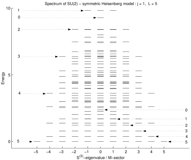
Figure 1: The spectrum of a ferromagnetic Heisenberg chain consisting of $5$ spin-$1$ spins with constant couplings. On the horizontal axis we have plottted the eigenvalue of the third component of the total spin. The spectrum is off-set so that the ground state energy vanishes. The arrows on the right, with label $S$, indicate the multiplets of eigenvalues $E(H,S)$, i.e., the smallest eigenvalue in the subspace of total spin $S$. The monotone ordering of the spin labels is the FOEL property. On the left, we have indicated the largest eigenvalues for each value of the total spin. The monotone ordering of their labels in the range $1,\ldots,5$, is the content of the Lieb-Mattis theorem [17] applied to this system.

In [17], Lieb and Mattis proved ordering of energy levels for a class of Heisenberg models on bipartite graphs, which includes the standard antiferromagnetic Heisenberg model. The FOEL property mentioned above can be considered as the ferromagnetic counterpart. To compare, a bipartite graph $G=(V,E)$ is a graph such that its set of vertices $V$ has a partition $V=A\cup B$ where $A\cap B=\emptyset$ and and any edge $(xy)\in E$ satisfies either $x\in A$ and $y\in B$, or $x\in B$ and $y\in A$. For such a graph, one considers Hamiltonians of the form

$$H=-H_{V}+H_{A}+H_{B},$$

where $H_{V},H_{A}$, and $H_{B}$ are ferromagnetic Heisenberg Hamiltonians on the graph $G$, and arbirary graphs $A$ and $B$, respectively. Let $S_{X}=\sum_{x\in X}s_{x}$, for $X=A,B,V$. The Lieb-Mattis Theorem [17, 18] then states that

(i) the ground state energy of $H$ is $E(H,|S_{A}-S_{B}|)$

(ii) if $|S_{A}-S_{B}|\leq S<S^{\prime}$, then $E(H,S)<E(H,S^{\prime})$.

One can see this property illustrated in Figure 1.

We first obtained a proof of FOEL for the spin 1/2 chain in [25]. In that paper we also prove the same result for the ferromagnetic XXZ chain with $SU_{q}(2)$ symmetry. Later, in [27], we generalized the result to chains with arbitray values of the spin magnitudes $s_{x}$ and coupling constants $J_{x,x+1}>0$. In short, we have the following theorem.

Theorem 4.2

FOEL holds for all ferromagnetic chains.

The main tool in the proof is a special basis of SU(2) highest weight vectors introduced by Temperley-Lieb [31] in the spin 1/2 case and by Frenkel and Khovanov [11] in the case of arbitrary spin. Some generalizations beyond the standard Heisenberg model have been announced [27, 28].

The FOEL property has a number of interesting consequences. The first immediate implication of FOEL is that the ground state energy of $H$ is $E(H,S_{\rm max})$, corresponding to the well-know fact that the ground state space coincides with the subspace of maximal total spin. Since there is only one multiplet of total spin $S_{\rm max}$, FOEL also implies that the gap above the ground state is $E(H,S_{\rm max}-1)-E(H,S_{\rm max})$. In the case of translation invariant models this is the physically expected property that the lowest excitations are simple spin-waves.

Another application of the FOEL property arises from the unitary equivalence of the Heisenberg Hamiltonian and the generator of the Symmetric Simple Exclusion Process (SSEP). To be precise, let $G=(V,E)$ be any finite graph, and define $\Omega_{n}$ to be the configuration space of $n$ particles, for $n=0,1,\ldots,|V|$, consisting of $\eta:V\to\{0,1\}$, with $\sum_{x\in V}\eta(x)=n$. For any $(xy)\in E$, let $r_{xy}>0$. The SSEP is the continuous time Markov process on $\Omega_{n}$ which exchanges the states (whether there is a particle or not) at $x$ and $y$ with rate $r_{xy}$, independently for each edge $(xy)$. The case $n=1$ is the random walk on $G$ with the given rates.

Alternatively, this process is defined by its generator on $l^{2}(\Omega_{n})$:

$$Lf(\eta)=\sum_{(xy)\in E}r_{xy}(f(\eta)-f(\eta^{xy})),$$

where $\eta^{xy}$ is the configuration $\eta$ with the values at $x$ and $y$ interchanged. One verifies $L\geq 0$, $L1=0$, and therefore $L$ generates a Markov semigroup $\{e^{-tL}\}_{t\geq 0}$, such that

$$\int f(\eta)\mu_{t}(d\eta)=\int(e^{-tL}f)(\eta)\mu_{0}(d\eta)\quad.$$

where $\mu_{0}$ is the initial probability distribution on the particle configurations. It is easy to show that for each $n$ there is a unique stationary measure given by the uniform distribution on $\Omega_{n}$. The relaxation time, which determines the exponential rate of convergence to the stationary state, is given by $1/\lambda(n)$, where $\lambda(n)>0$ is the spectral gap (smallest eigenvalue $>0$) of $L$ as an operator on $l^{2}(\Omega_{n})$.

Aldous, based on discussions with Diaconis [2], made the following remarkable conjecture concerning $\lambda(n)$:

Conjecture 4.3 (Aldous)

$\lambda(n)=\lambda(1)$, for all $1\leq n\leq|V|-1$.

Assuming the conjecture, one may determine the gap by solving the one-particle problem.

To make the connection with FOEL, observe

$$\bigoplus_{n=0}^{|V|}l^{2}(\Omega_{n})\cong({\mathbb{C}}^{2})^{\otimes|V|}\equiv{\mathcal{H}}_{V}$$

This is the Hilbert space of a spin 1/2 model on $V$. An explicit isomorphism is given by

$$f\mapsto\psi=\sum_{\eta}f(\eta)\left|\eta\right\rangle,$$

where $\left|\eta\right\rangle\in{\mathcal{H}}$ is the tensor product basis vector defined by

$$S^{3}_{x}\left|\eta\right\rangle=(\eta_{x}-1/2)\left|\eta\right\rangle$$

Under this isomorphism the generator, $L$, of the SSEP becomes the XXX Hamiltonian $H$. To see this it suffices to calculate the action of $L$:

$$Lf(\eta) \mapsto \sum_{\eta}(Lf)(\eta)\left|\eta\right\rangle$$

$$= \sum_{(xy)}\sum_{\eta}r_{xy}(f(\eta)-f(\eta^{xy}))\left|\eta\right\rangle$$

$$= \sum_{(xy)}\sum_{\eta}r_{xy}(1-t_{xy})f(\eta)\left|\eta\right\rangle$$

$$= H\psi$$

where $t_{xy}$ is the unitary operator that interchanges the states at $x$ and $y$, and the last step uses

$$1/2-2\boldsymbol{S}_{x}\cdot\boldsymbol{S}_{y}=1-t_{xy},$$

and $J_{xy}=2r_{xy}$.

The number of particles, $n$, is a conserved quantity for SSEP. Since, $S^{3}_{\rm tot}=-|V|/2+n$, the corresponding conserved quantity for the Heisenberg model is the third component of the total spin. Under the isomorphism the invariant subspace of all functions $f$ supported on $n$-particle configurations is identified with the set of vectors with $S^{3}=S^{3}_{\rm max}-n$, which we will denote by ${\mathcal{H}}_{n}$. The unique invariant measure of SSEP for $n$ particles on $V$, which is the uniform measure, corresponds to the ferromagnetic ground state with magnetization $n-|V|/2$. The eigenvalue $\lambda(n)$ is the spectral gap of $H_{V}|_{{\mathcal{H}}_{n}}$. It is then easy to see that the FOEL property implies that $\lambda(n)=\lambda(1)$. Since we proved FOEL for chains, we also provided a new proof of Aldous’ Conjecture in that case [12].

5 Droplet Excitations of the XXZ Chain

The low-lying excitations of the ferromagnetic XXZ chain describe droplets, i.e., domains of opposite magnetization [26]. This is to be contrasted with the situation for the antiferromagnetic XXZ chain. For the antiferromagnetic chain it has been proven that the low-energy spectrum does not contain droplet states; states with an antiferromagnetically ordered domain which is out of phase with its surroundings [7, 21]. In the following we only discuss the ferromagnetic chain.

Kennedy calculated the droplet energies as a function of the quasi-momentum. He obtained a Fourier series with coefficients that are a power series in $1/\Delta$ [15].

By combining the Bethe Ansatz with the representation of the XXZ Hamiltonian in the Temperley-Lieb basis employed to prove FOEL, it has been possible to obtain more detailed information about the location and width of the energy band comprised of the droplet states [24].

To state the new results we first need to introduce the $SU_{q}(2)$-symmetric XXZ chain [29]. Consider the spin 1/2 chain with boundary fields as defined by the following Hamiltonian:

$$H_{L} = -\sum_{x=1}^{L-1}J[\Delta^{-1}(S^{1}_{x}S^{1}_{x+1}+S^{2}_{x}S^{2}_{x+1})+(S_{x}^{3}S_{x+1}^{3}-1/4)]$$

$$-A(\Delta)(S_{L}^{3}-S^{3}_{1}).$$

where, $J>0$, $\Delta>1$, and $A(\Delta)=\frac{1}{2}\sqrt{1-1/\Delta^{2}}$. This model commutes with $SU_{q}(2)$, with $q\in(0,1)$ such that $\Delta=(q+q^{-1})/2$. The generators of this symmetry are:

$$S^{3}\! = \!\sum_{x=1}^{L}{\mathchoice{\mathrm{1\mskip-4.0mul}}{\mathrm{1\mskip-4.0mul}}{\mathrm{1\mskip-4.5mul}}{\mathrm{1\mskip-5.0mul}}}_{1}\otimes\cdots\otimes S^{3}_{x}\otimes{\mathchoice{\mathrm{1\mskip-4.0mul}}{\mathrm{1\mskip-4.0mul}}{\mathrm{1\mskip-4.5mul}}{\mathrm{1\mskip-5.0mul}}}_{x+1}\otimes\cdots{\mathchoice{\mathrm{1\mskip-4.0mul}}{\mathrm{1\mskip-4.0mul}}{\mathrm{1\mskip-4.5mul}}{\mathrm{1\mskip-5.0mul}}}_{L}$$

$$S^{+}\! = \!\sum_{x=1}^{L}t_{1}\otimes\cdots\otimes t_{x-1}\otimes S^{+}_{x}\otimes{\mathchoice{\mathrm{1\mskip-4.0mul}}{\mathrm{1\mskip-4.0mul}}{\mathrm{1\mskip-4.5mul}}{\mathrm{1\mskip-5.0mul}}}_{x+1}\otimes\cdots{\mathchoice{\mathrm{1\mskip-4.0mul}}{\mathrm{1\mskip-4.0mul}}{\mathrm{1\mskip-4.5mul}}{\mathrm{1\mskip-5.0mul}}}_{L}$$

$$S^{-}\! = \!\sum_{x=1}^{L}{\mathchoice{\mathrm{1\mskip-4.0mul}}{\mathrm{1\mskip-4.0mul}}{\mathrm{1\mskip-4.5mul}}{\mathrm{1\mskip-5.0mul}}}_{1}\otimes\cdots\otimes S^{-}_{x}\otimes t^{-1}_{x+1}\otimes\cdots t^{-1}_{L}$$

where

$$t_{x}=\left(\begin{array}[]{cc}q^{-1}&0\\ 0&q\end{array}\right)\,,\quad[S^{+},S^{-}]=\frac{q^{2S^{3}}-q^{-2S^{3}}}{q-q^{-1}}\,.$$

The Hamiltonian $H_{L}$ also commutes with the Casimir opeator for $SU_{q}(2)$, given by

$$C=S^{+}S^{-}+\frac{(qT)^{-1}+qT}{(q^{-1}-q)^{2}},\quad T=t_{1}\otimes t_{2}\otimes\cdots\otimes t_{L}.$$

The eigenvalues of $C$ are

$$\frac{q^{-(2S+1)}+q^{2S+1}}{(q^{-1}-q)^{2}},\quad S=0,1/2,1,3/2,\ldots$$

and play the same role as $S$ for the XXX model, e.g., they label the irreducible representations of $SU_{q}(2)$.

The FOEL property with respect to $S$, as defined in Section 4, can be proved in the same way as before [25]:

$$E(H_{L},S+1)<E(H_{L},S).$$

It is rather natural to ask what the states with minimal energy for given $S$ describe. It will be convenient to express $S$ by its deviation from the maximum possible value, i.e., $n$ such that $S=S_{\rm max}-n$. The answer is that $E(H_{L},S_{\rm max}-n)$, is the ground state energy of a droplet of $n$ down spins in a background of up spins. By the quantum group symmetry this is necessarily also the energy of a state in which a kink and a droplet coexist. In the thermodynamic limit the quantum symmetry evaporates, at least in the ground state representation [9], but some traces remain. In particular, the droplet energies computed in the $SU_{q}(2)$-symmetric model give the correct droplet energy in thermodynamic limit computed with periodic boundary conditions. To state this precisely, define $E_{L}(n)=\inf\mathop{\rm spec}H^{\rm periodic}_{L}|_{{\mathcal{H}}_{n}}$, where ${\mathcal{H}}_{n}$ is the eigenspace of $S^{3}$ with eigenvalue $S^{3}_{\rm max}-n$. The following theorem is proved in [24]:

Theorem 5.1

$$\lim_{L\to\infty}E(H_{L},S_{\rm max}-n)=\lim_{L\to\infty}E_{L}(n)=E(n)\equiv\frac{(1-q^{2})(1-q^{n})}{(1+q^{2})(1+q^{n})}.$$

The value of $E(n)$ itself is calculated by a simple version of the Bethe Ansatz. To make the calculation rigorous, we rely on positivity properties of the Hamiltonian in suitable bases. One can further show that $E(n)$ belongs to the continuous spectrum and is the bottom of a band of width

$$4q^{n}\frac{1-q^{2}}{1-q^{2n}}.$$

The states corresponding to this band can be interpreted as a droplet of size $n$ with a definite momentum. If we consider the droplet as a particle, the formula for the width indicates that the “mass” of the particle diverges as $n\to\infty$.

The energy $E(n)$ was considered by Yang and Yang in their famous series of papers on the XXZ chain [32]. However, due to an error, they got an energy of order $n$, which prevented the interpretation of the states as droplet states.

Acknowledgement. This work was supported in part by the National Science Foundation under Grant # DMS-0303316.

References

- [1] I. Affleck, T. Kennedy, E.H. Lieb, and H. Tasaki, Valence bond ground states in isotropic quantum antiferromagnets, Comm. Math. Phys. 115 (1987), 477–528.
- [2] D. Aldous, http://stat-www.berkeley.edu/users/aldous/problems.ps.
- [3] C. Borgs, J. T. Chayes, and J. Fröhlich, Dobrushin states in quantum lattice systems, Comm. Math. Phys. 189 (1997), no. 2, 591–619.
- [4] C. Borgs, R. Kotecký, and D. Ueltschi, Low temperature phase diagrams for quantum perturbations of classical spin systems, Comm. Math. Phys. 181 (1996), no. 2, 409–446.
- [5] O. Bratteli and D.W. Robinson, Operator algebras and quantum statistical mechanics 2, second edition ed., Springer Verlag, 1997.
- [6] Nilanjana Datta, Roberto Fernández, and Jürg Fröhlich, Low-temperature phase diagrams of quantum lattice systems. I. Stability for quantum perturbations of classical systems with finitely-many ground states, J. Statist. Phys. 84 (1996), no. 3-4, 455–534.
- [7] Nilanjana Datta and Tom Kennedy, Instability of interfaces in the antiferromagnetic chain at zero temperature, Comm. Math. Phys. 236 (2003), no. 3, 477–511.
- [8] M. Fannes, B. Nachtergaele, and R. F. Werner, Finitely correlated states of quantum spin chains, Comm. Math. Phys. 144 (1992), 443–490.
- [9] , Quantum spin chains with quantum group symmetry, Comm. Math. Phys. 174 (1996), 477–507.
- [10] K. Fredenhagen, A remark on the cluster theorem, Comm. Math. Phys. 97 (1985), 461–463.
- [11] I. B. Frenkel and M. G. Khovanov, Canonical bases in tensor products and graphical calculus for , Duke Math. J. 87 (1997), 409–480.
- [12] S. Handjani and D. Jungreis, Rate of convergence for shuffling cards by transpositions, J. Theor. Prob. 9 (1996), 983–993.
- [13] M.B. Hastings, Lieb-schultz-mattis in higher dimensions, Phys. Rev. B 69 (2004), 104431.
- [14] M.B. Hastings and T. Koma, Spectral gap and exponential decay of correlations, arXiv:math-ph/0507008.
- [15] T. Kennedy, Expansions for droplet states in the ferromagnetic Heisenberg chain, Markov Process. Related Fields 11 (2005), no. 2, 223–236.
- [16] Tom Kennedy and Hal Tasaki, Hidden symmetry breaking and the Haldane phase in quantum spin chains, Comm. Math. Phys. 147 (1992), no. 3, 431–484.
- [17] E. Lieb and D. Mattis, Ordering energy levels of interacting spin systems, J. Math. Phys. 3 (1962), 749–751.
- [18] E.H. Lieb, Two theorems on the hubbard model, Phys. Rev. Lett. 62 (1989), 1201–1204.
- [19] E.H. Lieb and D.W. Robinson, The finite group velocity of quantum spin systems, Comm. Math. Phys. 28 (1972), 251–257.
- [20] T. Matsui, Quantum statistical mechanics and Feller semigroup, Quantum probability communications, QP-PQ, X, World Sci. Publishing, River Edge, NJ, 1998, pp. 101–123.
- [21] , On the absence of non-periodic ground states for the antiferromagnetic model, Comm. Math. Phys. 253 (2005), no. 3, 585–609.
- [22] B. Nachtergaele, The spectral gap for some quantum spin chains with discrete symmetry breaking, Comm. Math. Phys. 175 (1996), 565–606, arXiv:cond-mat/9410110.
- [23] B. Nachtergaele and R. Sims, Lieb-robinson bounds and the exponential clustering theorem, arXiv:math-ph/0506030.
- [24] B. Nachtergaele, W. Spitzer, and S. Starr, Droplet excitations for the spin-1/2 xxz chain with kink boundary conditions, arXiv:math-ph/0508049.
- [25] , Ferromagnetic ordering of energy levels, J. Stat. Phys. 116 (2004), 719–738, arXiv:math-ph/0308006.
- [26] B. Nachtergaele and S. Starr, Droplet states in the XXZ Heisenberg model, Comm. Math. Phys. 218 (2001), 569–607, arXiv:math-ph/0009002.
- [27] , Ferromagnetic Lieb-Mattis theorem, Phys. Rev. Lett. 94 (2005), 057206, arXiv:math-ph/0408020.
- [28] , Ordering of energy levels in heisenberg models and applications, to appear in the proceedings of QMATH9, Giens, September 2004, 2005, arXiv:math-ph/0503056.
- [29] V. Pasquier and H. Saleur, Common structures between finite systems and conformal field theories through quantum groups, Nuclear Physics B 330 (1990), 523–556.
- [30] B. Simon, The statistical mechanics of lattice gases, Princeton University Press, 1993.
- [31] H. N. V. Temperley and E. H. Lieb, Relations between the ‘percolation’ and ‘colouring’ problem and other graph-theoretical problems associated with regular planar lattices: some exact results for the ‘percolation’ problem, Proc. Roy. Soc. A322 (1971), 252–280.
- [32] C.N. Yang and C.P. Yang, One-dimensional chain of anisotropic spin-spin interactions. iii. applications, Phys. Rev. 151 (1966), 258–264.
- [33] D. A. Yarotsky, Ground states in relatively bounded quantum perturbations of classical lattice systems, arXiv:math-ph/0412040.