Abstract

We discuss magnetic Schrödinger operators perturbed by measures from the generalized Kato class. Using an explicit Krein-like formula for their resolvent, we prove that these operators can be approximated in the strong resolvent sense by magnetic Schrödinger operators with point potentials. Since the spectral problem of the latter operators is solvable, one in fact gets an alternative way to calculate discrete spectra; we illustrate it by numerical calculations in the case when the potential is supported by a circle.

1 Introduction

Schrödinger operators are used for modelling a particle confined in a quantum-mechanical system. Depending on a potential which describes how the particle interacts with its environment, one can consider a wide range of physical situations. In this paper, we are particularly interested in potentials in dimension two supported by zero measure sets; the supports could be for example graphs, curves or points.

The motivation to study such operators is based on the fact that they represent simple mathematical models of various nano-structures like quantum wires, photonic crystals, quantum dots, etc. One possible way to describe them is via quantum graphs; it means that one considers ordinary differential equations on the graph edges, which are coupled through boundary conditions at the graph vertices so that the resulting operator is self-adjoint, see [K] or [KS]. The operators we are going to deal with yield an alternative approach. The particle is not confined to the graph, but it moves in its vicinity if the potentials are attractive. Hence the latter model is in a sense more realistic and it enables us to take the tunnelling effect into account.

We aim to prove a limit relation between two classes of operators in $L^{2}(\mathbb{R}^{2})$ in the presence of a magnetic field: those with attractive potentials supported by a curve or a graph on one side, and operators with point potentials on the other side. The crucial feature of the latter operators is the solvability of their spectral problem; if the number of potentials is finite, then the essential spectrum stays unchanged and the discrete spectrum can be calculated numerically by solving an implicit equation. Therefore, if we are able to find a sequence of point potential operators which approximates the given operator, we get an approximate method to calculate its discrete spectrum.

In fact, we will show that the approximation works for a larger family of potentials than just the ones supported by a curve. The regular potentials with Kato property will be also included; that is why we speak about a generalized Kato class and potentials are replaced by more general measures. For a given measure $m$ from the generalized Kato class, it is possible to define the operator $-\Delta+m$ via association with a closed and semi-bounded quadratic form, see e.g. [BEKŠ] and [SV]. The second way to define Schrödinger operators with potentials supported by zero measure sets is by prescribing the operator domains, see [Po1] for general singular perturbations, and [AGHH] or [GHS] for point potentials; there the domains are given by imposing a boundary condition on wavefunctions.

It was shown in [BFT] that the free Laplacian perturbed by a measure with Kato property can be approximated by point potential operators; in dimension one the convergence is in the norm resolvent sense, while in dimension three it is in the strong resolvent sense. According to [EN2], the situation in dimension two is similar to the three-dimensional case, moreover, the authors presented several physical systems where the approximation is useful in spectral calculations.

The present task is to prove that the approximation also works in the presence of a magnetic field. It turns out that the main difficulty is not the proof itself (it easily carries over from the non-magnetic case) but rather the lack of information about magnetic systems. Namely, we first need to clarify the definition of perturbations by a measure in section 3. Then in section 4 we derive an explicit formula for resolvents; that must be done without using results from [BEKŠ] directly because their proof relies on the positivity preserving property of the free Laplacian. Section 5 deals with point potentials in the presence of a magnetic field. Finally, in section 6 we state the main approximation claim and we apply the approximation to a simple example in section 7, where the magnetic field is homogeneous and the potential is supported a circle.

2 Magnetic Schrödinger operator in $\mathbb{R}^{2}$

The free magnetic Schrödinger operator on $L^{2}(\mathbb{R}^{2})$ is given by

$$(-{\rm i}\nabla-A(x))^{2},$$

where $A(x)$ is a vector potential, whose components $A_{1}$ and $A_{2}$ belong to $C^{\infty}(\mathbb{R}^{2})$. According to [CFKS, chapter 1.3], there exists a closed and positive quadratic form $h$,

$$D(h) = \left\{\psi\in L^{2}(\mathbb{R}^{2}):\;(\partial_{j}-iA_{j})\psi\in L^{2}(\mathbb{R}^{2}),\;j=1,2\right\}$$

$$h(\varphi,\psi) = \sum_{j=1}^{2}((\partial_{j}-iA_{j})\varphi,(\partial_{j}-iA_{j})\psi)_{L^{2}(\mathbb{R}^{2})}.$$

We define the free magnetic Schrödinger operator $H_{0}$ as the unique self-adjoint operator associated with the form $h$, i.e.

$$D(H_{0}) \subset D(h)$$

$$(H_{0}\varphi,\psi) = h(\varphi,\psi)\qquad\varphi,\psi\in D(H_{0}).$$

Moreover, from [CFKS, theorem 1.13] we know that $C^{\infty}_{0}(\mathbb{R}^{2})$ is a form core of $H_{0}$.

By [BGP1, theorem 14] the resolvent $(H_{0}-z)^{-1}$ has an integral kernel $G_{0}(x,y;z)$ which is continuous away from the diagonal $x=y$. The singularity of $G_{0}(x,y;z)$ on the diagonal is of the same type as the one for the non-magnetic Green function; following [BGP2, theorem 15], it can be rewritten as

$$G_{0}(x,y;z)=-{1\over 2\pi}\,\ln(|x-y|)+G_{0}^{\mathrm{ren}}(x,y;z),$$

where $G_{0}^{\mathrm{ren}}(\cdot;z)$ is continuous on $\mathbb{R}^{2}\times\mathbb{R}^{2}$. Hence it is possible to introduce the regularized Green function

$$\xi(a;z)=\lim_{|x-a|\to 0}\left[G_{0}(x,a;z)+{1\over 2\pi}\,\ln(|x-y|)\right]=G_{0}^{\mathrm{ren}}(a,a;z).$$ (1)

We will need this function when defining a perturbation by point potentials.

In the special case of a homogeneous magnetic field $B$ one can write Green function $G_{0}(z)$ explicitly. For example, in the symmetric gauge, $A(x)=(-{1\over 2}Bx_{2},{1\over 2}Bx_{1})$, $B\in\mathbb{R}$, Green function has the following form, see [DMM]

$$G_{0}(x,y;z)={1\over 4\pi}\,\Phi_{B}(x,y)\,\Gamma\left({|B|-z\over 2|B|}\right)U\left({|B|-z\over 2|B|},1;{|B|\over 2}|x-y|^{2}\right),$$ (2)

$U$ is the irregular confluent hypergeometric function [AS, 13.1.33] and $\Phi_{B}$ is a phase factor

$$\Phi_{B}(x,y)=\exp\left[-{{\rm i}B\over 2}(x_{1}y_{2}-x_{2}y_{1})-{|B|\over 4}|x-y|^{2}\right].$$

3 Perturbation by a measure

Next, we perturb the magnetic Hamiltonian $H_{0}$ by a measure $-\gamma m$ in the following way,

$$H_{\gamma m}=H_{0}-\gamma m,$$

where $m$ is a finite positive measure from generalized Kato class, which means in dimension two that it satisfies

$$\lim_{\varepsilon\to 0}\sup_{x\in\mathbb{R}^{2}}\int_{B(x,\varepsilon)}|\ln(|x-y|)|\,m(dy)=0,$$

with $B(x,\varepsilon)$ denoting the circle of radius $\varepsilon$ centred at $x$. $\gamma$ is a bounded and continuous function mapping $\Gamma:=\mathrm{supp}(m)$ into $\mathbb{R}_{+}$, thus we consider only attractive potentials. An example of such measure is the Dirac measure, supported by a curve or graph; one can easily check that the condition above holds.

By [SV, theorem 3.1] the potential generated by $m$ is ($-\Delta$)-form bounded with infinitesimally small relative bound. In order to define $H_{\gamma m}$ properly, we need a similar form-boundedness with respect to $H_{0}$. We cannot use the mentioned result directly as it was formulated only for Dirichlet quadratic forms, i.e. the ones which are positivity preserving. Instead, we can employ the diamagnetic inequality to pass from the non-magnetic system to the magnetic one. In the following, $\|\cdot\|_{p,q}$ denotes the norm of an operator acting from $L^{p}(\mathbb{R}^{2})$ to $L^{q}(\mathbb{R}^{2})$, $1\leq p,q\leq\infty$.

Lemma 1.

Let $m$ be a positive measure from the generalized Kato class w.r.t. $-\Delta$ and let $H_{0}$ be the self-adjoint operator defined above. Then for each $a>0$ there exists $b\in\mathbb{R}$ such that the following inequality holds for any $\psi\in C_{0}^{\infty}(\mathbb{R}^{2})$

$$\int_{\mathbb{R}^{2}}|\psi(x)|^{2}\,m(dx)\leq a\,h(\psi,\psi)+b\|\psi\|^{2}_{2}.$$ (3)

Proof: Since $m$ belongs to the generalized Kato class w.r.t. $-\Delta$, by [SV, theorem 3.1], the following inequality is fulfilled for any $\psi\in C^{\infty}_{0}(\mathbb{R}^{2})$

$$\int_{\mathbb{R}^{2}}|\psi(x)|^{2}\,m(dx)\leq\omega\left[\|\nabla\psi\|_{2}^{2}+\zeta\|\psi\|_{2}^{2}\right],$$ (4)

where according to [SV, remark 1.7(b)], $\omega:=\|(-\Delta+\zeta)^{-1}m\|_{\infty}$ and thus it decays with $\zeta$ growing to $+\infty$. It was proved by approximating $m$ by a sequence of non-negative potentials $V_{n}\in L^{2}(\mathbb{R}^{2})\cap L^{\infty}(\mathbb{R}^{2})$ such that

$$\lim_{n\to\infty}\int_{\mathbb{R}^{2}}|\psi(x)|^{2}\,V_{n}(x)\,dx=\int_{\mathbb{R}^{2}}|\psi(x)|^{2}\,m(dx)\qquad\forall\;\psi\in C_{0}^{\infty}(\mathbb{R}^{2}).$$

[SV, theorem 2.1] states that such sequence exists, $\|(-\Delta+\zeta)^{-1}V_{n}\|_{\infty,\infty}\leq\omega$, $n\in\mathbb{N}$ and inequality (4) holds also when $m(dx)$ is replaced by $V_{n}(x)\,dx$.

Let us write

$$\int_{\mathbb{R}^{2}}|\psi(x)|^{2}\,V_{n}(x)\,dx = \|V^{{1\over 2}}_{n}(H_{0}+\zeta)^{-{1\over 2}}(H_{0}+\zeta)^{{1\over 2}}\psi\|_{2}^{2}$$

$$\leq \|V^{{1\over 2}}_{n}(H_{0}+\zeta)^{-{1\over 2}}\|^{2}_{2,2}\left[h(\psi,\psi)+\zeta(\psi,\psi)\right].$$

Repeating the proof of [AHS, theorem 2.5], we make use of the diamagnetic inequality [HSU] in this form

$$\left|{\rm e}{-tH_{0}}\psi\right|\leq{\rm e}{-t(-\Delta)}|\psi|\qquad t>0,\;\psi\in L^{2}(\mathbb{R}^{2}).$$

Then from the expression

$$(H_{0}+\zeta)^{-{1\over 2}}={1\over\Gamma\left({1\over 2}\right)}\int t^{-{1\over 2}}{\rm e}{-t\zeta}{\rm e}{-tH_{0}}\;dt$$

we get $|(H_{0}+\zeta)^{-{1\over 2}}\psi|\leq(-\Delta+\zeta)^{-{1\over 2}}|\psi|$, which in turn yields

$$\|V^{{1\over 2}}_{n}(H_{0}+\zeta)^{-{1\over 2}}\|^{2}_{2,2}\leq\|V^{{1\over 2}}_{n}(-\Delta+\zeta)^{-{1\over 2}}\|^{2}_{2,2}\leq\|V_{n}^{{1\over 2}}(-\Delta+\zeta)^{-1}V_{n}^{{1\over 2}}\|_{2,2}.$$

The Stein interpolation theorem [RS, theorem IX.21] and the duality between $\|\cdot\|_{1,1}$ and $\|\cdot\|_{\infty,\infty}$ imply

$$\|V^{{1\over 2}}_{n}(H_{0}+\zeta)^{-{1\over 2}}\|^{2}_{2,2}\leq\|V_{n}(-\Delta+\zeta)^{-1}\|_{1,1}^{{1\over 2}}\|(-\Delta+\zeta)^{-1}V_{n}\|_{\infty,\infty}^{{1\over 2}}\leq\omega.$$

Finally, the convergence of $V_{n}$ to $m$ and the fact that $\omega\to 0$ as $\zeta\to\infty$ finish the proof. ∎

Since $C_{0}^{\infty}(\mathbb{R}^{2})$ is dense in $D(h)$ it is possible to define linear operator $I_{m}$

$$I_{m}\,:\;D(h)\mapsto L^{2}(m):=L^{2}(\mathbb{R}^{2},m)$$

$$I_{m}\psi=\psi\qquad\forall\psi\in C_{0}^{\infty}(\mathbb{R}^{2}).$$

Then (3) can be extended to whole $D(h)$ with function $\psi$ on the lhs being replaced by $I_{m}\psi$ and thus $I_{m}$ is bounded. Now, consider quadratic form $h_{\gamma m}$ given by

$$D(h_{\gamma m}) = D(h)$$

$$h_{\gamma m}(\psi,\varphi) = \int_{\mathbb{R}^{2}}(\nabla\bar{\psi}(x)+{\rm i}A(x)\,\bar{\psi}(x)).(\nabla\varphi(x)-{\rm i}A(x)\,\varphi(x))\,dx$$

$$-\int_{\mathbb{R}^{2}}I_{m}\bar{\psi}(x)\,I_{m}\varphi(x)\,\gamma(x)\,m(dx),$$

We employ the KLMN theorem, see [RS, theorem X.17], to conclude that $h_{\gamma m}$ is lower semi-bounded and closed. Thus there exists a unique self-adjoint operator $H_{\gamma m}$ associated with this form.

The definition that we have presented above applies to both regular potentials $m(dx)=V(x)dx$ and potentials supported by zero measure sets $\Gamma$. In the latter case there is an alternative way to define operator $H_{\gamma m}$ via boundary conditions. Consider an operator which behaves as $H_{0}$ away from the set $\Gamma$

$$\dot{H}_{\gamma m}\psi(x)=(-{\rm i}\nabla-A)^{2}\,\psi(x)\qquad x\in\mathbb{R}^{2}\setminus\Gamma$$

with the domain consisting of functions $\psi$ such that $H_{0}\psi\in L^{2}(\mathbb{R}^{2}\setminus\Gamma)$, their restriction to $\mathbb{R}^{2}\setminus\Gamma$ is smooth and which are moreover continuous at $\Gamma$ and have a jump in the normal (w.r.t. curve $\Gamma$) derivatives,

$${\partial\psi\over\partial n_{+}}(x)-{\partial\psi\over\partial n_{-}}(x)=-\gamma(x)\,\psi(x)\,,\qquad x\in\Gamma\,.$$

One can check that $\dot{H}_{\gamma m}$ is e.s.a. and by Green’s formula we have $(\dot{H}_{\gamma m}\psi,g)=h_{\gamma m}(\psi,g)$ for all $\psi\in D(\dot{H}_{\gamma m})$ and $g\in C^{\infty}_{0}(\mathbb{R}^{2})$. Since $C^{\infty}_{0}(\mathbb{R}^{2})$ is a core of $h_{\gamma m}$, the closure of $\dot{H}_{\gamma m}$ can be identified with $H_{\gamma m}$. This definition is applicable to curves $\Gamma$ which do not have any cusps and only a finite number of smooth edges meet in a node.

4 Krein-like formula

Throughout this work, a crucial role will be played by Krein’s formula which gives us an explicit expression for the resolvent of $H_{\gamma m}$. Originally, the formula was used for Hamiltonians perturbed by a finite number of point interactions, later, it was generalized to a large family of operators, see e.g. [Po1].

In paper [BEKŠ] the authors derived the resolvent for the free Laplacian perturbed by measure $m$ from generalized Kato class, using the positivity property of Green function of the Laplacian. Although their proof does not apply to magnetic systems, one would still expect that the resolvent corresponding to the operator $H_{0}$ with perturbed by $m$ should look the same in the presence of a magnetic field:

$$R(z)=R_{0}(z)+R_{dx,m}(z)\left[{1\over\gamma}-R_{m,m}(z)\right]^{-1}R_{m,dx}(z),$$ (5)

where $R_{\mu,\nu}(z)$ is an integral operator acting from $L^{2}(\mathbb{R}^{2},\nu)$ to $L^{2}(\mathbb{R}^{2},\mu)$, $\mu$ and $\nu$ are two arbitrary positive Radon measures and

$$R_{\mu,\nu}(z)\psi(x)=\int G_{0}(x,y;z)\,\psi(y)\,\nu(dy)\qquad\mu-\mathrm{a.e.}$$

Note that $R_{m,dx}(z)=I_{m}R_{0}(z)$.

To prove that (5) is indeed the resolvent of $H_{\gamma m}$, we first show several auxiliary results.

Lemma 2.

Assume that measure $m$ is finite, i.e. $\int m(dx)=l_{m}<\infty$ and $z\in\rho(H_{0})$. Then $R_{dx,m}(\bar{z})=(R_{m,dx}(z))^{*}$.

Proof: For $z\in\rho(H_{0})$ the operator $R_{m,dx}(z)$ is bounded and so is its adjoint. We have to check that in the expression

$$I=(f,R_{m,dx}(z)\psi)_{L^{2}(m)}=\int m(dy)\int dx\,\bar{f}(y)\,G_{0}(y,x;z)\,\psi(x)$$

one can interchange the order of integration. This is possible if the following integral is finite

$$I\leq I_{1}:=\int\int m(dy)\,dx\,|f(y)|\,|G_{0}(y,x;z)|\,|\psi(x)|.$$

By Kato’s inequality (see [BGP1]) one has

$$|G_{0}(x,y;z)|\leq K(x,y;z)=K(x-y,0;z)\qquad{\mathrm{a}.e.}\;x,y,\in\mathbb{R}^{2}$$

for $z$ sufficiently large negative, $K$ is the Green function of the free Laplacian $-\Delta$ in $L^{2}(\mathbb{R}^{2})$. Thus $I_{1}$ is dominated by $\|\psi\|_{L^{2}(\mathbb{R}^{2})}\,l_{m}^{1/2}\,\|K(z)\|_{L^{2}(\mathbb{R}^{2})}\,\|f\|_{L^{2}(m)}$. Together with the observation $G_{0}(x,y;z)=\overline{G_{0}(y,x;\bar{z})}$ (which is a consequence of $G_{0}(z)$ being a Carleman kernel, see [BGP1, theorem 16] and [GMC, theorem 1]) it implies the claim for large negative $z$. For any other $z\in\varrho(H_{0})$, it follows from the first resolvent formula

$$R_{dx,m}(z)=R_{dx,m}(z_{0})+(z-z_{0})R_{0}(z)R_{dx,m}(z_{0}).$$

∎

Lemma 3.

Consider mappings $I_{m}$ and $R_{m,dx}(z)$ defined as above and let $z_{0}<0$ be such that

$$(\psi,\varphi)_{z_{0}}:=h(\psi,\varphi)-(z_{0}\psi,\varphi)$$

is an inner product in $D(h)$. (Recall that $h$ is lower semi-bounded and closed form, thus $D(h)$ with $(\cdot,\cdot)_{z_{0}}$ is a Hilbert space.) Then $I_{m}^{*}=(R_{m,dx}(z_{0}))^{*}$.

The lemma was proved in [B], let us present its proof for the sake of completeness.

Proof: As both operators $I_{m}$ and $R_{m,dx}(z_{0})$ are bounded, their adjoint operators are bounded, too. For any $f\in L^{2}(m)$ and $\psi\in L^{2}(\mathbb{R}^{2})$ we have

$$(\psi,I_{m}^{*}f)_{L^{2}(\mathbb{R}^{2})} = h(R_{0}(z_{0})\psi,I_{m}^{*}f)-(z_{0}R_{0}(z_{0})\psi,I_{m}^{*}f)_{L^{2}(\mathbb{R}^{2})}$$

$$= (R_{0}(z_{0})\psi,I_{m}^{*}f)_{z_{0}}=(I_{m}R_{0}(z_{0})\psi,f)_{L^{2}(m)}$$

$$= (R_{m,dx}(z_{0})\psi,f)_{L^{2}(m)}=(\psi,(R_{m,dx}(z_{0}))^{*}f)_{L^{2}(\mathbb{R}^{2})}.$$

In the first line, we have used the fact that $R_{0}(z_{0})$ is the resolvent corresponding to Hamiltonian $H_{0}$, associated with $h$. In the second line, we have simply employed the definition of adjoint operator $I_{m}^{*}$; since $I_{m}$ maps from $D(h)$ with the inner product $(\cdot,\cdot)_{z_{0}}$ to $L^{2}(m)$ it reads $(\phi,I^{*}_{m}f)_{z_{0}}=(I_{m}\phi,f)_{L^{2}(m)}$, $\phi\in D(h)$ and $f\in L^{2}(m)$. ∎

Lemma 4.

Assume $z\in\rho(H_{0})$ and $f\in L^{2}(m)$. Then $R_{dx,m}(z)f\in D(h)$ and

$$h(R_{dx,m}(z)f,\psi)-(zR_{dx,m}(z)f,\psi)_{L^{2}(\mathbb{R}^{2})}=(f,I_{m}\psi)_{L^{2}(m)}$$

for all $\psi\in D(h)$.

Proof: Using the first resolvent formula, one has

$$R_{dx,m}(z)f=R_{dx,m}(z_{0})f+(z-z_{0})R_{0}(z)R_{dx,m}(z_{0})f,$$

where $z_{0}$ is the same as in the previous lemma; then the first term equals $I_{m}^{*}f$ and hence it belongs to $D(h)$. Also the second term belongs to $D(h)$ as the free resolvent $R_{0}(z)$ maps to $D(H_{0})\subset D(h)$.

To prove the second claim we substitute $R_{dx,m}(z)f$ from the above formula and we use lemma 3,

$$h(R_{dx,m}(z)f,\psi)-(zR_{dx,m}(z)f,\psi)_{L^{2}(\mathbb{R}^{2})}=\phantom{AAAAAAAAAAAAAAAAA}$$

$$\phantom{A}=(R_{dx,m}(z_{0})f,\psi)_{z_{0}}-((z-z_{0})R_{dx,m}(z_{0})f,\psi)_{L^{2}(\mathbb{R}^{2})}$$

$$\phantom{A=}+h((z-z_{0})R_{0}(z)R_{dx,m}(z_{0})f,\psi)-(z(z-z_{0})R_{0}(z)R_{dx,m}(z_{0})f,\psi)_{L^{2}(\mathbb{R}^{2})}$$

$$\phantom{A}=(I_{m}^{*}f,\psi)_{z_{0}}-((z-z_{0})R_{dx,m}(z_{0})f,\psi)_{L^{2}(\mathbb{R}^{2})}$$

$$\phantom{A=}+((z-z_{0})R_{dx,m}(z_{0})f,\psi)_{L^{2}(\mathbb{R}^{2})}$$

$$\phantom{A}=(f,I_{m}\psi)_{L^{2}(m)}.\phantom{AAAAAAAAAAAAAAAAAAAAAAAAAAAAAAAA}\qed$$

Theorem 5.

Suppose that $1/\gamma-R_{m,m}(z)$ is invertible. Then $R(z)$ given by (5) is defined on $L^{2}(\mathbb{R}^{2})$ and it is the resolvent of $H_{\gamma m}$.

Proof: Take arbitrary $\psi\in L^{2}(\mathbb{R}^{2})$ and $\varphi\in D(h)$, then by lemma 4 and Krein’s formula (5) $R(z)\psi$ belongs to $D(h)$. We have to check that

$$I:=h_{\gamma m}(R(z)\psi,\varphi)-(zR(z)\psi,\varphi)_{L^{2}(\mathbb{R}^{2})}=(\psi,\varphi)_{L^{2}(\mathbb{R}^{2})}.$$

Denote $g=(1/\gamma-R_{m,m}(z))^{-1}R_{m,dx}(z)\psi$, then

$$I = h(R_{0}(z)\psi,\varphi)-(zR_{0}(z)\psi,\varphi)_{L^{2}(\mathbb{R}^{2})}-(I_{m}R_{0}(z)\psi,\gamma I_{m}\varphi)_{L^{2}(m)}$$

$$+ h(R_{dx,m}(z)g,\varphi)-(zR_{dx,m}(z)g,\varphi)_{L^{2}(\mathbb{R}^{2})}-(I_{m}R_{dx,m}(z)g,\gamma I_{m}\varphi)_{L^{2}(m)}$$

According to lemma 4, the fourth and fifth term give together $(g,I_{m}\varphi)_{L^{2}(m)}$, so one gets

$$I=(\psi,\varphi)_{L^{2}(\mathbb{R}^{2})}+\Big{(}-R_{m,dx}(z)\,\psi+{1\over\gamma}\,g-R_{m,m}(z)\,g,\gamma\,I_{m}\varphi\Big{)}_{L^{2}(m)},$$

finally, employing the definition of $g$ shows that the second term equals zero. ∎

One can fulfil the hypothesis that the operator $1/\gamma-R_{m,m}(z)$ is invertible easily by choosing sufficiently large negative $z$; it follows from the next lemma, see [BEKŠ, corollary 2.2]. In the following, $\|T\|_{p,q}$ denotes the norm of an operator $T$ acting from $L^{p}(m)$ to $L^{q}(m)$.

Lemma 6.

There exists $\tilde{z}<0$ such that $\|\gamma R_{m,m}(z)\|_{2,2}<1$ for all $z<\tilde{z}$.

Proof: Since the measure $m$ belongs to Kato class and $\gamma$ is bounded, we can find $0<a<1$ and $0<b<\infty$ such that

$$\int_{\mathbb{R}^{2}}|I_{m}\psi(x)|^{2}(1+\gamma(x)^{2})\,m(dx)\leq a\,h(\psi,\psi)+b\,(\psi,\psi)_{L^{2}(\mathbb{R}^{2})}$$

for all $\psi\in D(h)$. We put $\tilde{z}=-b/a$, the rhs of the inequality then reads

$$a\,(\psi,\psi)_{\tilde{z}}\,:=\,a\,h(\psi,\psi)-a\,(\tilde{z}\psi,\psi)_{L^{2}(\mathbb{R}^{2})}.$$

Next, we take any $f\in L^{2}(m)$ and $z<\tilde{z}$ and introduce a set

$$S_{z}:=\{\psi\in D(h):\;(\psi,\psi)_{z}=1\}.$$

Consequently, we have

$$\int_{\mathbb{R}^{2}}|I_{m}R_{dx,m}(z)f(x)|^{2}\,\gamma^{2}(x)\,m(dx)\leq a\,(R_{dx,m}(z)f,R_{dx,m}(z)f)_{z}\phantom{AAAAA}$$

$$\phantom{A}\leq a\sup_{\psi\in S_{z}}|(R_{dx,m}(z)f,\psi)_{z}|^{2}=a\sup_{\psi\in S_{z}}|(f,I_{m}\psi)_{L^{2}(m)}|^{2}$$

$$\phantom{A}\leq a\int|f(x)|^{2}\,m(dx)\sup_{\psi\in S_{z}}\int|I_{m}\psi(x)|^{2}\,m(dx)$$

$$\phantom{A}\leq a\,\|f\|^{2}_{L^{2}(m)}\,a\,(\psi,\psi)_{z}=a^{2}\,\|f\|^{2}_{L^{2}(m)}\phantom{AAAAAAAAAAAAAAAAAAAA}\qed$$

For further use we rewrite the Hamiltonian $H_{\gamma m}$ into the form $H_{0}-{1\over\alpha}\mu$, where

$$\mu={\gamma m\over\int\gamma m},\qquad\alpha={1\over\int\gamma m}.$$

Since both function $\gamma$ and measure $m$ are positive, the coupling constant $\alpha$ and normalized measure $\mu$ are positive, too. The resolvent $R(z)=(H_{\gamma m}-z)^{-1}$ then acts on arbitrary $\psi\in L^{2}(\mathbb{R}^{2})$ as follows

$$R(z)\psi=R_{0}(z)\psi+R_{dx,\mu}(z)[\alpha-R_{\mu,\mu}(z)]^{-1}R_{\mu,dx}(z)\psi.$$ (6)

According to lemma 6, $\|{1\over\alpha}R_{\mu,\mu}(z)\|_{2,2}$ is less than 1 for sufficiently large negative $z$, one can prove the same about the norm $\|\cdot\|_{\infty,\infty}$ using the Kato property of $\mu$. From now on we consider only large negative $z$ so that both norms above are less than 1. The second term on the rhs of (6) can be substituted by $R_{dx,\mu}(z)\sigma$, where $\sigma\in L^{2}(\mu)$ is the unique solution to the equation

$$[\alpha-R_{\mu,\mu}(z)]\sigma=R_{\mu,dx}(z)\psi\qquad\mu-\mathrm{a.e.}$$ (7)

By [BGP1, theorem 16] domain $D(H_{0})$ is embedded into the space of continuous and bounded function on $\mathbb{R}^{2}$, thus $R_{0}(z)\psi$ is bounded and continuous in $\mathbb{R}^{2}$ and the same is of course true for function $R_{\mu,dx}(z)\psi$ on $\Gamma$. Adding the information about norms of ${1\over\alpha}R_{\mu,\mu}(z)$, we may conclude that $\sigma$ is bounded and continuous on $\Gamma$ as well.

5 Point potentials

Next consider a magnetic Schrödinger operator $H_{Y,\alpha}$ with finitely many point potentials placed at points $a\in Y\subset\Gamma$, $|Y|$ denotes the number of potentials. The operator is defined via self-adjoint extensions; away from the points from $Y$ it behaves as the free operator $H_{0}$ and the wavefunctions from its domain must have following behaviour in the vicinity of each point $a\in Y$,

$$\psi(x)=\ln|x-a|L_{0}(\psi,a)+L_{1}(\psi,a)+{\cal O}(|x-a|)$$ (8)

with coefficients $L_{0}$ and $L_{1}$ fulfilling the boundary condition

$$L_{1}(\psi,a)+2\pi\alpha(a)L_{0}(\psi,a)=0\qquad\forall a\in Y.$$

For further details concerning point potentials see e.g. [AGHH] for the non-magnetic case and [GHS] for the magnetic case. In general, one can choose any real number $\alpha(a)$ for each potential independently, here, we make a special choice $\alpha(a)=\alpha|Y|$ for all $a\in Y$, with $\alpha$ defined in the previous subsection.

The resolvent $(H_{Y,\alpha}-z)^{-1}$ is given by Krein’s formula,

$$(H_{Y,\alpha}-z)^{-1}\psi\,(x)=R_{0}(z)\psi\,(x)+\sum_{y,y^{\prime}\in Y}[\Lambda_{Y,\alpha}(z)]^{-1}(y,y^{\prime})\,G_{0}(x,y;z)\,R_{0}(z)\psi\,(y^{\prime}),$$ (9)

where $\Lambda_{Y,\alpha}(z)$ is a matrix $|Y|\times|Y|$,

$$\Lambda_{yy^{\prime}}=\left\{\begin{array}[]{ll}|Y|\alpha-\xi(y;z)&y=y^{\prime}\\ -G_{0}(y,y^{\prime};z)&y\neq y^{\prime},\end{array}\right.$$

$\xi(y;z)$ is the regularized Green function (1). For a homogeneous magnetic field $B$, we can calculate $\xi(a;z)$ explicitly; it does not depend on the potential position $y$ and it equals $-{1\over 4\pi}\left[\psi\left({|B|-z\over 2|B|}\right)+2C_{E}+\ln\left({|B|\over 2}\right)\right]$, with $C_{E}$ denoting the Euler constant. The second term on the rhs of (9) can be rewritten as $\sum_{y\in Y}G_{0}(x,y;z)q_{y}$, where $q$ is the $|Y|$-dimensional vector which solves

$$R_{0}(z)\psi\,(y)=\sum_{y^{\prime}\in Y}(\Lambda_{Y,\alpha}(z))(y,y^{\prime})q_{y^{\prime}}\qquad\forall\;y\in Y.$$ (11)

One possible way to make matrix $\Lambda$ invertible is to take a sufficiently large set $Y$.

Lemma 7.

Let $Y_{n}$ be a sequence of subsets of $\Gamma$ with $|Y_{n}|\to\infty$ as $n\to\infty$, and assume that for some $\tilde{\alpha}<\alpha$ we have

$$\sup_{n\in\mathbb{N}}{1\over|Y_{n}|}\sup_{x\in Y_{n}}\sum_{y\in Y_{n}\setminus\{x\}}|G_{0}(x,y;z)|\leq\tilde{\alpha}<\alpha.$$

Then there exist $C>0$ and $n_{0}\in\mathbb{N}$ such that $\Lambda_{Y_{n},\alpha}(z)$ is invertible and

$$\left\|\left({1\over|Y_{n}|}\Lambda_{Y_{n},\alpha}(z)\right)^{-1}\right\|_{2,2}<C$$

for all $n\geq n_{0}$.

Here and in the following section, the symbol $\|T\|_{p,q}$ denotes the operator norm of a matrix $T$, acting from $\ell^{p}(Y)$ to $\ell^{q}(Y)$ and correspondingly, $\|\cdot\|_{p}$ is the norm in $\ell^{p}(Y)$.

Proof: Let us split matrix $\Lambda_{Y_{n},\alpha}(z)/|Y_{n}|$ into the diagonal and non-diagonal part. On the diagonal, $\xi(\cdot;z)$ stays bounded because it is a continuous function on a compact set $\Gamma$. Therefore the diagonal part behaves as $(\alpha+{\cal O}(|Y_{n}|^{-1}))\delta_{yy^{\prime}}$ for large $n$, its norm in $\ell^{2}(Y_{n})$ converges to $\alpha$ and so it is invertible. The non-diagonal part, denoted by $R_{n}$, is given by $-{1\over|Y_{n}|}G_{0}(y,y^{\prime},z)(1-\delta_{yy^{\prime}})$. Using Schur-Holmgren bound (see [AGHH, appendix C]) we arrive at

$$\|R_{n}\|_{2,2}\leq{1\over|Y_{n}|}\sup_{x\in Y_{n}}\sum_{y\in Y_{n}\setminus\{x\}}|G_{0}(x,y;z)|\leq\tilde{\alpha}<\alpha,$$

hence the whole matrix is invertible. ∎

6 Approximation

Now we are ready to formulate the main approximation claim. Its proof follows closely the one in [BFT].

Theorem 8.

Let $\Gamma$ be a compact and non-empty set in $\mathbb{R}^{2}$ and let $m$ be a finite positive measure with $\Gamma:=\mathrm{supp}(m)$, which belongs to the Kato class. Let $\gamma$ be a bounded and continuous function on $\Gamma$, which attains only positive values. Consider sufficiently large negative $z$ such that the equation (7) has a unique solution $\sigma$ with a bounded and continuous version on $\Gamma$. Suppose further that there is a sequence of sets $Y_{n}\subset\Gamma$ with $|Y_{n}|\to\infty$ as $n\to\infty$ and satisfying following three conditions:

$${1\over|Y_{n}|}\,\sum_{y\in Y_{n}}f(y)\to\int f(y)\mu(dy)$$ (12)

for any bounded and continuous function $f$ on $\Gamma$,

$$\sup_{n\in\mathbb{N}}{1\over|Y_{n}|}\sup_{x\in Y_{n}}\sum_{y\in Y_{n}\setminus\{x\}}|G_{0}(x,y;z)|\leq\tilde{\alpha}$$ (13)

for some $\tilde{\alpha}<\alpha$, and finally

$$\sup_{x\in Y_{n}}\left|{1\over|Y_{n}|}\sum_{y\in Y_{n}\setminus\{x\}}\sigma(y)G_{0}(x,y;z)-(R_{dx,\mu}(z)\sigma)(x)\,\right|\;\to\;0$$ (14)

for $n\to\infty$. Then operators $H_{Y_{n},\alpha}$ converge to $H_{\gamma m}$ in the strong resolvent sense as $n\to\infty$.

Proof: For self-adjoint operators the weak resolvent convergence implies the strong resolvent convergence, thus it is enough to prove that

$$I_{n}:=(\phi,(H_{Y_{n},\alpha}-z)^{-1}\psi-(H_{\gamma m}-z)^{-1}\psi)_{L^{2}(\mathbb{R}^{2})}\;\to 0\qquad\mathrm{as}\qquad n\to\infty.$$

Employing the alternative expressions for both resolvents one gets

$$I_{n}=\left(\phi,\sum_{y\in Y_{n}}G_{0}(\cdot,y;z)\,q_{y}-R_{dx,\mu}(z)\,\sigma\right)_{L^{2}(\mathbb{R}^{2})},$$

where $q$ and $\sigma$ are given as solutions to equations (11) and (7), respectively.

$$I_{n} = \sum_{y\in Y_{n}}\overline{R_{0}(z)\phi}(y)\,q_{y}-(R_{\mu,dx}(z)\phi,\sigma)_{L^{2}(\mu)}$$

$$= \sum_{y\in Y_{n}}\overline{R_{0}(z)\phi}(y)\left(q_{y}-{1\over|Y_{n}|}\,\sigma(y)\right)$$

$$+\sum_{y\in Y_{n}}\overline{R_{0}(z)\phi}(y)\,{1\over|Y_{n}|}\,\sigma(y)-\int\overline{I_{\mu}R_{0}(z)\phi}(y^{\prime})\,\sigma(y^{\prime})\,\mu(dy^{\prime}).$$

Since $R_{0}(z)\phi$ has a bounded and continuous version (and it can be identified with $I_{\mu}R_{0}(z)\phi$), by hypothesis (12) the last two term vanish in the limit and for the first term we only have to show that

$$\left\|{v^{(n)}\over|Y_{n}|}\right\|_{1}\to 0,\qquad v^{(n)}_{y}:=|Y_{n}|q_{y}-\sigma(y).$$

Comparing equations (11) and (7), one obtains following expression for $v^{(n)}$,

$$\sum_{y^{\prime}\in Y_{n}}{1\over|Y_{n}|}(\Lambda_{Y_{n},\alpha}(z))(y,y^{\prime})\,v^{(n)}_{y^{\prime}} = {\sigma(y)\over|Y_{n}|}\,\xi(y;z)+{1\over|Y_{n}|}\sum_{y^{\prime}\neq y}G_{0}(y,y^{\prime};z)\,\sigma(y^{\prime})$$

$$- \int I_{\mu}G_{0}(y,y^{\prime};z)\,\sigma(y^{\prime})\,\mu(dy^{\prime}).$$

Last two terms on the rhs vanish because of the hypothesis (14) and also the first term goes to zero as $n\to\infty$ since the numerator is a bounded function of $y$. So when we denote the vector with elements given by the rhs as $w^{(n)}$, then the norm $\|w^{(n)}\|_{\infty}$ tends to zero.

By hypothesis (13) and lemma 7, matrix $\Lambda_{Y_{n},\alpha}(z)/|Y_{n}|$ is invertible and the operator norm of its inverse in $\ell^{2}(Y_{n})$ is bounded by some $C$. Hence we can write

$${1\over|Y_{n}|}\,\|v^{(n)}\|_{1}\,\leq\,{1\over|Y_{n}|}\left\|\left({1\over|Y_{n}|}\,\Lambda_{Y_{n},\alpha}(z)\right)^{-1}\right\|_{\infty,1}\,\|w^{(n)}\|_{\infty}\,\leq\,{1\over|Y_{n}|}\,|Y_{n}|\,C\,\,\|w^{(n)}\|_{\infty}$$

since $\|\cdot\|_{\infty,1}\leq|Y_{n}|\,\|\cdot\|_{2,2}$ for operators on $\mathbb{C}^{|Y_{n}|}$. ∎

We have formulated the approximation result for the two-dimensional situation, however, it could be proved also in dimension three, provided several modifications are made. First of all, the generalized Kato class is different in $\mathbb{R}^{3}$. Measure $m$ belongs to it if

$$\lim_{\varepsilon\to 0}\sup_{x\in\mathbb{R}^{3}}\int_{B(x,\varepsilon)}{1\over|x-y|}\,m(dy)=0,$$

where $B(x,\varepsilon)$ is the sphere of radius $\varepsilon$ centred at $x$. A potential with a zero measure support fulfils the condition above only if the codimenion of its support is equal to 1. Therefore one may approximate for example the potentials supported by compact surfaces.

The main technical difficulty in dimension three comes from the fact that the Green function of a magnetic Schrödinger operator has a divergent term which depends on the given vector potential, see e.g. [BGP2, section 5]. Correspondingly, the vector potential also enters the definition of point potentials, hence the definition has to be modified as in [EN1, section 4]. Moreover, the divergent term is not logarithmic, hence the term $\ln|x-a|$ in (8) must be replaced by $1/|x-a|$.

7 Application

One motivation for this paper was to obtain an alternative method to calculate discrete spectra. We have proved that any operator $H_{\gamma m}$, defined as $H_{0}$ perturbed by measure $m$ with Kato property, can be approximated by point potential Hamiltonians in the strong resolvent sense. Hence for each eigenvalue of $H_{\gamma m}$ there exists a sequence of eigenvalues of the latter operators converging to it.

It is very natural to apply the approximation to a system whose spectral problem is exactly solvable so that we can compare the exact and approximate eigenvalues, obtained by numerical calculation. As an essential prerequisite for numerical calculations is to have an explicit formula for Green function $G_{0}(z)$, we restrict the application only to the case of a homogeneous magnetic field $B$. Then one can employ the expression (2).

To demonstrate how one can use the approximation to calculate discrete spectra, let us present following example. Suppose that the potential is attractive and constant and it is supported by a circle with radius $R$. The potential can be thus described by two parameters $R>0$ and $\gamma>0$. The easiest choice of point potential operators is the following: we place $N$ points equidistantly along the circle and put $\alpha=N/(2\pi R\gamma)$. The spectrum of $H_{\gamma m}$ consists of Landau levels

$$\sigma_{\mathrm{ess}}(H_{\gamma m})\,=\,\{|B|(2m+1):\,\,m=0,1,\ldots\}$$

and eigenvalues which have split off from the Landau levels because of the presence of the potential. Since we consider the potential being attractive, the eigenvalues are below the level they have arisen from (and moving further down as the coupling constant $\gamma$ grows.)

To find the eigenvalues explicitly, one has to decompose the operator into angular momentum subspaces and then to calculate the eigenvalues numerically by solving an implicit equation in each subspace, see [ET]. The resulting picture is that there is one sequence of eigenvalues in each gap between two adjacent Landau level and below the lowest one, with the limit point at the upper Landau level.

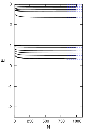
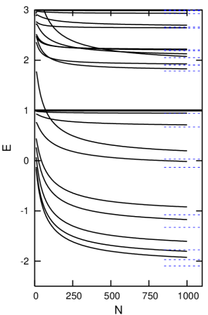
Figure 1: The dependence of the approximate eigenvalues on the number of point potentials for $B=1$, $R=2$ and $\gamma=1$ (a) and $\gamma=3$ (b). The dashed lines represent the exact eigenvalues of $H_{\gamma m}$.

Figure 1 depicts the comparison of the approximate and exact eigenvalues in two lowest gaps for two situations which differ only in the coupling constant $\gamma$. Figure 1 corresponds to a stronger attractive potential $\gamma=3$, therefore the eigenvalues are further from the Landau levels than those in 1 where $\gamma=1$. We observe that the approximate eigenvalues tend to the exact ones as the number of point potentials grows and that the convergence is slower when the coupling is stronger. One can roughly estimate that the convergence rate is of the type $cN^{-a}$, where according to numerical calculations, $a$ appears to be around $1/2$, while coefficient $c$ depends strongly on the coupling constant $\gamma$.

A close inspection of the eigenfunctions of the point potential operators would reveal that they have logarithmic peaks at the potential sites, since they are given as linear combinations of free Green functions, see e.g. [AGHH, chapter II]. Although by [Po2, theorem 3.4], these wavefunctions yield an approximation of wavefunctions of $H_{\gamma m}$, the peaks are of course absent in exact eigenfunctions. We believe that this fact is partly responsible for the slow convergence of the approximate energies of the bound states to the exact ones.

All the features we have described were observed in the non-magnetic case, see [EN2], with the exception that there one deals only with one gap $(-\infty,0)$ and the number of eigenvalues in the gap is finite. In the absence of magnetic field the ground state of $H_{\gamma m}$ corresponds to angular momentum $l=0$, the remaining bound states correspond to $\pm l$ and they are double degenerate. In magnetic field there is no such degeneracy; eigenvalues for angular momenta with opposite signs are different, because there is an extra angular momentum coming from the magnetic field. As figure 1 suggests, also the approximate eigenvalues (and in particular, their dependence on the number of point potentials) behave differently: the eigenvalue crossing the Landau level $B=1$ tends to the eigenvalue of $H_{\gamma m}$ for $l=1$, while the eigenvalue for $l=-1$ is the limit point of the second lowest approximate eigenvalue.

Acknowledgement

The research is supported by the Marie Curie grant MEIF-CT-2004-009256. The author thanks P. Exner for his constant support throughout the work and J. F. Brasche for many helpful suggestions.

References

• [AS] M.S. Abramowitz, I.A. Stegun (ed): Handbook of Mathematical Functions, Dover, New York 1965.
• [AGHH] S. Albeverio, F. Gesztesy, R. Høegh-Krohn, H. Holden: Solvable Models in Quantum Mechanics, Springer, Heidelberg 1988.
• [AHS] J. Avron, I. Herbst, B. Simon: Schrödinger operators with magnetic fields. I. General interactions, Duke Math. J. 45 (1978), 847–883.
• [B] J.F. Brasche: Upper bounds for Neumann-Schatten norms, Potential Anal. 14 (2001), 175–205.
• [BEKŠ] J.F. Brasche, P. Exner, Y.A. Kuperin, P. Šeba: Schrödinger operators with singular interactions, J. Math. Anal. Appl. 184 (1994), 112–139.
• [BFT] J. F. Brasche, R. Figari, A. Teta: Singular Schrödinger operators with singular interactions, Potential Anal. 8 (1998), 163–178.
• [BGP1] J. Brüning, V. Geyler, K. Pankrashkin: Continuity of integral kernels related to Schrödinger operators on manifolds, preprint math-ph/0410042
• [BGP2] J. Brüning, V. Geyler, K. Pankrashkin: On-diagonal singularities of the Green functions for Schrödinger operators, J. Math. Phys. 46 (2005), 113508–23.
• [CFKS] H.L. Cycon, R.G. Froese, W. Kirsch, B. Simon: Schrödinger operators, Springer, Berlin 1987.
• [DMM] V.V. Dodonov, I.A.Malkin, V.I. Man’ko: The Green function of the stationary Schrödinger equation for a particle in a uniform magnetic field, Phys. Lett. A51 (1975), 133–134.
• [EN1] P. Exner, K. Němcová: Finite number of point interactions in a layer, J. Math. Phys. 43 (2002), 1152–1184.
• [EN2] P. Exner, K. Němcová: Leaky quantum graphs: approximations by point interaction Hamiltonians, J. Phys. A36 (2003), 10173–10193.
• [ET] P. Exner, M. Tater: Spectra of soft ring graphs, Waves in Random Media 14 (2004), S47–60.
• [GHS] F. Gesztesy, H. Holden, P. Šeba: On point interactions in magnetic field system, in Schrödinger Operators, Standard and Non-standard (P. Exner, P. Šeba, eds.), World Scientific, Singapore 1989, 147–164.
• [GMC] V.A. Geyler, V.A.Margulis, I.I. Chuchaev: Zero-range potentials and Carleman operators, Sibirskij Math. J. 30 (1995), 828–841.
• [HSU] H. Hess, R. Schrader, D. A. Uhlenbrock: Domination of semigroups and generalization of Kato’s inequality, Duke Math. J. 44 (1977), 893–904.
• [KS] V. Kostrykin, R. Schrader: Kirchhoff’s rule for quantum wires, J. Phys. A32 (1999), 595–630.
• [K] P. Kuchment: Quantum graphs I. Some basic structures, Waves in Random media 14 (2004), S107–S128.
• [Po1] A. Posilicano: A Krein-like formula for singular perturbations of self-adjoint operators and applications, J. Funct. Anal. 183 (2001), 109–147.
• [Po2] A. Posilicano: Boundary triples and Weyl functions for singular perturbations of self-adjoint operators, Funct. Anal. Topol. 10 (2004), 57–63.
• [RS] M. Reed and B. Simon: Methods of Modern Mathematical Physics, Academic Press, New York 1975–1979.
• [SV] P. Stollmann, J. Voigt: Perturbation of Dirichlet forms by measures, Potential Anal. 5 (1996), 109–138.