CONVERGENCE OF SCHRÖDINGER OPERATORS

a) Institute of Mathematics, TU Clausthal, 38678 Clausthal-Z., Germany
b) Department of Mathematics, CTH $\&$ GU, 41296 Göteborg, Sweden
a) brasche@math.chalmers.se, nemco@math.chalmers.se

Abstract: We prove two limit relations between Schrödinger operators perturbed by measures. First, weak convergence of finite real-valued Radon measures $\mu_{n}\longrightarrow m$ implies that the operators $-{\Delta}+{\varepsilon}^{2}{\Delta}^{2}+\mu_{n}$ in $L^{2}({\mathbb{R}}^{d},dx)$ converge to $-{\Delta}+{\varepsilon}^{2}{\Delta}^{2}+m$ in the norm resolvent sense, provided $d\leq 3$. Second, for a large family, including the Kato class, of real-valued Radon measures $m$, the operators $-{\Delta}+{\varepsilon}^{2}{\Delta}^{2}+m$ tend to the operator $-{\Delta}+m$ in the norm resolvent sense as ${\varepsilon}$ tends to zero. Explicit upper bounds for the rates of convergences are derived. Since one can choose point measures $\mu_{n}$ with mass at only finitely many points, a combination of both convergence results leads to an efficient method for the numerical computation of the eigenvalues in the discrete spectrum and corresponding eigenfunctions of Schrödinger operators. The approximation is illustrated by numerical calculations of eigenvalues for one simple example of measure $m$.

I Introduction

In this paper we are going to analyze convergence of Schrödinger operators perturbed by measures. It is known that weak convergence of potentials implies norm-resolvent convergence of the corresponding one-dimensional Schrödinger operators. This result from [6] may be interesting for several reasons. For instance every finite real-valued Radon measure on ${\mathbb{R}}$ is the weak limit of a sequence of point measures with mass at only finitely many points. There exist efficient numerical methods for the computation of the eigenvalues and corresponding eigenfunctions of one-dimensional Schrödinger operators with a potential supported by a finite set; actually the effort for the computation grows at most linearly with the number of points of the support [9]. Since the norm resolvent convergence implies convergence of the eigenvalues in the discrete spectra and corresponding eigenspaces, we get an efficient method for the numerical calculation of the discrete spectra of one-dimensional Schrödinger operators. Norm resolvent convergence has also other important consequences: locally uniform convergence of the associated unitary groups and semigroups, convergence of the spectral projectors (which implies the mentioned results on the discrete spectra) etc.

Let us also mention a completely different motivation for studying convergence of operators with point potentials. In quantum mechanics neutron scattering is often described via so called zero-range Hamiltonians (the monograph [1] is an excellent standard reference to this research area). In a wide variety of models the positions of the neutrons are described via a family $(X_{j})_{j=1}^{n}$ of independent random variables with joint distribution $\mu$. Usually the number $n$ of neutrons is large and one is interested in the limit when $n$ tends to infinity and the strengths of the single size potentials tend to zero. In the one-dimensional case this motivates to investigate the limits of operators of the form

$$-\frac{d^{2}}{dx^{2}}+\frac{a}{n}\sum_{j=1}^{n}\delta_{X_{j}({\omega})},\qquad{\omega}\in{\Omega},$$

$a\not=0$ being a real constant and $({\Omega},{\cal F},{\mathbb{P}})$ a probability space. By the theorem of Glivenko-Cantelli, for ${\mathbb{P}}$-almost all ${\omega}\in{\Omega}$ the sequence $(\frac{a}{n}\sum_{j=1}^{n}\delta_{X_{j}({\omega})})_{n\in{\mathbb{N}}}$ converges to the measure $a\mu$ weakly. By the mentioned result from [6], this implies that

$$-\frac{d^{2}}{dx^{2}}+a\mu=\lim_{n\longrightarrow\infty}\left(-\frac{d^{2}}{dx^{2}}+\frac{a}{n}\sum_{j=1}^{n}\delta_{X_{j}({\omega})}\right)$$

in the norm resolvent sense ${\mathbb{P}}$-a.s.

It is the purpose of the present note to derive analogous results in the two- and three-dimensional case. It was shown in [6] and [8] that one can approximate Schrödinger operators perturbed by suitable measures by point potential Hamiltonian. However, the convergence there was in the strong resolvent sense, which is of course a weaker result than the norm resolvent convergence.

If the dimension is higher than one, then it seems to be impossible to work directly with operators of the form $-{\Delta}+\mu$, $\mu$ being a point measure. In fact, while the operators $-\frac{d^{2}}{dx^{2}}+\sum_{j=1}^{n}a_{j}\delta_{x_{j}}$ can be defined in dimension one via Kato’s quadratic form method as the unique lower semibounded self-adjoint operator associated to the energy form

$$D({\cal E}) := H^{1}({\mathbb{R}}),$$

$${\cal E}(f,f) := \int|f^{\prime}(x)|^{2}dx+\sum_{j=1}^{n}a_{j}|\tilde{f}(x_{j})|^{2},\quad f\in D({\cal E}),$$

$\tilde{f}$ being the unique continuous representative of $f\in H^{1}({\mathbb{R}})$, in higher dimension $d>1$, the quadratic form

$$D({\cal E}) := \{f\in H^{1}({\mathbb{R}}^{d}):f\mbox{ has a continuous representative }\tilde{f}\},$$

$${\cal E}(f,f) := \int|\nabla f(x)|^{2}dx+\sum_{j=1}^{n}a_{j}|\tilde{f}(x_{j})|^{2},\quad f\in D({\cal E}),$$

is not lower semibounded and closable if at least one coefficient $a_{j}$ is different from zero.

The strategy to overcome the mentioned problem in higher dimensions is based on two simple observations:

1. The lower semibounded self-adjoint operator ${\Delta}^{2}+\mu$ can be defined via Kato’s quadratic form method for every real-valued finite Radon measure $\mu$ on ${\mathbb{R}}^{d}$ (if $d\in\{1,2,3\}$), including point measures.

2. $-{\Delta}+{\varepsilon}^{2}{\Delta}^{2}\longrightarrow-{\Delta}$ in the norm resolvent sense, as ${\varepsilon}>0$ tends to zero.

We show the convergence claim in two steps. In section II we shall prove that the sequence $(-{\Delta}+{\varepsilon}^{2}{\Delta}^{2}+\mu_{n})_{n\in{\mathbb{N}}}$ converges to $-{\Delta}+{\varepsilon}^{2}{\Delta}^{2}+m$ in the norm resolvent sense provided $d\leq 3$, ${\varepsilon}>0$ and the finite real-valued Radon measures $\mu_{n}$ on ${\mathbb{R}}^{d}$ converge to the finite real-valued Radon measure $m$ weakly. Then, for a large class of measures $m$ we shall prove that

$$-{\Delta}+{\varepsilon}^{2}{\Delta}^{2}+m\longrightarrow-{\Delta}+m$$

in the norm resolvent sense as ${\varepsilon}$ tends to zero, cf. section III. Actually, we will not only prove convergence but also give explicit error estimates.

As approximating measures $\mu_{n}$ we can, in particular, choose point measures with mass at only finitely many points. In section IV we will present formulae which make it possible to calculate the eigenvalues and corresponding eigenspaces of operators perturbed by a finite number point measures. Then similarly to [1, chapter II.2], the spectral problem means to solve an implicit equation and the effort for these computations grows at most as ${\cal O}(n^{3})$.

Putting both convergence results from sections II and III and formulae from section IV together, we get an efficient method to calculate the eigenvalues in the discrete spectrum and corresponding eigenspaces of Schrödinger operators $-{\Delta}+m$ numerically. We apply the approximation to the simple two-dimensional example, where measure $m$ is negative and supported by a circle.

Our method does not only cover the case when $m$ is absolutely continuous w.r.t. the $(d-1)$-dimensional volume measure of a manifold with codimension one but a fairly large class of measures $m$ containing the set of all finite real-valued measures belonging to the Kato class. In particular, the absolutely continuous case $dm=Vdx$ where $-{\Delta}+m=-{\Delta}+V$ is a regular Schrödinger operator is contained in our approach. We refer to [10] for related convergence results in the regular case.

Notation and auxiliary results: Let $\mu$ be a real-valued Radon measure on ${\mathbb{R}}^{d}$. By the Hahn-Jordan theorem, there exist unique positive Radon measures $\mu^{\pm}$ on ${\mathbb{R}}^{d}$ such that

$$\mu=\mu^{+}-\mu^{-}\mbox{ and }\mu^{+}({\mathbb{R}}^{d}\setminus B)=0=\mu^{-}(B)$$

for some suitably chosen Borel set $B$. We put

$$\parallel\mu\parallel:=\mu^{+}({\mathbb{R}}^{d})+\mu^{-}({\mathbb{R}}^{d})\mbox{ and }|\mu|:=\mu^{+}+\mu^{-}.$$

If $\mu$ is finite, then we define its Fourier transform $\hat{\mu}$ as

$$\hat{\mu}(p):=(2\pi)^{-d/2}\int e^{ipx}\mu(dx),\qquad p\in{\mathbb{R}}^{d}.$$

Similarly, $\hat{f}$ also denotes the Fourier transform of $f\in L^{2}(dx):=L^{2}({\mathbb{R}}^{d},dx)$, $dx$ being the Lebesgue measure.

For $s>0$ we denote the Sobolev space of order $s$ by $H^{s}({\mathbb{R}}^{d})$, i.e.

$$H^{s}({\mathbb{R}}^{d}) := \left\{f\in L^{2}(dx):\,\int(1+p^{2})^{s}|\hat{f}(p)|^{2}dp<\infty\right\},$$

$$\parallel f\parallel_{H^{s}} := \left(\int(1+p^{2})^{s}|\hat{f}(p)|^{2}dp\right)^{1/2},\qquad f\in H^{s}({\mathbb{R}}^{d}).$$

We shall use occasionally the abbreviations $L^{2}(\mu):=L^{2}({\mathbb{R}}^{d},\mu)$ and $H^{s}:=H^{s}({\mathbb{R}}^{d})$.

$\parallel T\parallel_{{\cal H}_{1},{\cal H}_{2}}$ denotes the operator norm of $T$ as an operator from ${\cal H}_{1}$ to ${\cal H}_{2}$ and
$\parallel T\parallel_{{\cal H}}:=\parallel T\parallel_{{\cal H},{\cal H}}$. $\parallel f\parallel_{{\cal H}}$ and $(f,h)_{{\cal H}}$ represent the norm and the scalar product in the Hilbert ${\cal H}$, respectively. If the reference to a measure is missing, then we tacitly refer to the Lebesgue measure $dx$. For instance “integrable” means “integrable w.r.t. $dx$” if not stated otherwise, $\parallel T\parallel$, $(f,h)$ and $\parallel f\parallel$ denote the operator norm of $T$, scalar product and norm in the Hilbert space $L^{2}(dx)$, respectively. We denote by $C_{0}^{\infty}({\mathbb{R}}^{d})$ the space of smooth functions with compact support.

For arbitrary ${\varepsilon}\geq 0$ (${\varepsilon}=0$ will be admitted only in section III) let ${\cal E}_{{\varepsilon}}$ be the nonnegative closed quadratic form in the Hilbert space $L^{2}(dx)$ associated to the nonnegative self-adjoint operator $-{\Delta}+{\varepsilon}^{2}{\Delta}^{2}$ in $L^{2}(dx)$. Obviously we have

$$D({\cal E}_{{\varepsilon}}) = H^{2}({\mathbb{R}}^{d}),$$

$${\cal E}_{{\varepsilon}}(f,f) = {\varepsilon}^{2}\,({\Delta}f,{\Delta}f)+(\nabla f,\nabla f)\geq{\varepsilon}^{2}\,({\Delta}f,{\Delta}f),\qquad f\in D({\cal E}_{{\varepsilon}}),$$

for every ${\varepsilon}>0$. Note that for ${\varepsilon}=0$ the form domain is $H^{1}({\mathbb{R}}^{d})$ and ${\cal E}_{0}$ is the classical Dirichlet form. For any $\alpha>0$ we put

$${\cal E}_{{\varepsilon},\alpha}(f,h):={\cal E}_{{\varepsilon}}(f,h)+\alpha(f,h),\qquad f,h\in D({\cal E}_{{\varepsilon}}).$$

II Operator norm convergence

Throughout this section let $d\leq 3$ and $\mu$ be a finite real-valued Radon measure on ${\mathbb{R}}^{d}$. Then, by Sobolev’s embedding theorem, for every $s>3/2$, and, in particular, for $s=2$, every $f\in H^{s}({\mathbb{R}}^{d})$ has a unique continuous representative $\tilde{f}$ and

$$\parallel\tilde{f}\parallel_{\infty}:=\sup\{|\tilde{f}(x)|:\,x\in{\mathbb{R}}^{d}\}\leq c_{s}\parallel f\parallel_{H^{s}},\qquad f\in H^{s}({\mathbb{R}}^{d}),$$ (1)

for some finite constant $c_{s}$. Note that $c_{s}\leq 1$ if $s=2$. It follows that for every ${\varepsilon}>0$ and every $\eta>0$ there exists an $\alpha=\alpha({\varepsilon},\eta)<\infty$ such that

$$\parallel\tilde{f}\parallel_{\infty}^{2}\leq\eta\,{\cal E}_{{\varepsilon}}(f,f)+\alpha(f,f),\qquad f\in H^{2}({\mathbb{R}}^{d}).$$ (2)

Since $\mu$ is finite, for arbitrary ${\varepsilon},\eta>0$ and some finite $\alpha$ we get

$$|\int|\tilde{f}|^{2}d\mu|\leq\eta\parallel\mu\parallel{\cal E}_{{\varepsilon}}(f,f)+\alpha\parallel\mu\parallel(f,f),\qquad f\in H^{2}({\mathbb{R}}^{d}).$$ (3)

We put

$$D({\cal E}_{{\varepsilon}}^{\mu}) := H^{2}({\mathbb{R}}^{d}),$$

$${\cal E}_{{\varepsilon}}^{\mu}(f,f) := {\cal E}_{{\varepsilon}}(f,f)+\int|\tilde{f}|^{2}d\mu,\qquad f\in D({\cal E}_{{\varepsilon}}^{\mu}).$$

By (3) and the KLMN-theorem, ${\cal E}_{{\varepsilon}}^{\mu}$ is a lower semibounded closed quadratic form in $L^{2}(dx)$. We denote the lower semibounded self-adjoint operator in $L^{2}(dx)$ associated to ${\cal E}_{{\varepsilon}}^{\mu}$ by $-{\Delta}+{\varepsilon}^{2}{\Delta}^{2}+\mu$.

Our main tool to prove convergence results will be a Krein-like formula which expresses the resolvent $(-{\Delta}+{\varepsilon}^{2}{\Delta}^{2}+\mu+\alpha)^{-1}$ by means of the resolvent

$$G_{{\varepsilon},\alpha}:=(-{\Delta}+{\varepsilon}^{2}{\Delta}^{2}+\alpha)^{-1}.$$

The operator $G_{{\varepsilon},\alpha}$ has the integral kernel $g_{{\varepsilon},\alpha}(x-y)$ with Fourier transform

$$\hat{g}_{{\varepsilon},\alpha}(p):=\frac{1}{{\varepsilon}^{2}p^{4}+p^{2}+\alpha},\qquad p\in{\mathbb{R}}^{d}.$$

For every ${\varepsilon}\geq 0$ and $\alpha>0$, the function $g_{{\varepsilon},\alpha}(x)$ is continuous on ${\mathbb{R}}^{d}\setminus\{0\}$ and if $d=1$ or if $d\leq 3$ and ${\varepsilon}>0$ it is continuous on whole ${\mathbb{R}}^{d}$. Moreover, it is radially symmetric. Finally, $g_{0,\alpha}$ is the Green function of the free Laplacian in ${\mathbb{R}}^{d}$ and it is nonnegative. By the dominated convergence theorem,

$$\parallel g_{{\varepsilon},\alpha}\parallel_{H^{2}}^{2}=\int\frac{(1+p^{2})^{2}}{|{\varepsilon}^{2}p^{4}+p^{2}+\alpha|^{2}}\,dp\longrightarrow 0,\qquad\mbox{as }|\alpha|\longrightarrow\infty$$ (4)

which, by Sobolev’s inequality, implies that

$$\parallel g_{{\varepsilon},\alpha}\parallel_{\infty}\longrightarrow 0,\qquad\mbox{as }|\alpha|\longrightarrow\infty.$$ (5)

The fact that $g_{{\varepsilon},\alpha}$ is the Green function of $-{\Delta}+{\varepsilon}^{2}{\Delta}^{2}$ means that

$$\int g_{{\varepsilon},\alpha}(x-y)(-{\Delta}+{\varepsilon}^{2}{\Delta}^{2}+\alpha)h(y)dy=h(x)\qquad dx\mbox{-a.e.}$$

for all $h\in D(-{\Delta}+{\varepsilon}^{2}{\Delta}^{2})=H^{4}({\mathbb{R}}^{d})$. The equation above does not only hold almost everywhere w.r.t. the Lebesgue measure $dx$ but even pointwise everywhere, as the following lemma states.

              LEMMA 1

Let Green function $g_{{\varepsilon},\alpha}$ and operator $-{\Delta}+{\varepsilon}^{2}{\Delta}^{2}+\alpha$ be defined as above. Then one has

$$\int g_{{\varepsilon},\alpha}(x-y)(-{\Delta}+{\varepsilon}^{2}{\Delta}^{2}+\alpha)h(y)dy=\tilde{h}(x),\qquad x\in{\mathbb{R}}^{d}$$ (6)

for all $h\in H^{4}({\mathbb{R}}^{d})$.

Proof: In fact, we have only to show that the integral on the left hand side is a continuous function of $x\in{\mathbb{R}}^{d}$. We choose any sequence $(f_{n})_{n\in{\mathbb{N}}}$ of continuous functions with compact support converging to $(-{\Delta}+{\varepsilon}^{2}{\Delta}^{2}+\alpha)h$ in $L^{2}(dx)$. By (4), $g_{{\varepsilon},\alpha}\in H^{2}({\mathbb{R}}^{d})\subset L^{2}(dx)$, therefore we can write

$$\int g_{{\varepsilon},\alpha}(x-y)(-{\Delta}+{\varepsilon}^{2}{\Delta}^{2}+\alpha)h(y)dy=\lim_{n\longrightarrow\infty}\int g_{{\varepsilon},\alpha}(x-y)f_{n}(y)dy,\qquad x\in{\mathbb{R}}^{d}.$$

Obviously the mapping $x\mapsto\int g_{{\varepsilon},\alpha}(x-y)f_{n}(y)dy$, ${\mathbb{R}}^{d}\longrightarrow{\mathbb{C}}$, is the unique continuous representative $\widetilde{G_{{\varepsilon},\alpha}f_{n}}$ of $G_{{\varepsilon},\alpha}f_{n}$ for every $n\in{\mathbb{N}}$. Since $G_{{\varepsilon},\alpha}$ is a bounded operator from $L^{2}(dx)$ to $H^{2}({\mathbb{R}}^{d})$ (even to $H^{4}({\mathbb{R}}^{d})$), the sequence $(G_{{\varepsilon},\alpha}f_{n})_{n\in{\mathbb{N}}}$ converges in $H^{2}({\mathbb{R}}^{d})$ to $G_{{\varepsilon},\alpha}(-{\Delta}+{\varepsilon}^{2}{\Delta}^{2}+\alpha)h=h$. By Sobolev’s inequality (1), this implies that the sequence $(\widetilde{G_{{\varepsilon},\alpha}f_{n}})_{n\in{\mathbb{N}}}$ of the unique continuous representatives converges to a continuous function uniformly. By the last equality, $x\mapsto\int g_{{\varepsilon},\alpha}(x-y)(-{\Delta}+{\varepsilon}^{2}{\Delta}^{2}+\alpha)h(y)dy$, ${\mathbb{R}}^{d}\longrightarrow{\mathbb{C}}$, is this continuous uniform limit and we have proved (6). $\Box$

We introduce following integral operator

$$G_{{\varepsilon},\alpha}^{\mu}f(x):=\int g_{{\varepsilon},\alpha}(x-y)\tilde{f}(y)\mu(dy)\qquad dx\mbox{-a.e., }f\in H^{2}({\mathbb{R}}^{d}).$$

We can prove several estimates of its operator norm.

              LEMMA 2

The operator $G_{{\varepsilon},\alpha}^{\mu}$ is bounded on $H^{2}({\mathbb{R}}^{d})$ and its operator norm $\parallel G^{\mu}_{{\varepsilon},\alpha}\parallel_{H^{2}}$ decays with $\alpha\longrightarrow\infty$. The operator is bounded also w.r.t. other operator norms, in particular there are finite real numbers $c_{i}$, $i=1,2,3$ such that

$$\parallel G_{{\varepsilon},\alpha}^{\mu}f\parallel_{H^{2}} \leq c_{1}(\alpha)\parallel\tilde{f}\parallel_{\infty}$$

$$\parallel G_{{\varepsilon},\alpha}^{\mu}f\parallel_{L^{2}} \leq c_{2}(\alpha)\parallel\tilde{f}\parallel_{L^{2}(|\mu|)}\qquad f\in H^{2}({\mathbb{R}}^{d})$$

$$\parallel\widetilde{G_{{\varepsilon},\alpha}^{\mu}f}\parallel_{L^{2}(|\mu|)} \leq c_{3}(\alpha)\parallel\tilde{f}\parallel_{L^{2}(|\mu|)}$$

and all three numbers $c_{i}$ vanish in the limit $\alpha\longrightarrow\infty$.

Proof: Using Sobolev’s inequality we have for arbitrary $f\in H^{2}({\mathbb{R}}^{d})$

$$|\widehat{\tilde{f}\mu}(p)|^{2}\leq(2\pi)^{-d}\parallel\tilde{f}\parallel_{\infty}^{2}\parallel\mu\parallel^{2}\leq(2\pi)^{-d}\parallel\tilde{f}\parallel_{H^{2}}^{2}\parallel\mu\parallel^{2},\qquad p\in{\mathbb{R}}^{d}.$$

Then the convolution theorem yields

$$\parallel G_{{\varepsilon},\alpha}^{\mu}f\parallel_{H^{2}}^{2} = \int|(1+p^{2})^{2}|\,|({g_{{\varepsilon},\alpha}*\tilde{f}\mu}\hat{)}(p)|^{2}dp$$

$$= (2\pi)^{d}\int\frac{(1+p^{2})^{2}}{|{\varepsilon}^{2}p^{4}+p^{2}+\alpha|^{2}}\,|\widehat{\tilde{f}\mu}(p)|^{2}dp$$

$$\leq \int\frac{(1+p^{2})^{2}}{|{\varepsilon}^{2}p^{4}+p^{2}+\alpha|^{2}}\,\parallel\tilde{f}\parallel_{\infty}^{2}\parallel\mu\parallel^{2}dp$$

$$\leq \int\frac{(1+p^{2})^{2}}{|{\varepsilon}^{2}p^{4}+p^{2}+\alpha|^{2}}\,dp\,\parallel\tilde{f}\parallel_{H^{2}}^{2}\parallel\mu\parallel^{2}<\infty,\qquad f\in H^{2}({\mathbb{R}}^{d}).$$

Therefore $G_{{\varepsilon},\alpha}^{\mu}$ is an everywhere defined bounded operator on $H^{2}({\mathbb{R}}^{d})$ and we get an upper bound for the norm

$$\parallel G_{{\varepsilon},\alpha}^{\mu}\parallel_{H^{2},H^{2}}\leq\parallel\mu\parallel\left(\int\frac{(1+p^{2})^{2}}{|{\varepsilon}^{2}p^{4}+p^{2}+\alpha|^{2}}dp\right)^{1/2},$$ (7)

and the expression on the r.h.s. is also the uniform upper bound $c_{1}$.

To determine the remaining upper bounds $c_{2}$ and $c_{3}$, we can write

$$\int|G_{{\varepsilon},\alpha}^{\mu}f(x)|^{2}dx$$

$$= \int|\int g_{{\varepsilon},\alpha}(x-y)\tilde{f}(y)\mu^{+}(dy)-\int g_{{\varepsilon},\alpha}(x-y)\tilde{f}(y)\mu^{-}(dy)|^{2}dx$$

$$\leq 2\int|\int g_{{\varepsilon},\alpha}(x-y)\tilde{f}(y)\mu^{+}(dy)|^{2}dx+2\int|\int g_{{\varepsilon},\alpha}(x-y)\tilde{f}(y)\mu^{-}(dy)|^{2}dx$$

$$\leq 2\int\int|g_{{\varepsilon},\alpha}(x-y)|^{2}\mu^{+}(dy)\,\int|\tilde{f}(y)|^{2}\mu^{+}(dy)\,dx$$

$$+ 2\int\int|g_{{\varepsilon},\alpha}(x-y)|^{2}\mu^{-}(dy)\,\int|\tilde{f}(y)|^{2}\mu^{-}(dy)\,dx$$

$$\leq 2\int|g_{{\varepsilon},\alpha}(x)|^{2}dx\,\parallel\mu\parallel\,\int|\tilde{f}(y)|^{2}|\mu|(dy),\qquad f\in H^{2}({\mathbb{R}}^{d}).$$ (8)

In a similar way we arrive at

$$\int|\widetilde{G_{{\varepsilon},\alpha}^{\mu}f}(x)|^{2}|\mu|(dx)\leq 2\parallel g_{{\varepsilon},\alpha}\parallel_{\infty}^{2}\parallel\mu\parallel^{2}\int|\tilde{f}(y)|^{2}|\mu|(dy).$$

Finally, from (4) and (5) one concludes that all the upper bounds of the operator norms tend to zero in the limit $\alpha\longrightarrow\infty$. $\Box$

General results of [3] (cf. also section III below) provide, in particular, an explicit formula for the resolvent of the operator $-{\Delta}+{\varepsilon}^{2}{\Delta}^{2}+\mu$. In this resolvent formula there occur operators acting in different Hilbert spaces. This is inconvenient when we investigate the convergence of sequences of such operators and we shall use a slightly different resolvent formula:

$$(-{\Delta}+{\varepsilon}^{2}{\Delta}^{2}+\mu+\alpha)^{-1}=G_{{\varepsilon},\alpha}-G_{{\varepsilon},\alpha}^{\mu}(I+G_{{\varepsilon},\alpha}^{\mu})^{-1}G_{{\varepsilon},\alpha}.$$ (9)

For the sake of completeness we present the proof of the above Krein’s formula in the appendix. According to lemma 2, we can choose $\alpha>0$ such that $\parallel G_{{\varepsilon},\alpha}^{\mu}\parallel_{H^{2},H^{2}}<1$. Then the operator $I+G_{{\varepsilon},\alpha}^{\mu}$ is invertible and its inverse is everywhere defined on $H^{2}({\mathbb{R}}^{d})$ and bounded; here $I$ denotes the identity on $H^{2}({\mathbb{R}}^{d})$. By (3), we can choose $\alpha>0$ such that, in addition,

$${\cal E}_{{\varepsilon},\alpha}^{\mu}(f,f):={\cal E}_{{\varepsilon}}^{\mu}(f,f)+\alpha(f,f)\geq(f,f),\quad f\in D({\cal E}_{{\varepsilon}}^{\mu}).$$ (10)

We are now prepared for the proof of the main theorem of this section:

              THEOREM 3

Let $m$ and $\mu_{n}$, $n\in{\mathbb{N}}$, be finite real-valued Radon measures on ${\mathbb{R}}^{d}$. Suppose that the sequence $(\mu_{n})_{n\in{\mathbb{N}}}$ converges to $m$ weakly and $\sup_{n\in{\mathbb{N}}}\parallel\mu_{n}\parallel<\infty$. Let ${\varepsilon},\alpha>0$ and $d\in\{1,2,3\}$. Then the operators $-\Delta+{\varepsilon}^{2}\Delta^{2}+\mu_{n}$ converge to $-\Delta+{\varepsilon}^{2}\Delta^{2}+m$ in the norm resolvent sense.

Proof: Let ${\varepsilon}>0$ be arbitrary. We choose $0<c<1$ and $\alpha>0$ such that

$$\parallel\mu_{n}\parallel^{2}\int\frac{(1+p^{2})^{2}}{|{\varepsilon}^{2}p^{4}+p^{2}+\alpha|^{2}}\,dp\,\leq c^{2},\quad n\in{\mathbb{N}},$$ (11)

and

$$\parallel m\parallel^{2}\int\frac{(1+p^{2})^{2}}{|{\varepsilon}^{2}p^{4}+p^{2}+\alpha|^{2}}\,dp\,\leq c^{2}.$$ (12)

According to (3), we can choose $\alpha>0$ such that, in addition,

$${\cal E}_{{\varepsilon},\alpha}^{\mu_{n}}(f,f)\geq(f,f),\qquad f\in H^{2}({\mathbb{R}}^{d}),\quad n\in{\mathbb{N}}.$$ (13)

Since $(\mu_{n})_{n\in{\mathbb{N}}}$ converges to $m$ weakly, (13) also holds when we replace $\mu_{n}$ by $m$. By Lemma 2, in particular estimate (7), inequalities (11) and (12) yield

$$\parallel G_{{\varepsilon},\alpha}^{\mu_{n}}\parallel_{H^{2},H^{2}} \leq c,\qquad n\in{\mathbb{N}},$$

$$\parallel G_{{\varepsilon},\alpha}^{m}\parallel_{H^{2},H^{2}} \leq c,$$ (14)

$$\parallel G_{{\varepsilon},\alpha}^{m}f\parallel_{H^{2}} \leq c\parallel\tilde{f}\parallel_{\infty},\qquad f\in H^{2}({\mathbb{R}}^{d}).$$

Hence the resolvent formula (9) is valid both for $\mu=m$ and for $\mu=\mu_{n}$, $n\in{\mathbb{N}}$. By Lemma 2, we can choose $\alpha$ sufficiently large so that also

$$\int|G_{{\varepsilon},\alpha}^{m}h(x)|^{2}dx\leq c^{2}\int|\tilde{h}|^{2}d|m|\mbox{ and }\int|\widetilde{G_{{\varepsilon},\alpha}^{m}h}(x)|^{2}|m|(dx)\leq c^{2}\int|\tilde{h}|^{2}d|m|$$ (15)

for every $h\in H^{2}({\mathbb{R}}^{d})$.

For notational brevity we put

$$g_{0}:=g_{0,1},\quad g:=g_{{\varepsilon},\alpha},\quad G:=G_{{\varepsilon},\alpha},\quad G^{\mu_{n}}:=G_{{\varepsilon},\alpha}^{\mu_{n}}\quad\mbox{and}\quad G^{m}:=G_{{\varepsilon},\alpha}^{m}.$$

With this notation we have

$$(-{\Delta}+{\varepsilon}^{2}{\Delta}^{2}+\mu_{n}+\alpha)^{-1}-(-{\Delta}+{\varepsilon}^{2}{\Delta}^{2}+m+\alpha)^{-1}$$

$$= G^{m}[I+G^{m}]^{-1}G-G^{\mu_{n}}[I+G^{\mu_{n}}]^{-1}G$$

$$= (G^{m}-G^{\mu_{n}})[I+G^{m}]^{-1}G+(G^{\mu_{n}}-G^{m})[I+G^{m}]^{-1}(G^{\mu_{n}}-G^{m})[I+G^{\mu_{n}}]^{-1}G$$

$$+G^{m}[I+G^{m}]^{-1}(G^{\mu_{n}}-G^{m})[I+G^{\mu_{n}}]^{-1}G.$$

Since $G$ is a bounded operator from $L^{2}(dx)$ to $H^{2}({\mathbb{R}}^{d})$ we have only to show that

$$\parallel G^{m}-G^{\mu_{n}}\parallel_{H^{2},L^{2}(dx)}\longrightarrow 0\qquad\mbox{as }n\longrightarrow\infty,$$ (16)

$$\parallel G^{m}[I+G^{m}]^{-1}(G^{m}-G^{\mu_{n}})\parallel_{H^{2},L^{2}(dx)}\longrightarrow 0,\qquad\mbox{as }n\longrightarrow\infty.$$ (17)

We introduce

$$\nu_{n} := m-\mu_{n}$$

$$\nu_{nx}(dy) := g(x-y)\,\nu_{n}(dy),\qquad x\in{\mathbb{R}}^{d},\quad n\in{\mathbb{N}}.$$

As $d\leq 3$, the function

$$y\mapsto\int g_{0}(y-a)\,f(a)\,da$$

is continuous and bounded for every $f\in L^{2}(dx)$; this well known fact can be proved in the same way as (6). Since the function $g$ is bounded and $g_{0}$ is nonnegative it follows that

$$\left|\int|g(x-y)|\int|g_{0}(y-a)|\,|(-{\Delta}+1)h(a)|\,da\,\nu_{n}^{\pm}(dy)\right|<\infty$$

for all $x\in{\mathbb{R}}^{d}$ and $h\in H^{2}({\mathbb{R}}^{d})$. Hence by Fubini’s theorem, the function $k_{\nu_{nx}}:{\mathbb{R}}^{d}\longrightarrow{\mathbb{R}}$, defined by

$$k_{\nu_{nx}}(a):=\left\{\begin{array}[]{ll}\int g_{0}(y-a)\,g(x-y)\,\nu_{n}(dy),&\quad\mbox{if defined,}\\ 0,&\quad\mbox{otherwise,}\end{array}\right.$$ (20)

is Borel measurable, the integral on the right hand side is defined and finite for almost all $a\in{\mathbb{R}}^{d}$ (almost all w.r.t. the Lebesgue measure) and

$$|(G^{\nu_{n}}h\tilde{)}(x)|^{2} = |\int g(x-y)\,h(y)\,\nu_{n}(dy)|^{2}$$ (21)

$$= |\int g(x-y)\int g_{0}(y-a)(-{\Delta}+1)h(a)\,da\,\nu_{n}(dy)|^{2}$$

$$\leq \int|k_{\nu_{nx}}(a)|^{2}da\cdot\int|(-{\Delta}+1)h(a)|^{2}da$$

$$\leq 2\parallel h\parallel_{H^{2}}^{2}\int|k_{\nu_{nx}}(a)|^{2}da,\qquad h\in H^{2}({\mathbb{R}}^{d}),\,n\in{\mathbb{N}}.$$

Thus in order to prove (16) we have only to show that

$$\int\int|k_{\nu_{nx}}(a)|^{2}da\,dx\longrightarrow 0\qquad\mbox{as }n\longrightarrow\infty.$$ (22)

We have

$$\int\int|k_{\nu_{nx}}(a)|^{2}da\,dx=(2\pi)^{d}\int\int|\widehat{g_{0}}(p)|^{2}|\widehat{\nu_{nx}}(p)|^{2}dp\,dx$$

$$= \int\int\frac{1}{|1+p^{2}|^{2}}\int e^{ipy}g(x-y)\,\nu_{n}(dy)\int e^{-ipz}g(x-z)\nu_{n}(dz)\,dp\,dx.$$ (23)

Since $|1+p^{2}|^{-2}$ and $g$ are integrable w.r.t. the Lebesgue measure, $g$ is bounded and the Radon measures $\nu_{n}$ are finite, we can change the order of integration. Let us rewrite (II) as

$$\int f(y,z)\,h(y,z)\,\nu_{n}\otimes\nu_{n}(dy\,dz).$$

The function

$$f(y,z):=\int e^{ipy}e^{-ipz}\frac{1}{|1+p^{2}|^{2}}\,dp,\qquad y,z\in{\mathbb{R}}^{d},$$

is bounded and continuous. It follows from the fact that it is (up to multiplication by $(2\pi)^{d/2}$) the inverse Fourier transform of the integrable function $|1+p^{2}|^{-2}$ at the point $z-y$.

Also the function

$$h(y,z):=\int g(x-y)\,g(x-z)\,dx$$

is bounded and continuous for $y,z\in{\mathbb{R}}^{d}$. This can be shown using following observation. Let $y\in{\mathbb{R}}^{d}$ and $K$ be any compact neighborhood of $y$. Since $|x|^{j}g_{{\varepsilon},\alpha}(x)\longrightarrow 0$ for every $j\in N$ as $|x|\longrightarrow\infty$, there exists a constant $a<\infty$ such that

$$|g(x-y)\,g(x-z)|\leq a\parallel g\parallel_{\infty}\mbox{dist}(x,K)^{-4},\qquad x\in{\mathbb{R}}^{d}\setminus K,\quad z\in{\mathbb{R}}^{d},\quad y\in K.$$

By Stone-Weierstrass theorem, the set of functions of the form $\sum_{j=1}^{N}f_{j}(x)g_{j}(y)$, $N\in{\mathbb{N}}$, where $f_{j},g_{j}$ are bounded and continuous, is dense in the space of bounded continuous functions w.r.t. the supremum norm. Since the measures $\nu_{n}$ tend to zero weakly and $\sup_{n\in{\mathbb{N}}}\parallel\nu_{n}\parallel<\infty$, this implies that the product measures $\nu_{n}\otimes\nu_{n}$ tend to zero weakly, too. Hence by (II), we have proved (22) and therefore also (16).

It only remains to prove (17). For this purpose we first note that

$$c_{n}:=\int\int|k_{\nu_{nx}}(a)|^{2}\,da\,|m|(dx)\longrightarrow 0\qquad\mbox{as }n\longrightarrow\infty.$$

This can be shown by mimicking the proof of (22). By (21), it follows that

$$\int|(G^{\nu_{n}}h\tilde{)}(x)|^{2}\,|m|(dx)\leq 2c_{n}\parallel h\parallel_{H^{2}}^{2},\qquad h\in H^{2}({\mathbb{R}}^{d}).$$

Thus, in order to prove (17), we have only to show that there exists a finite constant $C$ such that

$$\parallel G^{m}(I+G^{m})^{-1}h\parallel_{L^{2}(dx)}\leq C\left(\int|\tilde{h}|^{2}d|m|\right)^{1/2},\qquad h\in H^{2}({\mathbb{R}}^{d}).$$ (24)

Using the estimates (II), we have

$$G^{m}(I+G^{m})^{-1}=-\sum_{j=1}^{\infty}(-G^{m})^{j}.$$ (25)

According to (15),

$$\parallel(G^{m})^{j+1}h\parallel_{L^{2}(dx)}\leq c\left(\int|\widetilde{(G^{m})^{j}h}|^{2}d|m|\right)^{1/2}\leq c\cdot c^{j}\left(\int|\tilde{h}|^{2}d|m|\right)^{1/2},$$

for every $j\in{\mathbb{N}}$ and hence

$$\parallel\sum_{j=1}^{\infty}(-G^{m})^{j}h\parallel_{L^{2}(dx)}\leq\sum_{j=1}^{\infty}c^{j}\left(\int|\tilde{h}|^{2}d|m|\right)^{1/2}=\frac{c}{1-c}\,\left(\int|\tilde{h}|^{2}d|m|\right)^{1/2}.$$

By (25), this implies (24) and the proof of the theorem is complete. $\Box$

              REMARK 4

We have shown that

$$\parallel(-{\Delta}+{\varepsilon}^{2}{\Delta}^{2}+\mu_{n}+\alpha)^{-1}-(-{\Delta}+{\varepsilon}^{2}{\Delta}^{2}+m+\alpha)^{-1}\parallel^{2}$$

$$\leq C_{1}\int\int|\int g_{0,1}(y-a)g_{{\varepsilon},\alpha}(x-y)(m-\mu_{n})(dy)|^{2}da\,dx$$

$$+C_{2}\int\int|\int g_{0,1}(y-a)g_{{\varepsilon},\alpha}(x-y)(m-\mu_{n})(dy)|^{2}da\,|m|(dx)$$

for some finite constants $C_{j}=C_{j}({\varepsilon},\alpha)$, $j=1,2$, which can be computed with the aid of the proof of theorem 3. Thus the proof provides explicit upper bounds for the error one makes when one replaces the operator $-{\Delta}+{\varepsilon}^{2}{\Delta}^{2}+m$ by $-{\Delta}+{\varepsilon}^{2}{\Delta}^{2}+\mu_{n}$.

              REMARK 5

The essential spectrum of $-{\Delta}+{\varepsilon}^{2}{\Delta}^{2}+m$ remains the same for any finite real-valued Radon measure $m$ on ${\mathbb{R}}^{d}$

$$\sigma_{ess}(-{\Delta}+{\varepsilon}^{2}{\Delta}^{2}+m)=\sigma_{ess}(-{\Delta}+{\varepsilon}^{2}{\Delta}^{2})=[0,\infty).$$

By Sobolev’s inequality and [4, Lemma 19], the mapping $f\mapsto\tilde{f}$ from $H^{2}({\mathbb{R}}^{d})$ to $L^{2}(|m|)$ is compact. Therefore using estimate (II), one may conclude that $G_{{\varepsilon},\alpha}^{\mu}$ is compact if regarded as an operator from $H^{2}({\mathbb{R}}^{d})$ to $L^{2}(dx)$. According to the resolvent formula (9), this implies that the resolvent difference $G_{{\varepsilon},\alpha}^{m}-G_{{\varepsilon},\alpha}$ is compact and hence the corresponding essential spectra coincide.

III Dependence on the coupling constant

In this section we are going to prove that

$$-{\Delta}+{\varepsilon}^{2}{\Delta}^{2}+m\longrightarrow-{\Delta}+m\qquad\mbox{as }{\varepsilon}\downarrow 0,$$ (26)

in the norm resolvent sense. Here $m$ denotes a real-valued Radon measure on ${\mathbb{R}}^{d}$ and we assume, in addition, that for every $\eta>0$ there exists a $\beta_{\eta}<\infty$ such that

$$\int|f|^{2}d|m|\leq\eta\left(\int|\nabla f|^{2}dx+\beta_{\eta}\int|f|^{2}dx\right),\qquad f\in C_{0}^{\infty}({\mathbb{R}}^{d}).$$ (27)

Note that we neither require that $m$ is finite nor that $d\leq 3$. On the other hand, the condition (27) implies that $m(B)=0$ for every Borel set $B$ with classical capacity zero and, for instance, it is excluded that $m$ is a point measure if $d>1$.

The inequality (27) holds, in particular, provided $m$ belongs to the Kato class, i.e.

$$\sup_{n\in{\mathbb{Z}}}|m|([n,n+1]) < \infty,\qquad d=1,$$

$$\lim_{\varepsilon\to 0}\sup_{x\in{\mathbb{R}}^{2}}\int_{B(x,\varepsilon)}|\log(|x-y|)|\,|m|(dy) = 0,\qquad d=2,$$

$$\lim_{\varepsilon\to 0}\sup_{x\in{\mathbb{R}}^{3}}\int_{B(x,\varepsilon)}\frac{1}{|x-y|}\,|m|(dy) = 0,\qquad d=3,$$

with $B(x,\varepsilon)$ denoting the ball of radius $\varepsilon$ centered at $x$ (cf. [11], Theorem 3.1). We refer to [7, chapter 1.2], for additional examples of measures satisfying (27).

In general, the elements $f$ in the form domain of $-{\Delta}$ do not possess a continuous representative $\tilde{f}$. Therefore we shall give a definition of ${\cal E}_{{\varepsilon}}^{m}$ different from the one in section II so that it works for all ${\varepsilon}\geq 0$. Of course, both definitions are equivalent in the special case of positive ${\varepsilon}$.

Since the space $C_{0}^{\infty}({\mathbb{R}}^{d})$ of smooth functions with compact support is dense in the Sobolev space $H^{1}({\mathbb{R}}^{d})$, there exists a unique bounded linear mapping $J_{m}:H^{1}({\mathbb{R}}^{d})\longrightarrow L^{2}(|m|)$ satisfying

$$J_{m}f=f,\qquad f\in C_{0}^{\infty}({\mathbb{R}}^{d}),$$

(strictly speaking $J_{m}$ maps the $dx$-equivalence class of the continuous function $\tilde{f}\in C_{0}^{\infty}({\mathbb{R}}^{d})$ to the $|m|$-equivalence class of $\tilde{f}$). We put

$$D({\cal E}_{{\varepsilon}}^{m}) := D({\cal E}_{{\varepsilon}}),$$

$${\cal E}_{{\varepsilon}}^{m}(f,f) := {\cal E}_{{\varepsilon}}(f,f)+(A_{m}J_{m}f,J_{m}f)_{L^{2}(|m|)},\qquad f\in D({\cal E}_{{\varepsilon}}^{m}),$$

where $D({\cal E}_{{\varepsilon}})=H^{1}({\mathbb{R}}^{d})$ for ${\varepsilon}=0$, $D({\cal E}_{{\varepsilon}})=H^{2}({\mathbb{R}}^{d})$ otherwise and

$$A_{m}h(x):=\left\{\begin{array}[]{ll}h(x),&\quad x\in B,\\ -h(x),&\quad x\in{\mathbb{R}}^{d}\setminus B,\end{array}\right.\qquad h\in L^{2}(|m|),$$

with $B$ being any Borel set such that $m^{+}({\mathbb{R}}^{d}\setminus B)=0=m^{-}(B)$. By (27) and the KLMN-theorem, the quadratic form ${\cal E}_{{\varepsilon}}^{m}$ in $L^{2}(dx)$ is lower semibounded and closed and

$${\cal E}_{{\varepsilon},\beta_{1}}^{m}(f,f)\geq 0,\qquad f\in D({\cal E}_{{\varepsilon}}^{m}).$$

Again, $-{\Delta}+{\varepsilon}^{2}{\Delta}^{2}+m$ denotes the lower semibounded self-adjoint operator associated to ${\cal E}_{{\varepsilon}}^{m}$ and we put

$$R_{{\varepsilon},\alpha}^{m}:=(-{\Delta}+{\varepsilon}^{2}{\Delta}^{2}+m+\alpha)^{-1}$$

provided the inverse operator exists. $G_{{\varepsilon},\alpha}$ is defined the same way as in section II.

One key for the proof of the convergence result (26) is the observation that one can decompose

$$\hat{g}_{{\varepsilon},\alpha}(p)=\frac{c({\varepsilon})}{p^{2}+\alpha({\varepsilon})}-\frac{c({\varepsilon})}{p^{2}+\beta({\varepsilon})},$$

whenever $c({\varepsilon})$ is defined. The coefficients $-\alpha({\varepsilon})$ and $-\beta({\varepsilon})$ are the roots of the polynomial ${\varepsilon}^{2}x^{2}+x+\alpha$; a simple calculation yields

$$c({\varepsilon}) := \frac{1}{\sqrt{1-4{\varepsilon}^{2}\alpha}}\qquad\longrightarrow 1,\qquad\mbox{as }{\varepsilon}\downarrow 0,$$

$$\alpha({\varepsilon}) := \frac{2\alpha}{1+\sqrt{1-4{\varepsilon}^{2}\alpha}}\longrightarrow\alpha,\qquad\mbox{as }{\varepsilon}\downarrow 0,$$ (29)

$$\beta({\varepsilon}) := \frac{1+\sqrt{1-4{\varepsilon}^{2}\alpha}}{2{\varepsilon}^{2}}\longrightarrow\infty,\qquad\mbox{as }{\varepsilon}\downarrow 0.$$

Using the parameters introduced above, we arrive at

$$G_{{\varepsilon},\alpha}=c({\varepsilon})G_{0,\alpha({\varepsilon})}-c({\varepsilon})G_{0,\beta({\varepsilon})}.$$ (30)

In the proof of the convergence result (26) we will use again a Krein-like resolvent formula, this time using the one from [3], cf.(32) below. First we need some preparation. Let $\alpha>0$ and ${\varepsilon}\geq 0$. We introduce the operator $J_{m,{\varepsilon},\alpha}$ from the Hilbert space $(D({\cal E}_{{\varepsilon}}),{\cal E}_{{\varepsilon},\alpha})$ to $L^{2}(|m|)$ as follows:

$$D(J_{m,{\varepsilon},\alpha}) := D({\cal E}_{{\varepsilon}}),$$

$$J_{m,{\varepsilon},\alpha}f := J_{m}f,\qquad f\in D(J_{m,{\varepsilon},\alpha}).$$

By (27), the operator norm of $J_{m,{\varepsilon},\alpha}$ is less than or equal to $\eta$ provided $\alpha\geq\beta_{\eta}$. Thus we can choose $\alpha_{0}>0$ and $c<1$ such that

$$\parallel J_{m,{\varepsilon},\alpha}\parallel_{(D({\cal E}_{{\varepsilon}}),{\cal E}_{{\varepsilon},\alpha}),L^{2}(|m|)}\,\leq\sqrt{c},\qquad\alpha\geq\alpha_{0}.$$ (31)

Due to (31), the hypothesis of Theorem 3 in [3] is satisfied and the theorem implies that $-\alpha$ belongs to the resolvent set of $-{\Delta}+{\varepsilon}^{2}{\Delta}^{2}+m$ and

$$R_{{\varepsilon},\alpha}^{m}=G_{{\varepsilon},\alpha}-(J_{m,{\varepsilon},\alpha})^{*}A_{m}(1+J_{m}J_{m,{\varepsilon},\alpha}^{*}A_{m})^{-1}J_{m}G_{{\varepsilon},\alpha},\qquad\alpha\geq\alpha_{0}.$$ (32)

In fact, we can write

$$J_{m,{\varepsilon},\alpha^{\prime}}^{*}=(J_{m}G_{{\varepsilon},\alpha^{\prime}})^{*},\qquad\alpha^{\prime}>0,$$ (33)

since we have

$$(J_{m,{\varepsilon},\alpha^{\prime}}^{*}f,h)={\cal E}_{{\varepsilon},\alpha^{\prime}}(J_{m,{\varepsilon},\alpha^{\prime}}^{*}f,G_{{\varepsilon},\alpha^{\prime}}h)=(f,J_{m,{\varepsilon},\alpha^{\prime}}G_{{\varepsilon},\alpha^{\prime}}h)_{L^{2}(|m|)}=((J_{m}G_{{\varepsilon},\alpha^{\prime}})^{*}f,h)$$

for every $h\in L^{2}(dx)$, ${\varepsilon}\geq 0$ and $\alpha^{\prime}>0$.

              THEOREM 6

Let $m$ be a real-valued Radon measure on ${\mathbb{R}}^{d}$ satisfying (27). Then the operators $-{\Delta}+{\varepsilon}^{2}{\Delta}^{2}+m$ converge to $-{\Delta}+m$ in the norm resolvent sense as ${\varepsilon}\downarrow 0$.

Proof: Both resolvents are written by means of Krein’s formula (32), so we can compare the first and second terms separately. To see that $\parallel G_{{\varepsilon},\alpha}-G_{0,\alpha}\parallel_{L^{2}(dx)}$ vanishes in the limit ${\varepsilon}\downarrow 0$ is simple. It is enough to use the first resolvent formula,

$$G_{0,\alpha({\varepsilon})}-G_{0,\alpha}=(\alpha-\alpha({\varepsilon}))G_{0,\alpha}G_{0,\alpha({\varepsilon})}$$ (34)

and the fact that

$$\parallel G_{0,\alpha^{\prime}}\parallel_{L^{2}(dx),H^{1}}^{2}\leq k(\alpha^{\prime}),\qquad\alpha^{\prime}>0,$$

for some continuous function $k$ vanishing at infinity (actually, $k(x)=1/x^{2}$ for $x\leq 2$ and $k(x)=1/(4(x-1))$ for $x>2$). Then the decomposition (30) of $G_{{\varepsilon},\alpha}$ and the asymptotic behavior (29) of $\alpha({\varepsilon}),\beta({\varepsilon})$ and $c({\varepsilon})$ finish the argument.

The proof that also the difference of second terms in Krein’s formula tend to zero as ${\varepsilon}\to 0$ can be reduced into two tasks

$$\parallel J_{m}G_{{\varepsilon},\alpha}-J_{m}G_{0,\alpha}\parallel_{L^{2}(dx),L^{2}(|m|)} \longrightarrow 0\qquad\mbox{as }{\varepsilon}\downarrow 0,$$

$$\parallel(1+J_{m}J_{m,{\varepsilon},\alpha}^{*}A_{m})^{-1}-(1+J_{m}J_{m,0,\alpha}^{*}A_{m})^{-1}\parallel_{L^{2}(|m|)} \longrightarrow 0\qquad\mbox{as }{\varepsilon}\downarrow 0.$$

The argument for the first line is similar to the one we have presented above for $G_{{\varepsilon},\alpha}-G_{0,\alpha}$, we only have to add that, by hypothesis (27), it follows that

$$\parallel J_{m}G_{0,\alpha^{\prime}}\parallel_{L^{2}(dx),L^{2}(|m|)}^{2}\leq\mbox{max}(1,\beta_{1})k(\alpha^{\prime}),\qquad\alpha^{\prime}>0,$$ (35)

where function $k(\alpha^{\prime})$ is defined as above.

To show the second line we choose any $\alpha>\alpha_{0}$, then from (31) we get

$$\parallel(1+J_{m}J_{m,{\varepsilon},\alpha}^{*}A_{m})^{-1}\parallel_{L^{2}(|m|)}\leq\frac{1}{1-c},\qquad{\varepsilon}\geq 0.$$

By the second resolvent identity

$$(1+A)^{-1}-(1+B)^{-1}=(1+A)^{-1}(B-A)(1+B)^{-1},$$

it is sufficient to prove that

$$\parallel J_{m}J_{m,{\varepsilon},\alpha}^{*}-J_{m}J_{m,0,\alpha}^{*}\parallel_{L^{2}(|m|)}\longrightarrow 0\qquad\mbox{as }{\varepsilon}\downarrow 0.$$ (36)

From (30) and (33) follows that

$$J_{m}J_{m,{\varepsilon},\alpha}^{*}=c({\varepsilon})J_{m}(J_{m}G_{0,\alpha({\varepsilon})})^{*}-c({\varepsilon})J_{m}(J_{m}G_{0,\beta({\varepsilon})})^{*},$$

note that $c({\varepsilon})$ is real for sufficiently small ${\varepsilon}$. Using this expression and (34) and (33), we get

$$\parallel J_{m}J_{m,{\varepsilon},\alpha}^{*}-J_{m}J_{m,0,\alpha}^{*}\parallel_{L^{2}(|m|)}$$

$$\leq \parallel(c({\varepsilon})-1)J_{m}(J_{m}G_{0,\alpha({\varepsilon})})^{*}\parallel_{L^{2}(|m|)}+\parallel J_{m}(J_{m}G_{0,\alpha({\varepsilon})})^{*}-J_{m}(J_{m}G_{0,\alpha})^{*}\parallel_{L^{2}(|m|)}$$

$$+\parallel c({\varepsilon})J_{m}(J_{m}G_{0,\beta({\varepsilon})})^{*}\parallel_{L^{2}(|m|)}$$

$$= \parallel(c({\varepsilon})-1)J_{m,0,\alpha({\varepsilon})}J_{m,0,\alpha({\varepsilon})}^{*}\parallel_{L^{2}(|m|)}+\parallel(\alpha-\alpha({\varepsilon}))J_{m}G_{0,\alpha}(J_{m}G_{0,\alpha({\varepsilon})})^{*}\parallel_{L^{2}(|m|)}$$

$$+\parallel c({\varepsilon})J_{m,0,\beta({\varepsilon})}J_{m,0,\beta({\varepsilon})}^{*}\parallel_{L^{2}(|m|)},\qquad{\varepsilon}>0.$$

According to (27), the mapping $\parallel J_{m,0,\alpha}J_{m,0,\alpha}^{*}\parallel_{L^{2}(|m|)}$ is locally bounded for $\alpha\in(0,\infty)$ and tends to zero as $\alpha$ tends to infinity. Since $\alpha({\varepsilon})\longrightarrow\alpha$, $c({\varepsilon})\longrightarrow 1$ and $\beta({\varepsilon})\longrightarrow\infty$ as ${\varepsilon}\downarrow 0$, this implies, in conjunction with (35), that (36) holds. $\Box$

              REMARK 7

By the proof above, $\parallel G_{{\varepsilon},\alpha}^{m}-G_{0,\alpha}^{m}\parallel$ is upper bounded by an expression of the form $c\cdot({\varepsilon}^{2}+\eta(m,{\varepsilon}))$ where the finite constant $c$ can be extracted from the proof and $\eta(m,{\varepsilon})$ has to be chosen (and can be chosen) such that (27) holds with $\eta$ and $\beta$ replaced by $\eta(m,{\varepsilon})$ and $\beta({\varepsilon})$, respectively.

IV Eigenvalues and eigenspaces of the approximating operators

Throughout this section let $d\leq 3$ and let $m$ be a finite real-valued Radon measure satisfying (27) (e.g., let $m$ be from the Kato class). By the two preceding convergence results, we can approximate the operator $-{\Delta}+m$ in $L^{2}({\mathbb{R}}^{d},dx)$ by operators of the form $-{\Delta}+{\varepsilon}^{2}{\Delta}^{2}+\mu$, where ${\varepsilon}>0$ and $\mu$ is a point measure with mass at only finitely many points. Since the convergence is in norm resolvent sense, we can thus approximate the negative eigenvalues and corresponding eigenspaces of the former operator by the corresponding eigenvalues and eigenfunctions of the latter one. Note that we know from remark 5 and [5, Theorem 3.1] that the essential spectra coincide.

The following theorem shows how to compute the eigenvalues and corresponding eigenspaces of the approximating operators.

              THEOREM 8

Let $d\leq 3$ and ${\varepsilon}>0$. Let $\mu=\sum_{j=1}^{N}c_{j}\delta_{x_{j}}$, where $N\in{\mathbb{N}}$, $x_{1},\ldots,x_{N}$ are $N$ distinct points in ${\mathbb{R}}^{d}$ and $c_{1},\ldots,c_{N}$ are real numbers different from zero. Then the following holds:

a) The real number $-\alpha<0$ is an eigenvalue of $-{\Delta}+{\varepsilon}^{2}{\Delta}^{2}+\mu$ if and only if

$$\det\left(\frac{\delta_{jk}}{c_{k}}+g_{{\varepsilon},\alpha}(x_{j}-x_{k})\right)_{1\leq j,k\leq N}=0.$$

b) For every eigenvalue $-\alpha<0$ the corresponding eigenfunctions have the following form

$$\sum_{k=1}^{N}h_{k}g_{{\varepsilon},\alpha}(\cdot-x_{k}),\qquad(h_{k})_{1\leq k\leq N}^{T}\in\ker\left(\frac{\delta_{jk}}{c_{k}}+g_{{\varepsilon},\alpha}(x_{j}-x_{k})\right)_{1\leq j,k\leq N}$$

Proof: Since $D({\cal E}_{{\varepsilon}})=H^{2}({\mathbb{R}}^{d})$, the mapping $J_{\mu}$ can be understood as

$$J_{\mu}f:=\tilde{f}\qquad|\mu|\mbox{-a.e.},\quad f\in H^{2}({\mathbb{R}}^{d}).$$

By (6), $\int g_{{\varepsilon},\alpha}(\cdot-y)f(y)dy$ is the unique continuous representative of $G_{{\varepsilon},\alpha}f$. Hence $J_{\mu}G_{{\varepsilon},\alpha}$ is the integral operator from $L^{2}(dx)$ to $L^{2}(|\mu|)$ with kernel $g_{{\varepsilon},\alpha}(x-y)$ and its inverse operator $(J_{\mu}G_{{\varepsilon},\alpha})^{*}$ is the integral operator from $L^{2}(|\mu|)$ to $L^{2}(dx)$ with the same kernel. Thus we get

$$J_{\mu}(J_{\mu}G_{{\varepsilon},\alpha})^{*}A_{\mu}h(x_{j})=\sum_{k=1}^{N}c_{k}g_{{\varepsilon},\alpha}(x_{j}-x_{k})h(x_{k}),\qquad 1\leq j\leq N,$$ (37)

for every $h\in L^{2}(|\mu|)$.

Due to Krein’s formula (32), $-\alpha<0$ belongs to the resolvent set of $(-{\Delta}+{\varepsilon}^{2}{\Delta}^{2}+\mu)$ provided $1+J_{\mu}(J_{\mu}G_{{\varepsilon},\alpha})^{*}A_{\mu}$ is bijective. Since $L^{2}(|\mu|)$ is finite dimensional and we have expression (37), that is true if and only if

$$\lambda(\alpha):=\mbox{det}(\delta_{jk}+c_{k}g_{{\varepsilon},\alpha}(x_{j}-x_{k}))_{1\leq j,k\leq N}\not=0,$$

with $\delta_{j,k}$ being the Kronecker delta. As $g_{{\varepsilon},\alpha}(x)$ is a real analytic function of $\alpha\in(0,\infty)$ for every $x\in{\mathbb{R}}^{d}$, the function $\lambda(\alpha)$ is also real analytic on $(0,\infty)$. By (5), it is different from zero for all sufficiently large $\alpha$. Thus the set of zeros on $(0,\infty)$ of this function is discrete.

Since $J_{\mu}G_{{\varepsilon},\alpha}$ is surjective and $(J_{\mu}G_{{\varepsilon},\alpha})^{*}A_{\mu}$ injective, the resolvent formula (32) implies that any $\alpha_{0}>0$ satisfying $\lambda(\alpha_{0})=0$ is a pole of $R^{\mu}_{{\varepsilon},\alpha}$. Thus we have proved that $-\alpha_{0}$ is an eigenvalue of $-{\Delta}+{\varepsilon}^{2}{\Delta}^{2}+\mu$ if and only if $\lambda(\alpha_{0})=0$. Finally, the expression

$$\det(\delta_{jk}+c_{k}g_{{\varepsilon},\alpha}(x_{j}-x_{k}))_{1\leq j,k\leq N}=\Pi_{k=1}^{N}c_{k}\cdot\det(\delta_{jk}/c_{k}+g_{{\varepsilon},\alpha}(x_{j}-x_{k}))_{1\leq j,k\leq N}$$

implies the assertion a).

By the preceding considerations and [3, Lemma 1],

$$h\mapsto(J_{\mu}G_{{\varepsilon},\alpha})^{*}A_{\mu}h$$

is a linear bijective mapping from $\ker(1+J_{\mu}(J_{\mu}G_{{\varepsilon},\alpha})^{*}A_{\mu})$ onto $\ker(-{\Delta}+{\varepsilon}^{2}{\Delta}^{2}+\mu+\alpha)$. The assertion b) follows from a simple algebraic calculation. $\Box$

              REMARK 9

Since the Hilbert space $L^{2}(|\mu|)$ is $N$-dimensional with $N<\infty$, the resolvent formula (32) implies that the difference $G_{{\varepsilon},\alpha}^{\mu}-G_{{\varepsilon},\alpha}$ is a finite rank operator with rank less than or equal to $N$. Thus the number, counting multiplicity, of negative eigenvalues of $-{\Delta}+{\varepsilon}^{2}{\Delta}^{2}+\mu$ is less than or equal to $N$.

Let us illustrate the approximation by point measures on a simple example in dimension two. Suppose that measure $m$ is minus length measure supported by a circle of radius $R$, i.e. $m$ is constant and negative measure. This makes the choice of approximating point measures very simple: we spread equidistantly $N$ points along the circle and all the points have the same coupling constant $c$

$$c=-\frac{\gamma 2\pi R}{N}.$$

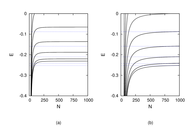
Figure 1: The dependence of the approximate eigenvalues on the number of point potentials for circle with $R=10$ and ${\varepsilon}=0.1$ (a), ${\varepsilon}=0.01$ (b). The dashed lines represent the exact eigenvalues of $-{\Delta}+m$.

Due to the symmetry, the spectrum of $-\Delta+m$ for this specific measure is known; it consists of the essential spectrum $[0,\infty)$ and a finite number of negative eigenvalues, which are all except the lowest one twice degenerate, see [2]. To find the eigenvalues, one has to decompose $L^{2}({\mathbb{R}}^{2})$ into angular momentum subspaces and then to look for solutions of an implicit equation in each of the subspaces. Therefore we can compute and compare both exact and approximate eigenvalues.

Each approximation is characterized by a pair of numbers, ${\varepsilon}>0$ and $N\in{\mathbb{N}}$. In numerical calculations we fix ${\varepsilon}$ and we let $N$ grow. The results for one chosen radius and two different parameters ${\varepsilon}$ are depicted in figure 1, cases (a) and (b) correspond to ${\varepsilon}=0.1$ and ${\varepsilon}=0.01$, respectively. We observe that below some threshold number of points, the approximate discrete spectrum has no resemblance to the exact spectrum. The approximate eigenvalues may be very large negative and their number may be much higher than the number of exact eigenvalues (in figure 1, we even have not plotted all the eigenvalues which exist only for small $N$.)

It appears that for larger ${\varepsilon}$, we get a fast convergence of eigenvalues, however, they are all shifted from the exact ones. The reason is that since we work with fixed ${\varepsilon}$, the limit operator is in fact $-{\Delta}+{\varepsilon}^{2}{\Delta}^{2}+m$ instead of $-{\Delta}+m$. On the contrary, small ${\varepsilon}$ means that one need more points to obtain a qualitatively correct spectrum, but then for a large number of points one gets much closer to the exact spectrum.

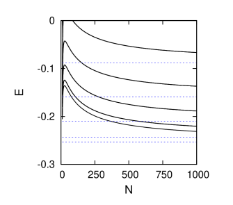
Figure 2: The dependence of the approximate eigenvalues on the number of point potentials for $R=10$, using the standard two-dimensional point potentials. The dashed lines represent the exact eigenvalues of $-{\Delta}+m$.

We can also compare this approximation to [8], where approximating operators were Laplacians with point potentials. Those point potentials are of course different, they are not defined via a quadratic form and cannot be understood as a special case ${\varepsilon}=0$ of section II, instead boundary conditons on wavefunctions are used, see [1]. Figure 2 presents the eigenvalues of Laplacians perturbed by point potentials which converge to $-{\Delta}+m$ with the same measure $m$ as above. We have already mentioned in the introduction that here, we obtain a stronger convergence result than the one in [8]. Moreover, comparing both figures 1 and 2, we see that employing fourth-order differential operators in the approximation may improve significantly the spectral convergence.

Appendix

In section II we have employed Krein’s formula (9). Various forms of this formula can be found in the literature. Let us prove here the one we have used.

Let $f\in L^{2}(dx)$. Since ${\cal E}_{{\varepsilon}}$ and ${\cal E}_{{\varepsilon}}^{\mu}$ are associated to $-{\Delta}+{\varepsilon}^{2}{\Delta}^{2}$ and $-{\Delta}+{\varepsilon}^{2}{\Delta}^{2}+\mu$, respectively, it follows from Kato’s representation theorem that

$${\cal E}_{{\varepsilon},\alpha}(G_{{\varepsilon},\alpha}f,h)=(f,h)={\cal E}_{{\varepsilon},\alpha}^{\mu}((-{\Delta}+{\varepsilon}^{2}{\Delta}^{2}+\mu+\alpha)^{-1}f,h),$$ (38)

for any $h\in H^{2}({\mathbb{R}}^{d})$ and $f\in L^{2}({\mathbb{R}}^{d})$. Moreover we have

$${\cal E}_{{\varepsilon},\alpha}(G_{{\varepsilon},\alpha}^{\mu}\psi,h)=(G_{{\varepsilon},\alpha}^{\mu}\psi,(-{\Delta}+{\varepsilon}^{2}{\Delta}^{2}+\alpha)h)$$

$$= \int\int g_{{\varepsilon},\alpha}(x-y)\bar{\tilde{\psi}}(y)\mu(dy)(-{\Delta}+{\varepsilon}^{2}{\Delta}^{2}+\alpha)h(x)\,dx$$

$$= \int\int g_{{\varepsilon},\alpha}(x-y)(-{\Delta}+{\varepsilon}^{2}{\Delta}^{2}+\alpha)h(x)\,dx\,\bar{\tilde{\psi}}(y)\mu(dy)$$

$$= \int\tilde{h}\bar{\tilde{\psi}}\,\mu(dy),\qquad\psi\in H^{2}({\mathbb{R}}^{d}),\quad h\in D(-{\Delta}+{\varepsilon}^{2}{\Delta}^{2}).$$ (39)

We could change the order of integration in the second step. In fact, as $\mu^{\pm}$ are finite Radon measures and $g_{{\varepsilon},\alpha}$ is square integrable w.r.t. the Lebesgue measure $dx$, the mappings $x\mapsto\int|g_{{\varepsilon},\alpha}(x-y)|\mu^{\pm}(dy)$, ${\mathbb{R}}^{d}\longrightarrow{\mathbb{R}}$, are square integrable w.r.t. $dx$. Since $\tilde{\psi}$ is bounded and $(-{\Delta}+{\varepsilon}^{2}{\Delta}^{2}+\alpha)h\in L^{2}(dx)$ it follows that

$$\int\int|g_{{\varepsilon},\alpha}(x-y)\bar{\tilde{\psi}}(y)|\mu^{\pm}(dy)|(-{\Delta}+{\varepsilon}^{2}{\Delta}^{2}+\alpha)h(x)|dx<\infty$$

and, by Fubini’s theorem, we could change the order of integration in the second step. In the last step we have used (6). Employing Sobolev’s inequality and the fact that $D(-{\Delta}+{\varepsilon}^{2}{\Delta}^{2})$ is dense in $(D({\cal E}_{{\varepsilon}}),{\cal E}_{{\varepsilon},\alpha})$, we can extend (IV) to all functions $\psi,\,h\in D({\cal E}_{{\varepsilon}})$.

Put

$$\phi:=G_{{\varepsilon},\alpha}f-G_{{\varepsilon},\alpha}^{\mu}(I+G_{{\varepsilon},\alpha}^{\mu})^{-1}G_{{\varepsilon},\alpha}f.$$

Then $\phi\in H^{2}({\mathbb{R}}^{d})=D({\cal E}_{{\varepsilon}}^{\mu})$ and (38) and extended (IV) yield

$${\cal E}_{{\varepsilon},\alpha}^{\mu}(\phi,h) = {\cal E}_{{\varepsilon},\alpha}(G_{{\varepsilon},\alpha}f,h)-{\cal E}_{{\varepsilon},\alpha}(G_{{\varepsilon},\alpha}^{\mu}(I+G_{{\varepsilon},\alpha}^{\mu})^{-1}G_{{\varepsilon},\alpha}f,h)$$

$$+\int[G_{{\varepsilon},\alpha}f-G_{{\varepsilon},\alpha}^{\mu}(I+G_{{\varepsilon},\alpha}^{\mu})^{-1}G_{{\varepsilon},\alpha}f\bar{\tilde{]}}\tilde{h}d\mu$$

$$= (f,h)-\int[(I+G_{{\varepsilon},\alpha}^{\mu})^{-1}G_{{\varepsilon},\alpha}f\bar{\tilde{]}}\tilde{h}d\mu$$

$$+\int[(I+G_{{\varepsilon},\alpha}^{\mu})(I+G_{{\varepsilon},\alpha}^{\mu})^{-1}G_{{\varepsilon},\alpha}f-G_{{\varepsilon},\alpha}^{\mu}(I+G_{{\varepsilon},\alpha}^{\mu})^{-1}G_{{\varepsilon},\alpha}f\bar{\tilde{]}}\tilde{h}d\mu$$

$$= (f,h),\qquad h\in H^{2}({\mathbb{R}}^{d}).$$

Due to (10), ${\cal E}_{{\varepsilon},\alpha}^{\mu}$ is a scalar product on $D({\cal E}_{{\varepsilon},\alpha}^{\mu})=H^{2}({\mathbb{R}}^{d})$. Thus (38) and the calculation above imply that $\phi=(-{\Delta}+{\varepsilon}^{2}{\Delta}^{2}+\mu+\alpha)^{-1}f$.

Acknowledgment

This work is partially supported by the Marie Curie fellowship MEIF-CT-2004-009256.

References

[1]
S. Albeverio, F. Gesztesy, R. Høegh–Krohn, H. Holden:
Solvable models in quantum mechanics, second edition.
AMS Chelsea Publ. 2005.
[2]
J.-P. Antoine, F. Gesztesy, J. Shabani: Exactly solvable models of sphere
interactions in quantum mechanics J. Phys. A20 (1987), 3687-3712.
[3]
J. F. Brasche:
On the spectral properties of singular perturbed operators, pp. 65–72
in Z. Ma, M. Röckner, A. Yan (eds.): Stochastic Processes
and Dirichlet forms, de Gruyter 1995.
[4]
J. F. Brasche:
Upper bounds for Neumann – Schatten norms. Potential Analysis14 (2001), 175 – 205.
[5]
J. F. Brasche, P. Exner, Y. Kuperin, P. Šeba:
Schrödinger operators with singular interactions. Journ. Math. Anal. Appl.183 (1994), 112–139.
[6]
J. F. Brasche, R. Figari, A. Teta:
Singular Schrödinger operators
as limits of point interaction Hamiltonians. Potential Analysis8, no.2 (1998),
163 – 178.
[7]
H. L. Cycon, R. G. Froese, W. Kirsch, B. Simon: Schrödinger
Operators. Springer, Berlin–Heidelberg–New York 1987.
[8]
P. Exner, K. Němcová: Leaky quantum graphs: approximations by
point interaction Hamiltonians. J. Phys. A36 (2003), 10173-10193.
[9]
K. S. Murigi: On Eigenvalues of Schrödinger Operators with
-Potentials. Master’s Thesis, Mathematics,
Chalmers University of Technology, Göteborg 2004.
[10]
A. Posilicano: Convergence of distorted Brownian motions and singular
Hamiltonians. Potential Analysis5 (1996), 241-271.
[11]
P. Stollmann, J. Voigt: Perturbation of Dirichlet forms by measures.
Potential Analysis5 (1996), 109-138.