Properties of a fractional derivative Schrödinger type wave equation and a new interpretation of the charmonium spectrum

Abstract

Based on the Caputo fractional derivative the classical, non relativistic Hamiltonian is quantized leading to a fractional Schrödinger type wave equation. The free particle solutions are localized in space. Solutions for the infinite potential well and the radial symmetric ground state solution are presented. It is shown, that the behaviour of these functions may be reproduced by an ordinary Schrödinger equation with an additional potential, which is of the form $V\sim|x|$ for $\alpha<1$, corresponding to the confinement potential, which is introduced phenomenologically to the standard models for a non relativistic interpretation of quarkonium-spectra. The ordinary Schrödinger equation is triple factorized and yields a fractional wave equation with internal $SU(3)$ symmetry. The twofold iterated version of this wave equation shows a direct analogy to the derived fractional Schrödinger equation. The angular momentum eigenvalues are calculated algebraically. The resulting mass formula is applied to the charmonium spectrum and reproduces the experimental masses with an accuracy better than $0.1\%$. Extending the standard charmonium spectrum, three additional particles are predicted and associated with $\Sigma_{c}^{0}(2455)$ and $Y(4260)$ observed recently and one $X(4965)$, not yet observed. The root mean square radius for $\Sigma_{c}^{0}(2455)$ is calculated to be $<\!r\!>\approx 0.3[\text{fm}]$. The derived results indicate, that a fractional wave equation may be an appropriate tool for a description of quark-like particles.

I Introduction

Since NewtonNewton (1669) and LeibnizLeibniz (1675) introduced the concept of infinitesimal calculus, differentiating a function $f(x^{1},...,x^{n})$ with respect to the variable $x^{i}$ is a standard technique applied in all branches of physics. The derivative operator $\partial_{i}$,

$$\partial_{i}=\frac{\partial}{\partial x^{i}}$$ (1)

transforms like a vector, its contraction yields the Laplace-operator, using Einstein’s sum convention

$$\Delta=\partial^{i}\partial_{i}$$ (2)

which is a second order derivative operator, the essential contribution to establish a wave equation, which is the starting point to describe several kinds of wave phenomena.

Until now, in high energy physics the derivative operator has only been used in integer steps. We want to extend the idea of differentation to arbitrary, not necessarily integer steps. A natural generalization is to search for an operator $D_{i}$ by setting

$$D_{i}^{m}=\partial_{i}^{n}$$ (3)

where $m,n$ are integers. Formally, this is solved by extracting the $m$-th root

$$D_{i}=\partial_{i}^{n/m}\qquad\qquad\qquad\qquad m,n\in\mathbb{N}$$ (4)

or, even more general, we will introduce a fractional derivative operator by

$$D_{i}=\partial_{i}^{\alpha}\qquad\qquad\qquad\qquad\quad\alpha\in\mathbb{R}_{+}$$ (5)

with the fractional derivative coefficient $\alpha$ being a positive, real number.

The concept of fractional calculus has stimulated mathematicians since the days of LeibnizLeibniz (1695)-Riemann (1847). In physics, early attempts in the field of applications was studies on non-local dynamics, e.g. anomalous diffusion or fractional Brownian motion Miller (1993),Samko (2003).

During the last decade, remarkable progress has been made in the theory of fractional wave equationsRaspini (2000)-Laskin (2002). RaspiniRaspini (2000),Raspini (2001) has derived a fractional ($\alpha=2/3$) Dirac equation. BaleanuBaleanu (2005) has studied the Euler-Lagrange equations for classical fields and gave the explicit form of a fractional Klein-Gordon-equation and a fractional Dirac-equation, conformal with Raspini’s.

Both studies were based on the use of the Riemann-Liouville (RL) fractional derivative, which is used by many authors working on the field of fractional derivatives.

For practical purposes, the main deficiency of the RL fractional derivative is the fact, that the derivative of a constant function does not vanish. Maybe this is one reason for the fact, that until now, there exists not a single application in the area of high energy physics.

LaskinLaskin (2002) has proposed a hermitean fractional Schrödinger equation, based on Feynman’s path integral approach. His applications are based on the semi classical Bohr-Sommerfeld quantization condition only.

We will use a different approach. We will apply the concept of fractional derivative to derive a fractional Schrödinger type wave equation by a quantization of the classical non relativistic Hamiltonian. We will collect arguments and results which indicate, that this equation is an alternative tool for a appropriate description of the charmonium spectrum, which is normally described by a phenomenological potential.

In the following sections, we will explicitely derive exact solutions for the free particle and for particles in an infinite well potential. We will prove, that these solutions show a behaviour, which may be reproduced by an ordinary Schrödinger equation with an additional linear potential term for $\alpha<1$, indicating that a fractional wave equation and the confinement problem are strongly related.

We will derive a fractional multi-component wave equation via threefold factorization of the ordinary non relativistic Schödinger equation, which contains an internal $SU(3)$ symmetry.

We will then study an analytical mass formula in terms of angular momentum multiplets which will reproduce the experimental masses of the charmonium spectrum within an error of better than $0.1\%$.

We will extend the standard charmonium spectrum and predict new, additional particles.

Finally, we will give a reasonable estimate for the root mean square radius of $\Sigma_{c}^{0}(2455)$.

II Fractional derivative

Let $q=[\alpha]$ be the integer part of $\alpha$ and $f$ a function of n variables $x^{i},\,i=1,...,n$ with $x^{i}>0$. To derive a specific representation of the fractional derivative operator $D_{i}$, defined by (5) we start with the Cauchy integral ${}^{+}I_{i}^{\alpha}$ extended to fractional order

$${}^{+}I_{i}^{\alpha}(x^{i})f(x^{1},...,x^{i},...,x^{n}) =$$ (6)

$$\frac{1}{\Gamma(\alpha)}\int_{0}^{x^{i}}du(x^{i}-u)^{\alpha-1}f(x^{1},...,u, ...,x^{n})$$

a formal split of the partial differential operator into a fractional integral and an integer differential part

$$\partial_{i}^{\alpha} = \partial_{i}^{\alpha-(q+1)}\partial_{i}^{q+1}$$

$$= I_{i}^{(q+1)-\alpha}\partial_{i}^{q+1}$$

leads to the definition of the CaputoCaputo (1967) fractional differential operator ${}^{+}_{c}D$, which is the form we will use.

$${}^{+}_{c}D_{i}(x^{i})f(x^{1},...,x^{i},...,x^{n})=\qquad\qquad$$ (8)

$$\frac{1}{\Gamma(q+1-\alpha)}\int_{0}^{x^{i}}\frac{du}{(x^{i}-u)^{\alpha-q}}\frac{\partial^{q+1}}{\partial u^{q+1}}f(x^{1},...,u, ...,x^{n})$$

For a constant function this fractional derivative vanishes:

$$^{+}_{c}D(x)\,\text{const}=0$$ (9)

For a function of the type

$$f(x)=x^{n\alpha}\qquad\qquad\qquad\qquad\quad n\in\mathbb{N}$$ (10)

the fractional derivative is:

$${}^{+}_{c}D(x)\,x^{n\alpha}=\frac{\Gamma(1+n\alpha)}{\Gamma(1+(n-1)\alpha)}x^{(n-1)\alpha}$$ (11)

For $k>0,x>0$ we are then able to define Caputo-Taylor series of the form

$$f(kx)=\sum_{n=0}^{\infty}a_{n}(kx)^{n\alpha}$$ (12)

The corresponding fractional derivatives are given by:

$${}^{+}_{c}Df(kx)=k^{\alpha}\sum_{n=0}^{\infty}a_{n+1}\frac{\Gamma(1+(n+1)\alpha)}{\Gamma(1+n\alpha)}(kx)^{n\alpha}$$ (13)

Since we intend to use $x$ and the fractional derivative ${}^{+}_{c}D(x)$ on $\mathbb{R}$, the next step is an extension of our definition of $x$ and ${}^{+}_{c}D(x)$ to negative reals $\mathbb{R}_{-}$.

We propose the following mappings for $x\rightarrow\bar{\chi}(x)$ and ${}^{+}_{c}D(x)\rightarrow\bar{D}(x)$:

$$\bar{\chi}(x) = \text{sign}(x)\,|x|^{\alpha}$$ (14)

$$\bar{D}(x) = \text{sign}(x)\,^{+}_{c}D(|x|)$$ (15)

Besides a unique mapping from $\mathbb{R}_{+}$ to $\mathbb{R}_{+}$ and $\mathbb{R}_{-}$ to $\mathbb{R}_{-}$ the behaviour under parity transformations $\Pi$ is well defined:

$$\Pi\bar{\chi}(x) = -\bar{\chi}(x)$$ (16)

$$\Pi\bar{D}(x) = -\bar{D}(x)$$ (17)

With these definitions we are able to define series $f$ on $\mathbb{R}$

$$f(\bar{\chi}(kx))=\sum_{n=0}^{\infty}a_{n}\bar{\chi}^{n}(kx)$$ (18)

with a well defined derivative $\bar{D}$

$$\bar{D}f(\bar{\chi}(kx))=\text{sign}(k)|k|^{\alpha}\sum_{n=0}^{\infty}a_{n+1}\frac{\Gamma(1+(n+1)\alpha)}{\Gamma(1+n\alpha)}\bar{\chi}^{n}(kx)$$ (19)

To construct a Hilbert space on functions $f(\bar{\chi}(kx))$ we first define the integral operator

$$\int_{-x}^{x}du^{\alpha}=\text{sign}(x)^{+}I^{\alpha}(|x|^{\alpha})$$ (20)

with the fractional scalar product

$$<f|g>=\int du^{\alpha}\,f^{*}(\bar{\chi}(ku))\,g(\bar{\chi}(k^{\prime}u))$$ (21)

An expectation value $<\!\hat{O}\!>$ of an operator $\hat{O}$ may consequently be defined with

$$<\!f|\hat{O}|g\!>=\int du^{\alpha}\,f^{*}(\bar{\chi}(ku))\,\hat{O}\,g(\bar{\chi}(k^{\prime}u))$$ (22)

to be

$$<\!\hat{O}\!>=\frac{<\!f|\hat{O}|g\!>}{<\!f|g\!>}$$ (23)

The space coordinates and corresponding derivatives, defined by (14) and (15), are the basic input for our derivation of a fractional non relativistic Schrödinger type wave equation, the corresponding angular momentum operators and caculation of expectation values.

III Quantization of the classical Hamiltonian and free particle solutions

By use of the definitions (14),(15) for the space coordinate and for the fractional derivative, we are able to quantize the Hamiltonian of a classical non relativistic particle and solve the corresponding Schrödinger equation.

We define the following set of conjugated operators on an euclidean space for $N$ particles in space coordinate representation:

$$\hat{P}_{\mu} = \{\hat{P}_{0},\hat{P}_{i}\}=\{i\hbar\partial_{t},-i\left(\frac{\hbar}{mc}\right)^{\alpha}mc\bar{D}_{i}\}$$ (24)

$$= \{i\hbar\partial_{t},-i\left(\frac{\hbar}{mc}\right)^{\alpha}mc\,\,\text{sign}(x^{i})\,^{+}_{c}D(|x^{i}|)\}$$ (25)

$$\hat{X}_{\mu} = \{\hat{X}_{0},\hat{X}_{i}\}=\{t,\left(\frac{\hbar}{mc}\right)^{(1-\alpha)}\frac{\bar{\chi}(x_{i})}{\Gamma(\alpha+1)}\}$$ (26)

$$= \{t,\left(\frac{\hbar}{mc}\right)^{(1-\alpha)}\!\!\!\!\!\!\frac{1}{\Gamma(\alpha+1)}\,\text{sign}(x_{i})|x_{i}|^{\alpha}\}$$

$$\qquad\qquad\qquad\qquad\qquad i=1,...,3N$$

These operators satisfy the following commutator relations on a function set $\{x^{n\alpha}\}$:

$$\left[\hat{X}_{i},\hat{X}_{j}\right] = 0$$ (28)

$$\left[\hat{P}_{i}\,,\hat{P}_{j}\,\right] = 0$$ (29)

$$\left[\hat{X}_{i},\hat{P}_{j}\right] = -i\hbar\delta_{ij}\frac{1}{\Gamma(1+\alpha)}\times$$

$$\left(\frac{\Gamma(1+n\alpha)}{\Gamma(1+(n-1)\alpha)}-\frac{\Gamma(1+(n+1)\alpha))}{\Gamma(1+n\alpha)}\right)$$

$$= -i\hbar\delta_{ij}\,c(n,\alpha)$$ (31)

With these operators, the classical, non relativistic Hamilton function $H_{c}$, which depends on the classical momenta and coordinates $\{p_{i},x^{i}\}$

$$H_{c}=\sum_{i=1}^{3N}\frac{p^{2}_{i}}{2m}+V(x^{1},...,x^{i},...,x^{3N})$$ (32)

is quantized. This yields the Hamiltonian $H^{\alpha}$

$$H^{\alpha}=-\frac{1}{2}mc^{2}\left(\frac{\hbar}{mc}\right)^{2\alpha}\bar{D}^{i}\bar{D}_{i}+V(\hat{X}^{1},...,\hat{X}^{i},...,\hat{X}^{3N})$$ (33)

Thus, a time dependent Schrödinger type equation for fractional derivative operators results

$$H^{\alpha}\Psi = (-\frac{1}{2}mc^{2}\left(\frac{\hbar}{mc}\right)^{2\alpha}\bar{D}^{i}\bar{D}_{i}$$

$$+ V(\hat{X}^{1},...,\hat{X}^{i},...,\hat{X}^{3N}))\Psi=i\hbar\partial_{t}\Psi$$

For $\alpha=1$ this reduces to the classical Schrödinger equation.

III.1 Properties of the momentum operator

We extend the standard series expansion of the exponential function to the fractional case

$$\exp(\alpha,\bar{\chi}(kx)) = \sum_{n=0}^{\infty}\frac{\text{sign}^{n}(kx)|kx|^{\alpha n}}{\Gamma(1+\alpha n)}$$ (35)

$$=\sum_{n=0}^{\infty}\frac{|kx|^{2\alpha n}}{\Gamma(1+2\alpha n)} + \text{sign}(kx)\sum_{n=0}^{\infty}\frac{|kx|^{(2n+1)\alpha}}{\Gamma(1+(2n+1)\alpha)}$$ (36)

$$= \mathfrak{E}_{\alpha}(\bar{\chi}(kx))$$

where $\mathfrak{E_{\alpha}}$ is the Mittag-Leffler functionMittag-Leffler (1903). The functions $\psi=\exp(\alpha,-i\bar{\chi}(kx))$ are eigenfunctions of the momentum operator with the real eigenvalues

$$\hat{P}\psi=\left(\frac{\hbar}{mc}\right)^{\alpha}mc\,\text{sign}(k)\,|k|^{\alpha}\,\psi$$ (37)

The Leibniz product rule, which plays an important role for the standard derivative, is not valid any more for the fractional derivative. Instead, with an arbitrary additional function $R$, we can write:

$$\bar{D}(fg)=(\bar{D}f)g+f(\bar{D}g)+R$$ (38)

For the momentum operator it follows

$$\int du^{\alpha}\,f^{*}(\hat{P}g) = fg-\int du^{\alpha}\,(\hat{P}f^{*})g-\int du^{\alpha}\,R$$ (39)

$$= +\int du^{\alpha}\,(\hat{P}f)^{*}g-\int du^{\alpha}\,R$$

Consequently, neither $\hat{P}$ nor the fractional Schrödinger operator with $H^{\alpha}$ in (III) are hermitean operators.

A direct consequence is the non orthogonality of the calculated eigenfunctions.

In general, hermitean operators are preferred, since their eigenvalues and expectation values are always real. Nevertheless, eigenvalues for momentum, energy and angular momentum as well as expectation values derived with the proposed fractional Schrödinger equation (III) turn out to be real, as will be demonstrated in the following sections.

Anyhow, we doubt, that a fractional operator should always be hermitean. A typical example was the expectation value of the root mean square radius of a free quark. Indeed, any real value would be a contradiction to the experiment.

III.2 Free particle solutions

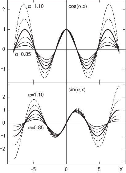
Figure 1: Free particle solutions for the fractional derivative operator Schrödinger type equation, for different values of $\alpha$. Upper part of figure are $\cos(\alpha,x)$, lower part are $\sin(\alpha,x)$ with $\alpha=0.85,0.90,0.95$ (solid thin line), . $\alpha=1$ (solid thick line) and $\alpha=1.05,1.10$ (dashed thin lines) each. For $\alpha=1$ solutions reduce to the standard $\cos(x)$ and $\sin(x)$ functions. For $\alpha<1$ these functions are increasingly located at $x=0$. For $\alpha>1$ the amplitudes increase with increasing $x$.

We will now present the free particle solutions for the fractional Schrödinger type equation (III). We can do this, since for $V(\hat{X}^{i})=0$ the commutator $[\hat{P}_{\mu},H^{\alpha}]$ vanishes and consequently, energy and momentum are conserved.

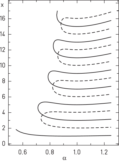
Figure 2: Zeroes of eigenfunctions $\cos(\alpha,\frac{\pi}{2}x)$ (solid lines) and $\sin(\alpha,\frac{\pi}{2}x)$ (dashed lines) of the free particle eigenfunctions. For $\alpha\leq 1/2$ there are no zeroes. For $\alpha=1$ the zeroes are given by $k_{n}=n\in\mathbb{N}$. For $\alpha\geq 1$ an infinite number of zeroes exists.

Let us first consider the one dimensional case. We extend the definition for the standard series expansion for the sine and cosine function

$$\cos(\alpha,x) = \sum_{n=0}^{\infty}\frac{(-1)^{n}\,|x|^{2n\alpha}}{\Gamma(2n\alpha+1)}$$ (40)

$$= \mathfrak{E}_{2\alpha}(-\bar{\chi}^{2}(kx))$$ (41)

$$\sin(\alpha,x) = \text{sign}(x)\sum_{n=0}^{\infty}\frac{(-1)^{n}\,|x|^{(2n+1)\alpha}}{\Gamma((2n+1)\alpha+1)}$$ (42)

$$= \bar{\chi}(kx)\,\mathfrak{E}_{2\alpha,1+\alpha}(-\bar{\chi}^{2}(kx))$$ (43)

where $\mathfrak{E}_{\alpha}$ and $\mathfrak{E}_{\alpha,\beta}$ are Mittag-LefflerMittag-Leffler (1903) and generalized Mittag-Leffler functionsWiman (1905). With these definitions, the following relations are valid:

$$\bar{D}\sin(\alpha,kx) =\text{sign}(k)|k|^{\alpha}\cos(\alpha,kx)$$ (44)

$$\bar{D}\cos(\alpha,kx) =-\text{sign}(k)|k|^{\alpha}\sin(\alpha,kx)$$ (45)

It follows from these relations, that the above functions (40) are the eigenfunctions of the free Schrödinger type equation (III) in one dimension. In the stationary case we get the energy relation

$$E=\frac{1}{2}mc^{2}\left(\frac{\hbar|k|}{mc}\right)^{2\alpha}$$ (46)

This result may easily be extended to the n-dimensional case.

In figure 1 the functions $\sin(\alpha,x)$ and $\cos(\alpha,x)$ are plotted for different values of $\alpha$. While for $\alpha=1$, these functions reduce to the known $\cos(x)$ and $\sin(x)$, which are spread over the whole x-region, for $\alpha<1$ these functions become more and more located at $x=0$ and oscillations are damped, a behaviour, which we know e.g. from the Airy-functions. For $\alpha>1$ the functions amplitude increases for increasing $x$. For $\alpha<1$ these functions are normalizable on $\mathbb{R}$: There exists an upper bound $M$ with

$$\int_{-\infty}^{\infty}dx^{\alpha}\cos(\alpha,kx)\cos(\alpha,k^{\prime}x) < M$$ (47)

$$\int_{-\infty}^{\infty}dx^{\alpha}\sin(\alpha,kx)\sin(\alpha,k^{\prime}x) < M$$ (48)

$$\int_{-\infty}^{\infty}dx^{\alpha}\cos(\alpha,kx)\sin(\alpha,k^{\prime}x) = 0$$ (49)

For $\alpha\geq 1$ this integral is not bound any more, instead a box-normalization with a box size $L$ much larger than the dimensions of the system considered is proposed.

III.3 Particle in an infinite potential well

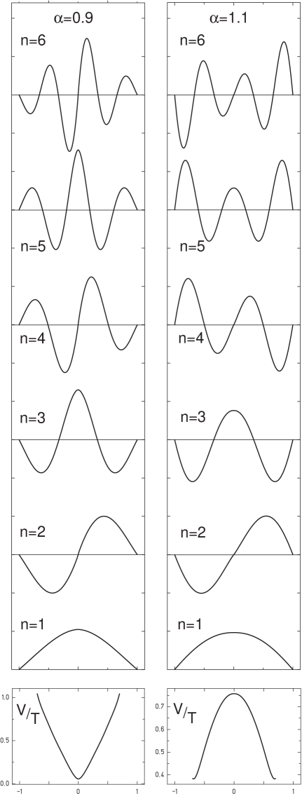
Figure 3: The six lowest eigenfunctions for the one dimensional infinite square well potential, with $\alpha=0.9$ on the left and $\alpha=1.1$ on the right side. Below the corresponding potential for equivalent solutions of the ordinary $(\alpha=1)$ Schrödinger equation, according to (III.5) is plotted. For $\alpha<1$ this potential contains a strong linear admixture, for $\alpha>1$ to potential graph behaves like $\sim 1-x^{2}$

Now we will give the exact eigenfunctions and eigenvalues for a particle confined in an infinite potential well. We first investigate the one dimensional case. Therefore we define the potential $V(x)$

$$V(x)=\begin{cases}0\qquad\,\,\,|x|\leq a\\ \infty\qquad|x|>a\end{cases}$$ (50)

The corresponding boundary condition for the eigenfunctions $\psi(x)$ is:

$$\psi(-a)=\psi(a)=0$$ (51)

In figure 2 the zeroes for the free particle solutions $\cos(\alpha,\frac{\pi}{2}x)$ and $\sin(\alpha,\frac{\pi}{2}x)$ are plotted. For $\alpha\leq 1/2$ there are no zeroes. For the interval $1/2<\alpha<1$ exists only a finite set of zeroes. For $\alpha\geq 1$ an infinite number of zeroes exists.

Let $k^{0}$ be a zero of the free particle solutions. The eigenfunctions of the infinite potential well potential are then given by:

$$\psi_{2n}^{(+)}(x) = \cos(\alpha,\bar{\chi}(k^{0}_{2n}\frac{x}{a}))$$ (52)

$$\psi_{2n+1}^{(-)}(x) = \sin(\alpha,\bar{\chi}(k^{0}_{2n+1}\frac{x}{a}))$$ (53)

where the sign indicates the parity of the states. The normalization condition is

$$\int_{-a}^{a}dx^{\alpha}\psi^{*}_{n}(x)\psi_{n}(x)=1$$ (54)

The energy is then given by

$$e_{n}=\frac{1}{2}\left(\frac{\hbar}{mc}\right)^{2\alpha}mc^{2}|\frac{k^{0}_{n}}{a}|^{2\alpha}$$ (55)

The extension to the N-dimensional case is then

$$\Psi_{n_{1}n_{2}...n_{N}}(x^{1},x^{2},...,x^{N})=\prod_{i=1}^{N}\psi_{n_{i}}(x^{i})$$ (56)

and for the energy

$$E_{n_{1}n_{2}...n_{N}}=\frac{1}{2}\left(\frac{\hbar}{mc}\right)^{2\alpha}mc^{2}\sum_{i=1}^{N}|\frac{k^{0}_{n_{i}}}{a_{i}}|^{2\alpha}$$ (57)

III.4 Radial solutions

In the case of fractional derivative operators there exists no general theory of covariant coordinate transformations until now.

We intend to perform a coordinate transformation from carthesian to hyperspherical coordinates in $\mathbb{R}^{N}$

$$f(x_{1},x_{2},...,x_{N})=f(r,\phi_{1},\phi_{2},...,\phi_{N-1})$$ (58)

The invariant line element in the case $\alpha=1$

$$ds^{2}=g_{ij}dx^{i}dx^{j}\quad i,j=1,...,N$$ (59)

for arbitrary fractional derivative coefficient $\alpha$ may be generalized to

$$ds^{2\alpha}=g_{ij}^{\alpha}dx^{i\alpha}dx^{j\alpha}\quad i,j=1,...,N$$ (60)

Consequently a natural definition of the radial coordinate is given by

$$r^{2\alpha}=\sum_{i=1}^{N}x_{i}^{2\alpha}$$ (61)

We assume the spherical ground state to be independent of the angular variables, square integrable and of positive parity. Therefore an appropriate ansatz is

$$g(N,\alpha,kr)=\sum_{n=0}^{\infty}(-1)^{n}a_{n}(N,\alpha)(|k|r)^{2\alpha n}$$ (62)

or in carthesian coordinates

$$g(N,\alpha,kx_{1},...,kx_{N})=\sum_{n=0}^{\infty}(-1)^{n}a_{n}(N,\alpha)(\sum_{i=1}^{N}|kx|^{2\alpha})^{n}$$ (63)

where the coefficients $a_{n}$ depend on the explicit form of the potential.

For a free particle, a solution on $\mathbb{R}^{N}$ is given with the abbreviation

$$\eta_{j}=\Gamma(1+2\alpha j)/\Gamma(1+2\alpha(j-1))$$ (64)

by the recurrency relation

$$a_{0} = 1$$

$$a_{j} = a_{j-1}/\left((N-1)\,j\,\eta_{1}+\eta_{j}\right)\qquad j=1,2,...$$ (65)

An infinite spherical well is described by the potential

$$V(r)=\begin{cases}0\qquad\,\,\,r\leq r_{0}\\ \infty\qquad r>r_{0}\end{cases}$$ (66)

The corresponding boundary condition for the ground state wave function $g(N,\alpha,r)$ is:

$$g(N,\alpha,r_{0})=0$$ (67)

Let $k^{0}_{\text{sph}}$ be the first zero of the free particle ground state wave function, the ground state wave function for the spherical infinite well potential is given by

$$g(N,\alpha,k^{0}_{\text{sph}}r/r_{0})$$ (68)

and the ground state energy is then given by

$$e_{0}(N,\alpha)=\frac{1}{2}mc^{2}\left(\frac{\hbar}{mc}\frac{k^{0}_{\text{sph}}}{r_{0}}\right)^{2\alpha}$$ (69)

III.5 Remarks on equivalent solutions for the ordinary Schrödinger equation

We have shown, that the free particle solutions and the solutions for the infinite potential square well of the fractional Schrödinger equation for $\alpha<1$ are localized at the origin and for $\alpha>1$ are localized at the boundaries of a given region respectively.

We want to deduce a similar behaviour of these functions in terms of the ordinary $(\alpha=1)$ Schrödinger equation. Let us assume, the eigenfunctions of the fractional Schrödinger equation may be equivalently interpreted as solutions of the ordinary $({\alpha=1})$ Schrödinger equation with an additional potential $V$.

In order to derive the explicit form of this potential, we use the following relation between the eigenfunctions $\Psi_{n}$, temperature $T$ and a given potential $V$, which is derived within the framework of thermodynamics and statistical quantum mechanicsGreiner (2001):

Let $\Psi_{n}$ and $E_{n}$ be the eigenfunctions and energy eigenvalues of the ordinary Schrödinger equation with a given potential $V$:

$$\left(-\frac{\hbar^{2}}{2m}\Delta+V\right)\Psi_{n}=E_{n}\Psi_{n}$$ (70)

As long as the temperature $T$ is large compared to the average level spacing, the relation ($N$ is the normalization constant)

$$\frac{1}{\sqrt{N}}\exp(-V/T) = \frac{\displaystyle\sum_{n=0}^{\infty}\Psi^{*}_{n}\Psi_{n}\exp(-E_{n}/T)}{\displaystyle\sum_{n=0}^{\infty}\exp(-E_{n}/T)}$$

$$T\gg\Delta E_{n}=E_{n+1}-E_{n}$$

is valid.

Since eigenfunctions and eigenvalues for the fractional free particle solutions are known, we therefore are able to deduce the explicit form of such a potential.

In figure 3 the graph of $V/T$ is plotted for $\alpha=0.9$ and $\alpha=1.1$ respectively. For $\alpha=0.9$ the potential contains a dominant linear term $V\sim|x|$ , while for $\alpha=1.1$ a behaviour like $V\sim 1-x^{2}$ may be deduced. Of course, for $\alpha=1$ a potential $V=\text{const}$ results.

The behaviour of the fractional eigenfunctions may alternatively be interpreted, assuming that $\alpha$ is a measure of charge for a particle moving in an homogenously charged background.

For $\alpha>1$, we could assume a charged particle, with charge e.g. $\alpha$ moving in a homogeneous background of charged particles with charge $1-\alpha$. Since for a homogeneously charged sphere and approximately for a charged box too, the potential inside the box is $V\sim-Z(1-r^{2})$ with $Z=1-\alpha$. This obviously would explain a repulsive force. The energetically favoured positions for a particle with charge $\alpha$ indeed were the boundaries of the box.

For $\alpha=1$ the background was neutral and therefore no additional interaction with a particle was present.

For $\alpha<1$ this simple model could explain an attraction, but not the linearity of the potential.

Therefore we obtain the remarkable result, that in the case $\alpha<1$, the free particle solutions of the fractional Schrödinger equation show a behaviour, which is equivalent to the behaviour of solutions of the ordinary Schrödinger equation with an additional linear potential term. In other words, the solutions of a free fractional wave equation with $\alpha<1$ automatically show confinement, a property, which was first observed for quarks.

In order to obtain more properties of the fractional derivative operator Schrödinger equation, we will now calculate the eigenvalues of the angular momentum operator.

IV Classification of angular momentum eigenstates

We define the generators of infinitesimal rotations in the $i,j$-plane ($i,j=1,...,3N$), with $N$ being the number of particles):

$$L_{ij} = \hat{X}_{i}\hat{P}_{j}-\hat{X}_{j}\hat{P}_{i}$$ (72)

$$= -i\hbar\left(\frac{\bar{\chi}(x_{i})}{\Gamma(\alpha+1)}\bar{D}_{j}-\frac{\bar{\chi}(x_{j})}{\Gamma(\alpha+1)}\bar{D}_{i}\right)$$

We will derive the angular momentum eigenvalues algebraically. Thus it is necessary, to apply the commutator relation $[\hat{X}_{i},\hat{P}_{j}]$ (see (III)) repeatedly.

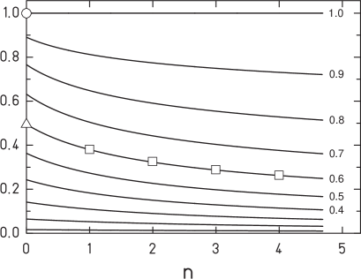
Figure 4: Commutator $[\hat{X}_{i},\hat{P}_{i}]$ from (III) in units of $\hbar$ on the function set $\{x^{n\alpha}\}$ for different values of $\alpha$. The dependence on $n$ is a direct consequence of the fact, that the Leibniz product rule is not valid any more for fractional derivatives. For $\alpha=0.6$ the positions of the successive approximations on $c(n,\alpha)$ according to (73),(74) and (75) are given as circle, triangle and squares.

In figure 4, this commutator $c(n,\alpha)$ is plotted. It shows a smooth dependence on $n$, which we have to eliminate.

Table 1: Eigenvalues in units of $\hbar$ for the angular momentum states of a single particle. $n$ is a counter for the eigenvalues of the Euler operator, eigenvalues for $L_{z}(\alpha)$ and $J^{2}_{c}(\alpha)$ are given for $\alpha=1$, $\alpha=2/3$, $\alpha=0.68$ and $\alpha=0.65$. $J^{2}_{c}(\alpha)$ are listed with c according to (73),(74) and (75).

$n=L_{z}(1)$	$L_{z}(2/3)$	$L_{z}(0.68)$	$J^{2}_{0}(1)$	$J^{2}_{0}(2/3)$	$J^{2}_{0}(0.68)$	$J^{2}_{1}(0.65)$	$J^{2}_{2}(j,0.65)$
0	0	0	0	0	0	0	0
1	1	1	2	2	2	1.604 767	1.478 157
2	1.460 998	1.478 157	6	3.595 515	3.663 108	3.078 892	2.800 590
3	1.860 735	1.894 649	12	5.323 069	5.484 346	4.735 519	4.305 776
4	2.222 222	2.272 597	20	7.160 493	7.437 298	6.539 094	5.961 779
5	2.556 747	2.623 332	30	9.093 704	9.505 205	8.468 379	7.747 796
6	2.870 848	2.953 417	42	11.112 618	11.676 094	10.508 808	9.649 033

Ignoring both, the $n$ and $\alpha$ dependence we set as a lowest order approximation:

$$c_{0}=c(0,1)=1$$ (73)

A more precise statement for $c(n,\alpha)$ can be deduced from the following consideration: Since we will concentrate on the lowest enery levels only , the approximation

$$c_{1}(\alpha)=c(0,\alpha)=1-\frac{1}{\Gamma(1-\alpha)\Gamma(1+\alpha)}$$ (74)

is valid. Of course, this overestimates the commutator for higher values of $n$. Therefore a more sophisticated treatment fixes $c(n,\alpha)$ for a given $j$ to be:

$$c_{2}(j,\alpha)=\frac{\Gamma(1+(j+1)\alpha)}{\Gamma(1+j\alpha)\Gamma(1+\alpha)}-\frac{\Gamma(1+j\alpha)}{\Gamma(1+(j-1)\alpha)\Gamma(1+\alpha)}$$ (75)

We will consider these three cases, which allows an estimate on the validity of the results. Therefore, as long as the commutator does not depend on $n$, $[L_{ij},H^{\alpha}]$ vanishes and angular momentum is conserved. Commutator relations for $L_{ij}$ are isomorph to an extended fractional $SO^{\alpha}(3N)$ algebra:

$$[L_{ij},L_{mn}]=i\hbar\,c(\alpha)\,(\delta_{im}L_{jn}+\delta_{jn}L_{im}-\delta_{in}L_{jm}-\delta_{jm}L_{in})$$ (76)

Consequently, we can proceed in a standard way Louck (1972), by defining the Casimir operators

$$\Lambda_{k}^{2}=\frac{1}{2}\sum_{i,j}^{k}(L_{ij})^{2}\qquad,\qquad k=2,...,3N$$ (77)

which indeed fulfill the relations $[\Lambda_{3N}^{2},L_{ij}]=0$ and successively $[\Lambda_{k}^{2},\Lambda_{k^{\prime}}^{2}]=0$. Consequently the successive group chain

$$SO^{\alpha}(3N)\supset SO^{\alpha}(3N-1)\supset\ldots\supset SO^{\alpha}(3)\supset SO^{\alpha}(2)$$ (78)

is established. The explicit form of the Casimir operators is given by

$$\Lambda_{k}^{2}=+\hat{X}^{i}\hat{X}_{i}\hat{P}^{j}\hat{P}_{j}-i\hbar c(\alpha)\,(\delta_{i}^{i}-1)\hat{X}^{j}\hat{P}_{j}-\hat{X}^{i}\hat{X}^{j}\hat{P}_{i}\hat{P}_{j}$$ (79)

We introduce a generalization of the homogeneous Euler operator for fractional derivative operators

$$J_{e}^{k}(\alpha)=\bar{\chi}(x^{i})/\Gamma(1+\alpha)\,\bar{D}_{i}$$ (80)

With the generalized Euler operator the Casimir-operators are:

$$\Lambda_{k}^{2}=+\hat{X}^{i}\hat{X}_{i}\hat{P}^{j}\hat{P}_{j}+\hbar^{2}\left(c(\alpha)\,(k-2)J_{e}^{k}+J_{e}^{k}J_{e}^{k}\right)$$ (81)

Now we define a Hilbert space $\mathfrak{H}_{\alpha}$ of all homogeneous functions $f$, which satisfy the Laplace equation $\bar{D}^{i}\bar{D}_{i}f=0$ and are normalized in the interval $[-1,1]$:

$$\mathfrak{H}_{\alpha}=\{f:f(\lambda\vec{x})=\lambda^{n\alpha}f(x);\;\bar{D}^{i}\bar{D}_{i}f=0\}\qquad n\in\mathbb{N}$$ (82)

This is the quantization condition. It guarantees, that solutions are regular at the origin.

On this Hilbert space, the generalized Euler operator $J_{e}^{k}(\alpha)$ is diagonal and has the eigenvalues

$$l_{k}(\alpha,n)=\begin{cases}0&\text{for}\,\,n=0\\ \frac{\displaystyle 1}{\displaystyle\Gamma(\alpha+1)}\frac{\displaystyle\Gamma(n\alpha+1)}{\displaystyle\Gamma((n-1)\alpha+1)}&\text{for}\,\,n=1,2,3,...\\ \end{cases}$$ (83)

This is the main result of our derivation.

We want to emphasize, that these eigenvalues are different from the degree of homogenity in the general case $\alpha\neq 1$, or, in other words: only in the case of $\alpha=1$ the homogenity degree $n$ of the polynoms considered coincides with the eigenvalues of $J_{e}^{k}(\alpha=1,n)$.

Once the eigenvalues of the generalized Euler operator are known, the eigenvalues of the Casimir-operators $\Lambda_{2},\Lambda_{k}^{2}$ are known, too:

$$\Lambda_{2}f = \hbar l_{2}(\alpha,n)f$$ (84)

$$\Lambda_{k}^{2}f = \hbar^{2}l_{k}(\alpha,n)(l_{k}(\alpha,n)+c(\alpha)\,(k-2))f$$ (85)

with

$$l_{k}\geq l_{k-1}\geq...\geq\mid\pm l_{2}\mid\geq 0$$ (86)

For the case of only one particle ($N=1$), we can introduce the quantum numbers j and m, which now denote the j-th or m-th eigenvalue of the Euler operator. The eigenfunctions are fully determined by these two quantum numbers $f=\mid\!jm\!>$

With the definitions $L_{z}=L_{12}$ and $J^{2}=L_{12}^{2}+L_{13}^{2}+L_{23}^{2}$ it follows

$$L_{z}\mid\!jm\!> = \hbar l_{2}(\alpha,m)\mid\!jm\!>$$

$$\qquad\qquad m=0,\pm 1,\pm 2,...,\pm j$$

$$J^{2}\mid\!jm\!> = \hbar^{2}l_{3}(\alpha,j)\left(l_{3}(\alpha,j)+c(\alpha)\right)\mid\!jm\!>$$

$$\qquad\qquad j=0,+1,+2,...$$

Please note the fact that $L_{z}$ remains unchanged for any choice of constant $c(\alpha)$, only $J^{2}$ changes.

In table 1 the first seven eigenvalues of $L_{z}$ and $J^{2}$ for a single particle are listed for $\alpha=1$, $\alpha=2/3,0.68$ and $\alpha=0.65$ and different approximations for $c(\alpha)$. For $\alpha\neq 1$ the eigenvalues of the generalized Euler operator are not equally spaced any more. For $\alpha<1$ the stepsize is strongly reduced. Since the generalized Euler operator eigenvalues contribute quadratically into the definition $J^{2}$, the energy of higher total angular momenta is reduced increasingly.

We have derived the full spectrum of the angular momentum operator for the fractional derivative operator Schrödinger type wave equation by use of standard algebraic methods.

We will get additional information about the properties of this wave equation, if we consider its factorized pendant. We present some results in the next section.

V Results for the factorization of a non relativistic second order differential equation

Linearization of a relativistic second order wave equation was first considered by DiracDirac (1928). Starting with the relativistic Klein-Gordon equation his derived Dirac equation gave a correct description of the spin and the magnetic moment of the electron.

The concept of linearization is important, since it provides a well defined mechanism to add an additional SU(2) symmetry to a given set of symmetry properties of a second order wave equation.

Since linearization may be interpreted as a special case of factorization, namely to 2 factors, a natural generalization is a factorization to n factors.

In 2000, RaspiniRaspini (2000) proposed a Dirac-like equation with fractional derivatives of order 2/3 and found the corresponding matrix algebra to be related to generalized Clifford algebras; in 2002 Z$\acute{\text{a}}$vada Zavada (2002) generalized Dirac’s approach, and found, that relativistic covariant equations generated by taking the n-th root of the Klein-Gordon or d’Alembert operator ( $\square^{1/n}$) are fractional wave equations with an additional SU(n) symmetry.

These results indicate, that fractional order wave equations may be appropriate candidates for a description of particles, which own a SU(n) symmetry. The case $n=3$, which corresponds to a triple factorization is therefore important for a description of particles with a SU(3) symmetry.

Whether or not a factorization of non relativistic wave equations leads to similar results, has not been examined yet.

In 1967, Levy-LeblondLevy-Leblond (1967) has linearized the non relativistic Schrödinger equation and obtained a linear wave equation with an additional SU(2) symmetry, but until now his approach has not been extended to higher fractional order.

In order to obtain additional information on the inherent symmetries of the fractional Schrödinger equation, which we proposed in (III), we therefore derive in the following section the explicit form of a fractional operator, which evolves from a triple factorization of the ordinary Schrödinger equation:

V.1 Triple factorization of the non relativistic Schrödinger equation

We intend to derive a fractional operator $R$, which, iterated 3 times, conforms with the ordinary, non relativistic Schrödinger operator:

$$RR^{\prime}R^{\prime\prime}=\left(-\frac{\hbar^{2}}{2m}\Delta-i\hbar\partial_{t}\right)\bm{1}_{n}$$ (89)

where $\bm{1}_{n}$ is the $n\times n$ unit matrix.

We use the following ansatz:

$$R = aA\partial^{\alpha_{t}}_{t}+bB^{i}\partial^{\alpha_{i}}_{i}+cC$$ (90)

$$R^{\prime} = aA^{\prime}\partial^{\alpha_{t}}_{t}+bB^{\prime i}\partial^{\alpha_{i}}_{i}+cC^{\prime}$$ (91)

$$R^{\prime\prime} = aA^{\prime\prime}\partial^{\alpha_{t}}_{t}+bB^{\prime\prime i}\partial^{\alpha_{i}}_{i}+cC^{\prime\prime}$$ (92)

with matrices $A,A^{\prime},A^{\prime\prime},B,B^{\prime},B^{\prime\prime},C,C^{\prime},C^{\prime\prime}$, fractional derivative coefficients for time and space derivative $\alpha_{t},\alpha_{i}$ and scalar factors $a,b,c$, which will be determined in the following. According to Z$\acute{\text{a}}$vada Zavada (2002), we define a triad of unitary, traceless $3\times 3$ Pauli type matrices, which span a subspace of $SU(3)$ with

$$x_{k}=\exp({\frac{2\pi i}{3}\,k})\qquad k=1,2,3$$ (93)

an explicit representation is

$$\sigma^{1} = \begin{pmatrix}0&x_{1}&0\\ 0&0&x_{2}\\ x_{3}&0&0\\ \end{pmatrix}$$ (94)

$$\sigma^{2} = \begin{pmatrix}0&x_{2}&0\\ 0&0&x_{1}\\ x_{3}&0&0\\ \end{pmatrix}$$ (95)

$$\sigma^{3} = \begin{pmatrix}x_{1}&0&0\\ 0&x_{2}&0\\ 0&0&x_{3}\\ \end{pmatrix}$$ (96)

These matrices obey an extended Clifford algebra

$$\sum_{\text{all Permutations}}\sigma^{i}\sigma^{j}\sigma^{k}=6\,\delta^{ijk}\quad i,j,k=1,2,3$$ (97)

Let $\otimes$ denote the outer product of any two matrices. In order to describe a single particle with the coordinates $\{t,x,y,z\}$, we define the following 4 $\gamma$ matrices, with dimension $9\times 9$:

$$\gamma^{0} = \bm{1}_{3}\otimes\sigma^{3}$$ (98)

$$\gamma^{i} = \sigma^{i}\otimes\sigma^{1}\qquad i=1,2,3$$ (99)

Now we are able to specify the above introduced matrices:

$$A = \frac{1}{\sqrt{3}}(\gamma^{0}-x_{1}\,\bm{1}_{9})$$ (100)

$$A^{\prime} = \frac{1}{\sqrt{3}}(\gamma^{0}-x_{2}\,\bm{1}_{9})$$ (101)

$$A^{\prime\prime} = \frac{1}{\sqrt{3}}(\gamma^{0}-x_{3}\,\bm{1}_{9})$$ (102)

$$B^{i} = \gamma^{i}$$ (103)

$$B^{\prime i} = \gamma^{i}$$ (104)

$$B^{\prime\prime i} = \gamma^{i}$$ (105)

$$C = x_{1}\,\bm{1}_{3}\otimes\begin{pmatrix}1&0&0\\ 0&0&0\\ 0&0&0\\ \end{pmatrix}$$ (106)

$$C^{\prime} = x_{2}\,\bm{1}_{3}\otimes\begin{pmatrix}0&0&0\\ 0&1&0\\ 0&0&0\\ \end{pmatrix}$$ (107)

$$C^{\prime\prime} = x_{3}\,\bm{1}_{3}\otimes\begin{pmatrix}0&0&0\\ 0&0&0\\ 0&0&1\\ \end{pmatrix}$$ (108)

with these specifications $R\,R^{\prime}R^{\prime\prime}$ yields

$$R\,R^{\prime}R^{\prime\prime}=\left(a^{2}c\,\partial^{2\alpha_{t}}_{t}+b^{3}\sum_{i=1}^{3}\partial^{3\alpha_{i}}_{i}\right)\bm{1}_{9}$$ (109)

A term by term comparison with the nonrelativistic Schrödinger operator determines the fractional derivative coefficients:

$$\alpha_{t} = 1/2$$ (110)

$$\alpha_{i} = 2/3$$ (111)

and the scalar factors:

$$a = (-i\hbar)^{1/2}\left(\frac{1}{mc^{2}}\right)^{1/6}$$ (112)

$$b = -\left(\frac{\hbar^{2}}{2m}\right)^{1/3}$$ (113)

$$c = (mc^{2})^{1/3}$$ (114)

Finally, according to (14) and (8), we extend the derivative operator on $\mathbb{R}$ via:

$$\partial_{\mu}\rightarrow\text{sign}(x^{\mu})\,^{+}_{c}D(|x^{\mu}|)$$ (115)

Thus the fractional operators $R,\,R^{\prime},R^{\prime\prime}$ are completely determined. As a remarkable fact we note the different fractional derivative coefficients for the fractional time and space derivative.

We therefore have proven, that the resulting SU(3) symmetry is neither a consequence of a relativistic treatment nor is it a specific property of linearization (which means, specific to first order derivatives of time and space respectively).

It is a consequence of the triple factorization solely.

We want to emphasize, that the factorization not only determines the symmetry group of the $\gamma$-matrices used, but also determines the dynamics of the system, forcing e.g. for a SU(3) symmetry fractional time ($\alpha_{t}=1/2$) and space derivatives($\alpha_{i}=2/3$).

Thus, the result of factorization shows two important properties: It yields an additional SU(n) symmetry and simultaneously the corresponding dynamics. Applied to QCD, this seems more consistent than the standard concept based on Yang-Mills field theories, where an arbitrary non abelian symmetry group gauge field, which first has to be deduced from experimental data to be a SU(3) symmetry is coupled to a symmetry independent dynamical (e. g. Dirac) field, neglecting a possible influence of the symmetry onto the dynamics.

In that sense, the fractional operator $R$, defined in (90), would be an alternative starting point for a pure, non relativistic QCD, since it contains a consistent description of both, symmetry and dynamics of a pure SU(3) symmetry, without any additional SU(2) admixture.

Finally, besides the fractional wave equation operator $R$ and the triple iterated $R\,R^{\prime}R^{\prime\prime}$, which corresponds to the ordinary Schrödinger operator, an additional type of wave equation, the twofold iterated $R\,R^{\prime}$ emerges, which reads:

$$cR\,R^{\prime}=a^{2}cAA^{\prime}\partial_{t}+b^{2}cB^{i}B^{j}\partial^{2/3}_{i}\partial^{2/3}_{j}+\text{additional terms}$$ (116)

or, inserting the factors:

$$S^{(2)} = -i\hbar AA^{\prime}\partial_{t}-\frac{1}{2}(\frac{\hbar}{mc})^{4/3}mc^{2}\,(\frac{1}{2})^{1/3}\,B^{i}B^{j}\partial^{2/3}_{i}\partial^{2/3}_{j}$$ (117)

$$+\text{additional terms}$$

Obviously $S^{(2)}$ and the fractional Schrödinger equation (III), we derived in section III, are closely related.

$H^{\alpha}$ seems nothing else but a scalar version of $S^{(2)}$ for the special case $\alpha=2/3$. Therefore, examination of the properties of the scalar fractional Schrödinger equation (III) with $\alpha=2/3$ should reveal some properties of an inherent $SU(3)$ symmetry.

Summarizing all facts collected, we assume, that the fractional derivative operator Schrödinger type wave equation with $\alpha=2/3$ is an appropriate candidate for a non relativistic description of particles with quark-like properties.

VI Interpretation of the Charmonium spectrum

In the previous sections we have introduced the concept of fractional derivative operators and discussed some properties of the resulting non relativistic fractional Schrödinger type equation and its factorized pendant.

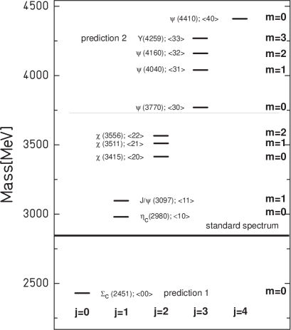
Figure 5: Charmonium spectrum. All observed particles are given with their name, experimental mass fromEidelman (2004) and the proposed $SO^{\alpha}(3)$ conforming quantum numbers j and m, which are the j-th and m-th eigenvalue of the generalized Euler operator. Predicted particles are: in the lower part of the spectrum denoted as prediction 1 $<\!00\!>$ associated with $\Sigma_{c}^{0}(2455)$ and in the upper part prediction 2 $<\!33\!>$ associated with Y(4260).

We have developed a new theoretical concept, which fulfills at least the following three demands: First, available experimental data will be reproduced with a reasonable accuracy. Second, it will give new insights on underlying symmetries and properties of the objects under consideration. Third, we will make predictions, which can be proven by experiment.

None of our results, presented so far, does require any information from QCD or a similar theory. All our statements could have been made in the 1930s already, even though they would have been highly speculative. Today, we are in the comfortable position, that there are enough experimental data, our predictions can be compared with.

A promising candidate is the charmonium spectrumEichten (1976).

In the upper part of figure 5 we have displayed all experimentally observed charmonium-states with experimental masses, which are normally compared with results from a potential model, which tries to simulate confinement and attraction by fitting a model potentialEichten (1976),Krammer (1979).

We will assume, that this spectrum is a single particle spectrum for a particle, whose properties are described by the free fractional Schrödinger type equation(III). We suppose, the system is rotating in a minimally coupled field, which causes a magnetic field $B_{j}$. This leads to the following Hamiltonian H or mass formula

$$H(j,m)\mid\!jm\!>=\left(\kappa J^{2}/\hbar^{2}+B_{j}L_{z}/\hbar+m_{0}c^{2}\right)\mid\!jm\!>$$ (118)

where $\kappa$, $B_{j}$ and $m_{0}c^{2}$ will be adjusted to the experimental data.

The eigenfunctions $\mid\!jm\!>$ are modified spherical harmonics with $D^{i}D_{i}\mid\!jm\!>=0$, the eigenvalues for $J^{2}$ and $L_{z}$ are given by (IV),(IV) and are listed in table 1.

A first remarkable observation is the fact, that states with $L_{z}<0$ are missing in the experimental spectrum. Only right-handed particles are realized.

This may be due to the fact, that actually $L_{z}^{2}$ is a Casimir-Operator of $SO^{\alpha}(2)$, while $L_{z}$ is not and therefore the multipletts should more precisely be classified according to the $m^{2}$ quantum number in the general case $\alpha\neq 1$. Consequently in the following we will work with $L_{z}\geq 0$.

To check the influence of our approximations (73),(74) and (75) of $c(\alpha)$ given in (III) we will proceed in two steps: First, we will consider the case $c_{0}=1$. In a second step, we will test the influence of the successive approximations for $c(\alpha)$ on the accuracy of the proposed mass formula with least square fits on the charmonium spectrum.

VI.1 Interpretation of the charmonium spectrum in the case $c_{0}=1$

We first consider the case $c(\alpha)=1$. The corresponding $J^{2}$ and $L_{z}$ values used are listed in table 1 as $L_{z}(\alpha)$ and $J^{2}_{0}(\alpha)$.

The first crucial test is the verification of the correct value of the non trivial $m=2$ quantum number which corresponds to the $n=2$ eigenvalue of the generalized Euler operator.

For the set of $\chi$-particles ($j=2$) (experimental masses and errors are taken from Eidelman (2004)), we obtain:

$$L_{z}(j=2,m=2)_{\text{exp}} = \frac{\chi(3556)\!<\!22\!>-\chi(3415)\!<\!20\!>}{\chi(3511)\!<\!21\!>-\chi(3415)\!<\!20\!>}$$ (119)

$$= 1.478\pm 0.007$$

Thus, an $\alpha$ from the experimental spectrum is deduced:

$$\alpha_{\text{exp}}^{j=2}=0.680\pm 0.006$$ (120)

Which is remarkably close to the theoretically expected $\alpha_{\text{th}}=2/3$.

An alternative approach to determine the experimental value for $\alpha$ or the $m=2$ quantum number repectively, follows from the set of $\Psi$-particles ($j=3$):

$$L_{z}(j=3,m=2)_{\text{exp}} = \frac{\Psi(4160)\!<\!32\!>-\Psi(3770)\!<\!30\!>}{\Psi(4040)\!<\!31\!>-\Psi(3770)\!<\!30\!>}$$ (121)

$$= 1.44\pm 0.09$$

A second experimental $\alpha$ is obtained:

$$\alpha_{\text{exp}}^{j=3}=0.65\pm 0.08$$ (122)

Within experimental errors, both values are identical. This observation supports the assumption, that the spectrum may be interpreted using one unique $\alpha$.

According to our level scheme, the $\Psi\!<\!33\!>\!$ state is missing in the standard charmonium spectrum. Using $\alpha_{\text{exp}}^{j=2}=0.680$ and $L_{z}(\alpha,m)$ from table 1 the predicted mass is:

$$\Psi\!\!<\!\!33\!\!>\! = \frac{L_{z}(\alpha,m=3)}{L_{z}(\alpha,m=2)}(\Psi(4160)\!\!<\!\!32\!\!>-\Psi(3770)\!\!<\!30\!\!>)$$ (123)

$$= 4268\pm 22[\text{MeV}]$$

In june 2005, the Babar collaboration announced the discovery of a new charmonium state named Y(4260) Aubert (2005). The reported mass of 4259$[\text{MeV}]$ is in excellent agreement with our mass prediction for $\Psi\!<\!33\!>$. Therefore, we associate the predicted particle with $Y(4260)$.

Next we will determine the constants $m_{0}c^{2}$ and $\kappa$ in (118).

We choose the two lowest experimental states of the standard charmonium spectrum, $\eta_{c}(2980)\!<\!10\!>$ and $\chi(3415)\!<\!20\!>$. With $\alpha_{\text{exp}}^{j=2}=0.680$ and $J^{2}_{0}(\alpha,j)$ from table 1 we obtain a set of equations

$$m_{0}c^{2}+2\kappa = \eta_{c}(2980)\!<\!10\!>$$ (124)

$$m_{0}c^{2}+3.663108\kappa = \chi(3415)\!<\!20\!>$$ (125)

which determine

$$m_{0}c^{2} = 2455\pm 3[\text{MeV}]$$

$$\kappa = 262.4\pm 0.9[\text{MeV}]$$ (126)

Our level scheme predicts a particle with quantum numbers $<\!00\!>$, which is beyond the scope of charmonium potential models. According to our mass formula, it has a predicted mass of $<\!00\!>=2455\pm 3[\text{MeV}]$.

Since this is a low lying state, it should already have been observed. Indeed, there exists an appropriate candidate, the $\Sigma_{c}^{0}(2455)\!<\!00\!>$ baryon, with an experimental mass of $2452.2[\text{MeV}]$. This is a charmed baryon with quark content (ddc).

The minimal difference of only $2.8[\text{MeV}]$ between predicted and experimental mass of the $\Sigma_{c}^{0}(2455)\!<\!00\!>$ particle indicates, that the assumed fractional $SO^{\alpha}(3)$ symmetry is fulfilled exactly.

Obviously, the fractional $SO^{\alpha}(3)$ multipletts describe mesonic and baryonic states of the charm-quark simultaneously.

Due to its experimentally observed properties, the internal structure of the $Y(4260)\!\!<\!\!33\!\!>$ particle is subject of actual discussionZhu (2005). Besides being a conventional $c\bar{c}$ state, it could alternatively be a tetraquark with constituents $(u\bar{u}c\bar{c})$ or a hybrid charmonium.

Finally we have only one experimental candidate for $j=3$ and $j=4$ respectively. With parameters (VI.1) using the mass formula (118) we obtain the theoretical values

$$\Psi(3770)\!<\!30\!>_{th} = 3894\pm 8[\text{MeV}]$$ (127)

$$\Psi(4410)\!<\!40\!>_{th} = 4406\pm 10[\text{MeV}]$$ (128)

For $j=3$ the calculated mass (127) differs by $124[MeV]$ from the experimental value.

On the other hand, the theoretical $\Psi(4410)\!<\!40\!>$ mass (128) matches exactly with the experimental value within the experimental errors.

This indicates, that the particles for $j=3$, observed in experiment, carry an additional property, which reduces the mass by the amount of e.g. a pion. Of course, if we add an additional $(\Delta\tau)\delta_{j3}$ term to the proposed mass formula, we can shift these levels by the necessary amount.

Summarizing these results, the charmonium spectrum reveals an underlying $SO^{\alpha}(3)$ symmetry, which agrees with the predictions of our theory in the case of $\alpha\approx 2/3$. The eigenvalues of the generalized Euler operator conform within experimental errors with experimental data. Extending the standard charmonium spectrum, two additional particles have been predicted and associated with $\Sigma_{c}^{0}(2455)$ and $Y(4260)$ observed recently.

VI.2 Least square fits of the charmonium spectrum

Table 2: Optimum parameter sets for a fit of the experimental charmonium spectrum with mass formula (129) in units $[$MeV$]$. Errors $\Delta m$ are given for the subset $m=0$ and the full spectrum $\Delta m_{all}$. The first row corresponds to $\alpha=2/3$ fixed, the following three rows correspond to the three approximations for $c_{0}$,$c_{1}$ and $c_{2}$ according to (73),(74) and (75) with $\alpha$ optimized. In table 3 resulting theoretical masses and errors are listed.

$\alpha$	$c(\alpha)$	$m_{0}c^{2}$	$\kappa$	$B_{1}$	$B_{2}$	$B_{3}$	$\Delta\tau$	$\Delta m_{m=0}$	$\Delta m_{all}$	comment
2/3	1.00	2439.33	274.66	108.25	87.00	263.69	-129.04	5.68	8.98	$\alpha$ fixed
0.681	1.00	2451.26	263.83	117.98	93.39	259.16	-124.48	1.86	2.02	$\alpha$ variation
0.647	0.545	2452.67	336.16	119.79	95.72	270.19	-129.00	1.14	1.15	$\alpha$ variation
0.649	c(j,$\alpha$)	2451.90	367.41	116.13	98.37	269.46	-124.39	0.73	0.79	$\alpha$ variation

In the previous section we gave an interpretation of the charmonium spectrum for the case $c(\alpha)=1$. We found, that the spectrum may be described quantitatively, using the proposed mass formula for $\alpha=0.680$.

Extending the mass formula (118) including a correction term for the $j=3$ multiplett, we use

$$H(j,m)\!\mid\!jm\!>=\kappa J^{2}/\hbar^{2}+B_{j}L_{z}/\hbar+m_{0}c^{2}+\delta_{3\,j}\Delta\tau\!\mid\!jm\!>$$ (129)

to find a fit on the experimental charmonium spectrum.

To prove, that for $c_{0}=1$, $\alpha=0.68$ indeed is the appropriate choice for an interpretation of the charmonium spectrum, we minimized errors with respect to $\alpha$ and obtained $\alpha=0.681$. In table 2 the optimum parameter sets for $\alpha=2/3$ and $c_{0},c_{1},c_{2}$ and resulting errors are tabulated.

For $c_{1}(\alpha)$ from (74), $\alpha=0.68$ is not the optimum choice any more. We therefore minimized errors with respect to $\alpha$, finding $\alpha=0.647$ for this case.

For $c_{2}(j,\alpha)$ from (75), we observe a minimal shift in $\alpha$, finding $\alpha=0.649$ for this case. This indicates, that a more sophisticated treatment of $c(\alpha)$ will only cause neglible changes for $\alpha$ and corresponding parameter sets.

Comparing the optimum parameter sets, the changes in the treatment of $c(\alpha)$ are mainly absorbed by the parameter $\kappa$. Parameter $\Delta\tau$ remains remarkably constant. This supports interpretation for this parameter to be a $j=3$ specific quantum number.

A comparison of experimental with calculated masses, based on the optimum parameter sets, is given in table 3. Mass differences are less than $0.1\%$ and decreasing for $c_{0},c_{1},c_{2}$.

With the optimum parameter sets we can predict the mass of the $<50>$ state to be

$$X\!<\!50\!>_{\text{th}}=4965\pm 10[\text{MeV}]$$ (130)

This state has not been observed in experiments yet.

We conclude, that the proposed $SO^{\alpha}(3)$ symmetry is fulfilled exactly. The values of $\alpha=0.68$ and $\alpha=0.65$ resulting from the least square fits are close to , but differ significantly from the theoretically expected $\alpha=2/3$. This indicates, that the inherent $SU(3)$ symmetry is almost fulfilled exactly, with a difference of only $2\%$.

Table 3: Comparison of experimental and calculated masses according to mass formula (129) with optimized parameter sets listed in table 2 in units $[\text{MeV}]$. The last row lists predicted theoretical masses for $X\!<\!\!50\!\!>$.

			$\alpha=2/3,\,c_{0}=1$		$\alpha=0.68,\,c_{0}=1$		$\alpha=0.647,\,c_{1}(\alpha)$		$\alpha=0.649,\,c_{2}(j,\alpha)$
$<\!jm\!>$	symbol	$m_{exp}$	$m_{th}$	$\Delta m_{th}$	$m_{th}$	$\Delta m_{th}$	$m_{th}$	$\Delta m_{th}$	$m_{th}$	$\Delta m_{th}$
$<\!00\!>$	$\Sigma_{c}^{0}$	2452.2	2439.33	-12.87	2451.26	-0.93	2452.67	0.47	2451.90	-0.30
$<\!10\!>$	$\eta_{c}$	2979.6	2988.66	9.05	2978.94	-0.66	2977.12	-2.47	2980.78	1.18
$<\!11\!>$	$J/\Psi$	3096.9	3096.92	0	3096.92	0	3096.92	0	3096.92	0
$<\!20\!>$	$\chi_{0}$	3415.2	3426.89	11.70	3417.80	2.60	3417.15	1.95	3413.65	-1.54
$<\!21\!>$	$\chi_{1}$	3510.6	3513.89	3.30	3511.19	0.60	3512.87	2.27	3512.03	1.43
$<\!22\!>$	$\chi_{2}$	3556.3	3554.00	-2.26	3555.85	-0.40	3554.68	-1.58	3555.26	1.00
$<\!30\!>$	$\Psi$	3770	3772.35	2.34	3773.92	3.92	3770.17	0.17	3770.41	0.41
$<\!31\!>$	$\Psi$	4040	4036.04	-3.95	4033.08	-6.91	4040.37	0.37	4039.87	-0.13
$<\!32\!>$	$\Psi$	4160	4157.60	-2.39	4157.02	-2.98	4158.39	-1.61	4158.30	-1.70
$<\!33\!>$	$Y(4260)$	4259	4263.01	4.01	4264.98	5.97	4260.08	1.07	4260.42	1.42
$<\!40\!>$	$\Psi$	4415	4406.07	-8.92	4413.80	-1.20	4414.36	-0.64	4415.22	0.22
$<\!50\!>$	$X$		4937.06		4959.54		4957.54		4969.07

VI.3 Size estimate for $\Sigma_{c}^{0}$

Up to now we have treated $m_{0}c^{2}$ as a simple parameter of the proposed mass formula. As a result of our discussion above, we associate $H(0,0)=m_{0}c^{2}$ with the mass of $\Sigma_{c}^{0}$. If $H(j,m)$ was the solution of the Schrödinger equation with a given potential V, then $H(0,0)$ would be interpreted as the zero point energy in this potential plus the rest mass of its constituents.

We intend to estimate the size of $\Sigma_{c}^{0}$. Therefore we will calculate the expectation value $<\!\hat{r}\!>$ of the radius operator $\hat{r}$, which is given by

$$\hat{r} = \sqrt{\hat{X}_{1}^{2}+\hat{X}_{2}^{2}+\hat{X}_{3}^{2}}$$ (131)

$$= \left(\frac{\hbar}{mc}\right)^{1-\alpha}\!\!\frac{1}{\Gamma(1+\alpha)}\sqrt{x_{1}^{2\alpha}+x_{2}^{2\alpha}+x_{3}^{2\alpha}}$$ (132)

For a first estimate, we choose the infinite square well potential(50). The energy eigenvalues are given by (57). Therefore

$$\Sigma_{c}^{0} = (2m_{d}+m_{c})c^{2}+E_{0}(N=3,\alpha)$$

$$= (2m_{d}+m_{c})c^{2}+\frac{3}{2}\left(\frac{\hbar}{m_{c}c}\right)^{2\alpha}m_{c}c^{2}|\frac{k^{0}_{0}}{a}|^{2\alpha}$$

determines the half boxsize $a$. The wave function was defined in (40). Therefore with the abbreviations

$$dV^{\alpha} = dx_{1}^{\alpha}dx_{2}^{\alpha}dx_{3}^{\alpha}$$ (134)

$$\Psi(x_{1},x_{2},x_{3}) = \cos(k^{0}_{0}x_{1}/a)\cos(k^{0}_{0}x_{2}/a)\cos(k^{0}_{0}x_{3}/a)$$

the expectation value according to (23) is

$$<\!\hat{r}(\Sigma_{c}^{0})\!>=\frac{\iiint_{0}^{a}dV^{\alpha}\Psi^{*}\hat{r}\Psi}{\iiint_{0}^{a}dV^{\alpha}\Psi^{*}\Psi}$$ (135)

Setting $\alpha=2/3$ and

$$\Sigma_{c}^{0} = 2452.2[\text{MeV}]$$ (136)

$$m_{d}c^{2} = 300[\text{MeV}]$$

$$m_{c}c^{2} = 1400[\text{MeV}]$$

$$k^{0}_{0} = 1.1648\,\pi/2$$

we derive $a=0.81[\text{fm}]$ and therefore we obtain the expectation value for the radius

$$<\!\hat{r}(\Sigma_{c}^{0})\!>_{\text{cube}}=0.32[\text{fm}]$$ (137)

Similarly, we can proceed for the infinite spherical well potential (66).

For the spherical ground state wave function in carthesian coordinates(63), we obtain

$$L_{z}\,g(N=3,\alpha,x_{1},x_{2},x_{3}) = 0$$ (138)

$$J^{2}\,g(N=3,\alpha,x_{1},x_{2},x_{3}) = 0$$ (139)

and therefore $g$ indeed is the ground state $|00\!\!>$.

The ground state energy $e_{0}$ is given by (69)

$$\Sigma_{c}^{0} = (2m_{d}+m_{c})c^{2}+e_{0}(N=3,\alpha)$$

$$= (2m_{d}+m_{c})c^{2}+\frac{1}{2}\left(\frac{\hbar}{m_{c}c}\right)^{2\alpha}\!\!m_{c}c^{2}|\frac{k^{0}_{\text{sph}}}{r_{0}}|^{2\alpha}$$

with $k^{0}_{\text{sph}}=3.1652\,\pi/2$ this determines $r_{0}=1.08[\text{fm}]$.

With (135) we obtain for the expectation value of the radius

$$<\!\hat{r}(\Sigma_{c}^{0})\!>_{\text{sphere}}=0.33[\text{fm}]$$ (141)

Consequently, both potentials lead to similar expectation values.

Since $\Sigma_{c}^{0}$ is not within the scope of standard charmonium models, there is no direct comparison.

Nevertheless, there are radii, derived from charmonium model calculationsEichten (1976), reported for Gerland (1998)-Gerland (2004b):

$$<\!\!\hat{r}({J/\psi\!<\!11\!>\!})\!\!> \approx 0.2[\text{fm}]$$ (142)

$$<\!\!\hat{r}({\chi_{0}\!<\!20\!>\!})\!\!> \approx 0.3[\text{fm}]$$ (143)

$$<\!\!\hat{r}(\Psi\!<\!30\!>\!)\!\!> \approx 0.4[\text{fm}]$$ (144)

Therefore our results are reasonable compared with these calculations.

VII Conclusion

Based on the Caputo fractional derivative, we have defined a fractional derivative operator for arbitrary fractional order $\alpha$. A Schrödinger type wave equation, derived by quantization of the classical non relativistic Hamiltonian, generates free particle solutions, which are confined to a certain region of space. Therefore confinement is a natural consequence of the use of a fractional wave equation.

The multiplets of the generalized angular momentum operator have been classified acoording to the $SO^{\alpha}(3)$ scheme, the spectrum of the Casimir-Operators has been calculated analytically.

We have also shown, that for $\alpha=2/3$, corresponding to a fractional non relativistic Levy-Leblond wave function an inherent SU(3) symmetry is apparent.

From a detailed discussion of the charmonium spectrum we conclude, that the spectrum may be understood quantitatively within the framework of our theory. Approximately $\alpha\approx 2/3$ is valid. The experimental masses are reproduced wih an accuracy better than $0.1\%$.

Extending the standard charmonium spectrum, three new particles have been predicted, two of them associated with $\Sigma_{c}^{0}(2455)$, a charmed baryon and $Y(4260)$, observed recently. The third particle, labeled $X\!\!<\!\!50\!\!>$ according to the proposed $SO^{\alpha}(3)$ level scheme, with a predicted mass of $4965\pm 10[\text{MeV}]$, has not been experimentally verified yet.

Summarizing the results of our considerations, the proposed fractional non relativistic Schrödinger type wave equation is a powerful alternative for a discussion of charmonium properties and extends our knowledge beyond the standard achieved with phenomenological models.

Therefore fractional wave equations may play an important role in our understanding of particles with quark-like properties, e.g. confinement.

VIII Acknowledgements

We thank A. Friedrich and G. Plunien from TU Dresden, Germany, for fruitful discussions.

References

- Newton (1669) Newton I 1669 De analysi per aequitiones numero terminorum infinitas, manuscript
- Leibniz (1675) Leibniz G F Nov 11, 1675 Methodi tangentium inversae exempla, manuscript.
- Leibniz (1695) Leibniz G F Sep 30, 1695 Correspondence with l‘Hospital, manuscript.
- Liouville (1832) Liouville J 1832 J. cole Polytech., 13, 1-162.
- Riemann (1847) Riemann B Jan 14, 1847 Versuch einer allgemeinen Auffassung der Integration und Differentiation in: Weber H (Ed.), Bernhard Riemann’s gesammelte mathematische Werke und wissenschaftlicher Nachlass, Dover Publications (1953), 353.
- Miller (1993) Miller K and Ross B 1993 An Introduction to Fractional Calculus and Fractional Differential Equations Wiley, New York.
- Samko (2003) Samko S, Lebre A and Dos Santos A F (Eds.) 2003 Factorization, Singular Operators and Related Problems, Proceedings of the Conference in Honour of Professor Georgii Litvinchuk Springer Berlin, New York and references therein.
- Raspini (2000) Raspini A 2000 Fizika B 9, 49.
- Raspini (2001) Raspini A 2001 Physica Scripta 64,20.
- Baleanu (2005) Baleanu D and Muslih S 2005 Physica Scripta 72, 119.
- Szwed (1986) Szwed J 1986 Phys. Lett. B 181, 305.
- Kerner (1992) Kerner R 1992 Classical Quantum Gravity 9, 137.
- Lammerzahl (1993) Lämmerzahl C 1993 J. Math. Phys. 34, 3918.
- Plyushchay (2000) Plyushchay M S et. al. 2000 Phys. Lett. B 477, 276.
- Zavada (2002) Zvada P 2002 SIAM J. of Appl. Math. 2, 163.
- Laskin (2002) Laskin P 2002 Phys. Rev. E. 66, 056108.
- Caputo (1967) Caputo M 1967 Geophys.J.R.Astron. Soc 13, 529.
- Mittag-Leffler (1903) Mittag-Leffler M. G. 1903, Comptes Rendus Acad. Sci. Paris 137, 554.
- Wiman (1905) Wiman A 1905, Acta Math. 29, 191.
- Louck (1972) Louck J D and Galbraith H W 1972 Rev.Mod.Phys. 44(3), 540.
- Dirac (1928) Dirac P A M 1928 Proc.Roy.Soc. (London) A117, 610.
- Levy-Leblond (1967) Levy-Leblond J M 1967 Comm.Math.Phys. 6, 286.
- Greiner (1988) Greiner M, Scheid W and Herrmann R 1988 Mod. Phys. Lett.A 3(9), 859.
- Herrmann (1989) Herrmann R , Plunien G , Greiner G, Greiner W and Scheid W 1989, Int. J. Mod. Phys. A39, 4961
- Greiner (2001) Greiner W and Neise L 2001 Thermodynamics and Statistics Springer Berlin, New York.
- Eichten (1976) Eichten E, Gottfried K, Kinoshita T, Kogut J, Lane K D and Yan T M 1975 Phys.Rev.Lett. 34, 369 and 1976 Phys.Rev.Lett. 36, 500.
- Krammer (1979) Krammer M and Krasemann H 1979 Quarkonia in Quarks and Leptons Acta Physica Autriaca, Suppl. XXI, 259
- Eidelman (2004) Particle Data Group, S. Eidelman et al. 2004 Phys. Lett. B 592, 1
- Wolf (1980) Wolf G 1980 Selected Topics on -Physics DESY 80/13.
- Aubert (2005) Aubert B et. al. 2005 Phys. Rev. Lett. 95, 142001.
- Zhu (2005) Zhu S 2005 Phys. Lett. B 625, 212.
- Gerland (1998) Gerland L, Frankfurt L, Strikman M, Stöcker H and Greiner W 1998 Phys. Rev. Lett. 81, 762.
- Gerland (2004a) Gerland L 2004 J. Phys. G 30, 493.
- Gerland (2004b) Gerland L, Frankfurt L, Strikman M and Stöcker H 2004 Phys. Rev. C 69, 014904.