Discrete Reductive Perturbation Technique

Decio Levi^♢ and Matteo Petrera^♯

^♢ Dipartimento di Ingegneria Elettronica,

Università degli Studi Roma Tre and Sezione INFN, Roma Tre,

Via della Vasca Navale 84, 00146 Roma, Italy.

E–mail: levi@fis.uniroma3.it

^♯ Dipartimento di Fisica E. Amaldi

Università degli Studi di Roma Tre and Sezione INFN, Roma Tre,

Via della Vasca Navale 84, 00146 Roma, Italy.

E–mail: petrera@fis.uniroma3.it

1 Introduction

Problems involving the evolution of nonlinear phenomena, both continuous and discrete, have become of increasing interest in various branches of science and engineering. Nonlinear waves, without dissipation and dispersion give rise in a finite time to a discontinuity. A typical example of nonlinear wave is the shock wave produced by a supersonic object. Dissipation and dispersion play an important role in balancing the steepening due to nonlinearity, so that when these effect are present, a steep but smooth solitary wave may be formed and then propagates for all times. The solitary wave phenomenon has actually been observed for many years in the form of a surface wave in shallow water. A model equation of nonlinear dispersive phenomena may, in general, be very complicate. The soliton may appear only in the asymptotics, after a long transient period. Thus to be able to put in evidence the solitons, Taniuti and collaborators [11, 12] introduced an asymptotic method which makes it possible to reduce general nonlinear evolution equations to some more tractable nonlinear equations. This method go under the denomination of reductive perturbation technique. Under the assumption that the amplitude of the waves are small, one is able to reduce the starting hyperbolic system to a few simple equations, such as the Burgers equation, the Korteweg–de Vries equation, the nonlinear Schrödinger equation and few others.

In the reductive perturbation method, the space and time coordinates are stretched in terms of a small expansion parameter and we introduce the concept of far field, as the field governing the asymptotic behaviour of the reduced equation. To give a simple idea of the reasoning underlining this concept, let us consider, as an example, the familiar wave equation in two variables:

$$\phi_{,tt}-\phi_{,xx}=0.$$ (1)

The general solution of equation (1) can be expressed as the superposition of waves moving to the right and to the left. In general these two waves are excited simultaneously by an arbitrary initial condition. However, if the initial condition is localized, after a certain finite time the disturbance separates in a progressive wave propagating to the right and one to the left, and they are solutions to a first order equation, i.e. an equation of one fewer degree of freedom:

$$\phi_{,x}\pm\phi_{,t}=0.$$

We call the solutions of the first order equation the far field solutions of the original wave equation. The concept of far field came from the idea of finding properties of a given evolution equation which do not depend in a sensitive manner on the details of the initial conditions, but correspond to a wide class of initial conditions.

As an example of the simplification obtained by considering the reductive perturbation method, let us consider a Riemann wave:

$$\phi_{,t}+\lambda(\phi)\phi_{,x}=0.$$ (2)

When the wave function is small we may find the solution $\phi$ by a perturbation calculation. Let $\epsilon$ be a small parameter and let us expand the solution around the constant solution $\phi^{(0)}$:

$$\phi=\phi^{(0)}+\epsilon\phi^{(1)}+O(\epsilon^{2}).$$

Expanding in powers of $\epsilon$ we get from equation (2) the following results:

$$\epsilon^{0}: \,\phi^{(1)}_{,t}+\lambda_{0}\phi^{(1)}_{,x}=0,$$

$$\epsilon^{1}: \,\phi^{(2)}_{,t}+\lambda_{0}\phi^{(2)}_{,x}=-\lambda_{,\phi^{(0)}}\phi^{(1)}\phi^{(1)}_{,x},$$

with

$$\lambda_{0}\doteq\lambda(\phi^{(0)}),\qquad\lambda_{,\phi^{(0)}}\doteq\left(\frac{d\lambda}{d\phi}\right)_{\phi=\phi^{(0)}}.$$

Introducing the new variables $x^{\prime}=x-\lambda_{0}t$, $t^{\prime}=\epsilon t$, we can rewrite the equation (2), up to the second order in $\epsilon$, as:

$$\phi^{(1)}_{,t^{\prime}}+\lambda_{,\phi^{(0)}}\phi^{(1)}\phi^{(1)}_{,x^{\prime}}=0.$$ (3)

If we consider a nonlinear dispersive system, like, for example, the Euler equation, instead of equation (3) we get:

$$\phi_{,t^{\prime}}=\phi_{,x^{\prime}x^{\prime}x^{\prime}}+6\phi\phi_{,x^{\prime}},$$ (4)

that is the Korteweg–de Vries (KdV) equation.

The nonlinear system at the lowest order approximation can admit a solution given by monocromatic wave packets, i.e. $\phi^{(0)}=A\,{\rm{exp}}\,[kx-\omega(k)t]$. Than it is reasonable to consider perturbations of such solution and to turn the nonlinear system into a set of equations for the complex envelope of these packets. The characteristic packet size and wavelenght play the role of different scales for this system.

Let us consider, for example, the KdV equation (4) for a small amplitude field $\phi$ of order $\epsilon$. The linear equations admits a monocromatic solution with dispersion relation $\omega(k)=-k^{3}$. Then the solution of the KdV equation can be written as

$$\phi=\sum_{n=-\infty}^{+\infty}\epsilon^{\alpha_{|n|}}v_{n}(x^{\prime},t^{\prime})e^{in(kx-\omega(k)t)},\qquad v_{n}^{*}=v_{-n},$$

with

$$x^{\prime}=\epsilon(x+3k^{2}t),\qquad t^{\prime}=-6\epsilon^{2}kt,$$

$$\alpha_{0}=1,\quad\alpha_{n}=n-1,\quad n\geq 1,$$

and $v_{1}$ will satisfy the well known integrable nonlinear Schr̈odinger (NLS) equation

$$v_{1,t^{\prime}}+\frac{1}{2}v_{1,x^{\prime}x^{\prime}}-k^{2}v_{1}|v_{1}|^{2}=0.$$ (5)

It is important to notice that these multi–scale expansions are structurally strong and can be applied to both integrable and non integrable systems. Zakharov and Kuznetsov in the introduction of their article [14] say: If the initial system is not integrable, the result can be both integrable and nonintegrable. But if we treat the integrable system properly, we again must get from it an integrable system.

Calogero and Eckhaus [3] used similar ideas starting from generic hyperbolic systems to prove in 1987 the necessary conditions for the integrability of nonlinear partial differential equations (PDEs). Later Degasperis and Procesi [4] introduced the notion of asymptotic integrability of order n by requiring that the multi–scale expansion be verified up to order $n$.

Also in the case of differential equations on a lattice, we would like to have a reliable reductive perturbative method which would produce reduced discrete systems. As the far field solution implies the introduction of a new variable which combines the continuous time with the discrete lattice, it is natural to get from a differential–difference equation by the reductive perturbation technique a continuous NLS equation (5). Leon and Manna [7] and later Levi and Heredero [9] proposed a set of tools which allows to perform multiscale analysis for a discrete evolution equation. These tools rely on the definition of a large grid scale via the comparison of the magnitude of related difference operators and on the introduction of a slow varying condition for functions defined on the lattice. Their results, however, are not very promising as the reduced models are neither simpler nor as integrable as the original ones. Starting from an integrable model, like the Toda lattice, Leon and Manna [7] produce a non integrable differential–difference equation of the discrete NLS type. Levi and Heredero [9] from the integrable differential–difference NLS equation got a non integrable system of differential–difference equations of KdV type.

In the present paper we consider the case of nonliner partial difference equations (P$\Delta$Es). To be able to carry out the discrete reductive perturbation technique, in section 2 we introduce multiple lattice variables and give a definition of slow varying functions on the lattice. Section 3 is devoted to the application of the perturbative expansions introduced to the case of a set of integrable and non integrable equations, i.e. the lattice modified Korteweg–de Vries (mKdV) equation, the Hietarinta equation, the lattice Volterra–Kac–Van Moerbeke (VKVM) equation and a non integrable lattice KdV equation. Section 4 is devoted to some conclusive remarks.

2 Multiple–scales on the lattice and functional variation on them

The aim of this section is to fix the notation and to introduce the mathematical formulae necessary to reduce integrable and non integrable lattice equations in the framework of the perturbative–reductive approach. In doing so we will partly follow [8], trying to present a clearer and simpler derivation of all necessary formulae.

2.1 Slow varying variables on the lattice

Given a lattice defined by a constant lattice spacing $h$, we will denote by $n$ the running index of the points separated by $h$. In correspondence with the lattice variable $n$, we can introduce the real variables $x=hn$.

We can define on the same lattice a set of slow varying variables by introducing a small parameter $\epsilon=N^{-1}$ and requiring that

$$n_{j}=\epsilon^{j}n.$$ (6)

This is equivalent to sampling points from the original variables which are situated at a distance of $N^{j}h$ between them and then setting them on a lattice of spacing $h$. The corresponding slowly varying real variables $x_{j}$ are related to the variable $x$ by the equation $x_{j}=\epsilon^{j}x$.

2.2 Expansion of slowly varying functions.

Let us study the relation between functions living on the different lattices defined in section 2.1. We consider a function $f\doteq f_{n}$ defined on the points of a lattice of index $n$. Let us assume that $f_{n}=g_{n_{1},n_{2},\dots,n_{K}}$, i.e. $f$ depends on a finite number $K$ of slow varying lattice variables $n_{j}$ $j=1,2,\ldots,K$ defined as in (6). We want to get explicit expressions for, say, $f_{n+1}$ in terms of $g_{n_{1},n_{2},\ldots,n_{K}}$ evaluated on the points of the $n_{1}$, $n_{2}$, $\ldots,n_{K}$ lattices. At first let us consider the case, studied in [6], when we have only two different lattices, i.e. $K=1$. Using the results obtained in this case we will then consider the case corresponding to $K=2$. The general case will than be obvious.

I) $K=1$ ($f_{n}=g_{n_{1}}$). In this case we use the following result presented in [6]:

$$\Delta^{k}\,g_{n_{1}}\doteq\sum_{i=0}^{k}(-1)^{k-i}{k\choose i}g_{n_{1}+i}=\sum_{i=k}^{\infty}{k!\over i!}P(i,k)\,\Delta^{i}f_{n}.$$ (7)

Here the coefficients $P(i,k)$ are given by

$$P(i,j)=\sum_{\alpha=j}^{i}\omega^{\alpha}S_{i}^{\alpha}\,\mathfrak{S}_{\alpha}^{j},$$ (8)

where $\omega$ is the ratio of the increment in the lattice of variable $n$ with respect to that of variable $n_{1}$. In this case, taking into account equation (6), $\omega=N$. The coefficients $S_{i}^{\alpha}$ and $\mathfrak{S}_{\alpha}^{j}$ are the Stirling numbers of the first and second kind respectively [2]. Formula (7) allow us to express a difference of order $k$ in the lattice of variable $n_{1}$ in terms of an infinite number of differences on the lattice of variable $n$. The result (7) can be inverted and we get:

$$\Delta^{k}\,f_{n}=\sum_{i=k}^{\infty}{k!\over i!}Q(i,k)\,\Delta^{i}g_{n_{1}},$$ (9)

where the coefficients $Q(i,k)$ are given by (8) with $\omega=N^{-1}=\epsilon$.

To get from equations (7) and (9) a finite approximation of the variation of $g_{n_{1}}\doteq f_{n}$ we need to truncate the expansion in the r.h.s. by requiring a slow varying condition for the function $f_{n}$. Let us introduce the following definition:

Definition. The function $f_{n}$ is a slow varying function of order $p$ iff $\Delta^{p+1}\,f_{n}=0$.

From Definition (2.1) it follows that a slow varying function of order $p$ is a polynomial of degree $p$ in $n$. From equations (7) and (9) we see that also the following statement holds:

Theorem. $f_{n}$ is a slow varying function of order $p$ iff $\Delta^{p+1}\,g_{n_{1}}=0$, namely $g_{n_{1}}$ is of order $p$.

Equation (9) provide us with the formulae for $f_{n+1}$ in terms of $g_{n_{1}}$ and its neighboring points in the case of slow varying functions of any order. Let us write down explicitly these expressions in the case of $g_{n_{1}}$ of order 1,2 and 3.

• $p=1$. The formula (9) reduces to

  $$\Delta f_{n}=\frac{1}{N}\Delta g_{n_{1}},$$

  i.e. $f_{n+1}$ reads

  $$f_{n+1}=g_{n_{1}}+\frac{1}{N}(g_{n_{1}+1}-g_{n_{1}})+O(N^{-2}).$$

• $p=2$. From equation (9) we get

  $$\Delta f_{n}=\frac{1}{N}\Delta g_{n_{1}}+\frac{1-N}{2N^{2}}\Delta^{2}\,g_{n_{1}},$$

  and thus $f_{n+1}$ reads

  $$f_{n+1}=g_{n_{1}}+\frac{1}{2N}(-g_{n_{1}+2}+4g_{n_{1}+1}-3g_{n_{1}})+\frac{1}{2N^{2}}(g_{n_{1}+2}-2g_{n_{1}+1}+g_{n_{1}})+O(N^{-3}).$$ (10)

• $p=3$. From equation (9) we get

  $$\Delta f_{n}=\frac{1}{N}\Delta g_{n_{1}}+\frac{1-N}{2N^{2}}\Delta^{2}g_{n_{1}}+\frac{(1-N)(1-2N)}{6N^{3}}\Delta^{3}g_{n_{1}},$$

  and thus $f_{n+1}$ reads

  $$f_{n+1} = g_{n_{1}}+\frac{1}{6N}(2g_{n_{1}+3}-9g_{n_{1}+2}+13g_{n_{1}+1}-6g_{n_{1}})+$$

  $$+\frac{1}{2N^{2}}(-g_{n_{1}+3}+4g_{n_{1}+2}-5g_{n_{1}+1}+2g_{n_{1}})+$$

  $$+\frac{1}{6N^{3}}(g_{n_{1}+3}-3g_{n_{1}+2}+3g_{n_{1}+1}-g_{n_{1}})+O(N^{-4}).$$

In the next sections we will consider mainly the reduction of integrable discrete equations and we will be interested in obtaining from them integrable discrete equations. It is known [13] that a scalar differential–difference equation can possess higher conservation laws and thus be integrable only if it depends symmetrically on the discrete variable, i.e. if the discrete equation is invariant with respect to the inversion of the lattice index. The results contained in (9) do not provide us with symmetric formulas. To get symmetric formulas we start from equation (7) and take into account the following remarks:

1. Formula (7) holds also if $h$ is negative;

2. For a slow varying function of order $p$, we have $\Delta^{p}f_{n}=\Delta^{p}f_{n+\ell}$, for all $\ell\in\mathbb{Z}$.

When $f_{n}$ is a slow varying function of odd order we are not able to construct completely symmetric derivatives using just an odd number of points centered around the $n_{1}$ point and thus $f_{n\pm 1}$ can never be expressed in a symmetric form.

Using the above remarks we can construct the symmetric version of (10). From (7) we get:

$$g_{n_{1}+1}=g_{n_{1}}+N{\Delta}f_{n}+\frac{1}{2}N(N-1){\Delta}^{2}f_{n},$$ (11)

where ${\Delta}^{2}f_{n}=f_{n+1}-2f_{n}+f_{n-1}$ thanks to the remark 2. Using the remark 1 we can also write:

$$g_{n_{1}-1}=g_{n_{1}}+N{\Delta_{-1}}f_{n}+\frac{1}{2}N(N-1){\Delta}^{2}f_{n},$$ (12)

where ${\Delta_{-1}}\,f_{n}\doteq f_{n-1}-f_{n}$. From equations (11) and (12) we obtain the following form for $f_{n+1}$:

$$f_{n+1}=g_{n_{1}}+\frac{1}{2N}(g_{n_{1}+1}-g_{n_{1}-1})+\frac{1}{2N^{2}}(g_{n_{1}+1}-2g_{n_{1}}+g_{n_{1}-1})+O(N^{-3}).$$ (13)

II) $K=2$ ($f_{n}=g_{n_{1},n_{2}}$). The derivation of the formulae in this case is done in the same spirit as for the symmetric expansion presented above, see equation (13). Let us just consider the case when $p=2$, as this is the lowest value of $p$ for which we can consider $f_{n}$ as a function of the two scales $n_{1}$ and $n_{2}$. From equation (11) we get:

$$g_{n_{1}+1,n_{2}}=g_{n_{1},n_{2}}+N\Delta_{1}f_{n,n}+\frac{1}{2}N(N-1)\Delta_{1}^{2}f_{n,n},$$ (14)

$$g_{n_{1},n_{2}+1}=g_{n_{1},n_{2}}+N^{2}\Delta_{2}f_{n,n}+\frac{1}{2}N^{2}(N^{2}-1)\Delta_{2}^{2}f_{n,n}.$$ (15)

Here the symbols $\Delta_{1}$ and $\Delta_{2}$ denote difference operators which acts on the first and respectively on the second index of the function $f_{n,n}\doteq g_{n_{1},n_{2}}$, e.g. $\Delta_{1}f_{n,n}\doteq f_{n+1,n}-f_{n,n}$ and $\Delta_{2}f_{n,n}\doteq f_{n,n+1}-f_{n,n}$.

Let us now consider a function $g_{n_{1},n_{2}}$ where one shifts both indices by $1$. From equation (14), taking into account that, from equation (6), for example, $g_{n_{1}+1,n_{2}}=f_{n+N,n}$, one has:

$$g_{n_{1}+1,n_{2}+1}=g_{n_{1},n_{2}+1}+N\Delta_{1}f_{n,n+N^{2}}+\frac{1}{2}N(N-1)\Delta_{1}^{2}f_{n,n+N^{2}},$$ (16)

and using the result (15) we can write equation (16) as

$$g_{n_{1}+1,n_{2}+1} = g_{n_{1},n_{2}}+N^{2}\Delta_{2}f_{n,n}+\frac{1}{2}N^{2}(N^{2}-1)\Delta_{2}^{2}f_{n,n}+$$

$$+N\Delta_{1}\left[f_{n,n}+N^{2}\Delta_{2}f_{n,n}+\frac{1}{2}N^{2}(N^{2}-1)\Delta_{2}^{2}f_{n,n}\right]+$$

$$+\frac{1}{2}N(N-1)\Delta_{1}^{2}\left[f_{n,n}+N^{2}\Delta_{2}f_{n,n}+\frac{1}{2}N^{2}(N^{2}-1)\Delta_{2}^{2}f_{n,n}\right]=$$

$$= g_{n_{1},n_{2}}+N^{2}\Delta_{2}f_{n,n}+\frac{1}{2}N^{2}(N^{2}-1)\Delta_{2}^{2}f_{n,n}+$$

$$+N\Delta_{1}f_{n,n}+N^{3}\Delta_{1}\Delta_{2}f_{n,n}+\frac{1}{2}N^{3}(N^{2}-1)\Delta_{1}\Delta_{2}^{2}f_{n,n}+$$

$$+\frac{1}{2}N(N-1)\Delta_{1}^{2}f_{n,n}+N^{3}(N-1)\Delta_{1}^{2}\Delta_{2}f_{n,n}+\frac{1}{4}N^{3}(N^{2}-1)(N-1)\Delta_{1}^{2}\Delta_{2}^{2}f_{n,n}.$$

As, using the second remark, the second difference of $f_{n,n}$ depends just on its nearest neighboring points, the right hand side of equation (2.2) depends, apart from $f_{n,n}=g_{n_{1},n_{2}}$, on $f_{n,n+1},\,f_{n,n-1},\,f_{n+1,n},\,f_{n-1,n}$, $f_{n+1,n+1},\,f_{n+1,n-1},\,f_{n-1,n+1},$ and $f_{n-1,n-1}$, i.e. 8 unknowns. Starting from equations (14), (15) and (2.2) we can write down 8 equations, using the first remark, which define $g_{n_{1}+1,n_{2}},\,g_{n_{1}-1,n_{2}},\,g_{n_{1},n_{2}+1}$, $g_{n_{1},n_{2}-1},\,g_{n_{1}+1,n_{2}+1}$, $g_{n_{1}+1,n_{2}-1},\,g_{n_{1}-1,n_{2}+1},$ and $g_{n_{1}-1,n_{2}-1}$ in terms of the functions $f_{n+i,n+j}$ with $(i,j)=0,\pm 1$. Inverting this system of equations we get $f_{n\pm 1}$ in term of $g_{n_{1},n_{2}}$ and its shifted values:

$$f_{n\pm 1} = g_{n_{1},n_{2}}\pm\frac{1}{2N}(g_{n_{1}+1,n_{2}}-g_{n_{1}-1,n_{2}})+\frac{1}{2N^{2}}(g_{n_{1}+1,n_{2}}-2g_{n_{1},n_{2}}+g_{n_{1}-1,n_{2}})+$$ (18)

$$\pm\frac{1}{2N^{2}}(g_{n_{1},n_{2}+1}-g_{n_{1},n_{2}-1})+$$

$$+\frac{1}{4N^{3}}(g_{n_{1}+1,n_{2}+1}-g_{n_{1}-1,n_{2}+1}-g_{n_{1}+1,n_{2}-1}+g_{n_{1}-1,n_{2}-1})+O(N^{-4}).$$

It is worthwhile to notice that the two lowest order (in $N^{-1}$) terms of the expansion (18) are just the sum of the first symmetric differences of $g_{n_{1}}$ and $g_{n_{2}}$. Thus in the continuous limit, when we divide by $h$ and send $h$ to zero in such a way that $x=hn$, $x_{1}=hn_{1}$ and $x_{2}=hn_{2}$ be finite, we will have

$$f_{,x}=\epsilon g_{x_{1}}+\epsilon^{2}g_{x_{2}}.$$

Extra terms appear at the order $N^{-3}$ and contain shifts in both $n_{1}$ and $n_{2}$.

When $f_{n}$ is a slow varying function of order 2 in $n_{1}$ it can also be of order 1 in $n_{2}$. In such a case equation (15) is given by

$$g_{n_{1},n_{2}+1}=g_{n_{1},n_{2}}+N\Delta_{2}f_{n,n}.$$ (19)

Starting from equations (14), (19) and a modified (2.2) we can get a set of 8 equations which allows us to get $f_{n\pm 1}$ in terms of $g_{n_{1},n_{2}}$ and its shifted values. In such a case $f_{n\pm 1}$ reads

$$f_{n\pm 1} = g_{n_{1},n_{2}}\pm\frac{1}{2N}(g_{n_{1}+1,n_{2}}-g_{n_{1}-1,n_{2}})+\frac{1}{N^{2}}(g_{n_{1},n_{2}\pm 1}-g_{n_{1},n_{2}})+$$ (20)

$$+\frac{1}{2N^{2}}(g_{n_{1}+1,n_{2}}-2g_{n_{1},n_{2}}+g_{n_{1}-1,n_{2}})+O(N^{-3}).$$

It is possible to introduce two parameters in the definition of $n_{1}$, $n_{2}$ in terms of $n$. Let us define

$$n_{1}=\frac{nM_{1}}{N},\qquad n_{2}=\frac{nM_{2}}{N^{2}},$$

where $M_{1}$ and $M_{2}$ are divisors of $N$ and $N^{2}$ so that $n_{1}$ and $n_{2}$ are integers numbers. In such a case equation (18) reads

$$f_{n\pm 1} = g_{n_{1},n_{2}}\pm\frac{M_{1}}{2N}(g_{n_{1}+1,n_{2}}-g_{n_{1}-1,n_{2}})+\frac{M_{1}^{2}}{2N^{2}}(g_{n_{1}+1,n_{2}}-2g_{n_{1},n_{2}}+g_{n_{1}-1,n_{2}})+$$ (21)

$$\pm\frac{M_{2}}{2N^{2}}(g_{n_{1},n_{2}+1}-g_{n_{1},n_{2}-1})+$$

$$+\frac{M_{1}M_{2}}{4N^{3}}(g_{n_{1}+1,n_{2}+1}-g_{n_{1}-1,n_{2}+1}-g_{n_{1}+1,n_{2}-1}+g_{n_{1}-1,n_{2}-1})+O(N^{-4})$$

and equation (20) accordingly.

When we consider partial difference equations we have more than one independent variable. Let us consider the case of two independent lattices and a function $f_{n,m}$ defined on them. As the two lattices are independent the formulae presented above apply independently on each of the lattice variables. So, for instance, the variation $f_{n+1,m}$ when the function $f_{n,m}$ is a slowly varying function of order 2 of a lattice variable $n_{1}$ reads

$$f_{n+1,m}=g_{n_{1},m}+\frac{1}{2N}(g_{n_{1}+1,m}-g_{n_{1}-1,m})+\frac{1}{2N^{2}}(g_{n_{1}+1,m}-2g_{n_{1},m}+g_{n_{1}-1,m})+O(N^{-3}).$$ (22)

A slightly less obvious situation appears when we consider $f_{n+1,m+1}$, as new terms will appear. We consider here just the case we will need later when

$$n_{1}=\frac{M_{1}n}{N},\qquad m_{1}=\frac{M_{2}m}{N},\qquad m_{2}=\frac{n}{N^{2}}.$$ (23)

If $f_{n,m}$ is a slow varying function of first order in $m_{2}$ and of second order in both $n_{1}$ and $m_{1}$, from equations (21) and (22) the variation $f_{n+1,m+1}$ reads

$$f_{n+1,m+1} = g_{n_{1},m_{1},m_{2}}+\frac{M_{1}}{2N}(g_{n_{1}+1,m_{1},m_{2}}-g_{n_{1}-1,m_{1},m_{2}})+\frac{M_{2}}{2N}(g_{n_{1},m_{1}+1,m_{2}}-g_{n_{1},m_{1}-1,m_{2}})+$$

$$+\frac{M_{1}^{2}}{2N^{2}}(g_{n_{1}+1,m_{1},m_{2}}+g_{n_{1}-1,m_{1},m_{2}}-2g_{n_{1},m_{1},m_{2}})+$$

$$+\frac{M_{2}^{2}}{2N^{2}}(g_{n_{1},m_{1}+1,m_{2}}+g_{n_{1},m_{1}-1,m_{2}}-2g_{n_{1},m_{1},m_{2}})+$$

$$+\frac{M_{1}M_{2}}{4N^{2}}(g_{n_{1}+1,m_{1}+1,m_{2}}+g_{n_{1}-1,m_{1}-1,m_{2}}-g_{n_{1}+1,m_{1}-1,m_{2}}-g_{n_{1}-1,m_{1}+1,m_{2}})+$$

$$+\frac{1}{N^{2}}(g_{n_{1},m_{1},m_{2}+1}-g_{n_{1},m_{1},m_{2}})+O(N^{-3}).$$

3 Multiscale reduction of nonlinear partial difference equations

In the following we will apply the formulae obtained in section 2 to some well known partial difference equations. Some of those are known to have a Lax pair and are associated to integrable partial differential equations. Others are concocted so as to have a real dispersion relation but with no particular reason why they should be integrable. The integrable equations we will consider here, the lattice modified KdV (mKdV), presented in section 3.1, the Hietarinta equation, presented in section 3.2 and the lattice Volterra–Kac–Van Moerbeke (VKVM) equation, presented in section 3.3, are defined on four lattice points and are P$\Delta$Es consistent around a cube [5]. From this property one can derive their Lax equation.

The lattice mKdV is an integrable equation of the same class of the lattice potential KdV and KdV [3] and it possesses a Lax pair [10]. As from KdV we get by multiscale reduction the NLS [14], the same we may expect here. To get an integrable discrete equation we expect a resulting discrete equation which is somehow symmetric. At least when $h_{t}\rightarrow 0$ with $t=m\,h_{t}$ the differential difference equation we obtain must be symmetric in terms of the inversion of $n_{j}$, i.e. if it contains $n_{j+k}$ it will contain also $n_{j-k}$.

The non integrable KdV equation presented in section 3.4 is obtained by a straightforward discretization using the symmetric representation of the derivatives so as to get a real dispersion relation.

In all the cases considered we will expand the solution of the nonlinear lattice equation around a wave solution of the linear part. In doing so we require that the wave solution be always bounded so that a perturbative expansion with slowly variable coefficients is meaningful. This can be always achieved if the dispersion relation is real. This is always true if the equation can be rewritten in terms of symmetric derivatives. Moreover to get a meaningful reduction we need to have a non trivial nonlinear dispersion relation.

3.1 Reduction of the lattice mKdV

The discrete analogue of the modified Korteweg–de Vries (mKdV) equation is given by the following nonlinear P$\Delta$E [10]:

$$p\,(u_{n,m}\,u_{n,m+1}-u_{n+1,m}\,u_{n+1,m+1})-q\,(u_{n,m}\,u_{n+1,m}-u_{n,m+1}\,u_{n+1,m+1})=0.$$ (24)

This equation involves just four points which lay on two orthogonal infinite lattices and are the vertices of an elementary square. In equation (24) $u_{n,m}$ is the dynamical field (real) variable at site $(m,n)\in\mathbb{Z}\times\mathbb{Z}$ and $p,q\in\mathbb{R}$ are the lattice parameters. These are assumed different from zero and will go to zero in the continuous limit so as to get the continuous mKdV.

Carrying out the change of variable $u_{n,m}\mapsto 1+u_{n,m},$ one can separate the linear and nonlinear parts of equation (24):

$$p\,(u_{n,m}+u_{n,m+1}-u_{n+1,m}-u_{n+1,m+1})-q\,(u_{n,m}+u_{n+1,m}-u_{n,m+1}-u_{n+1,m+1})=$$ (25)

$$= q\,(u_{n,m}\,u_{n+1,m}-u_{n,m+1}\,u_{n+1,m+1})-p\,(u_{n,m}\,u_{n,m+1}-u_{n+1,m}\,u_{n+1,m+1}).$$

Let us consider the linear part of equation (25), namely

$$p\,(u_{n,m}+u_{n,m+1}-u_{n+1,m}-u_{n+1,m+1})-q\,(u_{n,m}+u_{n+1,m}-u_{n,m+1}-u_{n+1,m+1})=0.$$ (26)

Given any initial condition $u_{n,0}$ the general solution of equation (26) is given by

$$u_{n,m}=\frac{1}{2\pi{\rm{i}}}\sum_{j=-\infty}^{\infty}u_{j,0}\oint_{|z|=1}\left[\frac{(p-q)-(p+q)z}{(p-q)z-(p+q)}\right]^{m}~{}z^{n-j-1}dz.$$ (27)

Equation (27) can be rewritten in a more natural way (from the continuous point of view) by defining

$$z\doteq e^{{\rm{i}}\,k},\qquad\Omega\doteq e^{-{\rm{i}}\,\omega}=\frac{(p-q)-(p+q)z}{(p-q)z-(p+q)}.$$ (28)

In such a case the solution (27) is written as a superposition of linear waves

$$E_{n,m}=e^{{\rm{i}}[k\,n-\omega(k)\,m]}=z^{n}\,\Omega^{m}.$$ (29)

The dispersion relation for these linear waves is given by

$$\omega=-2\arctan\left[\frac{p}{q}\tan\left(\frac{k}{2}\right)\right],$$ (30)

the same as for the lattice potential KdV (pKdV) equation [8]. From equations (28) and (30), by differentiation with respect to $k$, we get the group velocity $\omega_{,k}$:

$$\omega_{,k}=\,\frac{4\,p\,q\,z}{[(p-q)z-(p+q)]\,[(p+q)z-(p-q)]}=\frac{2\,p\,q}{p^{2}+q^{2}-(p^{2}-q^{2})\cos k}.$$ (31)

The linear part of the P$\Delta$E (25), i.e. equation (26), is solved in terms of harmonics (29) if $\omega$ is given by (30). The nonlinearity will couple the harmonics. This suggests to look for solutions of the P$\Delta$E (25) written as a combination of modulated waves:

$$u_{n,m}=\sum_{s=0}^{\infty}\epsilon^{\beta_{s}}\psi^{(s)}_{n,m}\,(E_{n,m})^{s}+\sum_{s=1}^{\infty}\epsilon^{\beta_{s}}{\bar{\psi}}^{(s)}_{n,m}\,({\bar{E}}_{n,m})^{s},$$ (32)

where the functions $\psi^{(s)}_{n,m}$ are slowly varying functions on the lattice, i.e. $\psi^{(s)}_{n,m}=\psi^{(s)}_{n_{1},m_{1},m_{2}}$ and $\epsilon^{\gamma}=N^{-1}$. By $\bar{b}$ we mean the complex conjugate of a complex quantity $b$ so that, for example, ${\bar{E}}_{n,m}=(E_{n,m})^{-1}$. The positive numbers $\beta_{s}$ are to be determined in such a way that :

1. $\beta_{1}\leq\beta_{s}\;\forall\,s=0,2,3,\dots,\infty$. In general it is possible to set $\beta_{1}=1$.

2. In the equation for $\psi^{(1)}_{n,m}=\psi_{n,m}$, we require that the lowest order nonlinear terms should match the slow time derivative of the linear part after having solved all linear equations. This will provide a relation between $\gamma$ and the $\beta_{s}$.

The fact that the second summation in equation (32) starts from $s=1$ and contains the complex conjugates of the terms of the first summation is due to the reality condition for the solutions of the P$\Delta$E (24).

After introducing the expansion (32) in the P$\Delta$E (25) and analizing the coefficients of the various harmonics $(E_{n,m})^{s}$ for $s=1$, $s=2$ and $s=0$ (as, assuming that $\beta_{s}$ increases with $s$, the nonlinear terms will depend only on the lowest $s$ terms) we came to the conclusion that we can choose

$$\gamma=1,\quad\beta_{0}=2,\quad\beta_{s}=s,\quad s\geq 1.$$ (33)

The discrete slow varying variables $n_{1}$, $m_{1}$ and $m_{2}$ are defined in terms of $n$ and $m$ by equation (23).

Having fixed the constants $\beta_{s}$ according to equation (33) we can introduce the ansatz (32) into equation (25) and get the determining equations.

For $s=1$ we get, at lowest order in $\epsilon$,

$$\psi_{n_{1},m_{1},m_{2}}[(q-p)(1-z\,\Omega)-(p+q)(\Omega-z)]=0,$$

which is identically solved by the dispersion relation (28).

At $\epsilon^{2}$ we get the linear equation

$$M_{1}\,z\,[(p-q)\Omega+(p+q)]\,(\psi_{n_{1}+1,m_{1},m_{2}}-\psi_{n_{1}-1,m_{1},m_{2}})+$$ (34)

$$+ M_{2}\,\Omega\,[(p-q)z-(p+q)]\,(\psi_{n_{1},m_{1}+1,m_{2}}-\psi_{n_{1},m_{1}-1,m_{2}})=0,$$

whose solution is given by

$$\psi_{n_{1},m_{1},m_{2}}=\phi_{n_{2},m_{2}},\qquad n_{2}=n_{1}-m_{1}.$$

provided that the integers $M_{1}$ and $M_{2}$ are choosen as

$$M_{1}=S\,\Omega\,[(p-q)z-(p+q)],\qquad M_{2}=S\,z\,[(p-q)\Omega+(p+q)],$$ (35)

where $S\in\mathbb{C}$ is a constant; $S$ cannot be completely arbitrary since $M_{1}$ and $M_{2}$ are to be integer numbers. We will show in Appendix A how it is possible to choose the complex constant $S$ in such a way that $M_{1}$ and $M_{2}$ are in fact integer numbers as required by equations (23). Substituting the expression of $\Omega$ given in (28) into equation (35), we can rewrite $M_{1}$ and $M_{2}$ as:

$$M_{1}=-S\,[(p+q)z-(p-q)],\qquad M_{2}=\frac{4\,p\,qS\,z}{[(p+q)-z(p-q)]}.$$ (36)

From equations (31) and (36) we get:

$$\omega_{,k}=\frac{M_{2}}{M_{1}},$$ (37)

i.e. the ratio $M_{2}/M_{1}$ is the group velocity. As $M_{1}$ and $M_{2}$ are integers, it follows that not all values of $k$ are admissible as $\omega_{,k}\in\mathbb{Q}$. Let us notice that also $n_{2}=n_{1}+m_{1}$ solves equation (34) by an appropriate choice of $M_{1}$ and $M_{2}$.

At $\epsilon^{3}$ we get a nonlinear equation for $\phi_{n_{2},m_{2}}$ which depends on $\psi^{(2)}_{n_{2},m_{2}}$:

$$\phi_{n_{2},m_{2}+1}-\phi_{n_{2},m_{2}}+c_{1}\,(\phi_{n_{2}+2,m_{2}}+\phi_{n_{2}-2,m_{2}}-2\,\phi_{n_{2},m_{2}})+$$ (38)

$$+ c_{2}\,(\phi_{n_{2}+1,m_{2}}+\phi_{n_{2}-1,m_{2}}-2\,\phi_{n_{2},m_{2}})+c_{3}\,\psi^{(2)}_{n_{2},m_{2}}\,{\bar{\phi}}_{n_{2},m_{2}}=0,$$

where

$$c_{1} = p\,q\left(p-q\right)S^{2}\,z^{2}\,\frac{(p-q)-(p+q)z}{\left[(p-q)z-(p+q)\right]^{2}},$$

$$c_{2} = 2\,p\,q\left(p-q\right)S^{2}\,z\,\frac{(p+q)(1+z^{2})-2\,(p-q)z}{\left[(p-q)z-(p+q)\right]^{2}},$$ (39)

$$c_{3} = \frac{2\,p\,q\left(p^{2}-q^{2}\right)(1-z^{2})^{3}}{z\left[(p-q)z-(p+q)\right]^{2}\left[(p+q)z-(p-q)\right]^{2}}.$$

Using the form of the complex constant $S$ obtained in Appendix A, the coefficients (39) read

$$c_{1} = -\frac{M_{2}^{2}\,(p-q)}{16\,p\,q}\,\left[\left(p+q\right)(\cos k+{\rm{i}}\,\sin k)-(p-q)\right],$$

$$c_{2} = \frac{M_{2}^{2}\,(p-q)}{4\,p\,q}\,\left[\left(p+q\right)\cos k-(p-q)\right],$$ (40)

$$c_{3} = {\rm{i}}\,\frac{2\,p\,q\,(p^{2}-q^{2})\sin^{3}k}{[(p^{2}+q^{2})-(p^{2}-q^{2})\cos k]^{2}}.$$

The coefficients (40) depend on the integer constant $M_{2}$. The integer $M_{1}$ is then written out in terms of $M_{2}$ and reads

$$M_{1}=M_{2}\frac{p^{2}+q^{2}-(p^{2}-q^{2})\cos k}{2\,p\,q},$$

so that not all values of $k$ are admissible as $M_{1}$ must be also an integer. See Appendix A for details.

The lowest order equations for the harmonic $s=2$ appear at $\epsilon^{2}$ and give

$$\psi^{(2)}_{n_{2},m_{2}}=\frac{1}{2}(\phi_{n_{2},m_{2}})^{2}.$$

It is easy to see that the choice (33) implies that the coefficients of all other harmonics are expressed in terms of $\phi_{n_{2},m_{2}}$ and ${\bar{\phi}}_{n_{2},m_{2}}$.

Taking these results into account the nonlinear equation P$\Delta$E (38) for $\phi_{n_{2},m_{2}}$ reads:

$$\;\;\;\;{\rm{i}}\,(\phi_{n_{2},m_{2}+1}-\phi_{n_{2},m_{2}})=C_{1}\,(\phi_{n_{2}+2,m_{2}}+\phi_{n_{2}-2,m_{2}}-2\,\phi_{n_{2},m_{2}})+$$

$$+\,C_{2}\,(\phi_{n_{2}+1,m_{2}}+\phi_{n_{2}-1,m_{2}}-2\,\phi_{n_{2},m_{2}})+C_{3}\,\phi_{n_{2},m_{2}}\,|\phi_{n_{2},m_{2}}|^{2},$$ (41)

where $C_{i}=-{\rm{i}}\,c_{i}$, $i=1,2$, $C_{3}=-{\rm{i}}\,c_{3}/2$, and the coefficients $c_{i}$’s are given by equation (40). It is easy to see that $C_{3}$ is a real coefficient.

The P$\Delta$E (3.1) is a completely discrete and local NLS equation depending on the first and second neighboring lattice points. At difference from the Ablowitz and Ladik [1] discrete NLS, the nonlinear term in (3.1) is completely local. The P$\Delta$E (3.1) has a natural semi–continuous limit when $m_{2}\rightarrow\infty$ as $H_{2}\rightarrow 0$ in such a way that $t_{2}=m_{2}\,H_{2}\in\mathbb{R}$ is finite. Setting $n_{2}\doteq n$ and $t_{2}\doteq t$ one gets the following nonlinear differential–difference equation:

$${\rm{i}}\,\frac{\partial\phi_{n}}{\partial t}=C_{1}\,(\phi_{n+2}+\phi_{n-2}-2\,\phi_{n})+\,C_{2}\,(\phi_{n+1}+\phi_{n-1}-2\,\phi_{n})+C_{3}\,\phi_{n}\,|\phi_{n}|^{2}.$$ (42)

The continuous limit of the P$\Delta$E (3.1) is obtained if we consider in equation (42) the limit $n\rightarrow\infty$ as $H_{1}\rightarrow 0$ in such a way that $x=n\,H_{1}\in\mathbb{R}$ is finite. The resulting NLS equation reads

$${\rm{i}}\,\phi_{,t}=(4\,C_{1}+C_{2})\phi_{,xx}+C_{3}\,\phi\,|\phi|^{2},$$ (43)

where

$$4\,C_{1}+C_{2}=-\frac{M^{2}_{2}\,(p^{2}-q^{2})\sin k}{4\,p\,q}.$$ (44)

As the coefficient (44) is real, equation (43) is just the well known integrable NLS equation.

3.2 Reduction of the Hietarinta equation

In [5] Hietarinta introduces a new consistent around a cube P$\Delta$E

$$\frac{u_{n,m}+e_{2}}{u_{n,m}+e_{1}}\frac{u_{n+1,m+1}+o_{2}}{u_{n+1,m+1}+o_{1}}-\frac{u_{n+1,m}+e_{2}}{u_{n+1,m}+o_{1}}\frac{u_{n,m+1}+o_{2}}{u_{n,m+1}+e_{1}}=0,$$ (45)

where the four constants $e_{i},o_{i}\in\mathbb{R}$, $1\leq i\leq 2$, are lattice parameters.

By a direct calculation one can separate the linear and the nonlinear parts of the equation (45):

$$\quad o_{1}\,o_{2}(e_{1}-e_{2})u_{n,m}+e_{1}\,e_{2}(o_{1}-o_{2})u_{n+1,m+1}+$$

$$+\;e_{1}\,o_{2}(e_{2}-o_{1})u_{n+1,m}+\,e_{2}\,o_{1}(o_{2}-e_{1})u_{n,m+1}=$$

$$=[(o_{2}-e_{1})u_{n+1,m}+(e_{2}-o_{1})u_{n,m+1}]u_{n,m}\,u_{n+1,m+1}+$$

$$+\;[(o_{1}-o_{2})u_{n,m}+(e_{1}-e_{2})u_{n+1,m+1}]u_{n+1,m}\,u_{n,m+1}+$$

$$+\;[o_{1}(e_{2}-o_{2})u_{n,m+1}+o_{2}(o_{1}-e_{1})u_{n+1,m}]\,u_{n,m}+$$

$$+\;[e_{2}(e_{1}-o_{1})u_{n,m+1}+e_{1}(o_{2}-e_{2})u_{n+1,m}]\,u_{n+1,m+1}+$$

$$+\;(o_{2}\,e_{2}-o_{1}\,e_{1})(u_{n,m}\,u_{n+1,m+1}-u_{n+1,m}\,u_{n,m+1}).$$ (46)

Let us now solve the linear part of the P$\Delta$E (3.2):

$$\quad o_{1}\,o_{2}(e_{1}-e_{2})u_{n,m}+e_{1}\,e_{2}(o_{1}-o_{2})u_{n+1,m+1}+$$

$$+\;e_{1}\,o_{1}(e_{2}-o_{2})u_{n+1,m}+\,e_{2}\,o_{2}(o_{1}-e_{1})u_{n,m+1}=0.$$ (47)

Defining

$$z\doteq e^{{\rm{i}}\,k},\qquad\Omega\doteq e^{-{\rm{i}}\,\omega}=\frac{o_{2}\,[e_{1}(e_{2}-o_{1})z+o_{1}(e_{1}-e_{2})]}{e_{2}\,[e_{1}(o_{2}-o_{1})z+o_{1}(e_{1}-o_{2})]},$$

the (complex) dispersion relation for these linear waves is given by

$$\omega=2\arctan\left\{\frac{{\rm{i}}\,e_{1}\,o_{1}(o_{2}-e_{2})\tan\left(k/2\right)}{[o_{1}\,o_{2}\,(e_{1}-e_{2})+e_{1}\,e_{2}\,(o_{1}-o_{2})]\tan\left(k/2\right)+{\rm{i}}\,e_{2}\,o_{2}(e_{1}-o_{1})}\right\}.$$

The dispersion relation is a real function of $k$ if the following condition holds:

$$o_{1}\,o_{2}\,(e_{1}-e_{2})+e_{1}\,e_{2}\,(o_{1}-o_{2})=0.$$ (48)

To give a meaning to the expansion (32) we have to require that the dispersion relation $\omega(k)$ be a real function for $k$ real. From equation (48) we can write $o_{2}$ in terms of $o_{1},e_{1},e_{2}$, and get:

$$\Omega\doteq e^{-{\rm{i}}\,\omega}=\frac{e_{1}(e_{2}-o_{1})z+o_{1}(e_{1}-e_{2})}{o_{1}(e_{1}-e_{2})z+e_{1}(e_{2}-o_{1})},$$ (49)

so that the real dispersion relation reads

$$\omega=2\arctan\left[\frac{e_{2}(e_{1}+o_{1})-2\,e_{1}\,o_{1}}{e_{2}(o_{1}-e_{1})}\tan\left(\frac{k}{2}\right)\right].$$ (50)

From equation (49), by differentiation with respect to $k$, we get the real group velocity $\omega_{,k}$

$$\omega_{,k}=\frac{e_{2}(o_{1}-e_{1})[2\,e_{1}\,o_{1}-e_{2}(e_{1}+o_{1})]\,z}{[e_{1}(o_{1}-e_{2})z+o_{1}(e_{2}-e_{1})][o_{1}(e_{1}-e_{2})z+e_{1}(e_{2}-o_{1})]}.$$ (51)

The P$\Delta$E (3.2) has a bounded wave solution given by equation (29), where $\Omega$ is given by equation (49). So we can look for solutions of the P$\Delta$E (3.2) in the form of a combination of modulated waves (32), where the functions $\psi^{(s)}_{n,m}$ are slowly varying functions on the lattice, i.e. $\psi^{(s)}_{n,m}=\psi^{(s)}_{n_{1},m_{1},m_{2}}$ and $\epsilon^{\gamma}=N^{-1}$.

Introducing the expansion (32) in the Hietarinta equation (3.2) and considering the equations for $s=1$, $s=2$ and $s=0$ harmonics we deduce that the choice (33) is still valid. Moreover, the discrete slow varying variables $n_{1}$, $m_{1}$ and $m_{2}$ are defined in terms of $n$ and $m$ by equation (23).

Having fixed the constants $\beta_{s}$ we can now introduce the ansatz (32) into equation (3.2) and pick out the coefficients of the various harmonics $(E_{n,m})^{s}$ to get the determining equations.

For $s=1$, having defined $\psi^{(1)}_{n,m}\doteq\psi_{n,m}$, we obtain an equation at the first order in $\epsilon$ which is identically solved by the dispersion relation (50).

At $\epsilon^{2}$ we get the linear equation

$$M_{1}\,z\,[o_{1}(e_{1}-e_{2})\Omega+e_{1}(o_{1}-e_{2})]\,(\psi_{n_{1}+1,m_{1},m_{2}}-\psi_{n_{1}-1,m_{1},m_{2}})+$$

$$+ M_{2}\,\Omega\,[o_{1}(e_{1}-e_{2})z-e_{1}(o_{1}-e_{2})]\,(\psi_{n_{1},m_{1}+1,m_{2}}-\psi_{n_{1},m_{1}-1,m_{2}})=0,$$

whose solution is given by

$$\psi_{n_{1},m_{1},m_{2}}=\phi_{n_{2},m_{2}},\qquad n_{2}=n_{1}-m_{1}.$$

provided that the integers $M_{1}$ and $M_{2}$ are choosen as

$$M_{1}=S\,\Omega\,[o_{1}(e_{1}-e_{2})z-e_{1}(o_{1}-e_{2})],\qquad M_{2}=S\,z\,[o_{1}(e_{1}-e_{2})\Omega+e_{1}(o_{1}-e_{2})],$$ (52)

where $S\in\mathbb{C}$ is a constant. Inserting $\Omega$ given by equation (49) in equation (52) we can show that the ratio $M_{2}/M_{1}$ coincides with the group velocity (51).

At $\epsilon^{3}$ we get a nonlinear equation for $\phi_{n_{2},m_{2}}$ which depends on $\psi^{(0)}_{n_{2},m_{2}}$ and $\psi^{(2)}_{n_{2},m_{2}}$. It reads:

$$\phi_{n_{2},m_{2}+1}-\phi_{n_{2},m_{2}}+c_{1}\,(\phi_{n_{2}+2,m_{2}}+\phi_{n_{2}-2,m_{2}}-2\,\phi_{n_{2},m_{2}})+$$ (53)

$$+ c_{2}\,(\phi_{n_{2}+1,m_{2}}+\phi_{n_{2}-1,m_{2}}-2\,\phi_{n_{2},m_{2}})+c_{3}\,\phi_{n_{2},m_{2}}|{\phi}_{n_{2},m_{2}}|^{2}+$$

$$+ c_{4}\,\psi^{(0)}_{n_{2},m_{2}}\,{\phi}_{n_{2},m_{2}}+c_{5}\,\psi^{(2)}_{n_{2},m_{2}}\,\bar{{\phi}}_{n_{2},m_{2}}=0,$$

where the coefficients $c_{i}$, $1\leq i\leq 5$, depend on $z$, $S$ and the lattice parameters $e_{1},e_{2},o_{1}$ and are given in Appendix B as their expressions are rather complicated.

The functions $\psi_{n_{2},m_{2}}^{(0)}$ and $\psi_{n_{2},m_{2}}^{(2)}$ that appear in equation (53) are obtained by considering the equations for the harmonics $s=0$, at the third order in $\epsilon$, and $s=2$ at the second one. From them we get:

$$\psi_{n_{2},m_{2}}^{(2)}=p_{1}(\phi_{n_{2},m_{2}})^{2},$$ (54)

$$\psi_{n_{2}+1,m_{2}}^{(0)}-\psi_{n_{2}-1,m_{2}}^{(0)}=p_{2}\,[{\bar{\phi}}_{n_{2},m_{2}}(\phi_{n_{2}+1,m_{2}}-\phi_{n_{2}-1,m_{2}})+\phi_{n_{2},m_{2}}({\bar{\phi}}_{n_{2}+1,m_{2}}-{\bar{\phi}}_{n_{2}-1,m_{2}})],$$ (55)

with

$$p_{1}=\frac{e_{1}\,z-o_{1}}{e_{1}\,o_{1}(z-1)},\qquad p_{2}=\frac{e_{1}+o_{1}}{e_{1}\,o_{1}}.$$

From equations (54) and (55) we evince that both $\psi_{n_{2},m_{2}}^{(0)}$ and $\psi_{n_{2},m_{2}}^{(2)}$ are expressed in term of $\phi_{n_{2},m_{2}}$. In particular, we notice that $\psi_{n_{2},m_{2}}^{(2)}$ depends from $\phi_{n_{2},m_{2}}$ in a local way while $\psi_{n_{2},m_{2}}^{(0)}$ depends from $\phi_{n_{2},m_{2}}$ in a non local way through a summation, namely

$$\psi_{n_{2},m_{2}}^{(0)}=(-1)^{n}\left[w_{1}+p_{2}\sum_{j=n_{2}}^{\infty}(-1)^{j}({\bar{\phi}}_{j,m_{2}}\,\phi_{j+1,m_{2}}+\phi_{j,m_{2}}\,{\bar{\phi}}_{j+1,m_{2}})\right]+w_{2},$$ (56)

where $w_{1},w_{2}$ are two arbitrary summation constants.

Inserting $\psi_{n_{2},m_{2}}^{(2)}$ given by equation (54) in equation (53) we get

$$\phi_{n_{2},m_{2}+1}-\phi_{n_{2},m_{2}}+c_{1}\,(\phi_{n_{2}+2,m_{2}}+\phi_{n_{2}-2,m_{2}}-2\,\phi_{n_{2},m_{2}})+$$ (57)

$$+ c_{2}\,(\phi_{n_{2}+1,m_{2}}+\phi_{n_{2}-1,m_{2}}-2\,\phi_{n_{2},m_{2}})+\hat{c}_{3}\,\phi_{n_{2},m_{2}}|{\phi}_{n_{2},m_{2}}|^{2}+c_{4}\,\psi^{(0)}_{n_{2},m_{2}}\,{\phi}_{n_{2},m_{2}}=0,$$

where, using the form of the complex constant $S$, see Appendix A, and the fact that $z\doteq e^{{\rm{i}}\,k}$, the coefficients are:

$$c_{1}=-\frac{P_{2}[P_{1}(\cos k+{\rm{i}}\sin k)+P_{2}]}{4(P_{2}^{2}-P_{1}^{2})}M_{2}^{2},$$

$$c_{2}=\frac{P_{2}(P_{1}\cos k+P_{2})}{P_{2}^{2}-P_{1}^{2}}M_{2}^{2},$$

$$\hat{c}_{3}=\frac{2(P_{1}-P_{2})[P_{1}(e_{1}-e_{2})+P_{2}(e_{2}-o_{1})](\cos k-1)}{e_{2}(o_{1}\,e_{2}+P_{2})(P_{1}^{2}+P_{2}^{2}+2\,P_{1}\,P_{2}\,\cos k)},$$

$$c_{4}=-\frac{2(P_{1}-P_{2})(P_{1}-e_{2}^{2}+o_{1}\,e_{2})(\cos k-1)}{e_{2}(P_{1}^{2}+P_{2}^{2}+2\,P_{1}\,P_{2}\,\cos k)},$$

with

$$P_{1}=e_{1}(e_{2}-o_{1}),\qquad P_{2}=o_{1}(e_{1}-e_{2}).$$

Here $M_{2}$ is an arbitrary integer number, while $M_{1}$ is given by (see Appendix A)

$$M_{1}=M_{2}\frac{P_{1}^{2}+P_{2}^{2}+2\,P_{1}\,P_{2}\,\cos k}{P_{2}^{2}-P_{1}^{2}}.$$

3.3 Reduction of the lattice VKVM equation

The completely discrete version of the Volterra–Kac–Van Moerbeke (VKVM) equation is given by the following P$\Delta$E [10]:

$$\frac{u_{n,m+1}}{u_{n+1,m}}=\frac{\alpha\,u_{n,m}-1}{\alpha\,u_{n+1,m+1}-1},$$ (58)

Here $\alpha$ is a real lattice parameter and $u_{n,m}$ is a real field.

The dispersion relation of the linear part of equation (58) is trivial. So, we carry out the change of variable $u_{n,m}\mapsto 1+u_{n,m}$. Then one can split equation (58) into the linear and nonlinear parts:

$$\alpha(u_{n+1,m+1}-u_{n,m})+(1-\alpha)(u_{n+1,m}-u_{n,m+1})=\alpha(u_{n,m}\,u_{n+1,m}-u_{n+1,m+1}\,u_{n,m+1}).$$ (59)

The dispersion relation for the linear waves is given by

$$\Omega=\frac{\alpha(z+1)-z}{\alpha(z+1)-1},\qquad\omega=\arctan\left[\frac{(2\alpha-1)\sin k}{(2\alpha^{2}-2\alpha+1)\cos k+2\alpha(\alpha-1)}\right].$$ (60)

From equations (60), by differentiation with respect to $k$, we get the group velocity $\omega_{,k}$

$$\omega_{,k}=\frac{(2\alpha-1)z}{[\alpha(z+1)-z][\alpha(z+1)-1]}=\frac{(2\alpha-1)}{2\alpha(\alpha-1)(\cos k+1)+1}.$$ (61)

We now consider a solution of the P$\Delta$E (59) in the form of a combination of modulated waves, see equation (32), where $E_{n,m}$ is given by equation (29) with $\Omega$ as in equation (60). As in the previous cases the functions $\psi^{(s)}_{n,m}$ are to be slowly varying functions on the lattice, i.e. $\psi^{(s)}_{n,m}=\psi^{(s)}_{n_{1},m_{1},m_{2}}$ and $\epsilon^{\gamma}=N^{-1}$.

Introducing the expansion (32) in the lattice VKVM equation (59) and considering the equations for $s=1$, $s=2$ and $s=0$ we deduce that the choice (33) is still valid. The discrete slow varying variables $n_{1}$, $m_{1}$ and $m_{2}$ are defined in terms of $n$ and $m$ by the positions (23), where $M_{1},M_{2}\in\mathbb{Z}$.

For $s=1$ we obtain an equation at the first order in $\epsilon$ which is identically solved by the dispersion relation (60).

At $\epsilon^{2}$ we get a linear equation

$$M_{1}\,z\,[\alpha(\Omega-1)+1]\,(\psi_{n_{1}+1,m_{1},m_{2}}-\psi_{n_{1}-1,m_{1},m_{2}})+$$

$$+ M_{2}\,\Omega\,[\alpha(z+1)-1]\,(\psi_{n_{1},m_{1}+1,m_{2}}-\psi_{n_{1},m_{1}-1,m_{2}})=0,$$

whose solution is given by

$$\psi_{n_{1},m_{1},m_{2}}=\phi_{n_{2},m_{2}},\qquad n_{2}=n_{1}-m_{1}.$$

provided that the integers $M_{1}$ and $M_{2}$ are choosen as

$$M_{1}=S\,\Omega[\alpha(z+1)-1],\qquad M_{2}=S\,z[\alpha(\Omega-1)+1],$$ (62)

where $S\in\mathbb{C}$ is a constant. Inserting $\Omega$ given by equation (60) in equation (62) we get that the ratio $M_{2}/M_{1}$ coincides with the group velocity (61). As shown in Appendix A it is possible to choose the complex constant $S$ in such a way that $M_{1}$ and $M_{2}$ are in fact integer numbers.

At $\epsilon^{3}$ we get a nonlinear equation for $\phi_{n_{2},m_{2}}$ which depends on $\psi^{(0)}_{n_{2},m_{2}}$ and $\psi^{(2)}_{n_{2},m_{2}}$. It reads:

$$\phi_{n_{2},m_{2}+1}-\phi_{n_{2},m_{2}}+c_{1}\,(\phi_{n_{2}+2,m_{2}}+\phi_{n_{2}-2,m_{2}}-2\,\phi_{n_{2},m_{2}})+$$ (63)

$$+ c_{2}\,(\phi_{n_{2}+1,m_{2}}+\phi_{n_{2}-1,m_{2}}-2\,\phi_{n_{2},m_{2}})+c_{3}\,\psi^{(0)}_{n_{2},m_{2}}\,{\phi}_{n_{2},m_{2}}+c_{4}\,\psi^{(2)}_{n_{2},m_{2}}\,\bar{{\phi}}_{n_{2},m_{2}}=0,$$

where the coefficients $c_{i}$, $1\leq i\leq 4$, are:

$$c_{1}=\alpha\,S^{2}\,z^{2}\,\frac{(1-2\alpha)[\alpha(z+1)-z]}{4[\alpha(z+1)-1]^{2}},$$

$$c_{2}=\alpha\,S^{2}\,z\,\frac{(2\alpha-1)[\alpha(z+1)^{2}-z^{2}-1]}{2[\alpha(z+1)-1]^{2}},$$

$$c_{3}=\frac{\alpha(1-z^{2})}{[\alpha(z+1)-z][\alpha(z+1)-1]},$$

$$c_{4}=\frac{\alpha(1-z^{2})(z^{2}-z+1)}{[\alpha(z+1)-z][\alpha(z+1)-1]z}.$$

The functions $\psi_{n_{2},m_{2}}^{(0)}$ and $\psi_{n_{2},m_{2}}^{(2)}$ that appear in equation (63) are obtained by considering the equations for the harmonics $s=0$, at the second order in $\epsilon$, and $s=2$, at the third one. We get the following equations:

$$\psi_{n_{2},m_{2}}^{(2)}=p_{1}(\phi_{n_{2},m_{2}})^{2},$$ (64)

$$\psi_{n_{2}+1,m_{2}}^{(0)}-\psi_{n_{2}-1,m_{2}}^{(0)}=p_{2}\,[{\bar{\phi}}_{n_{2},m_{2}}(\phi_{n_{2}+1,m_{2}}-\phi_{n_{2}-1,m_{2}})+\phi_{n_{2},m_{2}}({\bar{\phi}}_{n_{2}+1,m_{2}}-{\bar{\phi}}_{n_{2}-1,m_{2}})],$$ (65)

with

$$p_{1}=\frac{(1-2\alpha)z}{\alpha(z+1)^{2}-z^{2}-1},\qquad p_{2}=\frac{2\alpha(1+z^{2})-z^{2}-1}{(1-z^{2})(\alpha-1)}.$$

From equations (64) and (65) we evince that both $\psi_{n_{2},m_{2}}^{(0)}$ and $\psi_{n_{2},m_{2}}^{(2)}$ are expressed in term of $\phi_{n_{2},m_{2}}$. In particular $\psi_{n_{2},m_{2}}^{(0)}$ admits a non local expansion as in equation (56). Inserting $\psi_{n_{2},m_{2}}^{(2)}$ given by equation (64) in equation (63) we get

$$\phi_{n_{2},m_{2}+1}-\phi_{n_{2},m_{2}}+c_{1}\,(\phi_{n_{2}+2,m_{2}}+\phi_{n_{2}-2,m_{2}}-2\,\phi_{n_{2},m_{2}})+$$ (66)

$$+ c_{2}\,(\phi_{n_{2}+1,m_{2}}+\phi_{n_{2}-1,m_{2}}-2\,\phi_{n_{2},m_{2}})+c_{3}\,\psi^{(0)}_{n_{2},m_{2}}\,{\phi}_{n_{2},m_{2}}+\hat{c}_{4}\,\phi_{n_{2},m_{2}}|{\phi}_{n_{2},m_{2}}|^{2}=0,$$

where $\hat{c}_{4}=c_{4}\,p_{1}$.

Let us write the coefficients that appear in equation (66), i.e. $c_{1},c_{2},c_{3},\hat{c}_{4}$, using the form of the complex constant $S$, see Appendix A, and the fact that $z\doteq e^{{\rm{i}}\,k}$. We get

$$c_{1}=-\alpha\,\frac{(\alpha-1)(\cos k+{\rm{i}}\sin k)+\alpha}{4(2\alpha-1)}M_{2}^{2},$$

$$c_{2}=\alpha\,\frac{(\alpha-1)\cos k+\alpha}{2\alpha-1}M_{2}^{2},$$

$$c_{3}=-{\rm{i}}\,\frac{2\alpha\sin k}{2\alpha(\alpha-1)(\cos k+1)+1},$$

$$\hat{c}_{4}={\rm{i}}\,\frac{(2\cos k-1)\sin k}{(\alpha-1)(\cos k-1)[2\alpha(\alpha-1)(\cos k+1)+1]}.$$

As in the previous cases we can choose the integer number $M_{2}$, while $M_{1}$ is given by (see Appendix A)

$$M_{1}=M_{2}\frac{2\alpha(\alpha-1)(\cos k+1)+1}{2\alpha-1}.$$

3.4 Reduction of a non integrable lattice KdV equation

Let us now consider the following non integrable lattice KdV equation:

$$u_{n,m+1}-u_{n,m-1}=\frac{\alpha}{4}(u_{n+3,m}-3u_{n+1,m}+3u_{n-1,m}-u_{n-3,m})+\beta[(u_{n+1,m})^{2}-(u_{n-1,m})^{2}],$$ (67)

where $\alpha,\beta\in\mathbb{R}$ are the lattice parameters and $u_{n,m}$ is a real field.

As we did for previous cases we apply the standard discrete Fourier transform procedure introducing $u_{n,m}=z^{n}\,\Omega^{m}$ into the linear part of the lattice equation (67). Here $z\doteq e^{{\rm{i}}\,k}$ and $\Omega\doteq e^{-{\rm{i}}\,\omega}$. We easily get:

$$\Omega-\Omega^{-1}=\frac{\alpha}{4}(z-z^{-1})^{3}.$$ (68)

Hence the dispersion relation reads

$$\omega=\arcsin\left(\alpha\sin^{3}k\right)$$

and the corresponding group velocity is

$$\omega_{,k}=-\frac{3}{4}\frac{\alpha\,\Omega}{1+\Omega^{2}}\frac{(z^{4}-1)(z^{2}-1)}{z^{3}}=\frac{3\,\alpha\cos k\sin^{2}k}{\sqrt{1-\alpha^{2}\sin^{6}k}}.$$ (69)

Introducing the expansion (32) into the P$\Delta$E (67), where $E_{n,m}$ is given by equation (29) and taking into account that

$$f_{n\pm k}=g_{n_{1}}\pm\frac{k}{2N}(g_{n_{1}+1}-g_{n_{1}-1})+\frac{k^{2}}{4N^{2}}(g_{n_{1}+1}+g_{n_{1}-1}-2g_{n_{1}})+O(N^{-3}),$$

we get the standard choice (33).

Let us consider now the equations for the harmonics $s=1$. The equation at the order $\epsilon$ is identically satisfied by taking into account the dispersion relation (68). The equation at the order $\epsilon^{2}$ is satisfied if we introduce the index $n_{2}=n_{1}-m_{1}$ when $M_{1}$ and $M_{2}$ are choosen as

$$M_{1}=S\left(\Omega+\frac{1}{\Omega}\right),\qquad M_{2}=-\frac{3}{4}\,S\,\alpha\,\frac{(z^{4}-1)(z^{2}-1)}{z^{3}}.$$ (70)

We notice that the group velocity $\omega_{,k}$ (69) coincides again with the ratio $M_{2}/M_{1}$, as in equation (37). From equation (70), using the fact that $z\doteq e^{{\rm{i}}\,k}$ and $\Omega\doteq e^{-{\rm{i}}\,\omega}$ , we obtain

$$M_{1}=-2S\cos\omega,\qquad M_{2}=-6S\alpha\cos k\sin^{2}k.$$

We can now fix the (real) constant $S$ in a such a way that $M_{1}$ is an integer number; $M_{2}$ will be an integer if the group velocity is a rational number. Hence not all values of $k$ are admissible, but only those which make $\omega_{,k}$ (69) rational.

The equation at the order $\epsilon^{3}$ is given by

$$\phi_{n_{2},m_{2}+1}-\phi_{n_{2},m_{2}}+c_{1}\,(\phi_{n_{2}+1,m_{2}}+\phi_{n_{2}-1,m_{2}}-2\phi_{n_{2},m_{2}})+c_{2}(\,\phi_{n_{2},m_{2}}\,\phi_{n_{2},m_{2}}^{(0)}+{\bar{\phi}}_{n_{2},m_{2}}\,\phi_{n_{2},m_{2}}^{(2)})=0,$$ (71)

where $\phi_{n_{2},m_{2}}=\psi_{n_{1},m_{1},m_{2}},n_{2}=n_{1}-m_{1}$ and $c_{1},c_{2}$ are known, easy to compute but too complicate to write down, complex coefficients depending on $z$ and on the lattice parameter $\alpha$. The functions $\psi_{n_{2},m_{2}}^{(0)}$ and $\psi_{n_{2},m_{2}}^{(2)}$ that appear in equation (71) are obtained by considering the equations for the harmonics $s=0$, at the third order in $\epsilon$, and $s=2$, at the second one. We get the following equations:

$$\psi_{n_{2},m_{2}}^{(2)}=p_{1}\,(\phi_{n_{2},m_{2}})^{2},$$ (72)

$$\psi_{n_{2}+1,m_{2}}^{(0)}-\psi_{n_{2}-1,m_{2}}^{(0)}=p_{2}\,[{\bar{\phi}}_{n_{2},m_{2}}(\phi_{n_{2}+1,m_{2}}-\phi_{n_{2}-1,m_{2}})+\phi_{n_{2},m_{2}}({\bar{\phi}}_{n_{2}+1,m_{2}}-{\bar{\phi}}_{n_{2}-1,m_{2}})],$$ (73)

where $p_{1},p_{2}$ are known complex coefficients depending on $z$ and on the lattice parameters. From equations (72) and (73) we evince that both $\psi_{n_{2},m_{2}}^{(0)}$ and $\psi_{n_{2},m_{2}}^{(2)}$ are expressed in term of $\phi_{n_{2},m_{2}}$. As in the previous cases $\psi_{n_{2},m_{2}}^{(0)}$ admits a non local expansion as in equation (56). Hence the P$\Delta$E (71) is a well defined lattice equation in the field variable $\phi_{n_{2},m_{2}}$.

4 Conclusive remarks

In this paper we have shown that we can construct a well defined procedure to carry out the reductive perturbation technique on the lattice. In this case, at difference with respect to the differential–difference case, we are able to solve all linear equations and thus can obtain a final nonlinear difference equation. To do so we had to apply some non trivial but at the end obvious tricks which consist in the introduction of appropriate lattice variables so as to be able to perform the symmetric reduction of the linear discrete wave equation.

Applying the perturbative–reductive technique to some integrable and non integrable equations we obtain some new completely discrete NLS equations. As some of these equations (3.1), (57) and (66) come from the reduction of integrable equations we expect them to be also integrable. However they are very different from the Ablowitz–Ladik discrete–discrete NLS [1] as all contains, apart from the nearest neighboring points, also the points $n\pm 2$ and either they are completely local or they have non local completely irregular terms (depending on $(-1)^{n}$).

So we are at the moment, from one side extending our analysis to other well known integrable equations, like the discrete time Toda lattice, the sine–Gordon and the Volterra equations and from the other using the integrability properties of the starting nonlinear equations (i.e. Lax pairs or generalized symmetries) to show the integrability of the derived equations. If our equation are integrable than we have presented a very important tool for obtaining new integrable equations and for analyzing the far field behavior of physical problems described by differential–difference or partial difference equations.

In the derivation we introduced the request that the far field expansion of a slow varying function on the lattice should depend on the discrete asymptotic variables in a symmetric way. As a consequence of this ansatz we got that the non local resulting equation depends on $(-1)^{n}$. This may not be a necessary ansatz and work is in progress in this direction.

Appendix A

From equations (35), (52) and (62) we get that the coefficients $M_{1}$ and $M_{2}$ can always be written in the following general form:

$$M_{1}=S\,\Omega(Pz-Q),\qquad M_{2}=S\,z(P\,\Omega+Q),$$ (74)

where $S\in\mathbb{C}$ is a suitable constant such that $M_{1},M_{2}\in\mathbb{Z}$, $\Omega\doteq e^{-{\rm{i}}\omega}$, $z\doteq e^{{\rm{i}}k}$ and $P,Q\in\mathbb{R}$ are given by:

$$P=p-q,\quad Q=p+q\qquad {\rm{lattice~{}mKdV~{}equation}},$$

$$P=o_{1}(e_{1}-e_{2}),\quad Q=e_{1}(o_{1}-e_{2})\qquad {\rm{Hietarinta~{}equation}},$$

$$P=\alpha,\quad Q=1-\alpha\qquad {\rm{lattice~{}VKVM~{}equation}}.$$

The (real) dispersion relation for the linear parts of the above lattice equations can be written in the form

$$\Omega=\frac{P-Q\,z}{P\,z-Q}.$$ (75)

Let us now define the complex constant $S$ as $S\doteq\rho\,e^{{\rm{i}}\,\theta}$, with $\rho\in\mathbb{R}_{+}$ and $-\pi\leq\theta<\pi$. From equations (74) and (75) we get

$${\rm{Re}}(M_{1})=\rho\,[P\cos(\theta)-Q\cos(\theta+k)],$$ (76)

$${\rm{Im}}(M_{1})=\rho\,[P\sin(\theta)-Q\sin(\theta+k)],$$ (77)

$${\rm{Re}}(M_{2})=\frac{\rho\,(P^{2}-Q^{2})}{P^{2}+Q^{2}-2PQ\cos k}[P\cos(\theta)-Q\cos(\theta+k)],$$ (78)

$${\rm{Im}}(M_{2})=\frac{\rho\,(P^{2}-Q^{2})}{P^{2}+Q^{2}-2PQ\cos k}[P\sin(\theta)-Q\sin(\theta+k)].$$ (79)

Since $M_{1},M_{2}\in\mathbb{Z}$ we have to require that ${\rm{Im}}(M_{1})={\rm{Im}}(M_{2})=0$. From equations (77) and (79) we obtain

$$\theta=-\arctan\left(\frac{Q\sin k}{Q\cos k-P}\right)+\ell\,\pi,\qquad\ell\in\mathbb{Z}.$$ (80)

We have now to require that $M_{1}={\rm{Re}}(M_{1}),M_{2}={\rm{Re}}(M_{2})\in\mathbb{Z}$. According to equations (76), (78) and (80) we get

$$M_{1}=(-1)^{\ell}\rho\,(P^{2}+Q^{2}-2PQ\cos k)^{1/2},$$ (81)

$$M_{2}=(-1)^{\ell}\rho\,\frac{(P^{2}-Q^{2})}{(P^{2}+Q^{2}-2PQ\cos k)^{1/2}}.$$ (82)

We can fix arbitrarily the integer number $M_{2}$, (or equivalently $M_{1}$) and express $M_{1}$ (or $M_{2}$) in terms of it:

$$M_{1}=M_{2}\frac{P^{2}+Q^{2}-2PQ\cos k}{P^{2}-Q^{2}}.$$ (83)

From (83) we can see that not all values of $k$ are admissible since $M_{1}$ has to be integer.

Let us finally notice that the fact that equation (83) contains $\cos(k)$ implies that the ratios $M_{2}/M_{1}$ and $P/Q$ are constrained as $-1\,\leq\,\cos(k)\,\leq 1$. We have the following cases (see Figure 1):

$$P/Q\in(1,\infty) \quad\Rightarrow\quad M_{2}/M_{1}\in[(P/Q-1)/(P/Q+1),(P/Q+1)/(P/Q-1)]\in\mathbb{Q},$$

$$P/Q\in(0,1) \quad\Rightarrow\quad M_{2}/M_{1}\in[(P/Q+1)/(P/Q-1),(P/Q-1)/(P/Q+1)]\in\mathbb{Q},$$

$$P/Q\in(-1,0) \quad\Rightarrow\quad M_{2}/M_{1}\in[(P/Q-1)/(P/Q+1),(P/Q+1)/(P/Q-1)]\in\mathbb{Q},$$

$$P/Q\in(-\infty,-1) \quad\Rightarrow\quad M_{2}/M_{1}\in[(P/Q+1)/(P/Q-1),(P/Q-1)/(P/Q+1)]\in\mathbb{Q}.$$

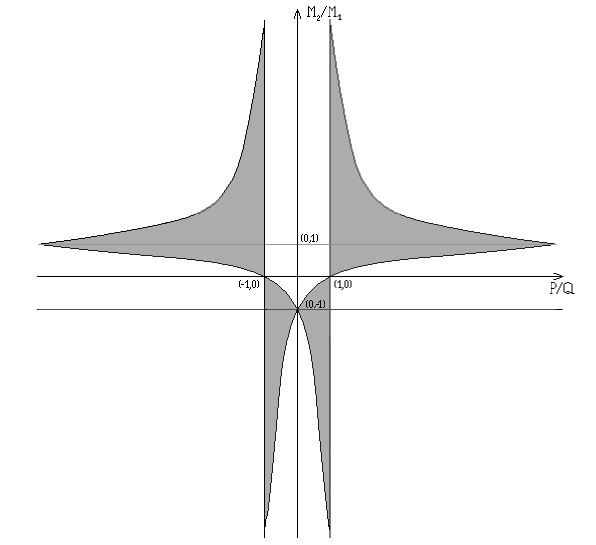
Figure 1: The grey zones denote the allowed regions for the ratio $M_{2}/M_{1}$ in terms of the ratio $P/Q$

Appendix B

The coefficients $c_{i}$, $1\leq i\leq 5$ that appear in equation (53) are

$$c_{1}=S^{2}\,z^{2}\,\frac{P_{2}(P_{1}^{2}-P_{2}^{2})(P_{1}z+P_{2})}{4(P_{1}+P_{2}z)^{2}},$$

$$c_{2}=-S^{2}\,z\,\frac{P_{2}(P_{1}^{2}-P_{2}^{2})[P_{1}(1+z^{2})+2\,P_{2}z]}{2(P_{1}+P_{2}z)^{2}},$$

$$c_{3}=\frac{(z-1)(P_{1}-P_{2})[Q_{1}z^{5}+Q_{2}z^{4}+Q_{3}z^{3}+Q_{4}z^{2}+Q_{5}z+Q_{6}]}{e_{2}(P_{1}-e_{1}\,e_{2})(P_{1}+P_{2}z)^{2}(P_{1}z+P_{2})^{2}z},$$

$$c_{4}=\frac{(z-1)^{2}(P_{1}-P_{2})(e_{2}^{2}-e_{1}\,e_{2}+P_{2})}{e_{2}(P_{2}z+P_{1})(P_{1}z+P_{2})},$$

$$c_{5}=\frac{(z-1)^{2}(P_{1}-P_{2})[R_{1}z^{4}+R_{2}z^{3}+R_{3}z+R_{4}]}{e_{2}(P_{1}+P_{2}z)^{2}(P_{1}z+P_{2})^{2}z},$$

with

$$\left\{\begin{array}[]{l}P_{1}=e_{1}(e_{2}-o_{1}),\\ P_{2}=o_{1}(e_{1}-e_{2}),\end{array}\right.$$ (86)

$$\left\{\begin{array}[]{l}Q_{1}=P_{1}\,P_{2}(P_{1}\,e_{1}+P_{2}\,e_{2}),\\ Q_{2}=P_{1}^{3}(e_{1}-e_{2})+P_{2}^{3}(e_{2}-o_{1})+P_{1}\,P_{2}(P_{2}\,e_{1}+2P_{1}\,e_{2}-P_{1}\,o_{1}),\\ Q_{3}=-P_{1}[P_{1}^{2}(e_{1}-e_{2})+P_{2}^{2}(e_{1}+4o_{1}-3\,e_{2})+P_{1}\,P_{2}(3e_{2}-e_{1})],\\ Q_{4}=-P_{2}[P_{1}^{2}(4e_{1}-3e_{2}+o_{1})+P_{2}^{2}(o_{1}-e_{2})+P_{1}\,P_{2}(3e_{2}-o_{1})],\\ Q_{5}=-P_{1}^{3}(e_{1}-e_{2})-P_{2}^{3}(e_{2}-o_{1})-P_{1}\,P_{2}(P_{2}\,e_{1}-2P_{1}\,e_{2}-P_{1}\,o_{1}),\\ Q_{6}=P_{1}\,P_{2}(P_{1}\,e_{2}+P_{2}\,o_{1}),\end{array}\right.$$ (93)

$$\left\{\begin{array}[]{l}R_{1}=P_{2}[P_{1}^{2}+P_{2}^{2}+P_{1}\,P_{2}+P_{2}(e_{2}^{2}-e_{1}\,e_{2})],\\ R_{2}=P_{2}^{3}+(e_{2}^{2}-e_{1}\,e_{2})(P_{2}^{2}-P_{1}^{2})+P_{1}\,P_{2}(e_{2}^{2}-e_{1}\,e_{2}+P_{1}+3P_{2}),\\ R_{3}=-P_{2}^{3}-(e_{2}^{2}-e_{1}\,e_{2})(P_{2}^{2}-P_{1}^{2})-P_{1}\,P_{2}(e_{2}^{2}-e_{1}\,e_{2}+P_{1}+P_{2}),\\ R_{4}=P_{1}(P_{1}\,e_{2}^{2}-P_{2}^{2}-P_{1}\,e_{1}\,e_{2}).\end{array}\right.$$ (98)

References

- [1] Ablowitz, M.J. and Ladik, J.K., “A nonlinear difference scheme and inverse scattering”, Stud. Appl. Math. 55, 213–229 (1976).
- [2] Abramowitz, M. and Stegun, I.A., Handbook of mathematical functions with formulas, graphs, and mathematical tables (Dover Publications, New York, 1992).
- [3] Calogero, F. and Eckhaus, W. , “Necessary conditions for integrability of nonlinear PDES”, Inverse Problems 3, L27–L32 (1987).
- [4] Degasperis, A. and Procesi, M., “Asymptotic integrability”, in Symmetry and perturbation theory (World Sci. Publishing, River Edge, NJ, 1999).
- [5] Hietarinta, J., “A new two–dimensional lattice model that is consistent around a cube”, Jour. Phys. A: Math. Gen. 37, L67–L73 (2004).
- [6] Jordan, C., Calculus of finite differences (Röttig and Romwalter, Sopron, 1939).
- [7] Leon, J. and Manna, M., “Multiscale analysis of discrete nonlinear evolution equations”, Jour. Phys. A: Math. Gen. 32, 2845–2869 (1999).
- [8] Levi, D., “Multiple–scale analysis of discrete nonlinear partial difference equations: the reduction of the lattice KdV”, Jour. Phys. A: Math. Gen. 38, 7677–7689 (2005).
- [9] Levi, D. and Heredero, H., “Multiscale analysis of discrete nonlinear evolution equations: the reduction of the dNLS”, Jour. Nonlinear Math. Phys. 12, suppl. 1, 440–448 (2005).
- [10] Nijhoff, F.W. and Capel, H.W., “The discrete Korteweg–de Vries equation”, Acta Appl. Math. 39, 133–158 (1995).
- [11] Taniuti, T., “Reductive perturbation method and far fields of wave equations”, Prog. Theor. Phys. 55 , 1–35 (1974).
- [12] Taniuti, T. and Nishihara, K., Nonlinear waves (Monographs and Studies in Mathematics, Pitman, Boston,1983).
- [13] Yamilov, R., “ Symmetries as integrability criteria for differential difference equations”, review article, in preparation.
- [14] Zhakarov, V.E. and Kuznetsov, E.A., “Multi–scale expansions in the theory of systems integrable by the inverse scattering transform”, Physica 18D, 455–463 (1986).