Riccati-parameter solutions of nonlinear second-order ODEs

Abstract

It has been proven by Rosu and Cornejo-Pérez [1, 2] that for some nonlinear second-order ODEs it is a very simple task to find one particular solution once the nonlinear equation is factorized with the use of two first-order differential operators. Here, it is shown that an interesting class of parametric solutions are easy to obtain if the proposed factorization has a particular form, which happily turns out to be the case in many problems of physical interest. The method that we exemplify with a few explicitly solved cases consists in using the general solution of the Riccati equation, which contributes with one parameter to this class of parametric solutions. For these nonlinear cases, the Riccati parameter serves as a ‘growth’ parameter from the trivial null solution up to the particular solution found through the factorization procedure.

PACS: 02.30.Jr, 02.30.Hq, 11.30.Pb

1 Introduction

Despite powerful integrability methods, such as the Lie group-theoretical approach, Painlevé analysis, existence of Lax representations and the associated inverse scattering transforms, the task of obtaining solutions of nonlinear second order partial and ordinary differential equations (ODEs) remains one of the most difficult problems in mathematical physics; in some cases, even finding one particular solution turns out to be a very difficult matter [3, 4]. However, in a number of cases, it has been proven that finding one particular solution turns out to be easier than expected. In the case of polynomial non-linearities, Rosu and Cornejo-Pérez [1, 2], working with a factorization procedure stemming from a work of Berkovich [5], have found that if the second order nonlinear differential equation can be factorized into two first order differential operators then it is easy to find a first particular solution for the problem. They considered a nonlinear equation of the type

$$\ddot{u}+g(u)\,\dot{u}+F(u)=0~{},$$ (1)

where the dots represent derivatives with respect to the independent variable $\tau$, which is usually the traveling coordinate of a reaction-diffusion equation [1]. The method they proposed was to factorize this equation in the following form

$$\left[D-\phi_{2}(u)\right]\left[D-\phi_{1}(u)\right]u=0~{},$$ (2)

(where $D\equiv\frac{d~{}}{d\tau}$) which implies the following conditions on the functions $\phi_{i}(u)$

$$-\left(\phi_{1}+\phi_{2}+\frac{d\phi_{1}}{du}\,u\right) = g(u)$$ (3)

$$\phi_{1}\,\phi_{2} = \frac{F(u)}{u}~{}.$$ (4)

If Eq. (1) can be factorized as in Eq. (2), then a first particular solution, say $u_{1}$, can be easily found by solving

$$\left[D-\phi_{1}(u)\right]u=0~{}.$$ (5)

2 Riccati-parameter solutions

Of course, obtaining one solution of a nonlinear second order ODE does not guarantee that one may find more general solutions. However, what Rosu and Cornejo-Pérez found was that in many cases (some of which will be described below) the function $\phi_{1}(u)$ turned out to be a linear function of the dependent variable $u$. Hence, Eq. (5) turns out to be a Riccati equation for this variable, which is very fortunate, since we already know how to find the general solution for this equation once a particular solution is known.

The appearance of the Riccati equation in linear second order differential equations is very common. In particular, it was very successfully exploited by Mielnik to find potentials which are isospectral to the simple harmonic oscillator potential [6], and it is a cornerstone for all SUSY developments [7]. However, it has not been used to solve nonlinear second-order differential equations at least in the way we present here.

Thus, if $\phi_{1}$ is of the form $\phi_{1}(u)=c_{1}u+c_{2}$, Eq. (5) transforms into the Riccati equation

$$\dot{u}-c_{1}u^{2}-c_{2}u=0$$ (6)

and if a particular solution $u_{1}$ of this equation is known, then the general solution can be found as [6]

$$u_{\lambda,c_{1}}=u_{1}+\frac{e^{I_{1}}}{\lambda-c_{1}\,I_{2}}~{},$$ (7)

where

$$I_{1}(\tau)\equiv\int_{\tau_{0}}^{\tau}(2c_{1}u_{1}(\tau^{\prime})+c_{2})d\tau^{\prime}$$ (8)

and

$$I_{2}(\tau)\equiv\int_{\tau_{0}}^{\tau}e^{I_{1}(\tau^{\prime})}d\tau^{\prime}\,.$$ (9)

Notice that for

$$\lambda_{s}=c_{1}I_{2}(\tau)~{},$$ (10)

a singularity may develop.

Eq. (7) provides in turn what we call as a Riccati-parameter solution of the nonlinear equation. We notice that the first parameter, $c_{1}$, is essentially the slope of the factorization function $\phi_{1}$, whereas the $\lambda$ parameter can be chosen in such a way as to prevent this solution from possessing singularities [6], although for nonlinear differential equations this is not an absolutely prohibitive issue. It will be seen in the examples given in the following that the latter parameter acts like a label in this class of solutions placing them between the trivial null solution and the particular solution given by Eq. (5).

3 Examples of physical interest

In this section we find the explicit form of the Riccati-parameter solution for three nonlinear equations of physical interest that are polynomial type Liénard equations, i.e., similar to Eq. (1) but with $F(u)$ a polynomial of order two and three in our cases.

3.1 Modified Emden equation

We start with the modified Emden equation

$$\ddot{u}+\alpha\,u\,\dot{u}+\beta\,u^{3}=0~{},$$ (11)

for which the first rigorous study has been done by Painlevé more than a century ago [8] who got solutions for $\beta=\alpha^{2}/9$ and $\beta=-\alpha^{2}$. Recently, Chandrasekar et al [9] provided a detailed discussion of this equation from the point of view of the modified Prelle-Singer procedure that gives the construction of the solution in terms of elementary functions if such a solution exists [10], although Iacono [11] noticed that much simpler connections with the Abel equation could be used to get the solutions. For the remarkable physical applications, see [9].

Employing $\phi_{1}=a_{1}\sqrt{\beta}\,u$ and $\phi_{2}=a_{1}^{-1}\sqrt{\beta}\,u$, where $a_{1}=-\frac{\alpha\pm\sqrt{\alpha^{2}-8\beta}}{4\sqrt{\beta}}$, one particular solution is [2]

$$u_{1}=-\frac{1}{a_{1}\sqrt{\beta}(\tau-\tau_{0})}~{}.$$ (12)

Hence, by using Eq. (7) one can find that the two-parameter solution of Eq. (11) is

$$u_{\lambda}=-\frac{1}{a_{1}\sqrt{\beta}(\tau-\tau_{0})}+\frac{1}{\lambda(\tau-\tau_{0})^{2}+a_{1}\sqrt{\beta}(\tau-\tau_{0})}~{}.$$ (13)

In this case it is instructive to notice that when $|\lambda|$ runs from zero to infinity, the $u_{\lambda}$ solution goes from the trivial solution $u=0$ to the particular solution $u=u_{1}$, as can be deduced from Eq. (13) and graphically seen in figure 1.

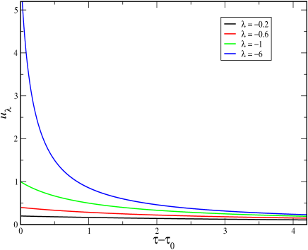
Fig. 1: $u_{\lambda}(\tau)$ in the case of the modified Emden equation for $\lambda=-0.2,-0.4,-1,-6$, from top to bottom respectively, and $a_{1}\sqrt{\beta}=-1$.

3.2 Convective Fisher equation

We pass now to the convective Fisher equation [12]

$$\ddot{u}+2(\nu-\mu\,u)\dot{u}+2u(1-u)=0~{}.$$ (14)

The second term corresponding to convection is introduced to describe mechanical transport in competition with diffusive transport or cases when external bias fields are present. In the context of population dynamics which is typical for the Fisher equation, it has been used by Walsh et al [13] to simulate the population mobility according to spatial gradients in the food supply.

Rosu and Cornejo-Pérez found that for $\nu=\mu/2+\mu^{-1}$, the factorization functions are $\phi_{1}=-\mu(1-u)$ and $\phi_{2}=-2/\mu$. Hence, a particular solution for this equation will be [2]

$$u_{1}=\left[1\pm\exp\left(\mu(\tau-\tau_{0})\right)\right]^{-1}~{}.$$ (15)

The $\lambda$-parameter solution can be readily obtained in the form

$$u_{\lambda}=u_{1}+\frac{e^{-\mu(\tau-\tau_{0})}}{\left[e^{-\mu(\tau-\tau_{0})}\pm 1\right]\left[\lambda\left(e^{-\mu(\tau-\tau_{0})}\pm 1\right)-1\right]}~{}.$$ (16)

Once again, $u_{0}=0$ and $u_{\infty}=u_{1}$. For the graphical representation see figure 2.

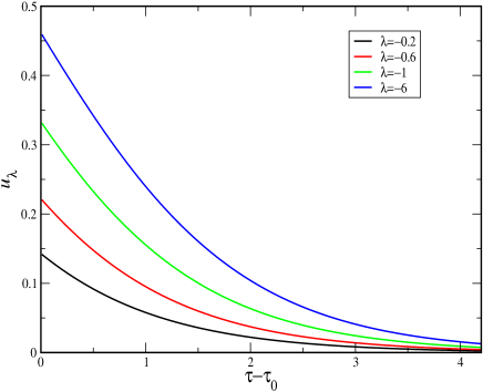
Fig. 2: Convective Fisher $u_{\lambda}(\tau)$ for $\lambda=-0.2,-0.4,-1,-6$, from top to bottom respectively, and $\mu=1$.

3.3 Generalized Liénard equation

Consider now the generalized Liénard equation for cubic nonlinear oscillators

$$\ddot{u}+g(u)\,\dot{u}+F_{3}=0~{},$$ (17)

where $F_{3}(u)=Au+Bu^{2}+Cu^{3}$. The previous equations can be seen as particular cases of this one. With $\Delta=\sqrt{B^{2}-4AC}$, Rosu and Cornejo-Pérez found that using

$$\phi_{1}=a_{1}\left(\frac{B+\Delta}{2}+Cu\right)\ \ ,\ \ \ \ \phi_{2}=a_{1}^{-1}\left(\frac{B-\Delta}{2C}+u\right)$$

for

$$g(u)=-\left[\frac{B+\Delta}{2}a_{1}+\frac{B-\Delta}{2C}a_{1}^{-1}+\left(2Ca_{1}+a_{1}^{-1}\right)u\right]$$ (18)

the following particular solution could be obtained [2]

$$u_{1}(\tau)=\frac{\frac{B+\Delta}{2}}{\exp\left(-a_{1}\frac{B+\Delta}{2}(\tau-\tau_{0})\right)-C}=\frac{\frac{B+\Delta}{2}\exp\left(a_{1}\frac{B+\Delta}{2}(\tau-\tau_{0})\right)}{1-C\exp\left(a_{1}\frac{B+\Delta}{2}(\tau-\tau_{0})\right)}~{}.$$ (19)

Now, using Eq. (7) and denoting $\xi=\tau-\tau_{0}$, we can see that the two-parameter solution in this case is

$$u_{\lambda}(\xi)=u_{1}+\frac{\frac{B+\Delta}{2}\exp\left(-a_{1}\frac{B+\Delta}{2}\xi\right)}{\left[\exp\left(-a_{1}\frac{B+\Delta}{2}\xi\right)-C\right]\left[\left(\lambda\frac{B+\Delta}{2}-1\right)\exp\left(-a_{1}\frac{B+\Delta}{2}\xi\right)-\lambda C\frac{B+\Delta}{2}\right]}~{}.$$ (20)

Varying $\lambda$ between 0 and $\infty$, the Riccati-parameter solutions go from the null solution to $u_{1}$. Plots of $u_{\lambda}$ for several values of $\lambda$ are displayed in figure 3.

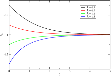
Fig. 3: Cubic Liénard $u_{\lambda}(\xi)$ solutions for $\lambda=0.7,0.9,1.1,1.3$, from top to bottom respectively, in the case $A=C=1$, $B=2$ ($\Delta=0$) and $a_{1}=1$.

3.4 Other cases of physical interest

The examples we have provided here are not the only possible cases that can be solved with this method, but they show the typical solutions to be found. Other examples where Riccati-parameter solutions can be obtained in this way are: the generalized Burgers-Huxley equation with $\delta=1,\ \gamma=1$, the generalized Fisher equation, with $n=2$, the Dixon-Tuszynski-Otwinowski type equation, with $n=4$, and the Fitzhugh-Nagumo equation [1]. The linear factorization functions $\phi_{1}$ of all these cases are given in [1]. Last but not least, we would like to comment on the possible physical interpretation of the Riccati parameter $\lambda$. We follow the works of Barton et al [14] and Monthus et al [15] to assert that $\lambda$ is related to the introduction of finite interval boundaries on the abscissa of the problem. This is very well described in Section II A of [15] to which the interested reader is directed. Essentially, the introduction of boundary conditions at certain points on the axis generates a modulation of the particular solution as presented here and the $\lambda$ parameter can be fixed through the boundary conditions. When the boundary is sent to infinity the original particular solution is recovered.

In conclusion, we introduced here an interesting class of parametric solutions of a number of physically relevant nonlinear differential equations. They cover the space between the null or constant solution and the particular solution obtained by a simple factorization method proposed previously.

We would like to thank Dr. O. Cornejo-Pérez for a careful reading of the first draft of this work. The second author wishes to thank CONACyT for partial support through project 46980.

References

- [1] Rosu H C and Cornejo-Pérez O 2005 Phys. Rev. E 71 046607, arXiv: math-ph/0401040.
- [2] Cornejo-Pérez O and Rosu H C 2005 Prog. Theor. Phys. 114 533, arXiv: math-ph/0504055.
- [3] Wang X Y 1988 Phys. Lett. A 131 277
- [4] Hereman W and Takaoka M 1990 J. Phys. A 23 4805
- [5] Berkovich L M 1992 Sov. Math. Dokl. 45 162
- [6] Mielnik B 1984 J. Math. Phys. 25 3387
- [7] For a review, see Cooper F, Khare A and Sukhatme U 1995 Phys. Rep. 251 267, arXiv: hep-th/9405029
- [8] Painlevé P 1902 Acta Math. 25 1
- [9] Chandrasekar V K, Senthilvelan M and Lakshmanan M 2007 J. Phys. A 40 4717
- [10] Chandrasekar V K, Senthilvelan M and Lakshmanan M 2005 Proc. Roy. Soc. Lond. A 461 2451, arXiv: nlin.SI/0408053.
- [11] Iacono R 2008 J. Phys. A 41 068001
- [12] Schönborn O, Desai R C and Stauffer D, 1994 J. Phys. A 27 L251, arXiv: cond-mat/9403025 Schönborn O, Puri S and Desai R C 1994 Phys. Rev. E 49 3480, arXiv: cond-mat/9312035
- [13] Walsh C, Ray T S and Jan N 1995 J. Stat. Phys. 81, 761
- [14] Barton G, Bray A J and McKane A J 1990 Am. J. Phys. 58, 751
- [15] Monthus C, Oshanin G, Comtet A and Burlatsky S F 1996 Phys. Rev. E 54 231