Stabilizing feedback controls for quantum systems

Abstract

No quantum measurement can give full information on the state of a quantum system; hence any quantum feedback control problem is neccessarily one with partial observations, and can generally be converted into a completely observed control problem for an appropriate quantum filter as in classical stochastic control theory. Here we study the properties of controlled quantum filtering equations as classical stochastic differential equations. We then develop methods, using a combination of geometric control and classical probabilistic techniques, for global feedback stabilization of a class of quantum filters around a particular eigenstate of the measurement operator.

1 Introduction

Though they are both probabilistic theories, probability theory and quantum mechanics have historically developed along very different lines. Nonetheless the two theories are remarkably close, and indeed a rigorous development of quantum probability [18] contains classical probability theory as a special case. The embedding of classical into quantum probability has a natural interpretation that is central to the idea of a quantum measurement: any set of commuting quantum observables can be represented as random variables on some probability space, and conversely any set of random variables can be encoded as commuting observables in a quantum model. The quantum probability model then describes the statistics of any set of measurements that we are allowed to make, whereas the sets of random variables obtained from commuting observables describe measurements that can be performed in a single realization of an experiment. As we are not allowed to make noncommuting observations in a single realization, any quantum measurement yields even in principle only partial information about the system.

The situation in quantum feedback control [10, 11] is thus very close to classical stochastic control with partial observations [3]. A typical quantum control scenario, representative of experiments in quantum optics, is shown in Fig. 1. We wish to control the state of a cloud of atoms, e.g. we could be interested in controlling their collective angular momentum. To observe the atoms, we scatter a laser probe field off the atoms and measure the scattered light using a homodyne detector (a cavity can be used to increase the interaction strength between the light and the atoms). The observation process is fed into a controller which can feed back a control signal to the atoms through some actuator, e.g. a time-varying magnetic field. The entire setup can be described by a Schrödinger equation for the atoms and the probe field, which takes the form of a “quantum stochastic differential equation” in a Markovian limit. The controller, however, only has access to the observations of the probe. The laser probe itself contributes quantum fluctuations to the observations, hence the observation process can be considered as a noisy observation of an atomic variable.

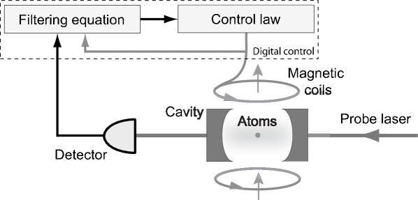
Fig. 1: A typical feedback control scenario in quantum optics. A probe laser scatters off a cloud of atoms in an optical cavity, and is ultimately detected. The detected signal is processed by a controller which feeds back to the system through a time varying magnetic field.

As in classical stochastic control we can use the properties of the conditional expectation to convert the output feedback control problem into one with complete observations. The conditional expectation $\pi_{t}(X)$ of an observable $X$ given the observations $\{Y_{s}:0\leq s\leq t\}$ is the least mean square estimate of $X_{t}$ (the observable $X$ at time $t$) given $Y_{s\leq t}$. One can obtain a quantum filtering equation [2, 4, 5] that propagates $\pi_{t}(X)$, or alternatively the conditional density matrix $\rho_{t}$ defined by the relation $\pi_{t}(X)={\rm Tr}[\rho_{t}X]$. This is the quantum counterpart of the classical Kushner-Stratonovich equation, due to Belavkin [2], and plays an equivalent role in quantum stochastic control. In particular, as $\mathbb{E}X_{t}=\mathbb{E}\pi_{t}(X)$ we can control the expectations of observables by designing a state feedback control law based on the filter.

Note that as the observation process $Y_{s\leq t}$ is measured in a single experimental realization, it is equivalent to a classical stochastic process (i.e. the observables $Y_{t}$ commute with each other at different times). But as the filter depends only on the observations, it is thus equivalent to a classical stochastic equation; in fact, the filter can be expressed as a classical (Itô) stochastic differential equation for the conditional density matrix $\rho_{t}$. Hence ultimately any quantum control problem of this form is reduced to a classical stochastic control problem for the filter.

In this paper we consider a class of quantum control problems of the following form. Rather than specifying a cost function to minimize, as in optimal control theory, we desire to asymptotically prepare a particular quantum state $\rho_{f}$ in the sense that $\mathbb{E}X_{t}\to{\rm Tr}[\rho_{f}X]$ as $t\to\infty$ for all $X$ (for a deterministic version see e.g. [21]). As $\mathbb{E}X_{t}=\mathbb{E}\pi_{t}(X)$, this comes down to finding a feedback control that will ensure the convergence $\rho_{t}\to\rho_{f}$ of the conditional density $\rho_{t}$. In addition to this convergence, we will show that our controllers also render the filter stochastically stable around the target state, which suggests some degree of robustness to perturbations. In §4 we will discuss the preparation of states in a cloud of atoms where the $z$-component of the angular momentum has zero variance, whereas in §5 we will discuss the preparation of correlated states of two spins. Despite their relatively simple description the creation of such states is not simple. Quantum feedback control may provide a desirable method to reliably prepare such states in practice (though other issues, e.g. the reduction of quantum filters [9] for efficient real-time implementation, must be resolved before such schemes can be realized experimentally; we refer to [7] for a state-of-the-art experimental demonstration of a related quantum control scenario.)

Though we have attempted to indicate the origin of the control problems studied here, a detailed treatment of either the physical or mathematical considerations behind our models is beyond the scope of this paper; for a rigorous introduction to quantum probability and filtering we refer to [5]. Instead we will consider the quantum filtering equation as our starting point, and investigate the classical stochastic control problem of feedback stabilization of this equation. In §2 we first introduce some tools from stochastic stability theory and stochastic analysis that we will use in our proofs. In §3 we introduce the quantum filtering equation and study issues such as existence and uniqueness of solutions, continuity of the paths, etc. In §4 we pose the problem of stabilizing an angular momentum eigenstate and prove global stability under a particular control law. It is our expectation that the methods of §4 are sufficiently flexible to be applied to a wide class of quantum state preparation scenarios. As an example, we use in §5 the techniques developed in §4 to stabilize particular entangled states of two spins. Additional results and numerical simulations will appear in [20].

2 Geometric tools for stochastic processes

In this section we briefly review two methods that will allow us to apply geometric control techniques to stochastic systems. The first is a stochastic version of the classical Lyapunov and LaSalle invariance theorems. The second, a support theorem for stochastic differential equations, will allow us to infer properties of stochastic sample paths through the study of a related deterministic system. We refer to the references for proofs of the theorems.

2.1 Lyapunov and LaSalle invariance theorems

The Lyapunov stability theory and LaSalle’s invariance theorem are important tools in the analysis of and control design for deterministic systems. Similarly, their stochastic counterparts will play an essential role in what follows. The subject of stochastic stability was studied extensively by Has’minskiĭ [12] and by Kushner [15]. We will cite a small selection of the results that will be needed in the following: a Lyapunov (local) stability theorem for Markov processes, and the LaSalle invariance theorem of Kushner [15, 16, 17].

Definition 1.

Let $x_{t}^{z}$ be a diffusion process on the metric state space $X$, started at $x_{0}=z$, and let $\tilde{z}$ denote an equilibrium position of the diffusion, i.e. $x_{t}^{\tilde{z}}=\tilde{z}$. Then

1. the equilibrium $\tilde{z}$ is said to be stable in probability if

   $$\lim_{z\to\tilde{z}}\mathbb{P}\left(\sup_{0\leq t<\infty}\|x_{t}^{z}-\tilde{z}\|\geq\varepsilon\right)=0\qquad\forall\varepsilon>0.$$ (1)

2. the equilibrium $\tilde{z}$ is globally stable if it is stable in probability and additionally

   $$\mathbb{P}\left(\lim_{t\to\infty}x_{t}^{z}=\tilde{z}\right)=1\qquad\forall z\in X.$$ (2)

In the following theorems we will make the following assumptions.

1. The state space $X$ is a complete separable metric space and $x_{t}^{z}$ is a homogeneous strong Markov process on $X$ with continuous sample paths.

2. $V(\cdot)$ is a nonnegative real-valued continuous function on $X$.

3. For $\lambda>0$, let $Q_{\lambda}=\{x\in X:V(x)<\lambda\}$ and assume $Q_{\lambda}$ is nonempty. Let $\tau_{\lambda}=\inf\{t:x_{t}^{z}\not\in Q_{\lambda}\}$ and define the stopped process $\tilde{x}_{t}^{z}=x^{z}_{t\wedge\tau_{\lambda}}$.

4. $\mathscr{A}_{\lambda}$ is the weak infinitesimal operator of $\tilde{x}_{t}$ and $V$ is in the domain of $\mathscr{A}_{\lambda}$.

The following theorems can be found in Kushner [15, 16, 17].

Theorem 2 (Local stability).

Let $\mathscr{A}_{\lambda}V\leq 0$ in $Q_{\lambda}$. Then the following hold:

1. $\lim_{t\to\infty}V(\tilde{x}_{t}^{z})$ exists a.s., so $V(x_{t}^{z})$ converges for a.e. path remaining in $Q_{\lambda}$.

2. $\mathbb{P}\mbox{\rm-lim}_{t\to\infty}\mathscr{A}_{\lambda}V(\tilde{x}_{t}^{z})=0$, so $\mathscr{A}_{\lambda}V(x_{t}^{z})\to 0$ in probability as $t\to\infty$ for almost all paths which never leave $Q_{\lambda}$.

3. For $z\in Q_{\lambda}$ and $\alpha\leq\lambda$ we have the uniform estimate

   $$\mathbb{P}\left(\sup_{0\leq t<\infty}V(x_{t}^{z})\geq\alpha\right)=\mathbb{P}\left(\sup_{0\leq t<\infty}V(\tilde{x}_{t}^{z})\geq\alpha\right)\leq\frac{V(z)}{\alpha}.$$ (3)

4. If $V(\tilde{z})=0$ and $V(x)\neq 0$ for $x\neq\tilde{z}$, then $\tilde{z}$ in stable in probability.

The following theorem is a stochastic version of the LaSalle invariance theorem. Recall that a diffusion $x_{t}^{z}$ is said to be Feller continuous if for fixed $t$, $\mathbb{E}G(x_{t}^{z})$ is continuous in $z$ for any bounded continuous $G$.

Theorem 3 (Invariance).

Let $\mathscr{A}_{\lambda}V\leq 0$ in $Q_{\lambda}$. Suppose $Q_{\lambda}$ has compact closure, $\tilde{x}_{t}^{z}$ is Feller continuous, and that $\mathbb{P}(\|\tilde{x}_{t}^{z}-z\|>\varepsilon)\to 0$ as $t\to 0$ for any $\varepsilon>0$, uniformly for $z\in Q_{\lambda}$. Then $\tilde{x}_{t}^{z}$ converges in probability to the largest invariant set contained in $C_{\lambda}=\{x\in Q_{\lambda}:\mathscr{A}_{\lambda}V(x)=0\}$. Hence $x_{t}^{z}$ converges in probability to the largest invariant set contained in $C_{\lambda}$ for almost all paths which never leave $Q_{\lambda}$.

2.2 The support theorem

In the nonlinear control of deterministic systems an important role is played by the application of geometric methods, e.g. Lie algebra techniques, to the vector fields generating the control system. Such methods can usually not be directly applied to stochastic systems, however, as the processes involved are not (sufficiently) differentiable. The support theorem for stochastic differential equations, in its original form due to Stroock and Varadhan [24], connects events of probability one for a stochastic differential equation to the solution properties of an associated deterministic system. One can then apply classical techniques to the latter and invoke the support theorem to apply the results to the stochastic system; see e.g. [13] for the application of Lie algebraic methods to stochastic systems.

We quote the following form of the theorem [14, 13].

Theorem 4.

Let $M$ be a connected, paracompact $C^{\infty}$-manifold and let $X_{k}$, $k=0\ldots n$ be $C^{\infty}$ vector fields on $M$ such that all linear sums of $X_{k}$ are complete. Let $X_{k}=\sum_{l}X_{k}^{l}(x)\partial_{l}$ in local coordinates and consider the Stratonovich equation

$$dx_{t}=X_{0}(x_{t})\,dt+\sum_{k=1}^{n}X_{k}(x_{t})\circ dW_{t}^{k},\qquad x_{0}=x.$$ (4)

Consider in addition the associated deterministic control system

$$\frac{d}{dt}x_{t}^{u}=X_{0}(x_{t}^{u})+\sum_{k=1}^{n}X_{k}(x_{t}^{u})u^{k}(t),\qquad x_{0}^{u}=x$$ (5)

with $u^{k}\in\mathscr{U}$, the set of all piecewise constant functions from $\mathbb{R}_{+}$ to $\mathbb{R}$. Then

$$\mathscr{S}_{x}=\overline{\{x^{u}_{\cdot}:u\in\mathscr{U}^{n}\}}\subset\mathscr{W}_{x}$$ (6)

where $\mathscr{W}_{x}$ is the set of all continuous paths from $\mathbb{R}_{+}$ to $M$ starting at $x$, equipped with the topology of uniform convergence on compact sets, and $\mathscr{S}_{x}$ is the smallest closed subset of $\mathscr{W}_{x}$ such that $\mathbb{P}(\{\omega\in\Omega:x_{\cdot}(\omega)\in\mathscr{S}_{x}\})=1$.

3 Solution properties of quantum filters

The purpose of this section is to introduce the dynamical equations for a general quantum system with feedback and to establish their basic solution properties.

We will consider quantum systems with finite dimension $1<N<\infty$. The state space of such a system is given by the set of density matrices

$$\mathcal{S}=\{\rho\in\mathbb{C}^{N\times N}:\rho=\rho^{*},~{}{\rm Tr}\,\rho=1,~{}\rho\geq 0\}$$ (7)

where $\rho^{*}$ denotes Hermitian conjugation. In noncommutative probability the space $\mathcal{P}$ is the analog of the set of probability measures of an $N$-state random variable. Finite-dimensional quantum systems are ubiquitous in contemporary quantum physics; a system with dimension $N=2^{n}$, for example, can represent the collective state of $n$ qubits in the setting of quantum computing, and $N=2J+1$ represents a system with fixed angular momentum $J$. The following lemma describes the structure of $\mathcal{S}$:

Lemma 5.

$\mathcal{S}$ is the convex hull of $\{\rho\in\mathbb{C}^{N\times N}:\rho=vv^{*},~{}v\in\mathbb{C}^{N},~{}v^{*}v=1\}$.

Proof.

The statement is easily verified by diagonalizing the elements of $\mathcal{P}$.   ∎

We now consider continuous measurement of such a system, e.g. by weakly coupling it to an optical probe field and performing a diffusive observation of the field. When the state of the system is conditioned on the observation process we obtain the following matrix-valued Itô equation for the conditional density, which is a quantum analog of the Kushner-Stratonovich equation of nonlinear filtering [2, 4, 10]:

$$\begin{split}d\rho_{t}=-i(H_{t}\rho_{t}-\rho_{t}H_{t})\,dt+(c\rho_{t}&c^{*}-\tfrac{1}{2}(c^{*}c\rho_{t}+\rho_{t}c^{*}c))\,dt\\ &+\sqrt{\eta}\,(c\rho_{t}+\rho_{t}c^{*}-{\rm Tr}[(c+c^{*})\rho_{t}]\rho_{t})\,dW_{t}.\end{split}$$ (8)

Here we have introduced the following quantities:

• The Wiener process $W_{t}$ is the innovation $dW_{t}=dy_{t}-\sqrt{\eta}\,{\rm Tr}[(c+c^{*})\rho_{t}]dt$. Here $y_{t}$, a continuous semimartingale with quadratic variation $\langle y,y\rangle_{t}=t$, is the observation process obtained from the system.

• $H_{t}=H_{t}^{*}$ is a Hamiltonian matrix which describes the action of external forces on the system. We will consider $H_{t}$ of the form $H_{t}=F+u_{t}G$ with $F=F^{*}$, $G=G^{*}$ and the (real) scalar control input $u_{t}$.

• $u_{t}$ is a bounded real càdlàg process that is adapted to $\mathcal{F}_{t}^{y}=\sigma(y_{s},0\leq s\leq t)$, the filtration generated by the observations up to time $t$.

• $c$ is a matrix which determines the coupling to the external (readout) field.

• $0<\eta\leq 1$ is the detector efficiency.

Let us begin by studying a different form of the equation (8). Consider the linear Itô equation

$$d\tilde{\rho}_{t}=-i(H_{t}\tilde{\rho}_{t}-\tilde{\rho}_{t}H_{t})\,dt+(c\tilde{\rho}_{t}c^{*}-\tfrac{1}{2}(c^{*}c\tilde{\rho}_{t}+\tilde{\rho}_{t}c^{*}c))\,dt+\sqrt{\eta}\,(c\tilde{\rho}_{t}+\tilde{\rho}_{t}c^{*})\,dy_{t},$$ (9)

which is the quantum analog of the Zakai equation. As it obeys a global (random) Lipschitz condition, this equation has a unique strong solution ([23], pp. 249–253).

Lemma 6.

The set of nonnegative nonzero matrices is a.s. invariant for (9).

Proof.

We begin by expanding $\tilde{\rho}_{0}$ into its eigenstates, i.e. $\tilde{\rho}_{0}=\sum_{i}\lambda_{i}v_{0}^{i}v_{0}^{i*}$ with $v_{0}^{i}\in\mathbb{C}^{N}$ being the $i$th eigenvector and $\lambda_{i}$ the $i$th eigenvalue. As $\tilde{\rho}_{0}$ is nonnegative all the $\lambda_{i}$ are nonnegative. Now consider the set of equations

$$d\rho_{t}^{i}=-i(H_{t}\rho_{t}^{i}-\rho_{t}^{i}H_{t})\,dt+(c\rho_{t}^{i}c^{*}-\tfrac{1}{2}(c^{*}c\rho_{t}^{i}+\rho_{t}^{i}c^{*}c))\,dt+(c\rho_{t}^{i}+\rho_{t}^{i}c^{*})\,dW_{t}^{\prime}$$ (10)

with $\rho_{0}^{i}=v_{0}^{i}v_{0}^{i*}$. Here we have extended our probability space to admit a Wiener process $\hat{W}_{t}$ that is independent of $y_{t}$, and $W^{\prime}_{t}=\sqrt{\eta}\,y_{t}+\sqrt{1-\eta}\,\hat{W}_{t}$. The process $\tilde{\rho}_{t}$ is then equivalent in law to $\mathbb{E}[\rho_{t}^{\prime}|\mathcal{F}_{t}^{y}]$, where $\rho_{t}^{\prime}=\sum_{i}\lambda_{i}\rho_{t}^{i}$.

Now note that the solution of the set of equations

$$dv_{t}^{i}=-iH_{t}v_{t}^{i}\,dt-\tfrac{1}{2}c^{*}c\,v_{t}^{i}\,dt+c\,v_{t}^{i}\,dW_{t}^{\prime},~{}~{}~{}~{}~{}~{}~{}~{}~{}~{}~{}~{}~{}~{}v_{t}^{i}\in\mathbb{C}^{N}$$ (11)

satisfies $\rho_{t}^{i}=v_{t}^{i}v_{t}^{i*}$, as is readily verified by Itô’s rule. By [23], pp. 326 we have that $v_{t}^{i}=U_{t}v_{0}^{i}$ where the random matrix $U_{t}$ is a.s. invertible for all $t$. Hence a.s. $v_{t}^{i}\neq 0$ for any finite time unless $v_{0}^{i}=0$. Thus clearly $\rho_{t}^{\prime}$ is a.s. a nonnegative nonzero matrix for all $t$, and the result follows.   ∎

Proposition 7.

Eq. (8) has a unique strong solution $\rho_{t}=\tilde{\rho}_{t}/{\rm Tr}\,\tilde{\rho}_{t}$ in $\mathcal{S}$.

Clearly this must be satisfied if (8) is to propagate a density.

Proof.

As the set of nonnegative nonzero matrices is invariant for $\tilde{\rho}_{t}$, this implies in particular that ${\rm Tr}\,\tilde{\rho}_{t}>0$ for all $t$ a.s. Thus the result follows simply from application of Itô’s rule to (9), and from the fact that if $M=\sum_{i}\lambda_{i}v_{i}$ is a nonnegative nonzero matrix, then $M/{\rm Tr}\,M=\sum_{i}(\lambda_{i}/\sum_{j}\lambda_{j})v_{i}\in\mathcal{S}$.   ∎

Proposition 8.

The following uniform estimate holds for (8):

$$\mathbb{P}\left(\sup_{0\leq\delta\leq\Delta}\|\rho_{t+\delta}-\rho_{t}\|>\varepsilon\right)\leq C\Delta(1+\Delta)\qquad\forall\varepsilon>0$$ (12)

where $0<C<\infty$ depends only on $\varepsilon$ and $\|\cdot\|$ is the Frobenius norm. Hence the solution of (8) is stochastically continuous uniformly in $t$ and $\rho_{0}$.

Proof.

Write $\rho_{t}=\rho_{0}+\Phi_{t}+\Xi_{t}$ where

$$\Phi_{t}=\int_{0}^{t}\left[-i(H_{s}\rho_{s}-\rho_{s}H_{s})+(c\rho_{s}c^{*}-\tfrac{1}{2}(c^{*}c\rho_{s}+\rho_{s}c^{*}c))\right]ds,$$ (13)

$$\Xi_{t}=\int_{0}^{t}\sqrt{\eta}\,(c\rho_{s}+\rho_{s}c^{*}-{\rm Tr}[(c+c^{*})\rho_{s}]\rho_{s})\,dW_{s}.$$ (14)

For $\Xi_{t}$ we have the estimate ([1], pp. 81)

$$\mathbb{E}\left(\sup_{0\leq\delta\leq\Delta}\|\Xi_{t+\delta}-\Xi_{t}\|^{2}\right)\leq 4\eta\int_{t}^{t+\Delta}\mathbb{E}\|c\rho_{s}+\rho_{s}c^{*}-{\rm Tr}[(c+c^{*})\rho_{s}]\rho_{s}\|^{2}\,ds.$$ (15)

As the integrand is bounded clearly this expression is bounded by $C_{1}\Delta$ for some positive constant $C_{1}<\infty$. For $\Phi_{t}$ we can write

$$\mathbb{E}\left(\sup_{0\leq\delta\leq\Delta}\|\Phi_{t+\delta}-\Phi_{t}\|^{2}\right)\leq\mathbb{E}\left[\sup_{0\leq\delta\leq\Delta}\int_{t}^{t+\delta}\|G_{s}\|\,ds\right]^{2}=\mathbb{E}\left[\int_{t}^{t+\Delta}\|G_{s}\|\,ds\right]^{2}$$ (16)

where $G_{s}$ denotes the integrand of (13). As $\|G_{s}\|$ is bounded we can estimate this expression by $C_{2}\Delta^{2}$ with $C_{2}<\infty$. Using $\|A+B\|^{2}\leq 2(\|A\|^{2}+\|B\|^{2})$ we can write

$$\sup_{0\leq\delta\leq\Delta}\|\rho_{t+\delta}-\rho_{t}\|^{2}\leq 2\left(\sup_{0\leq\delta\leq\Delta}\|\Phi_{t+\delta}-\Phi_{t}\|^{2}+\sup_{0\leq\delta\leq\Delta}\|\Xi_{t+\delta}-\Xi_{t}\|^{2}\right).$$ (17)

Finally, Chebychev’s inequality gives

$$\mathbb{P}\left(\sup_{0\leq\delta\leq\Delta}\|\rho_{t+\delta}-\rho_{t}\|>\varepsilon\right)\leq\frac{1}{\varepsilon^{2}}\mathbb{E}\left(\sup_{0\leq\delta\leq\Delta}\|\rho_{t+\delta}-\rho_{t}\|^{2}\right)\leq\frac{2C_{1}\Delta+2C_{2}\Delta^{2}}{\varepsilon^{2}}$$ (18)

from which the result follows.   ∎

Remark. The statistics of the observation process $y_{t}$ should of course depend both on the control $u_{t}$ that is applied to the system and on the initial state $\rho_{0}$. We will always assume that the filter initial state $\rho_{0}$ matches the state in which the system is initially prepared (i.e. we do not consider “wrongly initialized” filters) and that the same control $u_{t}$ is applied to the system and to the filter (see Fig. 1). Quantum filtering theory then guarantees that the innovation $W_{t}$ is a Wiener process. To simplify our proofs, we make from this point on the following choice: for all initial states and control policies, the corresponding observation processes are defined in such a way that they give rise to the same innovation process $W_{t}$.

We now specialize to the following case:

• $u_{t}=u(\rho_{t})$ with $u\in C^{1}(\mathcal{S},\mathbb{R})$.

In this simple feedback case we can prove several important properties of the solutions. First, however, we must show existence and uniqueness for the filtering equation with feedback: it is not a priori obvious that the feedback $u_{t}=u(\rho_{t})$ results in a well-defined càdlàg control.

Proposition 9.

Eq. (8) with $u_{t}=u(\rho_{t})$, $u\in C^{1}$ and $\rho_{0}=\rho\in\mathcal{S}$ has a unique strong solution $\rho_{t}\equiv\varphi_{t}(\rho,u)$ in $\mathcal{S}$, and $u_{t}$ is a continuous bounded control.

Proof.

As $\mathcal{S}$ is compact, we can find an open set $\mathcal{T}\subset\mathbb{C}^{N\times N}$ such that $\mathcal{S}$ is strictly contained in $\mathcal{T}$. Let $C(\rho):\mathbb{C}^{N\times N}\to[0,1]$ be a smooth function with compact support such that $C(\rho)=1$ for $\rho\in\mathcal{T}$, and let $U(\rho)$ be a $C^{1}(\mathbb{C}^{N\times N},\mathbb{R})$ function such that $U(\rho)=u(\rho)$ for $\rho\in\mathcal{S}$. Then the equation

$$d\bar{\rho}_{t}=-iC(\bar{\rho}_{t})[F+U(\bar{\rho}_{t})G,\bar{\rho}_{t}]\,dt+C(\bar{\rho}_{t})(c\bar{\rho}_{t}c^{*}-\tfrac{1}{2}(c^{*}c\bar{\rho}_{t}+\bar{\rho}_{t}c^{*}c))\,dt\\ +C(\bar{\rho}_{t})\sqrt{\eta}\,(c\bar{\rho}_{t}+\bar{\rho}_{t}c^{*}-{\rm Tr}[(c+c^{*})\bar{\rho}_{t}]\bar{\rho}_{t})\,dW_{t},$$

where $[A,B]=AB-BA$, has global Lipschitz coefficients and hence has a unique strong solution in $\mathbb{C}^{N\times N}$ and a.s. continuous adapted sample paths [23]. Moreover $\bar{\rho}_{t}$ must be bounded as $C(\rho)$ has compact support. Hence $U_{t}=U(\bar{\rho}_{t})$ is an a.s. continuous, bounded adapted process.

Now consider the solution $\rho_{t}$ of (8) with $u_{t}=U(\bar{\rho}_{t})$ and $\rho_{0}=\bar{\rho}_{0}\in\mathcal{S}$. As both $\rho_{t}$ and $\bar{\rho}_{t}$ have a unique solution, the solutions must coincide up to the first exit time from $\mathcal{T}$. But we have already established that $\rho_{t}$ remains in $\mathcal{S}$ for all $t>0$, so $\bar{\rho}_{t}$ can certainly never exit $\mathcal{T}$. Hence $\bar{\rho}_{t}=\rho_{t}$ for all $t>0$, and the result follows.   ∎

In the following, we will denote by $\varphi_{t}(\rho,u)$ the solution of (8) at time $t$ with the control $u_{t}=u(\rho_{t})$ and initial condition $\rho_{0}=\rho\in\mathcal{S}$.

Proposition 10.

If $V(\rho)$ is continuous, then $\mathbb{E}V(\varphi_{t}(\rho,u))$ is continuous in $\rho$; i.e., the diffusion (8) is Feller continuous.

Proof.

Let $\{\rho^{n}\in\mathcal{S}\}$ be a sequence of points converging to $\rho^{\infty}\in\mathcal{S}$. Let us write $\rho^{n}_{t}=\varphi_{t}(\rho^{n},u)$ and $\rho^{\infty}_{t}=\varphi_{t}(\rho^{\infty},u)$. First, we will show that

$${\mathbb{E}}\|\rho^{n}_{t}-\rho^{\infty}_{t}\|^{2}\rightarrow 0\quad\mbox{as}\quad n\rightarrow\infty.$$ (19)

where $\|\cdot\|$ is the Frobenius norm ($\|A\|^{2}=(A,A)$ with the inner product $(A,B)=\mathrm{Tr}\left(A^{*}B\right)$). We will write $\delta_{t}^{n}=\rho^{n}_{t}-\rho^{\infty}_{t}$. Using Itô’s rule we obtain

$$\begin{split}{\mathbb{E}}\|\delta_{t}^{n}&\|^{2}=\|\delta_{0}^{n}\|^{2}+\int_{0}^{t}\eta{\mathbb{E}}\mathrm{Tr}\left((c\delta_{s}^{n}+\delta_{s}^{n}c^{*}-{\rm Tr}[(c+c^{*})\rho_{s}^{n}]\rho_{s}^{n}+{\rm Tr}[(c+c^{*})\rho_{s}^{\infty}]\rho_{s}^{\infty})^{2}\right)ds\\ &+\int_{0}^{t}2\,{\mathbb{E}}\left[\mathrm{Tr}\left((i[\rho_{s}^{n},H(\rho_{s}^{n})]-i[\rho_{s}^{\infty},H(\rho_{s}^{\infty})])\delta_{s}^{n}\right)+\mathrm{Tr}\left(c\delta_{s}^{n}c^{*}\delta_{s}^{n}-c^{*}c(\delta_{s}^{n})^{2}\right)\right]ds\end{split}$$ (20)

where $[A,B]=AB-BA$. Let us estimate each of these terms. We have

$$\begin{split}\mathrm{Tr}\left(c^{*}c(\delta_{t}^{n})^{2}\right)&=\|c\delta_{t}^{n}\|^{2}\leq C_{1}\|\delta_{t}^{n}\|^{2}\\ \mathrm{Tr}\left(c\delta_{t}^{n}c^{*}\delta_{t}^{n}\right)&=(\delta_{t}^{n}c,c\delta_{t}^{n})\leq\|\delta_{t}^{n}c\|~{}\|c\delta_{t}^{n}\|\leq C_{2}\|\delta_{t}^{n}\|^{2}\end{split}$$ (21)

where we have used the Cauchy-Schwartz inequality and the fact that all the operators are bounded. Next we tackle

$$\mathrm{Tr}\left((i[\rho_{t}^{n},H(\rho_{t}^{n})]-i[\rho_{t}^{\infty},H(\rho_{t}^{\infty})])\delta_{t}^{n}\right)\leq\|i[\rho_{t}^{n},H(\rho_{t}^{n})]-i[\rho_{t}^{\infty},H(\rho_{t}^{\infty})]\|~{}\|\delta_{t}^{n}\|.$$ (22)

Now note that $S(\rho)=i[\rho,H(\rho)]=i[\rho,F+u(\rho)G]$ is $C^{1}$ in the matrix elements of $\rho$, and its derivatives are bounded as $\mathcal{S}$ is compact. Hence $S(\rho)$ is Lipschitz continuous, and we have

$$\|S(\rho_{t}^{n})-S(\rho_{t}^{\infty})\|\leq C_{3}\|\rho_{t}^{n}-\rho_{t}^{\infty}\|=C_{3}\|\delta_{t}^{n}\|$$ (23)

which implies

$$\mathrm{Tr}\left((i[\rho_{t}^{n},H(\rho_{t}^{n})]-i[\rho_{t}^{\infty},H(\rho_{t}^{\infty})])\delta_{t}^{n}\right)\leq C_{3}\|\delta_{t}^{n}\|^{2}.$$ (24)

Finally, we have $\|c\delta_{t}^{n}+\delta_{t}^{n}c^{*}\|\leq C_{4}\|\delta_{t}^{n}\|$ due to boundedness of multiplication with $c$, and a similar Lipschitz argument as the one above can be applied to $S^{\prime}(\rho)={\rm Tr}[(c+c^{*})\rho]\rho$, giving

$$\|{\rm Tr}[(c+c^{*})\rho_{t}^{n}]\rho_{t}^{n}-{\rm Tr}[(c+c^{*})\rho_{t}^{\infty}]\rho_{t}^{\infty}\|\leq C_{5}\|\delta_{t}^{n}\|.$$ (25)

We can now use $\|A+B\|^{2}\leq\|A\|^{2}+2\|A\|\,\|B\|+\|B\|^{2}$ to estimate the last term in (20) by $C_{6}\|\delta_{t}^{n}\|^{2}$. Putting all these together, we obtain

$${\mathbb{E}}\|\delta_{t}^{n}\|^{2}\leq\|\delta_{0}^{n}\|^{2}+C\int_{0}^{t}{\mathbb{E}}\|\delta_{s}^{n}\|^{2}ds$$ (26)

and thus by Gronwall’s lemma

$${\mathbb{E}}\|\delta_{t}^{n}\|^{2}\leq e^{Ct}\|\delta_{0}^{n}\|^{2}=e^{Ct}\|\rho^{n}-\rho^{\infty}\|^{2}.$$ (27)

As $t$ is fixed, Eq. (19) follows.

We have now proved that $\rho_{t}^{n}\to\rho_{t}^{\infty}$ in mean square as $n\to\infty$, which implies convergence in probability. But then for any continuous $V$, $V(\rho_{t}^{n})\to V(\rho_{t}^{\infty})$ in probability ([8], pp. 60). As $\mathcal{S}$ is compact, $V$ is bounded and we have

$$\mathbb{E}V(\rho_{t}^{\infty})=\mathbb{E}[\mathop{\mathbb{P}\mbox{-lim}}_{n\to\infty}V(\rho_{t}^{n})]=\lim_{n\to\infty}\mathbb{E}V(\rho_{t}^{n})$$ (28)

by dominated convergence ([8], pp. 72). But as this holds for any convergent sequence $\rho^{n}$, the result follows.   ∎

Proposition 11.

$\varphi_{t}(\rho,u)$ is a strong Markov process in $\mathcal{S}$.

Proof.

The proof of the Markov property in [22], pp. 109–110, carries over to our case. But then the strong Markov property follows from Feller continuity [15].   ∎

Proposition 12.

Let $\tau$ be the first exit time of $\rho_{t}$ from an open set $Q\subset\mathcal{S}$ and consider the stopped process $\rho_{t}^{Q}=\varphi_{t\wedge\tau}(\rho,u)$. Then $\rho_{t}^{Q}$ is also a strong Markov process in $\mathcal{S}$. Furthermore, for $V$ s.t. $\mathscr{A}V$ exists and is continuous, where $\mathscr{A}$ is the weak infinitesimal operator associated to $\varphi_{t}(\rho,u)$, we have $\mathscr{A}_{Q}V(x)=\mathscr{A}V(x)$ if $x\in Q$ and $\mathscr{A}_{Q}V(x)=0$ if $x\neq Q$ for the weak infinitesimal operator $\mathscr{A}_{Q}$ associated to $\rho_{t}^{Q}$.

Proof.

This follows from [15], pp. 11–12, and Proposition 8.   ∎

4 Angular momentum systems

In this section we consider a quantum system with fixed angular momentum $J$ ($2J\in\mathbb{N}$), e.g. an atomic ensemble, which is detected through a dispersive optical probe [11]. After conditioning, such systems are described by an equation of the form (8) where

• The Hilbert space dimension $N=2J+1$;

• $c=\beta F_{z}$, $F=0$ and $G=\gamma F_{y}$ with $\beta,\gamma>0$.

Here $F_{y}$ and $F_{z}$ are the (self-adjoint) angular momentum operators defined as follows. Let $\{\psi_{k}:k=0\ldots 2J\}$ be the standard basis in $\mathbb{C}^{N}$, i.e. $\psi_{i}$ is the vector with a single nonzero element $\psi_{i}^{i}=1$. Then [19]

$$\begin{split}F_{y}\psi_{k}&=ic_{k-J}\psi_{k+1}-ic_{J-k}\psi_{k-1},\\ F_{z}\psi_{k}&=(k-J)\psi_{k}\end{split}$$ (29)

with $c_{m}=\tfrac{1}{2}\sqrt{(J-m)(J+m+1)}$. Without loss of generality we will choose $\beta=\gamma=1$, as we can always rescale time and $u_{t}$ to obtain any $\beta,\gamma$.

Let us begin by studying the dynamical behavior of the resulting equation,

$$d\rho_{t}=-iu_{t}[F_{y},\rho_{t}]\,dt-\tfrac{1}{2}[F_{z},[F_{z},\rho_{t}]]\,dt+\sqrt{\eta}\,(F_{z}\rho_{t}+\rho_{t}F_{z}-2\,{\rm Tr}[F_{z}\rho_{t}]\rho_{t})\,dW_{t}$$ (30)

without feedback $u_{t}=0$.

Proposition 13 (Quantum state reduction).

For any $\rho_{0}\in\mathcal{S}$, the solution $\rho_{t}$ of (30) with $u_{t}=0$ converges a.s. as $t\to\infty$ to one of $\psi_{m}\psi_{m}^{*}$.

Proof.

We will apply Theorem 2 with $Q_{\lambda}=\mathcal{S}$. Consider the Lyapunov function $v(\rho)=\mbox{Tr}[F_{z}^{2}\rho]-(\mbox{Tr}[F_{z}\rho])^{2}$. One easily calculates $\mathscr{A}v(\rho)=-4\eta\,v(\rho)^{2}\leq 0$ and hence

$$\mathbb{E}v(\rho_{t})=v(\rho_{0})-4\eta\int_{0}^{t}\mathbb{E}v(\rho_{s})^{2}\,ds$$ (31)

by using the Itô rules. Note that $v(\rho)\geq 0$, so

$$4\eta\int_{0}^{t}\mathbb{E}v(\rho_{s})^{2}\,ds=v(\rho_{0})-\mathbb{E}v(\rho_{t})\leq v(\rho_{0})<\infty.$$ (32)

Thus we have by monotone convergence

$$\mathbb{E}\int_{0}^{\infty}v(\rho_{s})^{2}\,ds<\infty\quad\Longrightarrow\quad\int_{0}^{\infty}v(\rho_{s})^{2}\,ds<\infty\quad\mbox{a.s.}$$ (33)

By Theorem 2 the limit of $v(\rho_{t})$ as $t\to\infty$ exists a.s., and hence Eq. (33) implies that $v(\rho_{t})\to 0$ a.s. But the only states $\rho$ that satisfy $v(\rho)=0$ are $\rho=\psi_{m}\psi_{m}^{*}$.   ∎

The main goal of this section is to provide a feedback control law that globally stabilizes (30) around the equilibrium solution $(\rho_{t}\equiv\rho_{f},u\equiv 0)$, where we select a target state $\rho_{f}=v_{f}v_{f}^{*}$ from one of $v_{f}=\psi_{m}$.

Stabilization of quantum state reduction for low-dimensional angular momentum systems has been studied in [10]. It is shown that the main challenge in such a stabilization problem is due to the geometric symmetry hidden in the state space of the system. Many natural feedback laws fail to stabilize the closed-loop system around the equilibrium point $\rho_{f}$ because of this symmetry: the $\omega$-limit set contains points other than $\rho_{f}$. The approach of [10] uses computer searches to find continuous control laws that break this symmetry and globally stabilize the desired state. Unfortunately, the method is computationally involved and can only be applied to low-dimensional systems. Additionally, it is difficult to prove stability in this way for arbitrary parameter values, as the method is not analytical.

Here we present a different approach which avoids the unwanted limit points by changing the feedback law around them. The approach is entirely analytical and globally stabilizes the desired target state for any dimension $N$ and $0<\eta\leq 1$. The main result of this section can be stated as follows:

Theorem 14.

Consider the system (30) evolving in the set ${\mathcal{S}}$. Let $\rho_{f}=v_{f}v_{f}^{*}$ where $v_{f}$ is one of $\psi_{m}$, and let $\gamma>0$. Consider the following control law:

1. $u_{t}=-\mathrm{Tr}\left(i[F_{y},\rho_{t}]\rho_{f}\right)$ if $\mathrm{Tr}\left(\rho_{t}\rho_{f}\right)\geq\gamma$;

2. $u_{t}=1$ if $\mathrm{Tr}\left(\rho_{t}\rho_{f}\right)\leq\gamma/2$;

3. If $\rho_{t}\in\mathcal{B}=\{\rho:\gamma/2<\mathrm{Tr}\left(\rho\rho_{f}\right)<\gamma\}$, then $u_{t}=-\mathrm{Tr}\left(i[F_{y},\rho_{t}]\rho_{f}\right)$ if $\rho_{t}$ last entered $\mathcal{B}$ through the boundary $\mathrm{Tr}\left(\rho\rho_{f}\right)=\gamma$, and $u_{t}=1$ otherwise.

Then $\exists\gamma>0$ s.t. $u_{t}$ globally stabilizes (30) around $\rho_{f}$ and $\mathbb{E}\rho_{t}\to\rho_{f}$ as $t\to\infty$.

Throughout the proofs we use the “natural” distance function

$$V(\rho)=1-\mathrm{Tr}\left(\rho\rho_{f}\right):{\mathcal{S}}\rightarrow[0,1]$$

from the state $\rho$ to the target state $\rho_{f}$. For future reference, let us define for each $\alpha\in[0,1]$ the level set ${\mathcal{S}}_{\alpha}$ to be

$${\mathcal{S}}_{\alpha}=\{\rho\in{\mathcal{S}}:V(\rho)=\alpha\}.$$

Furthermore, we define the following sets:

$$\begin{split}{\mathcal{S}}_{>\alpha}&=\{\rho\in{\mathcal{S}}:\alpha<V(\rho)\leq 1\},\\ {\mathcal{S}}_{\geq\alpha}&=\{\rho\in{\mathcal{S}}:\alpha\leq V(\rho)\leq 1\},\\ {\mathcal{S}}_{<\alpha}&=\{\rho\in{\mathcal{S}}:0\leq V(\rho)<\alpha\},\\ {\mathcal{S}}_{\leq\alpha}&=\{\rho\in{\mathcal{S}}:0\leq V(\rho)\leq\alpha\}.\\ \end{split}$$

The proof of Theorem 14 proceeds in four steps:

1. In the first step we show that when the initial state lies in the set ${\mathcal{S}}_{1}$, the constant control field $u=1$ ensures the exit of the trajectories (at least) in expectation from the level set ${\mathcal{S}}_{1}$.

2. In the second step we use the result of step 1 to show that there exists a $\gamma>0$ such that whenever the initial state lies inside the set ${\mathcal{S}}_{>1-\gamma}$ and the control field is taken to be $u=1$, the expectation value of the first exit time from this set takes a finite value. Thus if we start the controlled system in the set ${\mathcal{S}}_{>1-\gamma}$, it will exit this set in finite time with probability one.

3. In the third step we show that whenever the initial state lies inside the set ${\mathcal{S}}_{\leq 1-\gamma}$ and the control is given by the feedback law $u(t)=-\mathrm{Tr}\left(i[F_{y},\rho_{t}]\rho_{f}\right)$, the sample paths never exit the set ${\mathcal{S}}_{<1-\gamma/2}$ with a probability uniformly larger than a strictly positive value. We also show that almost all paths that never leave ${\mathcal{S}}_{<1-\gamma/2}$ converge to the equilibrium point $\rho_{f}$.

4. In the final step, we prove that there is a unique solution $\rho_{t}$ under the control $u_{t}$ by piecing together the solutions with fixed controls $u=1$ and $u=-\mathrm{Tr}\left(i[F_{y},\rho_{t}]\rho_{f}\right)$. Combining the results of the second and the third step, we show that the resulting trajectories of the system eventually converge toward the equilibrium state $\rho_{f}$ with probability one.

Step 1

Let us take a fixed time $T>0$ and define the nonnegative function

$$\chi(\rho)=\min_{t\in[0,T]}{\mathbb{E}}V(\varphi_{t}(\rho,1)),\qquad\rho\in{\mathcal{S}}.$$

Recall that $\varphi_{t}(\rho,1)$ denotes the solution of (30) at time $t$ with the control $u_{t}=1$ and initial condition $\rho_{0}=\rho$. The goal of the first step is to show the following result:

Lemma 15.

$\chi(\rho)<1~{}~{}\forall\rho\in{\mathcal{S}}_{1}.$

To prove this statement we will first show the following deterministic result.

Lemma 16.

Consider the deterministic differential equation

$$\frac{d}{dt}v_{t}=(-iF_{y}-F_{z}^{2}+CF_{z})v_{t},\qquad v_{0}\in{\mathbb{C}}^{N}\setminus\{0\}.$$ (34)

For sufficiently large $C\gg 1$, $v_{t}$ exits the set $\{v:v^{*}v_{f}=0\}$ in the interval $[0,T]$, i.e. there exists $t\in[0,T]$ such that $v_{t}^{*}v_{f}\neq 0$.

Proof.

The matrices $F_{z}$ and $F_{y}$ are of the form

$$F_{z}=\begin{pmatrix}*&&&&0\\ &*&&&\\ &&\ddots&&\\ &&&*&\\ 0&&&&*\\ \end{pmatrix},\qquad F_{y}=\begin{pmatrix}0&*&&&0\\ *&0&*&&\\ &\ddots&\ddots&\ddots&\\ &&*&0&*\\ 0&&&*&0\\ \end{pmatrix}$$

where $F_{z}$ has no repeated diagonal entries ($F_{z}$ has a nondegenerate spectrum) and the starred elements directly above and below the diagonal of $F_{y}$ are all nonzero.

Now choose a constant $\kappa$ so that the matrix

$$A=-iF_{y}-F_{z}^{2}+\kappa F_{z}$$

admits distinct eigenvalues. This is always possible by choosing sufficiently large $\kappa$, as $F_{z}$ has nondegenerate eigenvalues and the eigenvalues of $A$ depend continuously on $\kappa$. For $k\in\{1,..,N\}$ define the matrices $A_{k-1}$ and $\tilde{A}_{k+1}$ to be:

$$A_{k-1}=[A_{ij}]_{1\leq i,j\leq k-1},\qquad\tilde{A}_{k+1}=[A_{ij}]_{k+1\leq i,j\leq N}.$$

The fact that the matrices $[(F_{z})_{ij}]_{1\leq i,j\leq k-1}$ and $[(F_{z})_{ij}]_{k+1\leq i,j\leq N}$ have different eigenvalues then imply that for sufficiently large $\kappa$ the matrices $A_{k-1}$ and $\tilde{A}_{k+1}$ have disjoint spectra as well.

Suppose that the solution of

$$\dot{v}=Av,\qquad v|_{t=0}=v_{0}$$

never leaves the set $\{v:v^{*}v_{f}=0\}$ in the interval $t\in[0,T]$. Then in particular

$$\frac{d^{n}}{dt^{n}}v^{*}v_{f}|_{t=0}=(A^{n}v_{0})^{*}v_{f}=0,\qquad n=0,1,\ldots$$

The matrix $A$ is diagonalizable as it has distinct eigenvalues, i.e. $A=PDP^{-1}$ where $D$ is a diagonal matrix. Thus

$$(D^{n}\tilde{v}_{0})^{*}\tilde{v}_{f}=0,\qquad n=0,1,\ldots$$ (35)

where $\tilde{v}_{0}=P^{-1}v_{0}$ and $\tilde{v}_{f}=P^{*}v_{f}$. Eq. (35) implies that $M\tilde{v}_{0}=0$ where

$$M=\begin{pmatrix}(\tilde{v}_{f})_{1}^{*}&&\ldots&(\tilde{v}_{f})_{N}^{*}\\ (\tilde{v}_{f})_{1}^{*}D_{11}&&\ldots&(\tilde{v}_{f})_{N}^{*}D_{NN}\\ (\tilde{v}_{f})_{1}^{*}D_{11}^{2}&&\ldots&(\tilde{v}_{f})_{N}^{*}D_{NN}^{2}\\ \vdots&&\vdots&\vdots\\ (\tilde{v}_{f})_{1}^{*}D_{11}^{N-1}&&\ldots&(\tilde{v}_{f})_{N}^{*}D_{NN}^{N-1}\\ \end{pmatrix}.$$

The determinant of this Vandermonde matrix is

$${\rm det}\,M=(\tilde{v}_{f})_{1}^{*}\cdots(\tilde{v}_{f})_{N}^{*}\prod_{i>j}(D_{ii}-D_{jj}).$$

As the matrix $A$ has distinct eigenvalues, all the entries $D_{11},D_{22},...,D_{NN}$ are different. Thus if we can show that all the entries of the vector $\tilde{v}_{f}$ are non-zero then the matrix $M$ must be invertible. But then $M\tilde{v}_{0}=0$ implies that $\tilde{v}_{0}=0$ and hence $v_{0}=0$ is the only initial state for which the dynamics does not leave the set $\{v:v^{*}v_{f}=0\}$ in the interval $t\in[0,T]$, proving our assertion.

Let us thus show that in fact all elements of $\tilde{v}_{f}$ are nonzero. Note that

$$(\tilde{v}_{f})_{k}=(P^{*}v_{f})_{k}=P_{fk}^{*},$$

so it suffices to show that the eigenvectors of the matrix $A$ have only nonzero elements. Suppose that an eigenvector $\Xi$ of $A$ admits a zero entry, i.e.

$$A\Xi=\lambda\Xi,\qquad\Xi_{k}=0\text{ for some }k\in\{1,..,N\}.$$

Defining $\chi_{k-1}=[\Xi_{j}]_{j=1,..,k-1}$ and $\tilde{\chi}_{k+1}=[\Xi_{j}]_{j=k+1,..,N}$, a straightforward computation shows that due to the structure of the matrix $A$

$$A_{k-1}\chi_{k-1}=\lambda\chi_{k-1}\quad\text{and}\quad\tilde{A}_{k+1}\tilde{\chi}_{k+1}=\lambda\tilde{\chi}_{k+1}.$$

But by the discussion above $A_{k-1}$ and $\tilde{A}_{k+1}$ have disjoint spectra, so $\Xi$ can only be an eigenvector if either $\chi_{k-1}=0$ or $\tilde{\chi}_{k+1}=0$.

Let us consider the case where $\chi_{k-1}=0$; the treatment of the second case follows an identical argument. Let $j>k$ be the first non-zero entry of $\Xi$, i.e.

$$\Xi_{1}=\Xi_{2}=...=\Xi_{j-1}=0\quad\text{and}\quad\Xi_{j}\neq 0.$$ (36)

As $A\Xi=\lambda\Xi$, we have that

$$0=\lambda\Xi_{j-1}=A_{j-1,j-2}\Xi_{j-2}+A_{j-1,j-1}\Xi_{j-1}+A_{j-1,j}\Xi_{j}=A_{j-1,j}\Xi_{j}=-i(F_{y})_{j-1,j}\Xi_{j}.$$

As $(F_{y})_{j-1,j}\neq 0$ this relation ensures that $\Xi_{j}=0$. But this is in contradiction with (36) and so $\Xi$ cannot admit any zero entry. This completes the proof.   ∎

Proof of Lemma 15. We begin by restating the problem as in the proof of Lemma 6. We can write $\varphi_{t}(\rho,1)=\tilde{\rho}_{t}/{\rm Tr}\,\tilde{\rho}_{t}$ with $\tilde{\rho}_{t}=\sum_{i}\lambda_{i}\mathbb{E}[v_{t}^{i}v_{t}^{i*}|\mathcal{F}_{t}^{y}]$, where $\lambda_{i}$ are convex weights and $v_{t}^{i}$ are given by the equations

$$dv_{t}^{i}=-iF_{y}v_{t}^{i}\,dt-\tfrac{1}{2}F_{z}^{2}v_{t}^{i}\,dt+F_{z}v_{t}^{i}\,dW_{t}^{\prime},\qquad v_{0}^{i}\in{\mathbb{C}}^{N}\setminus\{0\}.$$ (37)

Note that $\mathbb{E}{\rm Tr}[\varphi_{t}(\rho,1)\rho_{f}]=0$ iff $\mathbb{E}{\rm Tr}[\tilde{\rho}_{t}\rho_{f}]=\sum_{i}\lambda_{i}\mathbb{E}[v_{t}^{i*}\rho_{f}v_{t}^{i}]=0$. But as $v_{t}^{i*}\rho_{f}v_{t}^{i}\geq 0$, we obtain ${\mathbb{E}}V(\varphi_{t}(\rho,1))=1$ iff $v_{t}^{i*}v_{f}=0$ a.s. for all $i$.

To prove the assertion of the Lemma, it suffices to show that there exists a $t\in[0,T]$ such that ${\mathbb{E}}V(\varphi_{t}(\rho,1))<1$. Thus it is sufficient to prove that

$$\exists t\in[0,T]\quad\mbox{s.t.}\quad{\mathbb{P}}(v_{t}^{*}v_{f}\neq 0)>0$$ (38)

where $v_{t}$ is the solution of an equation of the form (37). To this end we will use the support theorem, Theorem 4, together with Lemma 16.

To apply the support theorem we must first take care of two preliminary issues. First, the support theorem in the form of Theorem 4 must be applied to stochastic differential equations with a Wiener process as the driving noise, whereas the noise $W_{t}^{\prime}$ of Eq. (37) is a Wiener process with (bounded) drift:

$$dW_{t}^{\prime}=\sqrt{\eta}\,dy_{t}+\sqrt{1-\eta}\,d\hat{W}_{t}=2\eta\,{\rm Tr}[F_{z}\rho_{t}]dt+\sqrt{\eta}\,dW_{t}+\sqrt{1-\eta}\,d\hat{W}_{t}.$$ (39)

Using Girsanov’s theorem, however, we can find a new measure $\mathbb{Q}$ that is equivalent to $\mathbb{P}$, such that $W_{t}^{\prime}$ is a Wiener process under $\mathbb{Q}$ on the interval $[0,T]$. But as the two measures are equivalent,

$$\exists t\in[0,T]\quad\mbox{s.t.}\quad\mathbb{Q}(v_{t}^{*}v_{f}\neq 0)>0$$ (40)

implies (38). Second, the support theorem refers to an equation in the Stratonovich form; however, we can easily find the Stratonovich form

$$dv_{t}=-iF_{y}v_{t}\,dt-F_{z}^{2}v_{t}\,dt+F_{z}v_{t}\circ dW_{t}^{\prime}$$ (41)

which is equivalent to (37). It is easily verified that this linear equation satisfies all the requirements of the support theorem.

To proceed, let us suppose that (40) does not hold true. Then

$$\mathbb{Q}(v_{t}^{*}v_{f}=0)=1\qquad\forall t\in[0,T].$$ (42)

Recall the following sets: $\mathscr{W}_{v_{0}}$ is the set of continuous paths starting at $v_{0}$, and $\mathscr{S}_{v_{0}}$ is the smallest closed subset of $\mathscr{W}_{v_{0}}$ such that $\mathbb{Q}(\{\omega\in\Omega:v_{\cdot}(\omega)\in\mathscr{S}_{v_{0}}\})=1$. Now denote by $\mathscr{T}_{v_{0},t}$ the subset of $\mathscr{W}_{v_{0}}$ such that $v_{t}^{*}v_{f}=0$, and note that $\mathscr{T}_{v_{0},t}$ is closed in the compact uniform topology for any $t$. Then (42) would imply that $\mathscr{S}_{v_{0}}\subset\mathscr{T}_{v_{0},t}$ for all $t\in[0,T]$. But by the support theorem the solutions of (34) are elements of $\mathscr{S}_{v_{0}}$, and by Lemma 16 there exists a time $t\in[0,T]$ and a constant $C$ such that the solution of (34) is not an element of $\mathscr{T}_{v_{0},t}$. Hence we have a contradiction, and the assertion is proved.

Step 2

We begin by extending the result of Lemma 15 to hold uniformly in a neighborhood of the level set $\mathcal{S}_{1}$.

Lemma 17.

There exists $\gamma>0$ such that $\chi(\rho)<1-\gamma$ for all $\rho\in{\mathcal{S}}_{\geq 1-\gamma}$.

Proof.

Suppose that for every $\xi>0$ there exists a matrix $\rho_{\xi}\in{\mathcal{S}}_{>1-\xi}$ such that

$$1-\xi<\chi(\rho_{\xi})\leq 1.$$

By extracting a subsequence $\xi_{n}\searrow 0$ and using the compactness of ${\mathcal{S}}$, we can assume that $\rho_{\xi_{n}}\rightarrow\rho_{\infty}\in{\mathcal{S}}_{1}$ and that $\chi(\rho_{\xi_{n}})\rightarrow 1$. But by Lemma 15 $\chi(\rho_{\infty})=1-\epsilon<1$. Now choose $s\in[0,T]$ such that

$${\mathbb{E}}V(\varphi_{s}(\rho_{\infty},1))=1-\epsilon.$$

Using Feller continuity, Prop. 10, we can now write

$$1=\lim_{n\rightarrow\infty}\chi(\rho_{\xi_{n}})\leq\lim_{n\rightarrow\infty}{\mathbb{E}}V(\varphi_{s}(\rho_{\xi_{n}},1))={\mathbb{E}}V(\varphi_{s}(\rho_{\infty},1))=1-\epsilon<1.$$

which is a contradiction. Hence there exists $\xi>0$ such that $\chi(\rho)\leq 1-\xi$ for all $\rho\in\mathcal{S}_{>1-\xi}$. The result follows by choosing $\gamma=\xi/2$.   ∎

The following Lemma is the main result of the second step.

Lemma 18.

Let $\tau_{\rho}(\mathcal{S}_{>1-\gamma})$ be the first exit time of $\varphi_{t}(\rho,1)$ from $\mathcal{S}_{>1-\gamma}$. Then

$$\sup_{\rho\in\mathcal{S}_{>1-\gamma}}{\mathbb{E}}\tau_{\rho}(\mathcal{S}_{>1-\gamma})<\infty.$$

Proof.

The following result can be found in Dynkin ([6], pp. 111, Lemma 4.3):

$${\mathbb{E}}\tau_{\rho}({\mathcal{S}}_{>1-\gamma})\leq\frac{T}{1-\sup_{\zeta\in{\mathcal{S}}}{\mathbb{P}}\{\tau_{\zeta}({\mathcal{S}}_{>1-\gamma})>T\}}.$$

We will show that

$$\sup_{\zeta\in{\mathcal{S}}}{\mathbb{P}}\{\tau_{\zeta}({\mathcal{S}}_{>1-\gamma})>T\}<1.$$ (43)

This holds trivially for $\zeta\in{\mathcal{S}}_{\leq 1-\gamma}$, as then $\tau_{\zeta}({\mathcal{S}}_{>1-\gamma})=0$. Let us thus suppose that

$$\forall\epsilon>0\quad\exists\zeta_{\epsilon}\in{\mathcal{S}}_{>1-\gamma}\quad\text{such that}\quad{\mathbb{P}}\{\tau_{\zeta_{\epsilon}}({\mathcal{S}}_{>1-\gamma})>T\}>1-\epsilon.$$

Then for all $s\in[0,T]$, we have that

$${\mathbb{E}}V(\varphi_{s}(\zeta_{\epsilon},1))>(1-\epsilon)\inf_{\rho\in{\mathcal{S}}_{>1-\gamma}}V(\rho)=(1-\epsilon)(1-\gamma).$$

By compactness there exists a sequence $\epsilon_{n}\searrow 0$ and $\zeta_{\infty}\in{\mathcal{S}}_{\geq 1-\gamma}$ such that $\zeta_{\epsilon_{n}}\rightarrow\zeta_{\infty}$ as $n\rightarrow\infty$. Thus by Prop. 10

$${\mathbb{E}}V(\varphi_{s}(\zeta_{\infty},1))>1-\gamma\quad\forall s\in[0,T].$$

But this is in contradiction with result of Lemma 17. Hence there exists an $\epsilon>0$ such that $\sup_{\zeta\in{\mathcal{S}}}{\mathbb{P}}\{\tau_{\zeta}({\mathcal{S}}_{>1-\gamma})>T\}=1-\epsilon$, and we obtain

$${\mathbb{E}}(\tau_{\rho}({\mathcal{S}}_{>1-\gamma}))\leq\frac{T}{1-(1-\epsilon)}=\frac{T}{\epsilon}<\infty$$

uniformly in $\rho$. This completes the proof.   ∎

Step 3

In this step we deal with the situation where the initial state lies inside the set ${\mathcal{S}}_{\leq 1-\gamma}$. We will denote by $u_{1}(\rho)=-\mathrm{Tr}\left(i[F_{y},\rho]\rho_{f}\right)$ and by $\varphi_{t}(\rho,u_{1})$ the solution of (30) with $\rho_{0}=\rho$ and with $u_{t}=u_{1}(\rho_{t})$. Denote by $\mathscr{A}$ the weak infinitesimal operator of $\varphi_{t}(\rho,u_{1})$. We will apply the stochastic Lyapunov theorems with $Q_{\lambda}=\mathcal{S}$.

We begin by showing that there is a non-zero probability $p>0$ that whenever the initial state lies inside ${\mathcal{S}}_{\leq 1-\gamma}$ the trajectories of the system never exit the set ${\mathcal{S}}_{<1-\gamma/2}$.

Lemma 19.

For all $\rho\in{\mathcal{S}}_{\leq 1-\gamma}$

$${\mathbb{P}}\left[\sup_{0\leq t<\infty}V(\varphi_{t}(\rho,u_{1}))\geq 1-\gamma/2\right]\leq 1-p=\frac{1-\gamma}{1-\gamma/2}<1.$$

Proof.

This follows from Theorem 2 and $\mathscr{A}V(\rho)=-u_{1}(\rho)^{2}\leq 0$.   ∎

We now restrict ourselves to the paths that never leave ${\mathcal{S}}_{<1-\gamma/2}$. We will first show that these paths converge toward $\rho_{f}$ in probability. We then extend this result to prove almost sure convergence.

Lemma 20.

The sample paths of $\varphi_{t}(\rho,u_{1})$ that never exit the set ${\mathcal{S}}_{<1-\gamma/2}$ converge in probability to $\rho_{f}$ as $t\to\infty$.

Proof.

Consider the Lyapunov function

$${\mathcal{V}}(\rho)=1-\mathrm{Tr}\left(\rho\rho_{f}\right)^{2}.$$

It is easily verified that ${\mathcal{V}}(\rho)\geq 0$ for all $\rho\in{\mathcal{S}}$ and that ${\mathcal{V}}(\rho)=0$ iff $\rho=\rho_{f}$. A straightforward computation gives

$$\mathscr{A}{\mathcal{V}}(\rho)=-2u_{1}(\rho)^{2}\,\mathrm{Tr}\left(\rho\rho_{f}\right)-4\eta\,(\lambda_{f}-\mathrm{Tr}\left(\rho F_{z}\right))^{2}\,\mathrm{Tr}\left(\rho\rho_{f}\right)^{2}\leq 0$$

where $\lambda_{f}$ is the eigenvalue of $F_{z}$ associated to $v_{f}$. Now note that all the conditions of Theorem 3 are satisfied by virtue of Prop. 10 and 8. Hence $\varphi_{t}(\rho,u_{1})$ converges in probability to the largest invariant set contained in $\mathcal{C}=\{\rho\in\mathcal{S}:\mathscr{A}{\mathcal{V}}(\rho)=0\}$.

In order to satisfy the condition $\mathscr{A}{\mathcal{V}}(\rho)=0$, we must have $u_{1}(\rho)^{2}\,\mathrm{Tr}\left(\rho\rho_{f}\right)=0$ as well as $(\lambda_{f}-\mathrm{Tr}\left(\rho F_{z}\right))^{2}\,\mathrm{Tr}\left(\rho\rho_{f}\right)^{2}=0$. The latter implies that

$$\text{either}\quad\mathrm{Tr}\left(\rho\rho_{f}\right)=0\qquad\text{or}\quad\mathrm{Tr}\left(\rho F_{z}\right)=\lambda_{f}.$$

Let us investigate the largest invariant set contained in $\mathcal{C}^{\prime}=\{\rho\in{\mathcal{S}}:\mathrm{Tr}\left(\rho F_{z}\right)=\lambda_{f}\}$. Clearly this invariant set can only contain $\rho\in\mathcal{C}^{\prime}$ for which $\mathrm{Tr}\left(\varphi_{t}(\rho,u_{1})F_{z}\right)$ is constant. Using Itô’s rule we obtain

$$d\,\mathrm{Tr}\left(\rho_{t}F_{z}\right)=-iu_{1}(\rho_{t})\,\mathrm{Tr}\left([F_{y},\rho_{t}]F_{z}\right)\,dt+2\sqrt{\eta}\,(\mathrm{Tr}\left(F_{z}^{2}\rho_{t}\right)-\mathrm{Tr}\left(F_{z}\rho_{t}\right)^{2})\,dW_{t}.$$

Hence in order for $\mathrm{Tr}\left(\varphi_{t}(\rho,u_{1})F_{z}\right)$ to be constant, we must at least have

$$\mathrm{Tr}\left(F_{z}^{2}\rho\right)-\mathrm{Tr}\left(F_{z}\rho\right)^{2}=0.$$

But as in the proof of Prop. 13, this implies that $\rho=\psi_{m}\psi_{m}^{*}$ for some $m$, and thus the only possibilities are $V(\rho)=0$ (for $\rho=v_{f}v_{f}^{*}$) or $V(\rho)=1$.

From the discussion above it is evident that the largest invariant set contained in $\mathcal{C}$ must be contained inside the set $\{\rho_{f}\}\cup\mathcal{S}_{1}$. But then the paths that never exit $\mathcal{S}_{<1-\gamma/2}$ must converge in probability to $\rho_{f}$. Thus the assertion is proved.   ∎

Lemma 21.

$\varphi_{t}(\rho,u_{1})$ converges to $\rho_{f}$ as $t\to\infty$ for almost all paths that never exit the set ${\mathcal{S}}_{<1-\gamma/2}$.

Proof.

Define the event $P^{\rho}_{<1-\gamma/2}=\{\omega\in\Omega:\varphi_{t}(\rho,u_{1})\mbox{ never exits }{\mathcal{S}}_{<1-\gamma/2}\}$. Then Lemma 20 implies that

$$\lim_{t\to\infty}\mathbb{P}\left(\|\varphi_{t}(\rho,u_{1})-\rho_{f}\|>\varepsilon\,\left|\,P^{\rho}_{<1-\gamma/2}\right.\right)=0\qquad\forall\varepsilon>0.$$

By continuity of $V$, this also implies

$$\lim_{t\to\infty}\mathbb{P}\left(V(\varphi_{t}(\rho,u_{1}))>\varepsilon\,\left|\,P^{\rho}_{<1-\gamma/2}\right.\right)=0\qquad\forall\varepsilon>0.$$

As $V(\rho)\leq 1$, we have

$$\begin{split}\mathbb{E}\left(V(\varphi_{t}(\rho,u_{1}))\,\left|\,P^{\rho}_{<1-\gamma/2}\right.\right)\leq&~{}\mathbb{P}\left(V(\varphi_{t}(\rho,u_{1}))>\varepsilon\,\left|\,P^{\rho}_{<1-\gamma/2}\right.\right)\\ &~{}~{}+\varepsilon\left[1-\mathbb{P}\left(V(\varphi_{t}(\rho,u_{1}))>\varepsilon\,\left|\,P^{\rho}_{<1-\gamma/2}\right.\right)\right].\end{split}$$

Thus

$$\limsup_{t\to\infty}\,\mathbb{E}\left(V(\varphi_{t}(\rho,u_{1}))\,\left|\,P^{\rho}_{<1-\gamma/2}\right.\right)\leq\varepsilon\qquad\forall\varepsilon>0$$

which implies

$$\lim_{t\to\infty}\mathbb{E}\left(V(\varphi_{t}(\rho,u_{1}))\,\left|\,P^{\rho}_{<1-\gamma/2}\right.\right)=0.$$

But we know by Theorem 2 that $V(\varphi_{t}(\rho,u_{1}))$ converges almost surely. As $V$ is bounded, we obtain by dominated convergence

$$\mathbb{E}\left(\lim_{t\to\infty}V(\varphi_{t}(\rho,u_{1}))\,\left|\,P^{\rho}_{<1-\gamma/2}\right.\right)=0$$

from which the result follows immediately.   ∎

Step 4

It remains to combine the results of Steps 2 and 3 to prove existence, uniqueness and global stability of the solution $\rho_{t}$. We will denote by $u$ the control law of Theorem 14 and by $\varphi_{t}(\rho,u)$ the associated solution. Note that $\varphi_{t}(\rho,u)$ is not a Markov process, as the control $u$ depends on the past history of the solution. We will construct $\varphi_{t}(\rho,u)$ by pasting together the strong Markov processes $\varphi_{t}(\rho,1)$ and $\varphi_{t}(\rho,u_{1})$ at the times where the control switches.

Lemma 22.

There is a unique solution $\varphi_{t}(\rho,u)$ for all $t\in\mathbb{R}_{+}$. Moreover, for almost every sample path of $\varphi_{t}(\rho,u)$ there exists a time $T<\infty$ after which the path never exits the set $\mathcal{S}_{<1-\gamma/2}$ and the active control law is $u_{1}$.

Proof.

Fix the initial state $\rho$. We begin by constructing a solution $\varphi_{t\wedge n}(\rho,u)$ up to (at most) an integer time $n\in\mathbb{N}$. To this end, define the predictable stopping time

$$\tau_{1}^{n}=\inf\{t\geq 0:\varphi_{t}(\rho,1)\in\mathcal{S}_{\leq 1-\gamma}\}\wedge n.$$

Then we can define $\rho_{\tau_{1}^{n}}=\varphi_{\tau_{1}^{n}}(\rho,1)$ and $\varphi_{t\wedge n}(\rho,u)=\varphi_{t}(\rho,1)$ for $t<\tau_{1}^{n}$. In the following, we will need the two-parameter solution $\varphi_{s,t}(\rho,u^{\prime})$ of the filtering equation under the simple control $u^{\prime}$, given the initial state $\rho$ at time $s$. Define

$$\sigma_{1}^{n}=\inf\{t\geq\tau_{1}^{n}:\varphi_{\tau_{1}^{n},t}(\rho_{\tau_{1}^{n}},u_{1})\in\mathcal{S}_{\geq 1-\gamma/2}\}\wedge n.$$

We can extend our solution by

$$\varphi_{t\wedge n}(\rho,u)=\chi_{t<\tau_{1}^{n}}\varphi_{t}(\rho,1)+\chi_{\tau_{1}^{n}\leq t<\sigma_{1}^{n}}\varphi_{\tau_{1}^{n},t}(\rho_{\tau_{1}^{n}},u_{1}),\qquad t<\sigma_{1}^{n}$$

where $\chi_{A}$ is the indicator function on the set $A$. To extend the solution further, we continue again with the control law $u=1$. Recursively, we define an entire sequence of predictable stopping times

$$\sigma_{k}^{n}=\inf\{t\geq\tau_{k}^{n}:\varphi_{\tau_{k}^{n},t}(\rho_{\tau_{k}^{n}},u_{1})\in\mathcal{S}_{\geq 1-\gamma/2}\}\wedge n,$$

$$\tau_{k}^{n}=\inf\{t\geq\sigma_{k-1}^{n}:\varphi_{\sigma_{k-1}^{n},t}(\rho_{\sigma_{k-1}^{n}},1)\in\mathcal{S}_{\leq 1-\gamma}\}\wedge n,$$

where

$$\rho_{\sigma_{k}^{n}}=\varphi_{\tau_{k}^{n},\sigma_{k}^{n}}(\rho_{\tau_{k}^{n}},u_{1}),\qquad\rho_{\tau_{k}^{n}}=\varphi_{\sigma_{k-1}^{n},\tau_{k}^{n}}(\rho_{\sigma_{k-1}^{n}},1).$$

We can use these times to construct the solution

$$\varphi_{t\wedge n}(\rho,u)=\chi_{t<\tau_{1}^{n}}\varphi_{t}(\rho,1)+\sum_{k=1}^{\infty}\left[\chi_{\tau_{k}^{n}\leq t<\sigma_{k}^{n}}\varphi_{\tau_{k}^{n},t}(\rho_{\tau_{k}^{n}},u_{1})+\chi_{\sigma_{k}^{n}\leq t<\tau_{k+1}^{n}}\varphi_{\sigma_{k}^{n},t}(\rho_{\sigma_{k}^{n}},1)\right]$$

for all times $t<\Sigma^{n}=\lim_{k\to\infty}\sigma_{k}^{n}\leq n$ (the limit exists, as $\sigma_{k}$ is a nondecreasing sequence of stopping times.) Moreover, the solution is a.s. unique, as the segments between each two stopping times are a.s. uniquely defined.

Now note that as anticipated by the notation, it is not difficult to verify that $\varphi_{t\wedge(n+1)}(\rho,u)=\varphi_{t\wedge n}(\rho,u)$ a.s. for $t<\Sigma^{n}$, and moreover $\Sigma^{n}=\Sigma\wedge n$, $\tau_{k}^{n}=\tau_{k}\wedge n$, $\sigma_{k}^{n}=\sigma_{k}\wedge n$ where $\Sigma=\lim_{t\to\infty}\Sigma^{n}$ etc. Hence we can let $n\to\infty$ to obtain the unique solution $\varphi_{t}(\rho,u)$ defined up to the accumulation time $\Sigma$, where $\tau_{k}$, $\sigma_{k}$ are the consecutive times at which the control switches. It remains to prove that the solution exists for all time, i.e. that $\Sigma=\infty$ a.s. In particular, this uniquely defines a càdlàg control $u_{t}$, so that by uniqueness $\varphi_{t}(\rho,u)$ must coincide with the solution of (8) with the control $u_{t}$. Below we will prove that a.s., only finitely many $\sigma_{k}$ are finite. This is sufficient to prove not only existence, but also the second statement of the Lemma.

To proceed, we use the fact that the strong Markov property holds on each segment between consecutive switching times $\tau_{n}\leq t<\sigma_{n}$ or $\sigma_{n}\leq t<\tau_{n+1}$. Thus

$$\begin{split}\mathbb{P}(\sigma_{n}<\infty&\mbox{ and }\tau_{n}<\infty)=\\ &\int\chi_{\tau_{n}<\infty}(\tilde{\omega})\,\mathbb{P}(\varphi_{t}(\rho_{\tau_{n}}(\tilde{\omega}),u_{1})\mbox{ exits }\mathcal{S}_{<1-\gamma/2}\mbox{ in finite time})\,\mathbb{P}(d\tilde{\omega})\end{split}$$

which implies

$$\begin{split}\mathbb{P}(\sigma_{n}<\infty&\,|\,\tau_{n}<\infty)=\\ &\int\mathbb{P}(\varphi_{t}(\rho_{\tau_{n}}(\tilde{\omega}),u_{1})\mbox{ exits }\mathcal{S}_{<1-\gamma/2}\mbox{ in finite time})\,\mathbb{P}(d\tilde{\omega}\,|\,\tau_{n}<\infty).\end{split}$$

But $\rho_{\tau_{n}}\in\mathcal{S}_{\leq 1-\gamma}$ on a set $\Omega_{\tau_{n}}$ with $\mathbb{P}(\Omega_{\tau_{n}}\,|\,\tau_{n}<\infty)=1$. Hence by Lemma 19

$$\mathbb{P}(\sigma_{n}<\infty\,|\,\tau_{n}<\infty)\leq 1-p.$$

Through a similar argument, and using Lemma 18, we obtain

$$\mathbb{P}(\tau_{n}<\infty\,|\,\sigma_{n-1}<\infty)=1.$$

But note that by construction

$$\mathbb{P}(\tau_{n}<\infty\,|\,\sigma_{n}<\infty)=\mathbb{P}(\sigma_{n-1}<\infty\,|\,\tau_{n}<\infty)=1.$$

Hence we obtain

$$\begin{split}\frac{\mathbb{P}(\sigma_{n}<\infty)}{\mathbb{P}(\sigma_{n-1}<\infty)}&=\frac{\mathbb{P}(\tau_{n}<\infty\,|\,\sigma_{n}<\infty)\mathbb{P}(\sigma_{n}<\infty)}{\mathbb{P}(\tau_{n}<\infty)}\,\frac{\mathbb{P}(\sigma_{n-1}<\infty\,|\,\tau_{n}<\infty)\mathbb{P}(\tau_{n}<\infty)}{\mathbb{P}(\sigma_{n-1}<\infty)}\\ &=\mathbb{P}(\sigma_{n}<\infty\,|\,\tau_{n}<\infty)\,\mathbb{P}(\tau_{n}<\infty\,|\,\sigma_{n-1}<\infty)\leq 1-p.\end{split}$$

But $\mathbb{P}(\sigma_{1}<\infty)=\mathbb{P}(\sigma_{1}<\infty\,|\,\tau_{1}<\infty)\leq 1-p$ as $\tau_{1}<\infty$ a.s. Hence

$$\mathbb{P}(\sigma_{n}<\infty)\leq(1-p)^{n}$$

and thus

$$\sum_{n=1}^{\infty}\mathbb{P}(\sigma_{n}<\infty)\leq\sum_{n=1}^{\infty}(1-p)^{n}=\frac{1-p}{p}<\infty.$$

By the Borel-Cantelli lemma, we conclude that

$$\mathbb{P}(\sigma_{n}<\infty\mbox{ for infinitely many }n)=0.$$

Hence $\Sigma=\infty$ a.s. and for almost every sample path, there exists an integer $N<\infty$ such that $\sigma_{n}=\infty$ (and hence also $\tau_{n+1}=\infty$) for all $n\geq N$, and such that $\sigma_{n}<\infty$ (and hence also $\tau_{n+1}<\infty$) for all $n<N$, which implies the assertion.   ∎

Finally, we can now put together all the ingredients and complete the proof of Theorem 14.

Proof of Theorem 14. We must check three things: that the target state $\rho_{f}$ is (locally) stable in probability; that almost all sample paths are attracted to the target state as $t\to\infty$; and that this is also true in expectation. Existence and uniqueness of the solution follows from Lemma 22.

(i) To study local stability, we can restrict ourselves to the stopped process

$$\varphi_{t\wedge\tilde{\tau}}(\rho,u)=\varphi_{t\wedge\tilde{\tau}}(\rho,u_{1}),\quad\tilde{\tau}=\inf\{t:\varphi_{t}(\rho,u)\not\in\mathcal{S}_{<1-\gamma/2}\}.$$

Denote by $\mathscr{\tilde{A}}$ the weak infinitesimal operator of $\varphi_{t\wedge\tilde{\tau}}(\rho,u_{1})$, and note that Prop. 12 allows us to calculate $\mathscr{\tilde{A}}V$ from (30) in the usual way. In particular, we find $\mathscr{\tilde{A}}V(\rho)=-u_{1}(\rho)^{2}\leq 0$ for $\rho\in\mathcal{S}_{<1-\gamma/2}$. Hence we can apply Theorem 2 with $Q_{\lambda}=\mathcal{S}_{<1-\gamma/2}$ to conclude stability in probability.

(ii) From Lemmas 21 and 22, it follows that $\varphi_{t}(\rho,u)\to\rho_{f}$ a.s. as $t\to\infty$.

(iii) We have shown that

$$\mathbb{E}\left[\lim_{t\to\infty}V(\varphi_{t}(\rho,u))\right]=V(\rho_{f})=0.$$

But as $V$ is uniformly bounded, we obtain by dominated convergence

$$V\left(\lim_{t\to\infty}\mathbb{E}\varphi_{t}(\rho,u)\right)=\lim_{t\to\infty}\mathbb{E}\left[V(\varphi_{t}(\rho,u))\right]=0$$

where we have used that $V$ is linear and continuous. Hence $\mathbb{E}\varphi_{t}(\rho,u)\to\rho_{f}$.

5 Two-qubit systems

The methods employed in the previous section can be extended to other quantum feedback control problems. As an example, we treat the case of two qubits in a symmetric dispersive interaction with an optical probe field. Qubits, i.e. two-level quantum systems (having a Hilbert space of dimension two), and in particular correlated (entangled) states of multiple such qubits, play an important role in quantum information processing. Here we investigate the stabilization of two such states in the two-qubit system.

We begin by defining the Pauli matrices

$$\sigma_{x}=\left(\begin{array}[]{cc}0&1\\ 1&0\end{array}\right),\qquad\sigma_{y}=\left(\begin{array}[]{cc}0&-i\\ i&0\end{array}\right),\qquad\sigma_{z}=\left(\begin{array}[]{cc}1&0\\ 0&-1\end{array}\right)$$

and we define the basis $\psi_{\uparrow}=(1~{}0)^{*}$ and $\psi_{\downarrow}=(0~{}1)^{*}$ in $\mathbb{C}^{2}$. A system of two qubits lives on the 4-dimensional space $\mathbb{C}^{2}\otimes\mathbb{C}^{2}$ with the standard basis {$\psi_{\uparrow\uparrow}=\psi_{\uparrow}\otimes\psi_{\uparrow}$, $\psi_{\uparrow\downarrow}=\psi_{\uparrow}\otimes\psi_{\downarrow}$, $\psi_{\downarrow\uparrow}=\psi_{\downarrow}\otimes\psi_{\uparrow}$, $\psi_{\downarrow\downarrow}=\psi_{\downarrow}\otimes\psi_{\downarrow}$}. We denote by $\sigma_{x,y,z}^{1}=\sigma_{x,y,z}\otimes{\mathbb{1}}$ and $\sigma_{x,y,z}^{2}={\mathbb{1}}\otimes\sigma_{x,y,z}$ the Pauli matrices on the first and second qubit, respectively, and by $F_{x,y,z}=\sigma_{x,y,z}^{1}+\sigma_{x,y,z}^{2}$ the (unnormalized) collective angular momentum operators.

The quantum filtering equation for the two-qubit system is given by an equation of the form (8):

$$\begin{split}d\rho_{t}&=-iu_{1}(t)[\sigma_{y}^{1},\rho_{t}]\,dt-iu_{2}(t)[\sigma_{y}^{2},\rho_{t}]\,dt\\ &\qquad-\tfrac{1}{2}[F_{z},[F_{z},\rho_{t}]]\,dt+\sqrt{\eta}\,(F_{z}\rho_{t}+\rho_{t}F_{z}-2\,\mathrm{Tr}\left(F_{z}\rho_{t}\right)\rho_{t})\,dW_{t}\end{split}$$ (44)

where $u_{1}$ and $u_{2}$ are two independent controls acting as local magnetic fields in the $y$-direction on each of the qubits. The main goal of this section is two stabilize this system around two interesting target states,

$$\rho_{s}=\frac{1}{2}(\psi_{\uparrow\downarrow}+\psi_{\downarrow\uparrow})(\psi_{\uparrow\downarrow}+\psi_{\downarrow\uparrow})^{*},\qquad\rho_{a}=\frac{1}{2}(\psi_{\uparrow\downarrow}-\psi_{\downarrow\uparrow})(\psi_{\uparrow\downarrow}-\psi_{\downarrow\uparrow})^{*}.$$

Here $\rho_{s}$ is a symmetric and $\rho_{a}$ is an antisymmetric qubit state.

Theorem 23.

Consider the following control law:

1. $u_{1}(t)=1-\mathrm{Tr}\left(i[\sigma_{y}^{1},\rho_{t}]\rho_{a}\right),~{}u_{2}(t)=1-\mathrm{Tr}\left(i[\sigma_{y}^{2},\rho_{t}]\rho_{a}\right)$ if $\mathrm{Tr}\left(\rho\rho_{a}\right)\geq\gamma$;

2. $u_{1}(t)=1,~{}u_{2}(t)=0$ if $\mathrm{Tr}\left(\rho\rho_{a}\right)\leq\gamma/2$;

3. If $\rho_{t}\in\mathcal{B}_{a}=\{\rho:\gamma/2<\mathrm{Tr}\left(\rho\rho_{a}\right)<\gamma\}$, then take $u_{1}(t)=1-\mathrm{Tr}\left(i[\sigma_{y}^{1},\rho_{t}]\rho_{a}\right)$, $u_{2}(t)=1-\mathrm{Tr}\left(i[\sigma_{y}^{2},\rho_{t}]\rho_{a}\right)$ if $\rho_{t}$ last entered the set $\mathcal{B}_{a}$ through the boundary $\mathrm{Tr}\left(\rho\rho_{a}\right)=\gamma$, and $u_{1}(t)=1,~{}u_{2}(t)=0$ otherwise.

Then $\exists\gamma>0$ s.t. (44) is globally stable around $\rho_{a}$ and $\mathbb{E}\rho_{t}\to\rho_{a}$ as $t\to\infty$. Similarly,

1. $u_{1}(t)=1-\mathrm{Tr}\left(i[\sigma_{y}^{1},\rho_{t}]\rho_{s}\right),~{}u_{2}(t)=-1-\mathrm{Tr}\left(i[\sigma_{y}^{2},\rho_{t}]\rho_{s}\right)$ if $\mathrm{Tr}\left(\rho\rho_{s}\right)\geq\gamma$;

2. $u_{1}(t)=1,~{}u_{2}(t)=0$ if $\mathrm{Tr}\left(\rho\rho_{s}\right)\leq\gamma/2$;

3. If $\rho_{t}\in\mathcal{B}_{s}=\{\rho:\gamma/2<\mathrm{Tr}\left(\rho\rho_{s}\right)<\gamma\}$, then take $u_{1}(t)=1-\mathrm{Tr}\left(i[\sigma_{y}^{1},\rho_{t}]\rho_{s}\right)$, $u_{2}(t)=-1-\mathrm{Tr}\left(i[\sigma_{y}^{2},\rho_{t}]\rho_{s}\right)$ if $\rho_{t}$ last entered the set $\mathcal{B}_{s}$ through the boundary $\mathrm{Tr}\left(\rho\rho_{s}\right)=\gamma$, and $u_{1}(t)=1,~{}u_{2}(t)=0$ otherwise.

stabilizes the system around the symmetric state $\rho_{s}$.

We will prove the result for the antisymmetric case; the proof for the symmetric case may be done exactly in the same manner. We proceed in the same way as in the proof of Theorem 14.

Step 1

The proof of Lemma 15 carries over directly to the two qubit case. The proof of Lemma 16 also carries over after minor modifications; in particular, in the two qubit case we can explicitly compute that

$$A=-i\sigma_{y}^{1}-F_{z}^{2}+2F_{z}=\begin{pmatrix}0&-1&0&0\\ 1&0&0&0\\ 0&0&0&-1\\ 0&0&1&-8\\ \end{pmatrix}$$

admits the diagonlization $A=PDP^{-1}$ with

$$P=\begin{pmatrix}1&1&0&0\\ -i&i&0&0\\ 0&0&1&1\\ 0&0&.1270&7.8730\\ \end{pmatrix},\qquad D=\begin{pmatrix}i&0&0&0\\ 0&-i&0&0\\ 0&0&-.1270&0\\ 0&0&0&-7.8730\\ \end{pmatrix}.$$

Hence the matrix $A$ has a nondegenerate spectrum and moreover

$$\tilde{v}_{a}=\tfrac{1}{\sqrt{2}}\,P^{*}(\psi_{\uparrow\downarrow}-\psi_{\downarrow\uparrow})=\tfrac{1}{\sqrt{2}}\,(i~{}-i~{}-1~{}-1)^{*}$$

has only nonzero entries. The remainder of the proof is identical to that of Lemma 15.

Step 2

The proofs of Lemmas 17 and 18 carry over directly.

Step 3

The proofs of Lemmas 19 and 21 carry over directly. The following replaces Lemma 20. We denote by $U_{1}(\rho)=1-\mathrm{Tr}\left(i[\sigma_{y}^{1},\rho]\rho_{a}\right)$, $U_{2}(\rho)=1-\mathrm{Tr}\left(i[\sigma_{y}^{2},\rho]\rho_{a}\right)$ and by $\varphi_{t}(\rho,U_{1},U_{2})$ the associated solution of (44).

Lemma 24.

The sample paths of $\varphi_{t}(\rho,U_{1},U_{2})$ that never exit the set ${\mathcal{S}}_{<1-\gamma/2}$ converge in probability to $\rho_{a}$ as $t\to\infty$.

Proof.

Consider the Lyapunov function

$${\mathcal{V}}(\rho)=1-\mathrm{Tr}\left(\rho\rho_{a}\right)^{2}.$$

It is easily verified that ${\mathcal{V}}(\rho)\geq 0$ for all $\rho\in{\mathcal{S}}$ and that ${\mathcal{V}}(\rho)=0$ iff $\rho=\rho_{a}$. A straightforward computation gives

$$\mathscr{A}{\mathcal{V}}(\rho)=-2\left[(U_{1}(\rho)-1)^{2}+(U_{2}(\rho)-1)^{2}\right]\mathrm{Tr}\left(\rho\rho_{a}\right)-4\eta\,\mathrm{Tr}\left(\rho F_{z}\right)^{2}\,\mathrm{Tr}\left(\rho\rho_{a}\right)^{2}\leq 0$$

where $\mathscr{A}$ is the weak infinitesimal operator associated to $\varphi_{t}(\rho,U_{1},U_{2})$ (here we have used $[F_{y},\rho_{a}]=0$ in calculating this expression). Now note that all the conditions of Theorem 3 are satisfied by virtue of Prop. 10 and 8. Hence $\varphi_{t}(\rho,U_{1},U_{2})$ converges in probability to the largest invariant set contained in $\mathcal{C}=\{\rho\in\mathcal{S}:\mathscr{A}{\mathcal{V}}(\rho)=0\}$.

In order to satisfy the condition $\mathscr{A}{\mathcal{V}}(\rho)=0$ we must have at least

$$\text{either}\quad\mathrm{Tr}\left(\rho\rho_{a}\right)=0\qquad\text{or}\quad\mathrm{Tr}\left(\rho F_{z}\right)=0.$$

Let us investigate the largest invariant set contained in $\mathcal{C}^{\prime}=\{\rho\in{\mathcal{S}}:\mathrm{Tr}\left(\rho F_{z}\right)=0\}$. Clearly this invariant set can only contain $\rho\in\mathcal{C}^{\prime}$ for which $\mathrm{Tr}\left(\varphi_{t}(\rho,U_{1},U_{2})F_{z}\right)$ is constant. Using Itô’s rule we obtain

$$d\,\mathrm{Tr}\left(\rho_{t}F_{z}\right)=-\sum_{j=1}^{2}U_{j}(\rho_{t})\,\mathrm{Tr}\left(i[\sigma_{y}^{j},\rho_{t}]F_{z}\right)\,dt+2\sqrt{\eta}\,(\mathrm{Tr}\left(F_{z}^{2}\rho_{t}\right)-\mathrm{Tr}\left(F_{z}\rho_{t}\right)^{2})\,dW_{t}.$$

Hence in order for $\mathrm{Tr}\left(\varphi_{t}(\rho,U_{1},U_{2})F_{z}\right)$ to be constant, we must at least have

$$\mathrm{Tr}\left(F_{z}^{2}\rho\right)-\mathrm{Tr}\left(F_{z}\rho\right)^{2}=0$$

which implies that $\rho$ must be an eigenstate of $F_{z}$. The latter can only take one of the following forms: either $\rho=\psi_{\uparrow\uparrow}\psi_{\uparrow\uparrow}^{*}$ or $\rho=\psi_{\downarrow\downarrow}\psi_{\downarrow\downarrow}^{*}$, or $\rho$ is any state of the form

$$\rho=\alpha\psi_{\uparrow\downarrow}\psi_{\uparrow\downarrow}^{*}+\beta\psi_{\uparrow\downarrow}\psi_{\downarrow\uparrow}^{*}+\beta^{*}\psi_{\downarrow\uparrow}\psi_{\uparrow\downarrow}^{*}+(1-\alpha)\psi_{\downarrow\uparrow}\psi_{\downarrow\uparrow}^{*}.$$ (45)

Let us investigate in particular the latter case. Note that any density matrix of the form (45) satisfies $F_{z}\rho=\rho F_{z}=0$. Suppose that (44) with $u_{1}=U_{1}$, $u_{2}=U_{2}$ leaves the set (45) invariant; then the solution at time $t$ of

$$\frac{d}{dt}\rho_{t}=-i[F_{y},\rho_{t}]$$ (46)

must coincide with $\varphi_{t}(\rho,U_{1},U_{2})$ when $\rho$ is of the form (45), and in particular (46) must leave the set (45) invariant (here we have used that $U_{1}(\rho)=U_{2}(\rho)=1$ for $\rho$ of the form (45)). We claim that this is only the case if $\rho=\rho_{a}$, which implies that of all states of the form (45) only $\rho_{a}$ is in fact invariant. To see this, note that by Lemma 5 we can write any $\rho$ of the form (45) as a convex combination $\sum_{i}\lambda_{i}\psi^{i}\psi^{i*}$ of unit vectors $\psi^{i}\in{\rm span}\{\psi_{\uparrow\downarrow},\psi_{\downarrow\uparrow}\}$. Thus the solution of (46) at time $t$ is given by $\sum_{i}\lambda_{i}\psi_{t}^{i}\psi_{t}^{i*}$ with

$$\frac{d}{dt}\psi_{t}^{i}=-iF_{y}\psi_{t}^{i},\qquad\psi_{0}^{i}=\psi^{i}.$$

But $F_{y}\psi^{i}\not\in{\rm span}\{\psi_{\uparrow\downarrow},\psi_{\downarrow\uparrow}\}$ unless $\psi^{i}\propto\psi_{\uparrow\downarrow}-\psi_{\downarrow\uparrow}$, which implies the assertion.

From the discussion above it is evident that the largest invariant set contained in $\mathcal{C}$ must be contained inside the set $\{\rho_{a}\}\cup\mathcal{S}_{1}$. But then the paths that never exit $\mathcal{S}_{<1-\gamma/2}$ must converge in probability to $\rho_{a}$. Thus the Lemma is proved.  ∎

Step 4

The remainder of the proof of Theorem 23 carries over directly.

References

- [1] L. Arnold. Stochastic Differential Equations: Theory and Applications. Wiley, 1974.
- [2] V. P. Belavkin. Quantum stochastic calculus and quantum nonlinear filtering. J. Multivariate Anal., 42:171–201, 1992.
- [3] A. Bensoussan. Stochastic Control of Partially Observable Systems. Cambridge University Press, 1992.
- [4] L. Bouten, M. Guţă, and H. Maassen. Stochastic Schrödinger equations. J. Phys. A: Math. Gen., 37:3189–3209, 2004.
- [5] L. Bouten, R. Van Handel, and M. R. James. An introduction to quantum filtering. In preparation; see http://arxiv.org/abs/math-ph/0508006, 2005.
- [6] E.B. Dynkin. Markov Processes, volume I. Springer-Verlag, 1965.
- [7] J. M. Geremia, J. K. Stockton, and H. Mabuchi. Real-time quantum feedback control of atomic spin-squeezing. Science, 304:270–273, 2004.
- [8] I. I. Gikhman and A. V. Skorokhod. Introduction to the theory of random processes. Dover, 1996.
- [9] R. Van Handel and H. Mabuchi. Quantum projection filter for a highly nonlinear model in cavity QED. J. Opt. B: Quantum Semiclass. Opt., 7:S226–S236, 2005.
- [10] R. Van Handel, J. K. Stockton, and H. Mabuchi. Feedback control of quantum state reduction. IEEE Trans. Automat. Control, 50:768–780, 2005.
- [11] R. Van Handel, J. K. Stockton, and H. Mabuchi. Modelling and feedback control design for quantum state preparation. J. Opt. B: Quantum Semiclass. Opt., 7:S179–S197, 2005.
- [12] R. Z. Has’minskiĭ. Stochastic stability of differential equations. Sijthoff & Noordhoff, 1980.
- [13] H. Kunita. Supports of diffusion processes and controllability problems. In Proc. Intern. Symp. SDE, Kyoto, 1976, pages 163–185, 1978.
- [14] H. Kunita. Stochastic flows and stochastic differential equations. Cambridge, 1990.
- [15] H. J. Kushner. Stochastic Stability and Control. Academic Press, 1967.
- [16] H. J. Kushner. The concept of invariant set for stochastic dynamical systems and applications to stochastic stability. In H. F. Karreman, editor, Stochastic Optimization and Control, pages 47–57. Wiley, 1968.
- [17] H. J. Kushner. Stochastic stability. In R.F. Curtain, editor, Stability of Stochastic Dynamical systems, volume 294 of Lecture Notes in Mathematics, pages 97–123. Springer-Verlag, 1972.
- [18] H. Maassen. Quantum probability applied to the damped harmonic oscillator. In S. Attal and J. M. Lindsay, editors, Quantum Probability Communications XII, pages 23–58. World Scientific, 2003.
- [19] E. Merzbacher. Quantum mechanics. Wiley, third edition, 1998.
- [20] M. Mirrahimi, R. Van Handel, A. E. Miller, and H. Mabuchi, 2005. In preparation.
- [21] M. Mirrahimi, P. Rouchon, and G. Turinici. Lyapunov control of bilinear Schrödinger equations. Automatica, 2005. At press.
- [22] B. Øksendal. Stochastic Differential Equations. Springer, fifth edition, 1998.
- [23] P. E. Protter. Stochastic Integration and Differential Equations. Springer, second edition, 2004.
- [24] D. W. Stroock and S. R. Varadhan. On the support of diffusion processes with applications to the strong maximum principle. In Proc. 6th Berkely Sympos. Math. Statist prob., volume III, pages 333–368, 1972.