Dedicated to Professor Shinsho Oryu for his sixty fifth anniversary

Abstract

Given two spherically symmetric and short range potentials $V_{0}$ and $V_{1}$ for which the radial Schrödinger equation can be solved explicitely at zero energy, we show how to construct a new potential $V$ for which the radial equation can again be solved explicitely at zero energy. The new potential and its corresponding wave function are given explicitely in terms of $V_{0}$ and $V_{1}$, and their corresponding wave functions $\varphi_{0}$ and $\varphi_{1}$. $V_{0}$ must be such that it sustains no bound states (either repulsive, or attractive but weak). However, $V_{1}$ can sustain any (finite) number of bound states. The new potential $V$ has the same number of bound states, by construction, but the corresponding (negative) energies are, of course, different. Once this is achieved, one can start then from $V_{0}$ and $V$, and construct a new potential $\overline{V}$ for which the radial equation is again solvable explicitely. And the process can be repeated indefinitely. We exhibit first the construction, and the proof of its validity, for regular short range potentials, i.e. those for which $rV_{0}(r)$ and $rV_{1}(r)$ are $L^{1}$ at the origin. It is then seen that the construction extends automatically to potentials which are singular at $r=0$. It can also be extended to $V_{0}$ long range (Coulomb, etc.). We give finally several explicit examples.

I. Introduction

Consider the reduced radial Schrödinger equation for a spherically symmetric potential $V(r)$ [1]

$$\left\{\begin{array}[]{l}\varphi^{\prime\prime}_{\ell}(k,r)+k^{2}\varphi_{\ell}(k,r)=\left[\displaystyle{{\ell(\ell+1)\over r^{2}}}+V(r)\right]\varphi_{\ell}(k,r)\ ,\\ \\ r\in[0,\infty)\ ,\ k\geq 0\ ,\ \varphi_{\ell}(k,0)=0\ ,\\ \\ V(r)\ \hbox{real}\ ,\ \hbox{locally}\ L^{1}\ \hbox{for}\ r\not=0\ ,\ \hbox{and}\ V(\infty)=0\ .\end{array}\right.$$ (1)

We exclude therefore confining potentials like the harmonic oscillator, etc.

There are only a few potentials for which the radial Schrödinger equation can be solved explicitely for all $k$ and all $\ell$. These are essentially the square well, the Coulomb potential, sums of $\delta$-function potentials [1] ; and for potentials which are more singular than $r^{-2}$ at the origin, but repulsive, only $\lambda/r^{4}$ [2], for which the solution is given in terms of very complicated Mathieu function.

If we restrict ourselves to the case of one single $\ell$, then we can include the Bargmann potentials [1, 3], for which, by construction, the radial Schrödinger equation can be solved for one specific value of $\ell$, and for all $k$. We remind the reader that Bargmann potentials are those for which the $S$-matrix $S_{\ell}(k)$ is a meromorphic function of $k$ in the $k$-plane. They can be constructed for each $\ell$.

In the particular case of $\ell=0$, the radial equation can be solved for all $k$ for the following potentials [1] :

$$V_{1}(r)=\lambda e^{-\mu r}\ ,$$ (2)

$$V_{2}(r)={\lambda e^{-\mu r}\over 1-e^{-\mu r}}\quad\hbox{(Hulth\'{e}n)}\ ,$$ (3)

and, more generally, the Eckart potentials [4] :

$$V_{3}(r)={\lambda_{1}\ e^{-\mu r}\over 1+C\ e^{-\mu r}}+{\lambda_{2}\ e^{-\mu r}\over\left(1+C\ e^{-\mu r}\right)^{2}}\ ,$$ (4)

of which (3) is a particular case. The solutions are given in terms of hypergeometric functions.

In the case of $k=0$, and for all $\ell$, one can add the potential [5] :

$$V_{4}(r)={\lambda\ r^{\alpha-2}\over\left(C+r^{\alpha}\right)^{2}}\ ,\quad\alpha>0\ ,\ \ell\geq 0\ .$$ (5)

An interesting particular case is when $\alpha=2$ :

$$V_{5}(r)={\lambda\over\left(C+r^{2}\right)^{2}}\ ,\quad\ell\geq 0\ .$$ (6)

Finally, for $k=0$ and $\ell=0$, one can solve the radial equation also for

$$V_{6}(r)={\lambda\over(C+r)^{4}}\ ,\quad\ell=0\ .$$ (7)

We shall give later the explicit solutions for some of these potentials, when they are simple.

The purpose of the present paper is to show that if one can solve explicitely the radial Schrödinger equation at $k=0$ for

$$\left\{\begin{array}[]{l}V_{0}(r)+\displaystyle{{\ell(\ell+1)\over r^{2}}}\ ,\\ \\ \displaystyle{\int_{0}^{1}}r|V_{0}(r)\ dr<\infty\ ,\ \displaystyle{\int_{1}^{\infty}}r^{2\ell+2}|V_{0}(r)|dr<\infty\ ,\\ \\ \hbox{no bound states},\end{array}\right.$$ (8)

and for $k=0$ and $\ell=0$ for the potential

$$\left\{\begin{array}[]{l}V_{1}(r)\ ,\ \ell=0\ ,\\ \\ \displaystyle{\int_{0}^{1}r|V_{1}(r)dr<\infty\ ,\ \int_{1}^{\infty}r^{2}|V_{1}(r)|dr<\infty}\ ,\\ \\ \hbox{any number of bound states},\end{array}\right.$$ (9)

then one can solve explicitely the radial equation, again at $k=0$ and $\ell=0$, for the potential

$$V(r)=V_{0}(r)+F_{0}(r)\ V_{1}(G_{0}(r))\ ,$$ (10)

in terms of the solutions for (8) and (9). Here, the functions $F_{0}(r)$ and $G_{0}(r)$ are given very simply in terms of the solutions for (8).

To begin with, we consider the case $\ell=0$. If we call by $\varphi_{0}(r)$ and $\chi_{0}(r)$ the two independent solutions for $V_{0}(r)$ defined by

$$\left\{\begin{array}[]{l}\varphi_{0}(0)=0\ ,\ \varphi^{\prime}_{0}(0)=1\ ;\ \chi_{0}(0)=1\ ,\\ \\ W(\varphi_{0},\chi_{0})=\varphi^{\prime}_{0}\chi_{0}-\varphi_{0}\chi^{\prime}_{0}=1\ ,\end{array}\right.$$ (11)

$F_{0}(r)$ and $G_{0}(r)$ are given by

$$F_{0}(r)=\left[\chi_{0}(r)\right]^{-4}\ ,\ G_{0}(r)={\varphi_{0}(r)\over\chi_{0}(r)}\ .$$ (12)

As we shall see later, since by assumption, $V_{0}(r)$ has no bound states, all the above quantities are meaningful because both $\varphi_{0}(r)$, and $\chi_{0}(r)$ defined by

$$\chi_{0}(r)=\varphi_{0}(r)\int_{r}^{\infty}{dt\over\varphi_{0}^{2}(t)}\ ,$$ (13)

do not vanish anywhere, except for $\varphi_{0}$ at $r=0$ (see details in the next section). Note that the converse of (13) is

$$\varphi_{0}(r)=\chi_{0}(r)\int_{0}^{r}{dt\over\chi_{0}^{2}(t)}dt\ .$$

The solution of the radial equation at $k=0$ and $\ell=0$ for the potential $V(r)$, (10), is then given by

$$\left\{\begin{array}[]{l}\varphi(r)=\chi_{0}(r)\ \varphi_{1}\left(\displaystyle{{\varphi_{0}(r)\over\chi_{0}(r)}}\right)\ ,\\ \\ \varphi(0)=0\ ,\end{array}\right.$$ (14)

where $\varphi_{1}$ is the regular solution of the radial equation for $V_{1}$, (9), defined by $\varphi_{1}(0)=0$. By assumption, both $\varphi_{0}$ and $\varphi_{1}$ are known, and both vanish at $r=0$ by definition. The above formula can be checked directly by differentiation. We shall see in the next section how it was found.

Remark 1. As we shall see, $x={\varphi_{0}(r)\over\chi_{0}(r)}$ maps $r\in[0,\infty)$ into $x\in[0,\infty)$. The mapping is one to one because of (39) below, and is, of course, twice differentiable (see (41)).

Once (14) is known, it is easy to generalize it to the case one has angular moment with $V_{0}(r)$ :

$$\left\{\begin{array}[]{l}V_{0}(r)+\displaystyle{{\ell(\ell+1)\over r^{2}}}\ ,\quad\ell\geq 0\ ,\\ \\ rV_{0}(r)\in L^{1}(0)\ \hbox{and}\ r^{2\ell+2}V_{0}(r)\in L^{1}(\infty)\ ,\\ \\ \hbox{no bound states},\end{array}\right.$$

$V_{1}(r)$ remaining unchanged. $\varphi_{0}$ and $\chi_{0}$ are now the solutions of the radial equation with the potentials ($8^{\prime}$), so that (10) becomes

$$V(r)=\left[V_{0}(r)+{\ell(\ell+1)\over r^{2}}\right]+F_{0}(r)V_{1}(G_{0}(r))\ .$$

All other formula given above remain unchanged.

In short, if one can solve explicitely the radial equations

$$\left\{\begin{array}[]{l}\varphi^{\prime\prime}_{0}(r)=\left[V_{0}(r)+\displaystyle{{\ell(\ell+1)\over r^{2}}}\right]\varphi_{0}(r)\ ,\quad\varphi_{0}(0)=0\ ,\\ \\ \varphi^{\prime\prime}_{1}(r)=V_{1}(r)\ \varphi_{1}(r)\ ,\ \varphi_{1}(0)=0\ ,\end{array}\right.$$ (15)

where $V_{0}$ and $V_{1}$ satisfy the assumptions shown in $(8^{\prime})$ and (9), then the solution of

$$\varphi^{\prime\prime}(r)=\left[V_{0}(r)+{\ell(\ell+1)\over r^{2}}\right]\varphi(r)+{1\over\chi_{0}^{4}(r)}V_{1}\left({\varphi_{0}(r)\over\chi_{0}(r)}\right)\varphi(r)\ ,$$ (16)

with $\varphi(0)=0$, is given by

$$\varphi(r)=\chi_{0}(r)\ \varphi_{1}\left({\varphi_{0}(r)\over\chi_{0}(r)}\right)\ .$$ (17)

Remember that $\chi_{0}(r)$ is always defined by (13).

It is easy to check our assertion by differentiating twice $\varphi$, given by (17), and using (15). We shall see in the next section how (15) and (17) were found. We shall also see that one can replace $V_{0}(r)$ by strongly repulsive potentials which are more singular than $r^{-2}$ at the origin. Examples will be provided for

$$V_{0}(r)={g\over r^{n}}\ ,\quad g>0\ ,\quad n>2\ ,$$ (18)

for which the radial Schrödinger equation is soluble for all $\ell$ at $k=0$ [6].

Remark 2, the bound states. As is well-known, the nodal theorem [7] asserts that the number of bound states of $V(r)$, (10) or (10^′), is given by the number of the nodes of the regular wave function $\varphi(r)$, (17). Since neither $\chi_{0}(r)$ for $r\geq 0$, nor $\varphi_{0}(r)$ for $r>0$, do not vanish (remember that, by assumption, $V_{0}$ has no bound states), and $x={\varphi_{0}(r)\over\chi_{0}(r)}$ maps $r\in[0,\infty)$ into $x\in[0,\infty)$ and the mapping is one to one, it is obvious on (17) that $\varphi$ and $\varphi_{1}$ have the same number of nodes. Therefore, $V_{1}$, (9), and $V$, (10) or (10^′), have the same number of bound states. Of course, the energies of these states are different for $V_{1}$ and $V$. In any case, one has also the Bargmann bound for the number of bound states [1, 3, 4] :

$$n(V)=n(V_{1})\leq\int_{0}^{\infty}r|V_{1}(r)|dr<\infty\ .$$ (19)

Remark 3, iterating the process. Once we have the explicit solution (17) for the equation (16), we can start now with the couple $[V_{0}(r),V(r)]$, instead of $[V_{0}(r),V_{1}(r)]$, and look for the solution of the radial equation at $k=0$ for

$$\overline{V}(r)=\left[V_{0}(r)+{\ell(\ell+1)\over r^{2}}\right]+{1\over\chi^{4}_{0}(r)}V\left[{\varphi_{0}(r)\over\chi_{0}(r)}\right]\ .$$ (20)

We will find now, of course, the solution

$$\overline{\varphi}(r)=\chi_{0}(r)\ \varphi\left({\varphi_{0}(r)\over\chi_{0}(r)}\right)\ .$$ (21)

And this process can be continued as many times as we wish.

We end this introduction by giving one example with the potentials

$$\left\{\begin{array}[]{l}V_{0}(r)=\displaystyle{{\lambda a^{2}\over(1+ar)^{4}}}\ ,\quad a>0\ ,\ \lambda>0\ ,\ \ell=0\ ,\\ \\ \varphi_{0}(r)=\left(\displaystyle{{1+ar\over a\sqrt{\lambda}}}\right)\sinh\left(\displaystyle{{\sqrt{\lambda}\ ar\over 1+ar}}\right)\ ,\\ \\ \chi_{0}(r)=(1+ar)\left[\cosh\left(\displaystyle{{\sqrt{\lambda}\ ar\over 1+ar}}\right)-\displaystyle{{\cosh\sqrt{\lambda}\over\sinh\sqrt{\lambda}}}\sinh\left(\displaystyle{{\sqrt{\lambda}\ ar\over 1+ar}}\right)\right]\end{array}\right.$$ (22)

and

$$\left\{\begin{array}[]{l}V_{1}(r)=\displaystyle{{gb^{2}\over(b^{2}+r^{2})^{2}}}\ ,\quad g>0\ ,\quad b>0\ ,\\ \\ \varphi_{1}(r)=\displaystyle{(b^{2}+r^{2})^{1/2}\over\sqrt{g-1}}\sinh\left(\sqrt{g-1}\ {\rm Arctg}\ \displaystyle{{r\over b}}\right)\end{array}\right.$$ (23)

from which one can calculate $\varphi$ by formula (17). Now, since the Schrödinger equation can be solved for the potential (23) for all $\ell$, we can invert the roles of $V_{0}$ and $V_{1}$, and start with

$$V_{0}(r)+{\ell(\ell+1)\over r^{2}}={gb^{2}\over(b^{2}+r^{2})^{2}}+{\ell(\ell+1)\over r^{2}}\ .$$ (24)

For general $\ell$, the solutions $\varphi_{0}$ and $\chi_{0}$ are given in terms of hypergeometric functions [5]. We restrict ourselves to the case of $\ell=0$, for which

$$\left\{\begin{array}[]{l}\varphi_{0}(r)=\displaystyle{{\sqrt{b^{2}+r^{2}}\over\sqrt{g-1}}}\sinh\left(\sqrt{g-1}\ {\rm Arctg}\ \displaystyle{{r\over b}}\right)\ ,\\ \\ \chi_{0}(r)=\sqrt{b^{2}+r^{2}}\cosh\left(\sqrt{g-1}\ {\rm Arctg}\ \displaystyle{{r\over b}}\right)\ ,\end{array}\right.$$ (25)

and take (22) as the second potential, with

$$\varphi_{1}(r)={1+ar\over a\sqrt{\lambda}}\sinh\left({\sqrt{\lambda}\ ar\over 1+ar}\right)\ .$$ (26)

II. Derivation of the solution (14)

We begin by studying the properties of the solutions $\varphi_{0}(r)$, and $\chi_{0}(r)$ defined by (13), of the radial equation at $k=0$ and $\ell=0$ :

$$\left\{\begin{array}[]{l}\varphi^{\prime\prime}_{0}(r)=V_{0}(r)\ \varphi_{0}(r)\ ,\\ \\ \varphi_{0}(0)=0\ ,\ \chi_{0}(0)=1\ ,\end{array}\right.$$ (27)

where $V_{0}(r)$ satisfies the assumptions shown in (8). Since the radial equation is homogeneous, we can normalize its solution $\varphi$ as we wish. For (27), the usual convention is to put

$$\varphi^{\prime}_{0}(0)=1\ .$$ (28)

Then we can combine (27) and (28) into a single Volterra integral equation [1, 3, 4]

$$\varphi_{0}(r)=r+\int_{0}^{r}(r-r^{\prime})V_{0}(r^{\prime})\varphi_{0}(r^{\prime})dr^{\prime}\ .$$ (29)

It can then be shown that, iterating the above equation, and using the assumptions on $V_{0}(r)$, namely that $rV$ is $L^{1}$ at $r=0$, $r^{2}V(r)$ is $L^{1}$ at $r=\infty$, one gets an absolutely and uniformly convergent series defining the solution $\varphi_{0}(r)$, together with the bound [1, 3, 4]

$$|\varphi_{0}(r)|\leq r\ e^{\int_{0}^{r}r^{\prime}|V_{0}(r^{\prime})|dr^{\prime}}<Cr\ ,$$ (30)

where $C$ is an absolute constant less than $\exp\int_{0}^{\infty}r|V_{0}(r)|dr$. Using this bound in (29), we find that indeed, for $r\to 0$, we have

$$\varphi_{0}(0)=0\quad,\quad\varphi^{\prime}_{0}(0)=1\ ,$$ (31)

and for $r\to\infty$,

$$\varphi_{0}(r)=r\left[1+\int_{0}^{\infty}V_{0}(r^{\prime})\varphi_{0}(r^{\prime})dr^{\prime}\right]-\int_{0}^{\infty}r^{\prime}V_{0}(r^{\prime})\varphi_{0}(r^{\prime})dr^{\prime}+o(1)\ .$$ (32)

where all integrals are absolutely convergent.

There are now two cases :

i) the potential $V_{0}(r)$ is positive. Then it is obvious on the iterated series of (29) that all the terms are positive, and so is $\varphi_{0}(r)$ for all $r$. It follows then from (27) that $\varphi_{0}(r)$ is a positive convex function of $r$. It increases indefinitely, and we have, on the basis of (32) :

$$\left\{\begin{array}[]{l}\varphi_{0}(r)>0\ ,\ \hbox{and convex},\\ \\ \varphi_{0}(r)=Ar+B+o(1)\ ,\ \hbox{as}\ r\to\infty\ ,\ 1<A<\infty\ ,\ B<0\ .\end{array}\right.$$ (33)

A schematic picture of $\varphi_{0}$ is shown on Fig. 1.

ii) $V_{0}(r)<0$, but not strong enough to have bound states. Then we find from the nodal theorem relating the bound states of $V_{0}(r)$ to the zeros (nodes) of $\varphi_{0}(r)$ for $r>0$ [7], that $\varphi_{0}(r)$ is again positive, and since $V_{0}$ is now negative, $\varphi_{0}$ is positive and concave. A schematic picture of $\varphi_{0}$ is shown on Fig. 1. From (32), (33) is now replaced by

$$\left\{\begin{array}[]{l}\varphi_{0}(r)>0\ ,\ \hbox{and concave},\\ \\ \varphi_{0}(r)=Ar+B+o(1)\ ,\ \hbox{as}\ r\to\infty\ ,\ 0<A<1\ ,\ B>0\ .\end{array}\right.$$ (34)

Remark 4. Here, if $A<0$, then, since $\varphi^{\prime}_{0}(0)=1$, and $\varphi^{\prime}_{0}(\infty)<0$, $\varphi_{0}$ must have a zero in between, and therefore one has a bound state, in contradiction with our assumption of no bound states. If $A=0$, this means that one is at the threshold of having a bound state. More precisely, that one has a resonance at zero energy [1, 3, 4], a possibility we have excluded also.

We come now to the second, independent solution $\chi_{0}(r)$, defined by (13). First of all, since $\varphi_{0}(r)$ is always positive for $r>0$, and from (33) and (34), the integral is absolutely convergent at its upper limit, and so $\chi_{0}$ is twice differentiable, and satisfies the same equation as $\varphi_{0}$. It is trivial to show that the Wronskian of the two, (11), is 1. Now, when $r\to 0$, the integral in (13) diverges, but since $\varphi_{0}(r)=r+o(1)$ as $r\to 0$, and there is $\varphi_{0}(r)$ in front of the integral, it is trivial to show that we have $\chi_{0}(0)=1$, as shown in (11). Also, on the basis of the Wronskian (11), and (31), we find

$$\lim_{r\to 0}\ r\ \chi^{\prime}_{0}(r)=0\ .$$ (35)

This general property is a consequence of $rV_{0}(r)\in L^{1}$ at the origin. The derivative of $\chi_{0}(r)$ at $r=0$ maybe finite or infinite, depending on the behavior of $V_{0}(r)$ near $r=0$. If $V_{0}(r)$ itself is $L^{1}$ at $r=0$, one can write also the integral equation [1, 3, 4] :

$$\chi_{0}(r)=1+\int_{0}^{r}(r-r^{\prime})V_{0}(r^{\prime})\chi_{0}(r^{\prime})dr^{\prime}\ ,$$ (36)

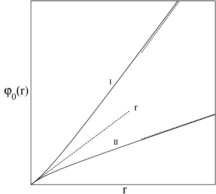
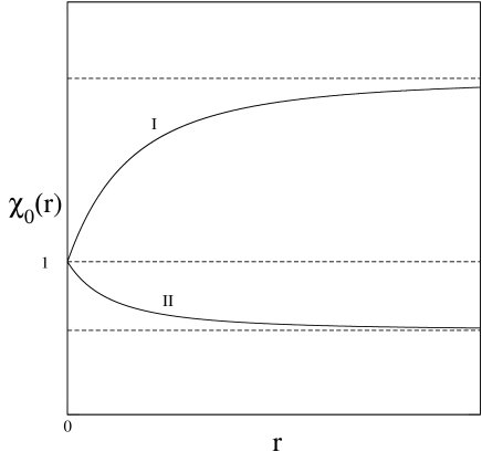
Figure 1: $I,V>0$ ; $II,V_{0}<0$, no bound states.

Figure 2: $I,V_{0}>0$ ; $II,V_{0}<0$, no bound states.

and iterate it, as we did with (29) for $\varphi_{0}$, to find the solution, which turns out now to be bounded everywhere. One then immediately sees on (36) that $\chi^{\prime}_{0}(0)$ is finite. We have, therefore, according to (13), and (33) or (34) (see Fig. 2) :

$$\left\{\begin{array}[]{l}\chi_{0}(0)=1\ ,\quad\chi_{0}(r)>0\ \hbox{for all $r$}\ ,\\ \\ \chi_{0}(r)\ \hbox{is a convex and decreasing function when $V_{0}>0$}\ ,\\ \\ \chi_{0}(r)\ \hbox{is a concave and increasing function when $V_{0}<0$,}\\ \hbox{with no bound states},\\ \\ \chi_{0}(\infty)=\displaystyle{{1\over A}}\not=0,\infty\ ;\ V_{0}>0\Rightarrow A>1\ ,\ V_{0}<0\Rightarrow A<1\ .\end{array}\right.$$ (37)

Consider now the mapping :

$$r\to x(r)={\varphi_{0}(r)\over\chi_{0}(r)}\ .$$ (38)

According to (37), this a perfectly regular and differentiable mapping, and is one to one since, according to (11), we have

$${dx\over dr}={\varphi^{\prime}_{0}\chi_{0}-\varphi_{0}\chi^{\prime}_{0}\over\chi_{0}^{2}(r)}={1\over\chi_{0}^{2}(r)}>0\ .$$ (39)

It follows then, since $\varphi_{0}(r\to\infty)\to\infty$, and $\chi_{0}(r\to\infty)\to{1\over A}\not=0,\infty$, that the mapping is one to one :

$$r\in[0,\infty)\Leftrightarrow x\in[0,\infty)\ ,\ x(0)=0\ ,\ x(\infty)=\infty\ .$$ (40)

In fact, this mapping is twice continuously differentiable since

$${d^{2}x\over dr^{2}}={-2\chi^{\prime}_{0}(r)\over\chi_{0}^{3}(r)}\ ,$$ (41)

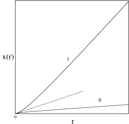
Figure 3: $I,V_{0}\geq 0$ ; $II,V_{0}<0$, no bound states.

and $\chi^{\prime}_{0}(r)$ is a continuous function of $r$ for $r\geq 0$. This last property follows from $\chi^{\prime\prime}_{0}(r)=V_{0}(r)\chi_{0}(r)$, where, by assumption, $V_{0}(r)\in L^{1}$ for $r>0$. Since $\chi_{0}(r)$ is a continuous function, $\chi^{\prime\prime}_{0}(r)$ is also $L^{1}$ for all $r>0$, and so $\chi^{\prime}_{0}(r)$ is continuous for $r>0$. $\chi^{\prime}_{0}$ cannot have jumps [9]. See Fig. 3.

Once we have established that the mapping (40) is regular and twice continuously differentiable, we can consider the equation

$$\left\{\begin{array}[]{l}\varphi^{\prime\prime}(r)=\left[V_{0}(r)+V_{1}(r)\right]\varphi(r)\ ,\\ \\ \varphi(0)=0\ ,\ \varphi^{\prime}(0)=1\ ,\end{array}\right.$$ (42)

where $V_{0}$ and $V_{1}$ satisfy the conditions shown in (8) and (9). We make now the change of variable and function

$$\left.r\to x={\varphi_{0}(r)\over\chi_{0}(r)}\ ,\quad\psi(x)={\varphi(r)\over\chi_{0}(r)}\right|_{r=r(x)}\ ,$$ (43)

where $r(x)$ is the inverse mapping, i.e. the inverse function of $x=x(r)$. Obviously, $r(x)$ is also twice continuously differentiable. Differentiating now twice $\psi$ with respect to $x$, and using (13), we easily find

$$\left.\ddot{\psi}(x)=\left[\chi_{0}^{4}(r)V_{1}(r)\right]\right|_{r=r(x)}\psi(x)\ .$$ (44)

There is no longer $V_{0}$ present. From the definition of $\psi(x)$, of $\varphi(r)$ given in (42), and (35), it is obvious that, because $\varphi(r)=r+o(1)$ as $r\to 0$, we have

$$\psi(0)=0\ ,\ \dot{\psi}(0)=\lim_{x\to 0}\dot{\psi}(x)=\lim_{r\to 0}\left[\varphi^{\prime}(r)\chi_{0}(r)-\varphi(r)\chi^{\prime}_{0}(r)\right]=1\ .$$ (45)

Suppose now that, from the beginning, $V_{1}(r)$ in (42) was of the form,

$${1\over\chi_{0}^{4}(r)}V_{1}\left(x={\varphi_{0}(r)\over\chi_{0}(r)}\right)\ ,$$ (46)

where $xV_{1}(x)\in L^{1}$ at $x=0$, and $x^{2}V_{1}(x)\in L^{1}$ at $x=\infty$. Then (44) would become

$$\left\{\begin{array}[]{l}\ddot{\psi}(x)=V_{1}(x)\ \psi(x)\ ,\\ \\ \psi(0)=0\ ,\ \dot{\psi}(0)=0\ ,\end{array}\right.$$ (47)

which we assume to be explicitely solvable. Then, from the definition (43), we would have for the solution of (42), with a $V_{1}$ of the form (46),

$$\varphi(r)=\chi_{0}(r)\ \psi\left({\varphi_{0}(r)\over\chi_{0}(r)}\right)\ .$$ (48)

Combining all these, with a slightly different notation, we have therefore the following

Theorem 1. The solution of

$$\left\{\begin{array}[]{l}\varphi^{\prime\prime}(r)=\left[V_{0}(r)+\displaystyle{{1\over\chi_{0}^{4}(r)}}V_{1}\left(\displaystyle{{\varphi_{0}(r)\over\chi_{0}(r)}}\right)\right]\varphi(r)\\ \\ \varphi(0)=0\ ,\ \varphi^{\prime}(0)=1\ ,\end{array}\right.$$ (49)

where $\varphi_{0}$ and $\chi_{0}$ are the two solutions of

$$\left\{\begin{array}[]{l}\varphi^{\prime\prime}_{0}(r)=V_{0}(r)\ \varphi_{0}(r)\ ,\\ \\ \varphi_{0}(0)=0\ ,\ \varphi^{\prime}_{0}(0)=1\ ,\ \hbox{no bound states,}\\ \\ \chi_{0}(r)\ \hbox{defined by (\ref{13e})},\chi_{0}(0)=1\ ,\end{array}\right.$$ (50)

is given by

$$\varphi(r)=\chi_{0}(r)\ \varphi_{1}\left({\varphi_{0}(r)\over\chi_{0}(r)}\right)\ ,$$ (51)

where $\varphi_{1}(x)$ is the (regular) solution of

$$\left\{\begin{array}[]{l}\ddot{\varphi}_{1}(x)=V_{1}(x)\ \varphi_{1}(x)\ ,\\ \\ \varphi_{1}(0)=0\ ,\ \dot{\varphi}_{1}(0)=1\ .\end{array}\right.$$ (52)

Therefore, if the Schrödinger equation at $k=0$ and $\ell=0$ can be explicitely solved for $V_{0}$ and $V_{1}$, then the solution of (49) is of the form (51). As we said in the introduction, one can check directly, that (51) is indeed the solution of (49). For bound states in (52) and (49), see below, after Remark 6.

Higher waves, $\ell{\bf>}$ 0. So far, we have been assuming $\ell=0$. It is easy to extend the results to the case $\ell>0$ in (50), i.e. to begin with

$$\varphi^{\prime\prime}_{0}(r)=\left[V_{0}(r)+{\ell(\ell+1)\over r^{2}}\right]\varphi_{0}(r)\ ,$$ (53)

and then add the potential $V_{1}$ in (49). $V_{0}$ is, as before, supposed to be such that $rV_{0}\in L^{1}$ at $r=0$, and $r^{2}V_{0}\in L^{1}$ at $r=\infty$. We shall see later that we need more rapid decrease at infinity. The regular solution $\varphi_{0}$ is usually normalized as follows

$$\varphi_{0}(r)={r^{2\ell+1}\over(2\ell+1)!!}+o\left(r^{\ell+1}\right)\ ,\quad r\to 0\ .$$ (54)

One can then combine (53) and (54) into the single Volterra integral equation

$$\varphi_{0}(r)={r^{\ell+1}\over(2\ell+1)!!}+\int_{0}^{r}{r^{2\ell+1}-r^{\prime 2\ell+1}\over(2\ell+1)r^{\ell}r^{\prime\ell}}V_{0}(r^{\prime})\varphi_{0}(r^{\prime})dr^{\prime}\ .$$ (55)

Solving this equation by iteration, one finds again, as for the case $\ell=0$, an absolutely and uniformly convergent series defining the solution $\varphi_{0}$, together with a bound similar to (30) for all finite $r\geq 0$ :

$$|\varphi_{0}(r)|\leq C\ r^{\ell+1}\exp\left(\int_{0}^{r}r^{\prime}|V_{0}(r)|dr^{\prime}\right)\leq C^{\prime}\ r^{\ell+1}\ ,$$ (56)

where $C$ and $C^{\prime}$ are absolute finite constants [1, 3, 4]. Using (56) in (55), one sees immediately that, for $r\to 0$,

$$\varphi_{0}(r)={r^{\ell+1}\over(2\ell+1)!!}+o\left(r^{2\ell+1}\right)\ ,\ \varphi^{\prime}_{0}(r)={r^{2\ell}\over(2\ell-1)!!}+o\left(r^{2\ell}\right)\ .$$ (57)

For all the above results, we need only $rV_{0}\in L^{1}(0)$. Also, by assumption, there are no bound states for (53). It follows again that, by the nodal theorem [7], $\varphi_{0}(r)$ cannot vanish for $r>0$. Because of (57), we find therefore that

$$\varphi_{0}(r)>0\ \hbox{for all $r>0$}\ .$$ (58)

From this, and (53), it follows immediately that if $V_{0}(r)>0$, then $\varphi_{0}(r)$ is convex. For $V_{0}(r)<0$, the situation is more subtle than for the case of $\ell=0$, nd $\varphi_{0}$ may become concave in some interval $(R_{1},R_{2})$.

We wish now to look at the behaviour of $\varphi_{0}(r)$ as $r\to\infty$. We assume here

$$r^{2\ell+2}\ V_{0}(r)\in L^{1}(\infty)\ .$$ (59)

Then we can let $r\to\infty$ in (55), to find

$$\varphi_{0}\ \mathrel{\mathop{\rm=}_{r\to\infty}}\ \left[{1\over(2\ell+1)!!}+\int_{0}^{\infty}{1\over 2\ell+1}r^{\prime-\ell}V_{0}(r^{\prime})\varphi_{0}(r^{\prime})dr^{\prime}\right]r^{\ell+1}$$ (60)

$$\qquad-{1\over 2\ell+1}\left[\int_{0}^{\infty}r^{\prime\ell+1}V_{0}(r^{\prime})\varphi_{0}(r^{\prime})dr^{\prime}\right]r^{-\ell}+\cdots$$

$$\qquad=A_{\ell}\ r^{\ell+1}+B_{\ell}\ r^{-\ell}+\cdots$$

Since $\varphi_{0}(r)$ never vanishes (absence of bound states), $A_{\ell}$ must be always positive. If $V_{0}>0$, then $A_{\ell}>1$, and if $V_{0}<0$, $0<A_{\ell}<1$. For $B_{\ell}$, it is just the opposite. These are quite the same as for $\ell=0$.

We can now define the second (independent) solution $\chi_{0}(r)$ by (13) again, and we find now, using (57) and (60), that

$$\left\{\begin{array}[]{l}\chi_{0}(r)=\displaystyle{{(2\ell-1)!!\over r^{\ell}}}+\cdots\ ,\quad r\to 0\\ \\ \chi_{0}(r)=\displaystyle{{1\over(2\ell+1)A_{\ell}}}r^{-\ell}\ ,\quad r\to\infty\ .\end{array}\right.$$ (61)

If we introduce the same variable $x=x(r)$ as before

$$x=x(r)={\varphi_{0}(r)\over\chi_{0}(r)}\ ,$$ (62)

we find

$$\left\{\begin{array}[]{l}x(r)=A\ r^{2\ell+1}+\cdots\ ,\quad r\to 0\\ \\ x(r)=B\ r^{2\ell+1}\ ,\quad r\to\infty\ .\end{array}\right.$$ (63)

The rest of the analysis goes as before, and we find

Theorem 2. Theorem 1 is valid if we add $\ell(\ell+1)/r^{2}$ to $V_{0}$ in (49) and (50), i.e.

$$\left\{\begin{array}[]{l}\varphi^{\prime\prime}(r)=\left[\left(V_{0}(r)+\displaystyle{{\ell(\ell+1)\over r^{2}}}\right)+\displaystyle{{1\over\chi_{0}^{4}(r)}}V_{1}\left(\displaystyle{{\varphi_{0}(r)\over\chi_{0}(r)}}\right)\right]\varphi(r)\ ,\\ \\ \varphi(r\to 0)=\displaystyle{{r^{\ell+1}\over(2\ell+1)!!}}+\cdots\end{array}\right.$$ (64)

and

$$\left\{\begin{array}[]{l}\varphi^{\prime\prime}_{0}(r)=\left[V_{0}(r)+\displaystyle{{\ell(\ell+1)\over r^{2}}}\right]\varphi_{0}(r)\ ,\ r^{2\ell+2}\ V_{0}(r)\in L^{1}(\infty)\ ,\\ \\ \varphi_{0}(r\to 0)=\displaystyle{{r^{\ell+1}\over(2\ell+1)!!}}+\cdots\ ,\ \hbox{no bound states,}\end{array}\right.$$ (65)

$\chi_{0}(r)$ defined by (13), $\chi_{0}(r\to 0)={(2\ell-1)!!\over r^{\ell}}$, while (52) remains unchanged. The solution is again provided by (51). This can also be checked directly.

Remark 5. Since the behaviour of $\varphi_{1}(x)$ is $x+\cdots$ as $x\to 0$, and $\varphi_{0}(r)/\chi_{0}(r)=r^{2\ell+1}$ as $r\to 0$, it is obvious on (51) that we have, as we should,

$$\varphi(r)=\alpha_{\ell}\ r^{\ell+1}+\cdots\ ,\quad r\to 0\ .$$ (66)

Likewise, it is easy to find

$$\varphi(r)=\beta_{\ell}\ r^{\ell+1}+\gamma_{\ell}\ r^{-\ell}\ ,\quad r\to\infty\ .$$ (67)

Bound States. So far, we have assumed that there are no bound states in (52). If there are $n$ bound states with $V_{1}(x)$, i.e. in (52), which is the same for Theorem 1 and Theorem 2, this means that $\varphi_{1}$ has $n$ nodes for $x>0$. And we have also $n$ nodes for the full solution $\varphi$, given always by (51). The potentials $V_{1}$ and $V$ have the same number of bound states. But, of course, the binding energies are different.

Remark 6. As we said in Remark 3, once we have $V(r)$ and $\varphi(r)$, we can now start again with $V_{0}$ and $V$ instead of $V_{0}$ and $V_{1}$, and proceed as before. This process can be repeated as many times as we wish, and we get more and more potentials for which the radial Schrödinger equation at zero energy can be solved. Also, the number of bound states, if any, remains the same. Unfortunately, the potentials and the wave functions become quickly very complicated. However, one may ask what will happen at the limit of infinite repetitions. This question is certainly not easy to answer.

Singular Potentials. As we said in the introduction, the radial equation can be solved at $k=0$ and for all $\ell$ for singular potentials which are just inverse powers potentials shown in (18). The solutions are given in terms of modified Bessel and Hankel functions. We shall see explicit examples in the next section. One more class is given by [6, 10]

$$V_{0}(r)={g_{1}\over r^{2}\left({\rm Log}\ {1\over r}\right)^{p}}+{g_{2}\over r^{2}\left({\rm Log}\ {1\over r}\right)^{2}}+{\ell(\ell+1)\over r^{2}}\ ,$$ (68)

with $p<2$, $g_{1}>0$. These potentials must be cut at $r=R_{0}<1$ in order to avoid none integrable singularities at $r=1$. The solution is given in terms of Whittaker functions [6, 10]. Once we know the solution $\varphi_{0}(r)$, we can proceed as before, and add a regular potential $V_{1}$ with any (finite) number of bound states.

We should mention here that, contrary to the case of regular potentials at the origin, i.e. those for which $rV_{0}(r)\in L^{1}$ at $r=0$, here, because of strong singularities at $r=0$, we find [1, 6] $\varphi_{0}(0)=\varphi^{\prime}_{0}(0)=\cdots\varphi_{0}^{(n)}(0)=\cdots=0$. All the derivatives of $\varphi_{0}$ vanish at $r=0$. The normalization is therefore arbitrary, and cannot be made at $r=0$. Once this is chosen (usually by the behaviour of $\varphi$ at $r=\infty$), then $\chi_{0}(r)$ is given again by (13), and we have the Wronskian $W(\varphi_{0},\chi_{0})=1$. Usually, in such a case, it is customary to normalize $\varphi_{0}$ at infinity, according to

$$\varphi_{0}(r)=r+C+o(1)\ ,\ r\to\infty\ ,$$

which entails also

$$\chi_{0}(r)=r+C^{\prime}+o(1)\ ,\ r\to\infty\ .$$

As we shall see on explicit examples in the next section, our procedure for generating new potentials can go on without modifications.

III. Examples

1. Regular Potentials. We have already given, in the introduction, as examples for the applications of Theorems 1 and 2, the solutions of the Schrödinger equation for $\ell=0$, $V_{0}=(7)$, $V_{1}=(6)$, or $V_{0}=(6)$ together with $\ell(\ell+1)/r^{2}$, and $V_{1}=(7)$. They are given by formulae (22)-(26). More examples are obtained by combining any two potentials among those given by (2) to (7). We need only the solutions $\varphi$ and $\chi$, the latter defined by (13), for these potentials.

a. Exponential potential

$$\left\{\begin{array}[]{l}V(r)=\lambda e^{-\mu r}\ ,\ \lambda>0\ ,\ \mu>0\ ,\ \ell=0\\ \\ \varphi(r)=\alpha\ I_{0}\left(\displaystyle{{2\sqrt{\lambda}\over\mu}}e^{-\mu r/2}\right)+\beta\ K_{0}\left(\displaystyle{{2\sqrt{\lambda}\over\mu}}e^{-\mu r/2}\right)\ ,\\ \\ \chi(r)=\displaystyle{{I_{0}\left({2\sqrt{\lambda}\over\mu}e^{-\mu r/2}\right)\over I_{0}\left({2\sqrt{\lambda}\over\mu}\right)}}\ ,\quad\chi(0)=1\ ,\quad\chi(\infty)=\displaystyle{{1\over I_{0}\left({2\sqrt{\lambda}\over\mu}\right)}}\ .\end{array}\right.$$

$I_{0}$ and $K_{0}$ are modified Bessel and Hankel functions of order zero, and the constants $\alpha$ and $\beta$ are determined to have $\varphi(0)=0$ and $\varphi^{\prime}(0)=1$. It is then easy to show that, according to our general analysis of section II, we have

$$\varphi(r\to\infty)=I_{0}\left({2\sqrt{\lambda}\over\mu}\right)r+\cdots$$

The presence of $r$ in (71) is due to the presence of $\log z$ in $K_{0}(z)$ where $z\to 0$ [8].

b. The potential (5) for $\alpha>0$, $\ell\geq 0$. The solutions $\varphi$ and $\chi$ are given by combinations of hypergeometric functions of appropriate arguments. We refer the reader to [5] for details.

c. Hulthén Potential ($3$), $\ell=0$. Here also, the solutions $\varphi$ and $\chi$ are given in terms of appropriate hypergeometric functions $F$. See [1, 4] for details.

2. Singular Potentials [6]. Here, we consider only three cases.

d. Inverse Power Potentials, $\ell\geq 0$ :

$$\left\{\begin{array}[]{l}V(r)=\displaystyle{{g\over r^{n}}}\ ,\quad g>0\ ,\quad n>2\ell+3\ ,\\ \\ \varphi(r)=r^{1/2}K_{{2\ell+1\over n-2}}\left(\displaystyle{{2\sqrt{g}\over(n-2)r^{{n-2\over 2}}}}\right)\ ,\\ \chi(r)=r^{1/2}\left[\alpha K_{{2\ell+1\over n-2}}\left(\displaystyle{{2\sqrt{g}\over(n-2)r^{{n-2\over 2}}}}\right)+\beta I_{{2\ell+1\over n-2}}\left(\displaystyle{{2\sqrt{g}\over(n-2)r^{{n-2\over 2}}}}\right)\right.\ ,\end{array}\right.$$

where $I_{\nu}$ and $K_{\nu}$ are modified Bessel and Hankel functions. We must choose $n>2\ell+3$ in order to comply with (60) [6].

The parameters $\alpha$ and $\beta$ are determined for having $\chi(r)$ to comply with the asymptotic behaviours deduced from (13), for $r\to 0$ and $r\to\infty$. One has to remember the Wronkian

$$W\left[r^{1/2}\ K_{\nu}\left(\beta r^{\sigma}\right),r^{1/2}I_{\nu}\left(\beta r^{\sigma}\right)\right]=\sigma\ .$$

The case $\ell=0$, $n=4$ is particulary simple. One finds

$$\left\{\begin{array}[]{l}V(r)=\displaystyle{{g\over r^{4}}}\ ,\quad g>0\ ,\quad\ell=0\ ,\\ \\ \varphi(r)=re^{-\sqrt{g}/r}\ \displaystyle{\mathrel{\mathop{\rm=}_{r\to\infty}}}\ r-\sqrt{g}+\cdots\\ \\ \chi(r)=\displaystyle{{r\over\sqrt{g}}}\sinh\left(\displaystyle{{\sqrt{g}\over r}}\right)\ \displaystyle{\mathrel{\mathop{\rm=}_{r\to\infty}}}\ 1+\cdots\end{array}\right.$$

e. Logarithmic Potentials [6, 10]. We consider here the simplest case of (68) with $p=1$, and any angular momentum $\ell\geq 0$ :

$$\left\{\begin{array}[]{l}V(r)=\left[\displaystyle{{\alpha\over r^{2}\ {\rm Log}\left({1\over r}\right)}}+\displaystyle{{g\over r^{2}\ {\rm Log}^{2}\ \left({1\over r}\right)}}\right]\theta(R-r)\ ,\ \alpha>0\ ,\ R<1\ ,\\ \\ \varphi(r)=r^{1/2}\left[\displaystyle{{\Gamma(-2\nu)\over\Gamma\left({1\over 2}-\nu-\mu\right)}}\ M_{\mu,\nu}(x)\right.\\ \qquad\left.+\displaystyle{{\Gamma(2\nu)\over\Gamma\left({1\over 2}+\nu-\mu\right)}}\ M_{\mu,-\nu}(x)\right]\ ,\\ \\ \chi(r)=r^{1/2}\left[\alpha\ M_{\mu,\nu}(x)+\beta M_{\mu,-\nu}(x)\right]\ ,\end{array}\right.$$

where $M_{\mu,\nu}$ are Whittaker functions [8],

$$x=(2\ell+1){\rm Log}\ {1\over r}\ ,\quad k={-\alpha\over 2\ell+1}\ ,\quad\nu=i\sqrt{g-{1\over 4}}\ ,$$

and $\alpha$ and $\beta$ are determined according to (13) for $r\to 0$ and $r\to\infty$. Note here that, for $r\geq R$, we have the free equation (no potential), and, therefore, we must first adjust the free solution to the interior solution at $r=R$, as usual.

Note here that the singular part of the potential is just the first potential, and that is why we must choose $\alpha>0$. The second potential is regular since it satisfies $rV(r)\in L^{1}(0)$. We can therefore choose $g\ {{\textstyle>}\atop{\textstyle<}}\ 0$. There are several more examples of singular potentials for which the radial equation can be solved explicitely. We refer the reader for details to [6].

f. Coulomb Potential. The Coulomb potential is regular at the origin, and so we have the usual solutions $\varphi$ and $\chi$, as defined previously. We choose, of course, the repulsive case. The solutions can be read off from (72) adapted to $n<2$, or else, be obtained in the standard way [1, 4]. One has, for $\ell=0$ :

$$\left\{\begin{array}[]{l}V=\displaystyle{{\alpha\over r}}\ ,\quad\alpha>0\ ,\quad\ell=0\ ,\\ \\ \varphi(r)=\displaystyle{\sqrt{{r\over\alpha}}}\ I_{1}(2\sqrt{\alpha r})\ ,\\ \\ \chi(r)=-\pi\sqrt{\alpha r}\ K_{1}\left(2\sqrt{\alpha r}\right)\ ,\end{array}\right.$$

where $I_{1}$ and $K_{1}$ are the modified Bessel and Hankel functions, and similar formulae for $\ell>0$. As we see here, the long range tail of the potential leads to the exponential growth of $\varphi$ at $r\to\infty$, $\varphi\sim r^{1/4}\exp(2\sqrt{\alpha r})$, and the exponential decrease of $\chi(r)\sim r^{1/4}\exp(-2\sqrt{\alpha r})$, to zero. This does not affect the validity of the change of variable $r\to x=\varphi/\chi$, etc, of section II, except that now $x$ grows exponentially as $r\to\infty$. Note that $I_{1}$ and $K_{1}$ do not vanish, $I_{1}$ for $r>0$, and $K_{1}$ for $r<\infty$ [8]. $\varphi$ is again an increasing convex function, and $\chi$ a decreasing convex function. The only difference with the short-range potentials is that, now, $\chi^{-4}(r)$ grows exponentially, so that, in (49) and (64), if $V_{0}$ is chosen to be the Coulomb potential, the second potential may seem to become infinite as $r\to\infty$ ($x\to\infty$). However, we have always assumed $V_{1}(r)$ to be short range, i.e. decreasing fast enough at infinity. It follows that $\chi_{0}^{-4}(r)V_{1}(x)$ is again short range. For instance, if $V_{1}(r)\sim r^{-4}$, then $\chi_{0}^{-4}V_{1}(r)\sim 1/(x^{2}{\rm Log}^{2}x)$, etc, i.e. $x\chi_{0}^{-4}V_{1}$ is $L^{1}$ in $x$ at $x=\infty$.

Other long range potentials of the form $g/r^{n}$, $n<2$, can be dealt with in the same way by adapting (72) to $n<2$, and one reaches similar conclusions as for the Coulomb potential. As for confining potentials like the harmonic oscillator, etc, we shall consider them in a separate paper.

Concluding remarks.

So far, all the potentials for which the radial Schrödinger equation has been shown to be soluble analytically in closed form have their solutions given by various hypergeometric functions in appropriate variables [1, 3, 4, 6]. In fact, in many instances, as we have seen on examples, the hypergeometric functions simplify to Bessel and Hankel functions of real or imaginary arguments. The only exceptions are Bargmann potentials [1, 3], for which the solutions are given in terms of rational functions of $\sinh\alpha_{j}r$, $\cosh\alpha_{j}r$, $\sin\beta_{j}r$, and $\cos\beta_{j}r$, $j=1,\cdots n$, where $\alpha_{j}$ and $\beta_{j}$ are given by the positions of the poles and zeros of the $S$-matrix, and the $r^{-4}$ potential [2], for which the solution is given in terms of Mathieu functions.

In the present paper, as seen on (49) and (64), the potentials themselves have their arguments given by ratios of hypergeometric functions, and the solutions are then hypergeometric functions of ratios of hypergeometric functions, as seen on (51). And this process can be repeated indefinitely, as we saw before. One may then ask what the potentials and their wave functions become in the limit. Also, we saw that, for both $V_{0}$ and $V_{1}$, we can take potentials which are very singular but repulsive at the origin, like $gr^{-n}$ and $\lambda r^{-m}$, $g>0$, $\lambda>0$, $m,n>2$. All kinds of combinations are therefore possible for $V_{0}$ and $V_{1}$.

It is trivial to construct infinitely many potentials for which the Schrödinger equation could be solved at zero energy. One can choose any positive, convex, and twice continously differentiable function, which is decreasing, and such that

$$\chi_{0}(0)=1\ ,\quad\chi_{0}(\infty)={1\over A}\ ,\quad 1<A<\infty\ ,$$

and write

$$V_{0}(r)={\chi^{\prime\prime}_{0}(r)\over\chi_{0}(r)}\ .$$

If $\chi_{0}(r)$ is decreasing fast enough to $A^{-1}$ at infinity, then $V_{0}(r)$ is short-range. $\varphi_{0}(r)$ is defined here by $(13^{\prime})$. Example :

$$\left\{\begin{array}[]{l}\chi_{0}(r)=\displaystyle{{1\over(1+\alpha)}}\left[1+\displaystyle{{\alpha\over(1+\beta r)^{n}}}\right]\ ,\\ \\ \alpha>0\ ,\ \beta>0\ ,\ n>1\ .\end{array}\right.$$

According to (78), we have

$$V_{0}(r)={\alpha n(n+1)\over(1+\alpha)(1+\beta r)^{n+2}\chi_{0}(r)}\ \mathrel{\mathop{\sim}_{r\to\infty}}\ r^{-n-2}\ .$$

However, all this is valid for this particular $V_{0}(r)$. If we try to introduce a coupling constant $\lambda$ in front of $V_{0}(r)$, i.e. try to solve

$$\chi^{\prime\prime}(r)=\lambda V_{0}(r)\ \chi(r)\ ,$$

we usually do not find explicit solutions. This is indeed the case here.

Next, consider

$$\chi_{0}(r)={1+e^{-\mu r}\over 2}\ ,\ \mu>0\ ,$$

where $A=2$. This leads to

$$V_{0}(r)={\chi^{\prime\prime}_{0}(r)\over\chi_{0}(r)}={\mu^{2}e^{-\mu r}\over 1+e^{-\mu r}}\ .$$

$\varphi_{0}(r)$ is then easily calculated from ($13^{\prime}$). In this case, one can solve (81) for any $\lambda$ since (83) is a particular case of (4), and the solutions are given, in general, in terms of hypergeometric functions [4]. Only for $\lambda=1$, they reduce to the simple form (82) for $\chi_{0}$, and the corresponding $\varphi_{0}(r)$.

Acknowledgments. One of the authors (KC) would like to thank the Department of Mathematics of the Science University of Tokyo, and Professors Kenro Furutani, Reido Kobayashi, and Takao Kobayashi, for warm hospitality and generous financial support when this work began.

References

[1] Newton R G 1982 Scattering Theory of Waves and
Particles (New York : Springer). See especially Chapter 14 for
examples, i.e. potentials for which the Schrödinger equation can be
solved.
[2] Spector R M 1964 J. M. Phys. 5 1185.
[3] Chadan K and Sabatier PC 1989 Inverse Problems in Quantum
Scattering Theory 2nd edn (Berlin : Springer).
[4] Galindo A and Pascual P 1990 Quantum Mechanics two
volumes (Berlin : Springer).
[5] Cheng H 1966 Nuovo Cim 45 487.
[6] Frank W M, Land D J, and Spector M 1971 Rev. Modern
Physics 43 36.
[7] Courant R and Hilbert D 1953 Methods of Mathematical
Physics vol. I (New York : Interscience).
[8] Magnus M and Oberhettinger F 1949 Formulas and Theorems
for the Functions of Mathematical Physics (New York : Chelsea
Publishing Company) ; Erdélyi A (ed) 1953 Higher Transcendental Functions vol. II (New York : Mc Graw Hill)
[9] Hille E 1969 Lectures on Ordinary Differential
Equations (Reading, MA : Addison-Wesley) ; Royden H L 1968 Real
Analysis 2nd edn (New York : McMillan) ; Titchmarsh E C 1960 The
Theory of Functions 2nd edn (Oxford : Oxford University Press).
[10] Chadan K and Musette M 1993 C. R. Ac. Sci. Paris 316II 1.