Supersymmetric Extensions of Calogero–Moser–Sutherland like Models: Construction and Some Solutions

Abstract

We introduce a new class of models for interacting particles. Our construction is based on Jacobians for the radial coordinates on certain superspaces. The resulting models contain two parameters determining the strengths of the interactions. This extends and generalizes the models of the Calogero–Moser–Sutherland type for interacting particles in ordinary spaces. The latter ones are included in our models as special cases. Using results which we obtained previously for spherical functions in superspaces, we obtain various properties and some explicit forms for the solutions. We present physical interpretations. Our models involve two kinds of interacting particles. One of the models can be viewed as describing interacting electrons in a lower and upper band of a one–dimensional semiconductor. Another model is quasi–two–dimensional. Two kinds of particles are confined to two different spatial directions, the interaction contains dipole–dipole or tensor forces.

I Introduction

There is an intimate relation between group theory and certain one–dimensional exactly solvable systems HC ; HC1 ; gel50 ; ber57 ; HEL . The radial part of the Laplace–Beltrami operator on symmetric spaces induces in a natural way an interacting one–dimensional many–body Hamiltonian with a characteristic $gv^{-2}(x_{n}-x_{m})$ interaction between the particles at positions $x_{n}$ and $x_{m}$. Here, $g$ is the coupling constant and the function $v$ may be a sine, a hyperbolic sine or the identity, depending on the curvature of the symmetric space under consideration. These and similar systems have been studied first by Calogero and Sutherland cal69 ; cal71 ; sut72 . They have much in common with the Brownian motion model studied by Dyson as early as in 1962 DYS1 ; DYS2 . Other forms of the potential have been introduced, such as the Toda lattice gut80a ; gut80b or the Weierstrass function, which generalizes the original form of interaction. We refer to all models as Calogero–Moser–Sutherland (CMS) models irrespectively of the interaction potential and the underlying Lie algebra.

The first proof of exact integrability of some CMS–Hamiltonians have been given in OP77 . Later a more general proof has been given in heck87 ; heck91 by very different arguments. In this context, we also refer to the work in Ref. etin95 .

More recently, these models have been studied in the framework of supersymmetric quantum mechanics susy1 ; susy2 . Although we work with supersymmetry as well, our approach is different from this. Generalizations to higher space dimensions gos97 ; kah98 ; MEL04b have also been proposed. Extensive reviews are given in Refs. OP ; CAL .

Our supersymmetric construction extends and generalizes the group theoretical approach in ordinary spaces by exploring the relation between the radial part of Laplace operators on symmetric superspaces and certain Schrödinger operators: In some cases, i.e. for special values of the coupling constant $g$, the solution of the interacting particle Hamiltonian can be written as an integral over the classical matrix groups, the orthogonal, the unitary and the symplectic group. These groups are labeled by the Dyson index $\beta=1,2,4$, respectively. The coupling constant $g$ is a function of the Dyson index $\beta$. Similar relations for Schrödinger operators exist also in superspace TG ; GUH4 ; GUKOP2 ; GUKO2 . A classification of matrix supergroups and more general of symmetric superspaces has been given in Ref. MRZ1 . In this contribution, we introduce a labeling of symmetric superspaces in terms of a pair of numbers $(\beta_{1},\beta_{2})$ akin to Dyson’s index $\beta$ in ordinary space. This label may further be continued analytically in $\beta_{1}$ and $\beta_{2}$ to arbitrary combinations $(\beta_{1},\beta_{2})$. Our construction leads to a natural supersymmetric generalization of the CMS model for interacting particles. Hence, we arrive at a new class of many-body systems. They are likely to be exactly solvable in the allowed parameter region.

Our construction goes considerably beyond the one by Sergeev and Veselov ser ; serves1 ; serves2 . These authors arrived at superanalogues of CMS models, starting from the underlying root spaces of the superalgebra. They also give a solution in terms of superanalogues of Jack polynomials. Their models however, depend only on one parameter and are therefore different from ours which crucially depend on two. Some of our models are related to the many species generalization of CMS models in Refs. MEL03 ; MEL04a . In contrast to our approach, the latter construction is ad hoc and it is not based on superspaces.

The models we are investigating have been communicated in guk05 , where emphasis was put on their interpretation and possible applications. Here we focus on mathematical aspects of the models. In particular the question of exact solvablity is discussed and exact solutions for certain parameters $\beta_{1}$, $\beta_{2}$ are presented.

The paper is organized as follows: For the convenience of the reader we briefly compile some results for the models for interacting particles in ordinary space in Section II. Various supersymmetric generalizations of the models for interacting particles are presented in Section III. In Section IV, we find certain solutions by deriving a new recursion formula. In Section V, we give an extensive interpretation of the physical systems described by the supersymmetric models. A brief version of this section can be found in guk05 . We summarize and conclude in Section VI.

II Models for Interacting Particles in Ordinary Space

In Section II.1, we sketch the connection between ordinary groups and the many–particle Hamiltonian. We discuss the connection to the recursion formula in Section II.2.

II.1 Differential Equation and its Interpretation

The connection between some models of the CMS type in ordinary space and some radial Laplaceans appearing in group theory OP is seen by considering the eigenvalue equation

$$\Delta_{x}^{(\beta)}\Phi_{N}^{(\beta)}(x,k)=-\left(\sum_{n=1}^{N}k_{n}^{2}\right)\Phi_{N}^{(\beta)}(x,k)\ .$$ (1)

The $N$ variables $x_{n},\ n=1,\ldots,N$ are interpreted as the positions of the particles later on. There is a further set of $N$ variables $k_{n},\ n=1,\ldots,N$ which will play the rôle of quantum numbers. The operator $\Delta_{x}$ depends on a parameter $\beta$ and is given by

$$\Delta_{x}^{(\beta)}=\sum_{n=1}^{N}\frac{1}{|\Delta_{N}(x)|^{\beta}}\frac{\partial}{\partial x_{n}}|\Delta_{N}(x)|^{\beta}\frac{\partial}{\partial x_{n}}\ ,$$ (2)

where

$$\Delta_{N}(x)=\prod_{n<m}(x_{n}-x_{m})$$ (3)

is the Vandermonde determinant. If the symmetry condition $\Phi_{N}^{(\beta)}(x,k)=\Phi_{N}^{(\beta)}(k,x)$ and the initial condition $\Phi_{N}^{(\beta)}(0,k)=1$ are required, the solution of the eigenvalue equation (1) is for $\beta=1,2,4$ equivalent to group integrals over ${\rm O}(N)$, ${\rm U}(N)$ and ${\rm USp}(2N)$, respectively. These integrals are referred to as spherical functions HEL1 . We notice that they are different from the group integral which Harish–Chandra investigated in Ref. HC ; HC1 . This is reflected in the operator (2), which is the radial Laplacean on symmetric spaces with zero curvaturegin62 , more precisely on the spaces of symmetric, Hermitean, and Hermitean selfdual matrices for $\beta=1,2,4$. Only for $\beta=2$, the Laplacean coincides with the Laplacean over the algebra of the group ${\rm U}(N)$. This is the only case where the spherical function is identical to a Harish–Chandra group integral due to the vector space isomorphism of Hermitean and anti Hermitean matrices. For arbitrary $\beta$ the eigenvalue equation (1) is closely connected to models of one dimensional interacting particles. Using the ansatz

$$\Phi_{N}^{(\beta)}(x,k)=\frac{\Psi_{N}^{(\beta)}(x,k)}{\Delta_{N}^{\beta/2}(x)\Delta_{N}^{\beta/2}(k)}$$ (4)

the eigenvalue equation (1) is reduced to a Schrödinger equation

$$\left(\sum_{n=1}^{N}\frac{\partial^{2}}{\partial x_{n}^{2}}-\beta\left(\frac{\beta}{2}-1\right)\sum_{n<m}\frac{1}{(x_{n}-x_{m})^{2}}\right)\Psi_{N}^{(\beta)}(x,k)\ =-\left(\sum_{n=1}^{N}k_{n}^{2}\right)\Psi_{N}^{(\beta)}(x,k)\ ,$$ (5)

which contains a kinetic part and a distance dependent interaction. Often, one adds $N$ confining potentials to the interaction in Eq. (5). This is done to make the system a bound state problem. However, apart from this, the structure of the model is not significantly affected by this modification. Thus, we will not work with confining potentials in the sequel. The specific model Eq. (5) is also called rational CMS model serves1 or free CMS model.

The solution $\Psi_{N}^{(\beta)}(x,k)$ is now interpreted as a wave function of the Schrödinger equation (5) with energy $\sum k_{n}^{2}$. Thus, no symmetry condition such as $\Psi_{N}^{(\beta)}(x,k)=\Psi_{N}^{(\beta)}(k,x)$ is imposed. In the following we always refer to functions such as $\Psi_{N}^{(\beta)}(x,k)$ as wave function. On the other hand, functions such as $\Phi_{N}^{(\beta)}(k,x)$ and more general solutions of eigenvalue equations of type (1) are referred to as matrix Bessel functions.

The parameter $\beta>0$ measures the strength of the inverse quadratic interaction. The interaction can be attractive $\beta<2$ or repulsive $\beta>2$. For $\beta=2$, the model is interaction free. This is group theoretically the unitary case and equivalent to the Itzykson–Zuber derivation IZ of the ${\rm U}(N)$ Harish–Chandra integral.

The symmetric spaces mentioned above stem from a common larger group, namely the special linear group. In Cartan s classification they are referred to as ${\rm A}$, ${\rm AI}$ and ${\rm AII}$ HEL . There are other symmetric spaces derived from the orthogonal and the symplectic groups as larger groups, designated ${\rm B}$, ${\rm C}$ and ${\rm D}$, respectively. These symmetric spaces are also related to Schrödinger equations, but with a different interaction OP .

II.2 Connection to the Recursion Formula for Radial Functions

For arbitrary positive $\beta$ the solutions of the eigenvalue equation (1) $\Phi_{N}^{(\beta)}(x,k)$ can be expressed in terms of a recursion formula GUKOP1 ; GUKO1

$$\Phi_{N}^{(\beta)}(x,k)\ =\ \int d\mu(x^{\prime},x)\,\exp\left(i\left(\sum_{n=1}^{N}x_{n}-\sum_{n=1}^{N-1}x_{n}^{\prime}\right)k_{N}\right)\,\Phi_{N-1}^{(\beta)}(x^{\prime},\widetilde{k})\ ,$$ (6)

where $\Phi_{N-1}^{(\beta)}(x^{\prime},\widetilde{k})$ is the solution of the Laplace equation (1) for $N-1$. Here, $\widetilde{k}$ denotes the set of quantum numbers $k_{n},\ n=1,\ldots,(N-1)$ and $x^{\prime}$ the set of integration variables $x_{n}^{\prime},\ n=1,\ldots,(N-1)$. The integration measure is

$$d\mu(x^{\prime},x)\ =\ G_{N}^{(\beta)}\,\frac{\Delta_{N-1}(x^{\prime})}{\Delta_{N}^{\beta-1}(x)}\,\left(-\prod_{n,m}(x_{n}-x_{m}^{\prime})\right)^{\beta/2-1}\,d[x^{\prime}]\ .$$ (7)

Here, $d[x^{\prime}]$ is the product of all differentials $dx_{n}^{\prime},\ n=1,\ldots,(N-1)$. The constant $G_{N}^{(\beta)}$ guarantees a proper normalization. The inequalities

$$x_{n}\ \leq\ x_{n}^{\prime}\ \leq\ x_{n+1}\ ,\qquad n=1,\ldots,(N-1)$$ (8)

define the domain of integration. An equivalent recursion formula exists also for the eigenfunctions $\Psi_{N}^{(\beta)}(x,k)$ of the Hamiltonian in Eq. (5). For $\beta=1,2,4$ the above recursion formula is equivalent to group integrals over ${\rm O}(N)$, ${\rm U}(N)$ and ${\rm USp}(2N)$, respectively. The case of arbitrary $\beta$ has not found a clear group theoretical or geometrical interpretation yet. However, many properties which are obvious for the group integral carry over to arbitrary $\beta$. We just mention the following. $\Phi_{N}^{(\beta)}(x,k)$ is a symmetric function in both sets of arguments. This has as a direct consequence that the behavior under particle exchange of the wave function $\Psi_{N}^{(\beta)}(x,k)$ is only governed by the Vandermonde determinant $\Delta_{N}^{\beta/2}(x)\Delta_{N}^{\beta/2}(k)$. The wave function obtains under particle exchange a complex phase

$$P_{nm}\Psi_{N}^{(\beta)}(x,k)=\exp(-i\pi\beta/2)\Psi_{N}^{(\beta)}(x,k)\ ,$$ (9)

with

$$P_{nm}\Psi_{N}^{(\beta)}(x_{1},\ldots,x_{n},\ldots,x_{m},\ldots,k)=\Psi_{N}^{(\beta)}(x_{1},\ldots,x_{m},\ldots,x_{n},\ldots,k)\ .$$ (10)

For this reason the model of Eq. (5) is frequently used as paradigm for systems with anionic statistics Ha ; Wi . A recursion formula akin to Eq. (6) has also been derived for Jack polynomials OO .

III Models for Interacting Particles in Superspace

A classification of supergroups and superalgebras similar to Cartan’s classification in ordinary space can be found in Refs. KAC1 ; KAC2 . Apart from some exotic groups, there are essentially only two families of supergroups. The general linear supergroup ${\rm GL}(k_{1}/k_{2})$ respectively its compact version the unitary supergroup ${\rm U}(k_{1}/k_{2})$ and the orthosymplectic group ${\rm OSp}(k_{1}/2k_{2})$. A classification of the symmetric superspaces has been given in Ref. MRZ1 .

In Sections III.1 and III.2 we present supersymmetric generalizations of models for interacting particles based on the supergroups ${\rm GL}(k_{1}/k_{2})$ and on the symmetric superspaces ${\rm GL}(k_{1}/2k_{2})/{\rm OSp}(k_{1}/2k_{2})$. In Section III.4, we give the supersymmetric generalization based on the supergroup ${\rm OSp}(k_{1}/2k_{2})$. In Sections III.3 and  III.5 we introduce two more general models which comprise the other models derived before as special cases. These models can be considered as supersymmetric generalization of the Schrödinger equation (5) for the CMS models in ordinary space.

III.1 Models Derived from the Superspace ${\rm GL}(k_{1}/k_{2})$

To extend the models in ordinary space to superspace, we begin with models derived from the superunitary case. The underlying symmetric superspace is called ${\rm A|A}$ in Ref. MRZ1 . We construct the eigenvalue equation

$$\Delta_{s}^{({\rm u},\beta)}\lambda_{k_{1}k_{2}}^{(\beta)}(s,r)=-\frac{1}{\sqrt{\beta}}\left(\sum_{p=1}^{k_{1}}r_{p1}^{2}+\sum_{p=1}^{k_{2}}r_{p2}^{2}\right)\lambda_{k_{1}k_{2}}^{(\beta)}(s,r)\ .$$ (11)

for the operator

$$\Delta_{s}^{({\rm u},\beta)} = \frac{1}{\sqrt{\beta}}\sum_{p=1}^{k_{1}}\frac{1}{B_{k_{1}k_{2}}^{\beta}(s)}\frac{\partial}{\partial s_{p1}}B_{k_{1}k_{2}}^{\beta}(s)\frac{\partial}{\partial s_{p1}}+\frac{1}{\sqrt{\beta}}\sum_{p=1}^{k_{2}}\frac{1}{B_{k_{1}k_{2}}^{\beta}(s)}\frac{\partial}{\partial s_{p2}}B_{k_{1}k_{2}}^{\beta}(s)\frac{\partial}{\partial s_{p2}}\ ,$$ (12)

where the function TG ; GGT

$$B_{k_{1}k_{2}}(s)=\frac{\prod_{p<q}(s_{p1}-s_{q1})\prod_{p<q}(s_{p2}-s_{q2})}{\prod_{p,q}(s_{p1}-is_{q2})}$$ (13)

is the square root of the Berezinian for the superalgebra ${\rm u}(k_{1}/k_{2})$. Using the ansatz

$$\lambda_{k_{1}k_{2}}^{(\beta)}(s,r)=\frac{\eta_{k_{1}k_{2}}^{(\beta)}(s,r)}{B_{k_{1}k_{2}}^{\beta/2}(s)B_{k_{1}k_{2}}^{\beta/2}(r)}$$ (14)

leads to the Schrödinger equation

$$\left(\sum_{p=1}^{k_{1}}\frac{\partial^{2}}{\partial s_{p1}^{2}}+\sum_{q=1}^{k_{2}}\frac{\partial^{2}}{\partial s_{q1}^{2}}-\beta\left(\frac{\beta}{2}-1\right)\sum_{p<q}\frac{1}{(s_{p1}-s_{q1})^{2}}-\beta\left(\frac{\beta}{2}-1\right)\sum_{p<q}\frac{1}{(s_{p2}-s_{q2})^{2}}\right)\eta_{k_{1}k_{2}}^{(\beta)}(s,r)$$

$$\qquad\qquad\qquad\qquad\qquad\qquad\qquad\qquad\qquad=-\left(\sum_{p=1}^{k_{1}}r_{p1}^{2}+\sum_{p=1}^{k_{2}}r_{p2}^{2}\right)\eta_{k_{1}k_{2}}^{(\beta)}(s,r)\ ,$$ (15)

which includes the eigenvalue equation (1) as special case for $k_{1}=0$ or $k_{2}=0$. Again, the case $\beta=2$ gives, for all $k_{1}$ and $k_{2}$, an interaction free model, connecting to the supersymmetric Harish–Chandra integral for the unitary supergroup ${\rm U}(k_{1}/k_{2})$.

III.2 Models Derived from the Symmetric Superspaces ${\rm GL}(k_{1}/2k_{2})/{\rm OSp}(k_{1}/2k_{2})$

Also the two forms of the symmetric superspace ${\rm GL}(k_{1}/2k_{2})/{\rm OSp}(k_{1}/2k_{2})$ yield new supersymmetric models as well. These spaces are denoted ${\rm AI|AII}$ and ${\rm AII|AI}$ in Ref. MRZ1 . They involve the Berezinians $\widetilde{B}_{k_{1}2k_{2}}^{(c)}(s)$, see Ref. GUH4 . Apart from some absolute value signs which are not important here, one has $c=+i$ for the symmetric superspace ${\rm AI|AII}$ and

$$\widetilde{B}_{k_{1}2k_{2}}^{(+1)}(s)=\frac{\prod_{p<q}(s_{p1}-s_{q1})\prod_{p<q}(s_{p2}-s_{q2})^{4}}{\prod_{p,q}(s_{p1}-is_{q2})^{2}}$$ (16)

while one has $c=-i$ for the symmetric superspace ${\rm AII|AI}$ and

$$\widetilde{B}_{k_{1}2k_{2}}^{(-1)}(s)=\frac{\prod_{p<q}(s_{p1}-s_{q1})\prod_{p<q}(s_{p2}-s_{q2})^{4}}{\prod_{p,q}(s_{p1}+is_{q2})^{2}}\ .$$ (17)

Thus, we obtain the radial part of the Laplace–Beltrami operator

$$\Delta_{s}^{(c)} = \sum_{p=1}^{k_{1}}\frac{1}{\widetilde{B}_{k_{1}2k_{2}}^{(c)}(s)}\frac{\partial}{\partial s_{p1}}\widetilde{B}_{k_{1}2k_{2}}^{(c)}(s)\frac{\partial}{\partial s_{p1}}+\frac{1}{2}\sum_{p=1}^{k_{2}}\frac{1}{\widetilde{B}_{k_{1}2k_{2}}^{(c)}(s)}\frac{\partial}{\partial s_{p2}}\widetilde{B}_{k_{1}2k_{2}}^{(c)}(s)\frac{\partial}{\partial s_{p2}}$$ (18)

and the eigenvalue equation corresponding to Eq. (11),

$$\Delta_{s}^{(c)}\rho_{k_{1}k_{2}}^{(c)}(s,r)=-\left(\sum_{p=1}^{k_{1}}r_{p1}^{2}+\frac{1}{2}\sum_{p=1}^{k_{2}}r_{p2}^{2}\right)\rho_{k_{1}k_{2}}^{(c)}(s,r)\ .$$ (19)

Employing the ansatz

$$\rho_{k_{1}k_{2}}^{(c)}(s,r)=\frac{\vartheta_{k_{1}k_{2}}^{(c)}(s,r)}{(\widetilde{B}_{k_{1}2k_{2}}^{(c)}(s)\widetilde{B}_{k_{1}2k_{2}}^{(c)}(r))^{1/2}}\ ,$$ (20)

we find the Schrödinger equation

$$\left(\sum_{p=1}^{k_{1}}\frac{\partial^{2}}{\partial s_{p1}^{2}}+\frac{1}{2}\sum_{p=1}^{k_{2}}\frac{\partial^{2}}{\partial s_{p2}^{2}}+\frac{1}{2}\sum_{p<q}\frac{1}{\left(s_{p1}-s_{q1}\right)^{2}}-2\sum_{p<q}\frac{1}{\left(s_{p2}-s_{q2}\right)^{2}}-\sum_{p,q}\frac{1}{\left(s_{p1}-cs_{q2}\right)^{2}}\right)\vartheta_{k_{1}k_{2}}^{(c)}(s,r)=$$

$$\qquad\qquad\qquad\qquad\qquad\qquad\qquad\qquad\qquad-\left(\sum_{p=1}^{k_{1}}r_{p1}^{2}+\sum_{p=1}^{k_{2}}\frac{r_{p2}^{2}}{2}\right)\vartheta_{k_{1}k_{2}}^{(c)}(s,r)\ .$$ (21)

The choices $k_{2}=0$ and $k_{1}=0$ in Eq. (21) yield Eq. (5) with $\beta=4$ and $\beta=1$, respectively. For arbitrary $k_{1}$ and $k_{2}$ the function $\rho_{k_{1}k_{2}}^{(c)}(s,r)$ is the supersymmetric generalization of spherical functions which we treated in a previous work GUKOP2 ; GUKO2 . For $k_{1}/2=k_{2}=k$ these models are of prominent interest in random matrix theory. The $k$–point eigenvalue correlation functions for a random matrix ensemble can be expressed as derivatives of a generating functional. This generating functional obeys a diffusion equation in supermatrix space GUH4 similar to Dyson’s Brownian motion in ordinary matrix space DYS1 ; DYS2 . The kernel of this diffusion equation is given by the solution of Eq. (21).

III.3 Embedding of the ${\rm GL}(k_{1}/k_{2})$ Based Models into a Larger Class of Operators

We now embed the functions $B_{k_{1}k_{2}}(s)$ and $\widetilde{B}_{k_{1}2k_{2}}^{(\pm 1)}(s)$ of Eqs. (13), (16) and (17) into a larger class of functions defined by

$$B_{k_{1}k_{2}}^{(c,\beta_{1},\beta_{2})}(s)=\frac{\prod_{p<q}(s_{p1}-s_{q1})^{\beta_{1}}\prod_{p<q}(s_{p2}-s_{q2})^{\beta_{2}}}{\prod_{p,q}(s_{p1}-cs_{q2})^{\sqrt{\beta_{1}\beta_{2}}}}\ .$$ (22)

Here, we introduce two parameters $\beta_{1}$ and $\beta_{2}$. This is of crucial importance for the resulting models. They become very rich due to this twofold dependence. We assume that these parameters are positive, $\beta_{1},\beta_{2}\geq 0$. The parameter $c$ can take the values $c=\pm i$. The functions $B_{k_{1}k_{2}}^{(c,\beta_{1},\beta_{2})}(s)$ induce a differential operator

$$\Delta_{s}^{(c,\beta_{1},\beta_{2})} = \frac{1}{\sqrt{\beta_{1}}}\sum_{p=1}^{k_{1}}\frac{1}{B_{k_{1}k_{2}}^{(c,\beta_{1},\beta_{2})}(s)}\frac{\partial}{\partial s_{p1}}B_{k_{1}k_{2}}^{(c,\beta_{1},\beta_{2})}(s)\frac{\partial}{\partial s_{p1}}+\frac{1}{\sqrt{\beta_{2}}}\sum_{p=1}^{k_{2}}\frac{1}{B_{k_{1}k_{2}}^{(\beta_{1},\beta_{2})}(s)}\frac{\partial}{\partial s_{p2}}B_{k_{1}k_{2}}^{(c,\beta_{1},\beta_{2})}(s)\frac{\partial}{\partial s_{p2}}\ .$$ (23)

In the first quadrant of the $(\beta_{1},\beta_{2})$ plane $B_{k_{1}k_{2}}^{(c,\beta_{1},\beta_{2})}(s)$ and therefore $\Delta_{s}^{(c,\beta_{1},\beta_{2})}$ is analytic in $\beta_{1}$ and $\beta_{2}$, respectively. The eigenvalue equation corresponding to Eq. (11) reads

$$\Delta_{s}^{(c,\beta_{1},\beta_{2})}\rho_{k_{1}k_{2}}^{(c,\beta_{1},\beta_{2})}(s,r)=-\left(\sum_{p=1}^{k_{1}}\frac{r_{p1}^{2}}{\sqrt{\beta_{1}}}+\sum_{p=1}^{k_{2}}\frac{r_{p2}^{2}}{\sqrt{\beta_{2}}}\right)\rho_{k_{1}k_{2}}^{(c,\beta_{1},\beta_{2})}(s,r)\ .$$ (24)

With the ansatz

$$\rho_{k_{1}k_{2}}^{(c,\beta_{1},\beta_{2})}(s,r)=\frac{\vartheta_{k_{1}k_{2}}^{(c,\beta_{1},\beta_{2})}(s,r)}{B_{k_{1}k_{2}}^{(c,\beta_{1}/2,\beta_{2}/2)}(s)B_{k_{1}k_{2}}^{(c,\beta_{1}/2,\beta_{2}/2)}(r)}$$ (25)

we obtain the Schrödinger equation

$$\left(\frac{1}{\sqrt{\beta_{1}}}\sum_{p=1}^{k_{1}}\frac{\partial^{2}}{\partial s_{p1}^{2}}+\frac{1}{\sqrt{\beta_{2}}}\sum_{p=1}^{k_{2}}\frac{\partial^{2}}{\partial s_{p2}^{2}}-\sqrt{\beta_{1}}\left(\frac{\beta_{1}}{2}-1\right)\sum_{p<q}\frac{1}{\left(s_{p1}-s_{q1}\right)^{2}}-\sqrt{\beta_{2}}\left(\frac{\beta_{2}}{2}-1\right)\sum_{p<q}\frac{1}{\left(s_{p2}-s_{q2}\right)^{2}}\right.\qquad\qquad$$

$$\qquad\qquad\qquad\qquad\left.+\frac{1}{2}\left(\sqrt{\beta_{1}}-\sqrt{\beta_{2}}\right)\left(\frac{1}{2}\sqrt{\beta_{1}\beta_{2}}+1\right)\sum_{p,q}\frac{1}{\left(s_{p1}-cs_{q2}\right)^{2}}\right)\vartheta_{k_{1}k_{2}}^{(c,\beta_{1},\beta_{2})}(s,r)=$$

$$\qquad\qquad\qquad\qquad\qquad\qquad-\left(\sum_{p=1}^{k_{1}}\frac{1}{\sqrt{\beta_{1}}}r_{p1}^{2}+\sum_{p=1}^{k_{2}}\frac{1}{\sqrt{\beta_{2}}}r_{p2}^{2}\right)\vartheta_{k_{1}k_{2}}^{(c,\beta_{1},\beta_{2})}(s,r)\ .$$ (26)

In the sequel, we refer to the model (26) as superunitary model.

The superunitary model includes the models derived from the unitary supergroup, discussed in Section III.1 for $\beta_{1}=\beta_{2}=\beta$. The models derived from the symmetric spaces ${\rm AI|AII}$ and ${\rm AII|AI}$ discussed in Section III.4 are included. They result for $\beta_{1}=1,\ \beta_{2}=4$ in the case $c=i$ and for $\beta_{1}=4,\ \beta_{2}=1$ in the case $c=-i$. The solutions $\rho_{k_{1}k_{2}}^{(c,\beta_{1},\beta_{2})}$ and $\vartheta_{k_{1}k_{2}}^{(c,\beta_{1},\beta_{2})}$ are real analytic functions in $\beta_{1}$ and $\beta_{2}$. Since $\Delta_{s}^{(-c,\beta_{1},\beta_{2})}=\Delta_{s}^{(c,\beta_{1},\beta_{2})\dagger}$ the solutions also have the symmetry

$$\vartheta_{k_{1}k_{2}}^{(c,\beta_{1},\beta_{2})*}(s_{1},s_{2},r)=\vartheta_{k_{1}k_{2}}^{(-c,\beta_{1},\beta_{2})}(s_{1},s_{2},r)=\vartheta_{k_{1}k_{2}}^{(c,\beta_{1},\beta_{2})}(s_{1},-s_{2},r)\ .$$ (27)

We observe that only in the case $\beta_{1}=\beta_{2}=\beta$ the interaction between the two sets of variables vanishes. If we choose $\beta_{1}=0$ and $\beta_{2}\neq 0$, we recover the noninteracting model, i.e. the Harish–Chandra integral, for the variables $r_{p1},s_{p1}$, $p=1\ldots k_{1}$. Analogously, the choice $\beta_{2}=0$ and $\beta_{1}\neq 0$ yields the noninteracting model, i.e. the Harish–Chandra integral, for the variables $r_{p2},s_{p2}$, $p=1\ldots k_{2}$. In Eq. (26) the points $(\beta_{1},\beta_{2})=(0,0)$ and $(\beta_{1},\beta_{2})=(2,2)$ are indistinguishable. They both yield a completely noninteracting model in either set of variables. As mentioned before, the point $(2,2)$ has the group theoretical interpretation as supersymmetric Harish–Chandra integral.

The CMS models in ordinary space Eq. (5) are recovered by setting either $k_{1}=0$ or $k_{2}=0$. For the models Eq. (5) the points of even $\beta=2,4,6,\ldots$ are special etin95 . The wavefunction $\Phi_{N}^{(\beta)}$ can always be written in an asymptotic expansion akin to the Hankel expansion of Bessel functions ABR . In a previous publication GUKOP1 ; GUKO1 we showed that only for even $\beta$ this asymptotic expansion terminates after a finite number of terms. In the present context, this property carries over to the points $(\beta_{1},\beta_{2})=(2n,2n)$, $n\in N_{+}$, since there the Schrödinger equation Eq. (26) decouples into the sum of two independent CMS models Eq. (5). It is an intriguing and unsolved question if there are other points in the $(\beta_{1},\beta_{2})$ plane with this property. We conjecture that this property holds for an arbitrary point $(2n,2m)$, $n,m\in N_{+}$.

Due to the non–Hermitecity of the left hand side, the interpretation of Eq. (26) as a Schrödinger equation has to be done with some care, see Section V.

III.4 Models Derived from the Superspace ${\rm OSp}(k_{1}/2k_{2})$

Furthermore, we derive another class of models by considering the group ${\rm OSp}(k_{1}/2k_{2})$ instead of ${\rm GL}(k_{1}/k_{2})$. The rôle of the Berezinian $B_{k_{1}2k_{2}}(s)$ is taken over by the functions HCUOSP

$$C_{k_{1}k_{2}}(s)=\frac{\prod_{p<q}(s_{p1}^{2}-s_{q1}^{2})\prod_{p<q}(s_{p2}^{2}-s_{q2}^{2})\prod_{p=1}^{k_{2}}s_{p2}}{\prod_{p,q}(s_{p1}^{2}+s_{q2}^{2})}$$ (28)

for even $k_{1}$ and by

$$C_{k_{1}k_{2}}(s)=\frac{\prod_{p<q}(s_{p1}^{2}-s_{q1}^{2})\prod_{p<q}(s_{p2}^{2}-s_{q2}^{2})\prod_{p=1}^{[k_{1}/2]}s_{p1}}{\prod_{p,q}(s_{p1}^{2}+s_{q2}^{2})}$$ (29)

for odd $k_{1}$. Here, we employ the notation $[k_{1}/2]$ for the integer part of $k_{1}/2$. The two formulae differ only in the last terms of the numerators. We define the operator

$$\Delta_{s}^{({\rm uosp},\beta)}=\frac{1}{2}\sum_{p=1}^{[k_{1}/2]}\frac{1}{C_{k_{1}2k_{2}}^{\beta}(s)}\frac{\partial}{\partial s_{p1}}C_{k_{1}2k_{2}}^{\beta}(s)\frac{\partial}{\partial s_{p1}}+\frac{1}{2}\sum_{p=1}^{k_{2}}\frac{1}{C_{k_{1}2k_{2}}^{\beta}(s)}\frac{\partial}{\partial s_{p2}}C_{k_{1}2k_{2}}^{\beta}(s)\frac{\partial}{\partial s_{p2}}\ ,$$ (30)

such that we recover the supersymmetric Harish–Chandra case for $\beta=2$, see Ref. HCUOSP . We seek the eigenfunctions $\chi_{k_{1}2k_{2}}^{(\beta)}(s,r)$ of this operator,

$$\Delta_{s}^{({\rm uosp},\beta)}\chi_{k_{1}2k_{2}}^{(\beta)}(s,r)=-2\left(\sum_{p=1}^{[k_{1}/2]}r_{p1}^{2}+\sum_{p=1}^{k_{2}}r_{p2}^{2}\right)\chi_{k_{1}2k_{2}}^{(\beta)}(s,r)\ .$$ (31)

To arrive at a Schrödinger equation, we make the ansatz

$$\chi_{k_{1}2k_{2}}^{(\beta)}(s,r)=\frac{\omega_{k_{1}2k_{2}}^{(\beta)}(s,r)}{C_{k_{1}2k_{2}}^{\beta/2}(s)C_{k_{1}2k_{2}}^{\beta/2}(r)}\ ,$$ (32)

which yields

$$\left(\frac{1}{2}\sum_{p=1}^{[k_{1}/2]}\frac{\partial^{2}}{\partial s_{p1}^{2}}+\frac{1}{2}\sum_{q=1}^{k_{2}}\frac{\partial^{2}}{\partial s_{q2}^{2}}-\frac{\beta}{2}\left(\frac{\beta}{2}-1\right)\left[\sum_{p<q}\frac{(2s_{p1})^{2}}{\left(s_{p1}^{2}-s_{q1}^{2}\right)^{2}}+\sum_{p<q}\frac{(2s_{p2})^{2}}{\left(s_{p2}^{2}-s_{q2}^{2}\right)^{2}}+\sum_{p=1}^{[k_{1}/2],k_{2}}\frac{1}{s_{p1,2}^{2}}\right]\right)\omega_{k_{1}2k_{2}}^{(\beta)}(s,r)$$

$$\qquad\qquad\qquad\qquad\qquad\qquad\qquad\qquad\qquad=-2\left(\sum_{p=1}^{[k_{1}/2]}r_{p1}^{2}+\sum_{p=1}^{k_{2}}r_{p2}^{2}\right)\omega_{k_{1}2k_{2}}^{(\beta)}(s,r)\ .$$ (33)

The last sum on the left hand side of Eq. (33) extends over the variables $s_{p2},p=1\ldots k_{2}$ in case of the Berezinian (28) and over $s_{p1},p=1\ldots[k_{1}/2]$ in case of the Berezinian (29). Once more, we arrive at an interaction free model for $\beta=2$, corresponding to the supersymmetric Harish–Chandra integral over the supermanifold ${\rm UOSp}(k_{1}/2k_{2})$, see Ref. HCUOSP . Again, as before in case of the unitary supergroup, there is no interaction between the two sets of variables $s_{p1}$ and $s_{p2}$. This is so for all values of $\beta$. We notice that for arbitrary $\beta$, the model introduced here contains two models in ordinary space which are not included in the models of Section II. For $k_{2}=0$, we obtain models based on ${\rm O}(k_{1})$ and for $k_{1}=0$, we obtain models based on ${\rm USp}(2k_{2})$. Both were discussed in detail in Ref. OP .

III.5 Embedding of the ${\rm OSp}(k_{1}/2k_{2})$ Based Models into a Larger Class of Operators

In Section III.3, we embedded the models of Sections III.1 and III.2 into a much richer structure with two parameters $\beta_{1}$ and $\beta_{2}$. We now perform the analogous embedding for the ${\rm OSp}(k_{1}/2k_{2})$ based models (33). Here, the result is

$$\left(\frac{1}{\sqrt{\beta_{1}}}\sum_{p=1}^{[k_{1}/2]}\frac{\partial^{2}}{\partial s_{p1}^{2}}+\frac{1}{\sqrt{\beta_{2}}}\sum_{p=1}^{k_{2}}\frac{\partial^{2}}{\partial s_{p2}^{2}}-\sqrt{\beta_{1}}\left(\frac{\beta_{1}}{2}-1\right)\left[\sum_{p<q}\frac{2s_{p1}^{2}+2s_{q1}^{2}}{\left(s_{p1}^{2}-s_{q1}^{2}\right)^{2}}+l\sum_{n=1}^{[k_{1}/2]}\frac{1}{2s_{n1}^{2}}\right]\right.$$

$$-\sqrt{\beta_{2}}\left(\frac{\beta_{2}}{2}-1\right)\left[\sum_{p<q}\frac{2s_{p2}^{2}+2s_{q2}^{2}}{\left(s_{p2}^{2}-s_{q2}^{2}\right)^{2}}+(1-l)\sum_{n=1}^{k_{2}}\frac{1}{2s_{n2}^{2}}\right]+\left(\sqrt{\beta_{1}}-\sqrt{\beta_{2}}\right)\left(\frac{1}{2}\sqrt{\beta_{1}\beta_{2}}+1\right)\sum_{p,q}\frac{s_{p1}^{2}-s_{q2}^{2}}{\left(s_{p1}^{2}+s_{q2}^{2}\right)^{2}}$$

$$\left.-\frac{(-1)^{l}}{2}\sqrt{\beta_{1}\beta_{2}}\left(\sqrt{\beta_{1}}-\sqrt{\beta_{2}}\right)\sum_{p,q}\frac{1}{s_{p1}^{2}+s_{q2}^{2}}\right)\kappa_{k_{1}k_{2}}^{(\beta_{1},\beta_{2})}(s,r)=$$

$$\qquad\qquad\qquad\qquad\qquad\qquad-\left(\sum_{p=1}^{[k_{1}/2]}\frac{1}{\sqrt{\beta_{1}}}r_{p1}^{2}+\sum_{p=1}^{k_{2}}\frac{1}{\sqrt{\beta_{2}}}r_{p2}^{2}\right)\kappa_{k_{1}k_{2}}^{(\beta_{1},\beta_{2})}(s,r)\ .$$ (34)

We introduced the quantity $l$ with $l=0$ for $k_{1}$ even and $l=1$ for $k_{1}$ odd. In the sequel, we refer to the model (34) as orthosymplectic model.

For $\beta_{1}=\beta_{2}=\beta$, Eq. (33) is recovered from the orthosymplectic model with $\omega_{k_{1}2k_{2}}^{(\beta)}(s,r)=\kappa_{k_{1}k_{2}}^{(\beta,\beta)}(s,2r)$. The discussion of Eq. (34) is along the same lines as the one at the end of Section III.3. For $k_{1}$ even — in analogy to the model based on the unitary supergroup — the points $(\beta_{1},\beta_{2})=(1,4)$ and $(\beta_{1},\beta_{2})=(4,1)$ correspond to certain symmetric superspaces, namely to the two different forms of the symmetric superspace ${\rm OSp}(k_{1}/2k_{2})/{\rm GL}((k_{1}/2)/k_{2})$. They contain the symmetric spaces ${\rm SO}(k_{1})/{\rm SL}(k_{1}/2)$ and ${\rm Sp}(2k_{2})/{\rm SL}(k_{2})$ as submanifolds. In Ref. MRZ1 they are denoted ${\rm CI|DIII}$ and ${\rm DIII|CI}$, respectively.

IV Some Specific Solutions

The superunitary model (26) and the orthosymplectic model (34), comprising the ${\rm GL}(k_{1}/k_{2})$ and the ${\rm OSp}(k_{1}/2k_{2})$ based models, respectively, have a very rich structure due to the dependence on the two parameters $\beta_{1}$ and $\beta_{2}$. Thus, the general solutions are highly non–trivial and not known to us at present. Nevertheless, we are able to construct exact solutions of the superunitary model given in Eqs. (24) and (26) for special values of the two parameters $(\beta_{1},\beta_{2})$. More precisely, we derive solutions on certain one–parameter subspaces of the $(\beta_{1},\beta_{2})$ plane. We distinguish two such one–parameter subspaces: first, the diagonal $\beta_{1}=\beta_{2}$ and, second, the hyperbola $\beta_{2}=4/\beta_{1}$, see Fig. 1. The solutions in these subspaces contain the solutions

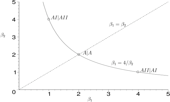
Figure 1: Curves in the $(\beta_{1},\beta_{2})$ plane for which we construct solutions. The group theoretical points are also indicated.

of the models introduced in Sections III.1 and III.2.

In Sections IV.1 and IV.2 we state and discuss the solutions on the diagonal and on the hyperbola, respectively. The solutions we derive on the hyperbola are generalizations of the recursion formula stated in Section II.2. In Section IV.3 we give the derivation. We also present some few–particle solutions in Section IV.4.

IV.1 Solutions on the Diagonal $\beta=\beta_{1}=\beta_{2}$

In this case the Schrödinger equation is Eq. (15). It decouples into equations for two independent sets of particles. Hence we can write the solution as the product

$$\eta_{k_{1}k_{2}}^{(\beta)}(s,r)=\Psi_{k_{1}}^{(\beta)}(s_{1},r_{1})\ \Psi_{k_{2}}^{(\beta)}(s_{2},r_{2})\ .$$ (35)

An explicit expression of $\Psi_{k_{i}}^{(\beta)}(s_{i},r_{i}),\ i=1,2$ can be obtain in terms of the recursion formula Eq. (6) and (7) in combination with Eq. (4). We point out that the calculation of each $\Psi_{k_{i}}^{(\beta)}(s_{i},r_{i})$ separately is in itself very difficult.

IV.2 Solutions on the Hyperbola $\beta=\beta_{2}=4/\beta_{1}$

In general, the interaction term between the two different sets of one–dimensional particles at positions $s_{p1}$ and $s_{q2}$ in the superunitary model (26) does not vanish. Thus, as the product form of Eq. (35) is destroyed, it is highly non–trivial to obtain solutions for positive parameters $\beta_{1}$ and $\beta_{2}$ and for arbitrary dimensions $k_{1}$ and $k_{2}$. Nevertheless, we derive solutions on the hyperbola $\beta_{2}=4/\beta_{1}$ shown in Fig. 1. On this hyperbola, the exponent in the denominator of the function (22) has the constant value two. Exactly on the same hyperbola $\beta_{2}=4/\beta_{1}$, Sergeev and Veselov constructed supersymmetric extensions of CMS models and their solutions in terms of deformed Jack polynomials serves1 ; serves2 . The existence of a recursion formula suggests that there should be a recursion formula akin to the formula derived by Okounkov and Olshanski OO for the deformed Jack polynomials as well.

We emphasize again that we expect the superunitary model (26) to be exactly solvable for any positive $\beta_{1}$,$\beta_{2}$.

As argued in Refs. GUKOP1 ; GUKO1 , the recursion formulae (6) can be viewed as generating functions for Jack polynomials, or equivalently, as a proper resummation. This carries over to the present case. We generalize the supersymmetric recursion formula of Ref. GUKO2 for the symmetric superspace ${\rm AI|AII}$ discussed in Section III.4. We analytically continue the solution at the point $(\beta_{1},\beta_{2})=(1,4)$, $(4,1)$ and $(2,2)$. Thereby we construct the solution on the hyperbola.

We write $\rho_{k_{1}k_{2}}^{(c,\beta)}=\rho_{k_{1}k_{2}}^{(c,4/\beta,\beta)}$ for the solution of the superunitary model (24) on the hyperbola. In Section IV.3 it will be proved that $\rho_{k_{1}k_{2}}^{(c,\beta)}$ can be expressed through the recursion formula

$$\rho_{k_{1}k_{2}}^{(c,\beta)}(s_{1},s_{2},r_{1},r_{2})\ =\int d\mu^{(c,\beta)}(s^{\prime},s)\exp\left(i\left(\sum_{p=1}^{k_{1}}s_{p1}-\sum_{p=1}^{k_{1}-1}s_{p1}^{\prime}+\frac{\beta}{2}\sum_{p=1}^{k_{2}}|\xi_{p}|^{2}\right)r_{k_{1}1}\right)\,\rho_{(k_{1}-1)k_{2}}^{(c,\beta)}(s^{\prime},\widetilde{r})\quad.$$ (36)

Here, $\rho_{(k_{1}-1)k_{2}}^{(c,\beta)}(s^{\prime},\widetilde{r})$ is the solution of the superunitary model (24) for the $k_{1}+k_{2}-1$ variables $s^{\prime}=(s^{\prime}_{11},\ldots,s^{\prime}_{(k_{1}-1)1},s^{\prime}_{12},\ldots,s^{\prime}_{k_{2}2})$. The solution is labeled by the quantum numbers $\widetilde{r}=(r_{11},\ldots,r_{(k_{1}-1)1},r_{12},\ldots,r_{k_{2}2})$. The primed variables are the integration variables. The integration variables $s_{p1}$ are commuting. Their domain of integration is compact and given by

$$s_{p1}\ \leq\ s_{p1}^{\prime}\ \leq\ s_{(p+1)1}\ ,\qquad p=1,\ldots,(k_{1}-1)\ .$$ (37)

The integration variables $s_{p2}^{\prime}$ are related to Grassmann variables $\xi_{p}$ and $\xi_{p}^{*}$ by

$$|\xi_{p}|^{2}\ =\ cs_{p2}^{\prime}-cs_{p2}\ .$$ (38)

The modulus squared of a Grassmann variable is defined by

$$|\xi_{p}|^{2}\ =\ \xi_{p}^{*}\xi_{p}\ =-\ \xi_{p}\xi_{p}^{*}\ ,$$ (39)

which is the formal analogue for the length squared of a commuting variable. The integration over Grassmann variables is defined by

$$\int d\xi_{p}d\xi_{p}^{*}=0\quad{\rm and}\quad\int|\xi_{p}|^{2}d\xi_{p}d\xi_{p}^{*}=1\ .$$ (40)

The normalization to one differs from the convention we used in Ref. GUKO2 , where the integral was normalized to $1/2\pi$. The integration measure $d\mu^{(c,\beta)}(s^{\prime},s)$ reads

$$d\mu^{(c,\beta)}(s^{\prime},s) = \mu^{(c,\beta)}(s^{\prime},s)d[\xi]d[s_{1}^{\prime}]$$

$$\mu^{(c,\beta)}(s^{\prime},s) = \mu_{B}^{(\beta)}(s_{1}^{\prime},s_{1})\mu_{F}^{(c,\beta)}(s_{2}^{\prime},s_{2})\mu_{BF}^{(c,\beta)}(s^{\prime},s)\ ,$$ (41)

with the products of the differentials

$$d[\xi]=\prod_{p=1}^{k_{2}}d\xi_{p}d\xi_{p}^{*}\quad{\rm and}\quad d[s_{1}^{\prime}]=\prod_{p=1}^{k_{1}-1}ds_{p1}^{\prime}\ ,$$ (42)

and the measure functions

$$\mu_{B}^{(\beta)}(s_{1}^{\prime},s_{1}) = \Delta_{k_{1}}(s_{1}^{\prime})\Delta_{k_{1}}^{1-4/\beta}(s_{1})\left(-\prod_{p,q}\left(s_{p1}-s_{q1}^{\prime}\right)\right)^{2/\beta-1}$$

$$\mu_{F}^{(c,\beta)}(s_{2}^{\prime},s_{2}) = \Delta_{k_{2}}^{\beta^{2}/4}(cs_{2}^{\prime})\Delta_{k_{2}}^{\beta^{2}/4-\beta}(cs_{2})\prod_{p\neq q}^{k_{2}}(cs_{p2}-cs_{q2}^{\prime})^{\beta/2-\beta^{2}/4}$$

$$\mu_{BF}^{(c,\beta)}(s^{\prime},s) = \prod_{p=1}^{k_{1}}\prod_{l=1}^{k_{2}}\prod_{q=1}^{k_{1}-1}(cs_{l2}-s_{p1})^{2-\beta/2}(cs_{l2}-s_{q1}^{\prime})^{\beta/2-1}(cs_{l2}^{\prime}-s_{p1})^{\beta/2-1}(cs_{l2}^{\prime}-s_{q1}^{\prime})^{-\beta/2}\ .$$ (43)

We split the measure function into three parts $\mu_{B},\ \mu_{F},\ \mu_{BF}$ as in Ref. GUKO2 . We do so, because the coordinates are originally, for certain values of $\beta_{1}$ and $\beta_{2}$, Bosonic and Fermionic eigenvalues of some supermatrices. The recursion formula (36) reproduces the recursion formula derived in Refs. GUKOP2 ; GUKO2 for $\beta=4$. It also reproduces the supersymmetric Harish–Chandra integral discussed in Ref. GGT for $\beta=2$. Moreover, for $k_{2}=0$ the recursion formula in ordinary space found in Refs. GUKOP1 ; GUKO1 and briefly discussed in Section II.2 is naturally recovered.

The case $k_{1}=0$ deserves some special attention, because $\mu_{B}$ and $\mu_{BF}$ vanish and so does the exponential in Eq. (36). Importantly, the function $\mu_{F}$ does not. The corresponding Schrödinger equation is just that of the CMS–Hamiltonian for $k_{2}$ particles as defined in Eq. (5). Its solution, or more precisely the solution of its associated Laplace equation (1), is by definition given by $\rho_{0k_{2}}^{(c,\beta)}=\Phi_{k_{2}}^{(\beta)}$. However, the recursion formula yields another solution

$$\widetilde{\Phi}_{k_{2}}^{(\beta)}(s_{2},r_{2})=\int d[\xi]\mu_{F}(s_{2},s_{2}^{\prime})\Phi_{k_{2}}^{(\beta)}(s^{\prime}_{2},r_{2})\ .$$ (44)

For this to hold the Laplacean $\Delta_{s_{2}}^{(\beta)}$ defined in Eq. (2) has to commute with the Grassmann integration of Eq. (44). This implies that the eigenvalues of the operator defined through the Grassmann integration are conserved quantities. Indeed, the operator $\Delta_{s_{2}}^{(\beta)}$ commutes with the Grassmann integral Eq. (44),

$$\Delta_{s_{2}}^{(\beta)}\int d[\xi]\mu_{F}(s_{2},s_{2}^{\prime})f(s^{\prime}_{2})=\int d[\xi]\mu_{F}(s_{2},s_{2}^{\prime})\Delta_{s^{\prime}_{2}}^{(\beta)}f(s^{\prime}_{2})\ ,$$ (45)

where $f(s^{\prime}_{2})$ is analytic and symmetric in its arguments, but otherwise an arbitrary test function. We sketch the derivation of Eq. (45) in A.

IV.3 Proof of the Recursion Formula

We now prove that the functions $\rho_{k_{1}k_{2}}^{(c,\beta)}$ given by Eq. (36) indeed solve the differential equation Eq. (23) on the hyperbola. The proof relies on the invariance properties of the measure function $\mu^{(c,\beta)}(s^{\prime},s)$. We define the Laplace operator Eq. (23) on the hyperbola $\Delta_{s}^{(c,\beta)}=\Delta_{s}^{(c,4/\beta,\beta)}$ and the center of mass momentum operator

$$P_{s}^{(c)}=\sum_{p=1}^{k_{1}}\frac{\partial}{\partial s_{p1}}-c\sum_{p=1}^{k_{2}}\frac{\partial}{\partial s_{p2}}\ .$$ (46)

We then have the two identities

$$P_{s}^{(c)}\int d\mu(s,s^{\prime})f(s_{1}^{\prime},s_{2}^{\prime}) = \int d\mu(s,s^{\prime})P_{s^{\prime}}^{(c)}f(s_{1}^{\prime},s_{2}^{\prime})$$

$$\Delta_{s}^{(c,\beta)}\int d\mu(s,s^{\prime})f(s^{\prime}_{1},s^{\prime}_{2}) = \int d\mu(s,s^{\prime})\Delta_{s^{\prime}}^{(c,\beta)}f(s_{1}^{\prime},s_{2}^{\prime})\ ,$$ (47)

which hold for an arbitrary function $f(s_{1},s_{2})$ symmetric in both sets of arguments $s_{p1},\ p=1\ldots k_{1}$ and $s_{p2},\ p=1\ldots k_{2}$. We derive Eqs. (47) by direct calculation, using repeated integration by part. This procedure is relatively simple for the first equation of (47). However, for the second one it becomes rather tedious due to the complexity of the measure function. Some of the steps are sketched in B. A more elegant proof is likely to exist.

Employing the properties (47), we can now prove the recursion formula by acting from the left with $\Delta_{s}^{(c,\beta)}$ on both sides of Eq. (36). We set

$$f(s_{1}^{\prime},s_{2}^{\prime})=\exp\left(-i\left(\sum_{p=1}^{k_{1}-1}s_{p1}^{\prime}-\frac{\beta}{2}\sum_{p=1}^{k_{2}}is_{p2}^{\prime}\right)r_{k_{1}1}\right)\,\rho_{(k_{1}-1)k_{2}}^{(c,\beta)}(s^{\prime},\widetilde{r})\ ,$$ (48)

and obtain straightforwardly from (47)

$$\Delta_{s}^{(c,\beta)}\rho_{k_{1}k_{2}}^{(c,\beta)}(s,r)\ =\int d\mu^{(c,\beta)}(s^{\prime},s)\exp\left[i\left(\sum_{p=1}^{k_{1}}s_{p1}-\sum_{p=1}^{k_{1}-1}s_{p1}^{\prime}+\frac{\beta}{2}\sum_{p=1}^{k_{2}}|\xi_{p}|^{2}\right)r_{k_{1}1}\right]$$

$$\qquad\qquad\qquad\qquad\left(-\frac{\sqrt{\beta}}{2}r_{k_{1}1}^{2}+\Delta_{s^{\prime}}^{(c,\beta)}\right)\rho_{(k_{1}-1)k_{2}}^{(c,\beta)}(s^{\prime},\widetilde{r})\ .$$ (49)

Since by definition we have

$$\Delta_{s^{\prime}}^{(c,\beta)}\rho_{(k_{1}-1)k_{2}}^{(c,\beta)}(s^{\prime},\widetilde{r})=-\left(\sum_{p=1}^{k_{1}-1}\frac{\sqrt{\beta}}{2}r_{p1}^{2}+\sum_{p=1}^{k_{2}}\frac{r_{p2}^{2}}{\sqrt{\beta}}\right)\rho_{(k_{1}-1)k_{2}}^{(c,\beta)}(s^{\prime},\widetilde{r})\ ,$$ (50)

we arrive at

$$\Delta_{s}^{(c,\beta)}\rho_{k_{1}k_{2}}^{(c,\beta)}(s,r)=-\left(\sum_{p=1}^{k_{1}}\frac{\sqrt{\beta}}{2}r_{p1}^{2}+\sum_{p=1}^{k_{2}}\frac{r_{p2}^{2}}{\sqrt{\beta}}\right)\rho_{k_{1}k_{2}}^{(c,\beta)}(s,r)\ ,$$ (51)

which is our assertion.

IV.4 Few Particle Solutions

Once the eigenfunction $\Phi_{k_{2}}^{(c,\beta)}(s_{2},r_{2})$ in ordinary space is known, we can recursively construct the eigenfunctions $\rho_{k_{1}k_{2}}^{(c,\beta)}(s,r)$ from formula (36) by starting with $\rho_{0k_{2}}^{(c,\beta)}(s,r)=\Phi_{k_{2}}^{(c,\beta)}(s_{2},r_{2})$. The eigenfunctions $\Phi_{k_{2}}^{(c,\beta)}(s_{2},r_{2})$ are given by the recursion formula in ordinary space, see Section II.2. We illustrate the procedure for two examples in superspace. For the sake of simplicity, we consider only $c=+i$ and suppress the upper index $(c)$ in the sequel.

To begin with, we study the case $k_{1}=k_{2}=1$. The eigenvalue equation is

$$\left[\frac{1}{\sqrt{\beta_{1}}}\frac{\partial^{2}}{\partial s_{11}^{2}}+\frac{1}{\sqrt{\beta_{2}}}\frac{\partial^{2}}{\partial s_{12}^{2}}-\frac{1}{s_{11}-is_{12}}\left(\sqrt{\beta_{1}}\frac{\partial}{\partial s_{11}}+i\sqrt{\beta_{2}}\frac{\partial}{\partial s_{21}}\right)\right]\rho_{11}^{(\beta_{1},\beta_{2})}(s,r)\ =\$$

$$\qquad\qquad\qquad\qquad\qquad\qquad\qquad\qquad\qquad\qquad\qquad\qquad-\left(\frac{r_{11}^{2}}{\sqrt{\beta_{1}}}+\frac{r_{12}^{2}}{\sqrt{\beta_{2}}}\right)\rho_{11}^{(\beta_{1},\beta_{2})}(s,r)$$ (52)

yielding the closed solution

$$\rho_{11}^{(\beta_{1},\beta_{2})}(s,r) = \exp\left[\pm\frac{i}{\sqrt{\beta_{1}}-\sqrt{\beta_{2}}}\left(\sqrt{\beta_{1}}s_{11}-i\sqrt{\beta_{2}}s_{12}\right)\left(r_{11}-ir_{12}\right)\right]|\sqrt{\beta_{1}}-\sqrt{\beta_{2}}|^{\sqrt{\beta_{1}\beta_{2}}/2}z^{\nu}{\bf H}^{\mp}_{\nu}(z)\ .$$ (53)

Here, ${\bf H}_{\nu}(z)$ is the Hankel function of order $\nu=\sqrt{\beta_{1}\beta_{2}/4}+1/2$. Its argument is the dimensionless complex variable

$$z=\frac{\sqrt{\beta_{2}}r_{11}-i\sqrt{\beta_{1}}r_{12}}{\sqrt{\beta_{2}}-\sqrt{\beta_{1}}}\left(s_{11}-is_{12}\right)\ .$$ (54)

The result (53) holds for all arbitrary positive parameters $\beta_{1}$ and $\beta_{2}$.

From Eq. (53) we can gain deeper insight into the structure of the solutions on the hyperbola $\beta_{1}\beta_{2}=4$. The order $\nu$ of the Hankel function becomes $3/2$ on the hyperbola. The asymptotic Hankel series of the half integer Hankel function of order $n+1/2$ terminates after the $n$–th step ABR . On the other hand, the asymptotic series of a Hankel function whose order is not half–integer is infinite. Thus, only the Hankel functions of half–integer order can be expressed as a product of a finite polynomial and an exponential. The value $\nu=1/2$ corresponds to either $\beta_{1}=0$ or $\beta_{2}=0$ and hence to a one–type–of–particle model, see Eq. (1) and Eq. (5). Consequently, the order $\nu=3/2$ is the lowest half integer order describing a two–type–particle model that has a non–trivial solution which can be written as product of a polynomial and an exponential. Furthermore, we notice that it is exactly this extra term in the Hankel expansion of ${\bf H}^{\mp}_{3/2}(z)$ which can be expressed by an integration over properly chosen Grassmann variables. Indeed the recursion formula yields directly

$$\rho_{11}^{(\beta)}\left(s_{11},s_{12},r_{11},\beta r_{12}/2\right)=\exp\left(ir_{11}s_{11}+i\beta r_{12}s_{12}/2\right)\left[\left(\frac{\beta}{2}-1\right)+\frac{i\beta}{2}\left(is_{12}-s_{11}\right)\left(ir_{12}-r_{11}\right)\right]\ ,$$ (55)

which is identical to Eq. (53) on the hyperbola. We expect recursive solutions of the $k_{1}+k_{2}$ particle Hamiltonian Eq. (26) akin to the recursion formula Eq. (36) to exist for other half–integer $\nu$ as well.

The next simplest case is $k_{1}=1$ and $k_{2}=2$ and vice versa. It is still possible although cumbersome to find an exact solution for arbitrary $\beta_{1}$ and $\beta_{2}$. As we only wish to illustrate how the recursion works, we do not derive this exact solution here. Rather we use formula (36) to find a solution on the hyperbola. Without loss of generality we choose $k_{2}=2$ and $k_{1}=1$. The bosonic measure $\mu_{B}(s_{1},s_{1}^{\prime})$ vanishes. We have only to perform four Grassmann integrations. This implies that the solution can be written as a differential operator acting on $\rho_{02}^{(c,\beta)}(s_{2},\beta r_{2}/2)=\Phi_{2}^{(\beta)}(s_{2},\beta r_{2}/2)$

$$\rho_{12}^{(\beta)}(s_{1},s_{2},r_{1},\beta r_{2}/2)=L^{(\beta)}(s,r)\Phi_{2}^{(\beta)}(s_{2},\beta r_{2}/2)\ .$$ (56)

Using the definitions of the measure Eq. (41) and Eq. (43) and doing the Grassmann integrations we find

$$L^{(\beta)}(s,r) = \prod_{p=1}^{2}\left(is_{p2}-s_{11}\right)\left\{\prod_{q=1}^{2}\left[\left(\frac{\beta}{2}-1\right)\frac{1}{is_{q2}-s_{11}}+i\frac{\beta}{2}r_{11}-i\frac{\partial}{\partial s_{q2}}\right]\right.$$ (57)

$$\quad\left.+\frac{\beta}{2}\left(\frac{\beta}{2}-1\right)\frac{1}{\prod_{p=1}^{2}\left(is_{p2}-s_{11}\right)}+\frac{\beta}{2}\frac{1}{\left(s_{12}-s_{22}\right)}\left(\frac{\partial}{\partial s_{12}}-\frac{\partial}{\partial s_{11}}\right)\right\}\ .$$

For the eigenfunction $\Phi_{2}^{(\beta)}(s_{2},\beta r_{2}/2)$, we employ the explicit form GUKOP1 ; GUKO1

$$\Phi_{2}^{(\beta)}(s_{2},\beta r_{2}/2)\ =\ \exp\left(-i\beta\frac{(s_{12}+s_{22})(r_{12}+r_{22})}{4}\right)\,\chi^{(\beta+1)}\left(\frac{\beta z}{4}\right)$$ (58)

which involves the spherical functions

$$\chi^{(\beta+1)}(w)=2^{(\beta-1)/2}\Gamma((\beta+1)/2)\frac{J_{(\beta-1)/2}(w)}{w^{(\beta-1)/2}}\ ,$$ (59)

where $J_{\nu}$ is the Bessel function of order $\nu$. The variable $z=(s_{12}-s_{22})(r_{12}-r_{22})$ in Eq. (58) is dimensionless. Plugging this expression into Eq. (56) and using Eq. (57) we can cast $\rho_{12}^{(\beta)}$ into the form

$$\rho_{12}^{(\beta)}\left(s_{11},s_{2},r_{11},\beta r_{2}/2\right) = \exp\left(ir_{11}s_{11}+\frac{\beta}{4}i\left(r_{12}+r_{22}\right)\left(s_{12}+s_{22}\right)\right)$$ (60)

$$\left\{\left(\frac{\beta}{2}-1\right)\left[\beta-1+2z\frac{d}{dz}+i\frac{\beta}{2}\left(r_{11}-\frac{ir_{12}}{2}-\frac{ir_{22}}{2}\right)\left(s_{11}-\frac{is_{12}}{2}-\frac{is_{22}}{2}\right)\right]\right.$$

$$\qquad\left.-\frac{\beta^{2}}{4}\prod_{p=1}^{2}(r_{11}-ir_{p2})(s_{11}-is_{p2})\right\}\chi^{(\beta+1)}\left(\beta z/4\right)\ ,$$

which explicitly shows the symmetry between the two sets of arguments $s$ and $r$.

V Physical Interpretation

To develop an intuition for the physics of the differential operators (26) and (34) in superspace, we recall the physical interpretation of CMS models in ordinary space. The Schrödinger equation (5) models a system of $N$ interacting particles in one dimension, moving on the $x$–axis, say. The eigenfunctions are labeled by a set of conserved quantities or, equivalently, quantum numbers $k_{n},\ n=1\ldots N$. This is tantamount to saying that the system is exactly solvable. In the limit of vanishing coupling, i.e. for $\beta=2$, the quantum numbers are the momenta of each particle. The characteristic feature of this model is the $(x_{n}-x_{m})^{-2}$ interaction potential. The models based on the ordinary groups ${\rm O}(N)$ and ${\rm Sp}(2N)$ fit into the same picture. However, the models have in this case a symmetry under point reflections about $x=0$. Moreover, for the symplectic group and the orthogonal group with $N$ odd, there is an additional inverse quadratic confining or deconfining central potential OP .

We now show that the physical interpretation along those lines carries over to our superspace models in a most natural way. We discuss the superunitary model in Section V.1 and the orthosymplectic model in Section V.2.

V.1 Superunitary Model

The superunitary model is given by Eq. (26). We notice that its differential operator is not Hermitean. This leads to some ambiguity in the interpretation of the model. The imaginary unit in the parameter $c$ is due to a Wick–type–of rotation of the variables $s_{p2}$. This was needed in Ref. EFE83 to ensure convergence of integrals over certain supermatrices. However, in our application, there is no such convergence problem, as long as we do not go into a thermodynamical discussion of the model. Thus, we undo the Wick rotation by the substitution $is_{p2}\rightarrow s_{p2},\ p=1\ldots k_{2}$. We introduce the coupling constants

$$g_{11} = \sqrt{\beta_{1}}\left(\frac{\beta_{1}}{2}-1\right)$$

$$g_{22} = \sqrt{\beta_{2}}\left(\frac{\beta_{2}}{2}-1\right)$$

$$g_{12} = \frac{1}{2}\left(\sqrt{\beta_{1}}-\sqrt{\beta_{2}}\right)\left(\frac{1}{2}\sqrt{\beta_{1}\beta_{2}}+1\right)$$ (61)

and the masses

$$m_{1}=\sqrt{\beta_{1}/4}\quad{\rm and}\quad m_{2}=-\sqrt{\beta_{2}/4}\ .$$ (62)

We notice that the mass $m_{1}$ is positive, while the mass $m_{2}$ is negative. Introducing the momenta $\pi_{p1}=-i\partial/\partial s_{p1}$ and $\pi_{p2}=-i\partial/\partial s_{p2}$, we eventually obtain the Hermitean Hamiltonian

$$H = \sum_{p=1}^{k_{1}}\frac{\pi_{p1}^{2}}{2m_{1}}+\sum_{p=1}^{k_{2}}\frac{\pi_{p2}^{2}}{2m_{2}}+\sum_{p<q}\frac{g_{11}}{\left(s_{p1}-s_{q1}\right)^{2}}-\sum_{p<q}\frac{g_{22}}{\left(s_{p2}-s_{q2}\right)^{2}}-\sum_{p,q}\frac{g_{12}}{(s_{p1}-s_{q2})^{2}}\ ,$$ (63)

with now canonical conjugate variables, $[s_{ql},\pi_{pj}]=i\delta_{pq}\delta_{jl}$. In second quantized form it reads

$$H = \sum_{i}\int dx\frac{1}{2m_{i}}\psi_{i}^{\dagger}(x)\nabla^{2}\psi_{i}(x)+\sum_{i,j}\int dxdx^{\prime}\frac{g_{ij}}{(x-x^{\prime})^{2}}\psi_{i}^{\dagger}(x)\psi_{j}^{\dagger}(x^{\prime})\psi_{j}(x^{\prime})\psi_{i}(x)\ .$$ (64)

The Hamiltonian (63) describes a one–dimensional interacting many–body system for two kinds of $k_{1}$ particles at positions $s_{p1},\ p=1,\ldots,k_{1}$ and $k_{2}$ particles at positions $s_{p2},\ p=1,\ldots,k_{2}$ on the $s$ axis.

The superunitary model in the form (63) may be employed to describe electrons in a quasi–one–dimensional semiconductor, see Fig. 2. The electrons are subject to a periodic

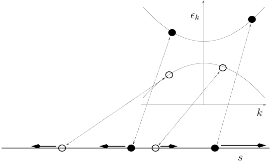
Figure 2: Electrons in the upper (black circles) and lower (open circles) band of a quasi–one–dimensional semiconductor. The dispersion relations $\epsilon_{k}$ as function of the wave number $k$ are indicated by the parabola and the inverted parabola. The particles are then mapped onto the $s$ axis in the bottom part.

potential. There is an upper and a lower band, separated by a gap. The electrons in the upper band have a positive (effective) mass, while the electrons in the lower band close to the gap have a negative (effective) mass. This is due to the dispersion relation $\epsilon_{k}$ as function of the wave number $k$. Its second derivative, i.e. the inverse mass, is positive in the upper, but negative in the lower band KIT . We recall that the coupling constants $g_{ij}$ are not arbitrary, they are functions of both $\beta_{1}$ and $\beta_{2}$. This makes it possible to model repulsive as well as attractive interactions between equal particles and also between different particles by choosing proper parameters $\beta_{1}$ and $\beta_{2}$. We mention that the spectrum has to be bound from below by an additional mechanism if one wants to derive thermodynamical quantities.

V.2 Orthosymplectic Model

As the orthosymplectic model (34) is derived from the symmetric superspace ${\rm OSp}$ $(k_{1}/2k_{2})$, it has additional symmetries, comprising the ones found in the models based on the ordinary groups ${\rm O}$$(N)$ and ${\rm Sp}$$(2N)$. There is a symmetry of point reflections about $s_{1}=0$ and about $s_{2}=0$. This renders the differential operator of the orthosymplectic model (34) real and thus Hermitean as it stands. It describes a quasi–two–dimensional physical system. One set of particles at positions $s_{p1}$ is confined to the $s_{1}$ axis and a second set of particles at positions $s_{p2}$ confined to the orthogonal $s_{2}$ axis. As in the superunitary model, all particles interact through a distance dependent, inverse quadratic potential. The point reflection symmetry about the two axes implies that each particle at the position $s_{pj}$ $>0$ with the momentum $\pi_{pj}$ has a counterpart at the position $-s_{i1}$ with the momentum $-\pi_{pj}$. Moreover, due to the reflection symmetry, the particles are also subjected to a confining or deconfining inverse quadratic central potential. This generalizes the situation described by the models from the ordinary groups ${\rm O}(N)$ and ${\rm Sp}(N)$ OP .

However, the orthosymplectic model has yet another important feature. Closer inspection reveals that the potentials also contain angular dependent terms. We now show that these are dipole–dipole interactions, referred to as tensor forces in nuclear physics BOMO1 . The general form of such a dipole–dipole interaction in $d$ dimensions reads

$$V({\vec{r}}_{p},{\vec{r}}_{q})=v(|{\vec{r}}_{p}-{\vec{r}}_{q}|)\left(({\vec{e}}_{pq}\cdot{\vec{\sigma}_{p}})({\vec{e}}_{pq}\cdot{\vec{\sigma}_{q}})-\frac{1}{d}{\vec{\sigma}_{p}}\cdot{\vec{\sigma}_{q}}\right)\ ,$$ (65)

where ${\vec{r}}_{p}$ is the position of particle $p$ and ${\vec{\sigma}_{p}}$ the dipole vector attached to it. The vector ${\vec{e}}_{pq}$ is the unit vector pointing in the direction ${\vec{r}}_{p}-{\vec{r}}_{q}$. The potential $v(r)$ depends on the distance between the particles only. In nuclear physics, it is short–ranged BOMO1 , in our case the potential comes out inverse quadratic, $v(r)=1/r^{2}$. In the following discussion we assume $d=2$. This assumption is not a necessary one. Interpretations in higher dimensions are also possible, but may be discussed elsewhere. We notice that the functional form of the potential, when derived from a Poisson equation, depends on the number of spatial dimensions. Thus, one should not view the dipole–dipole interaction as stemming from a Coulomb potential in the present two–dimensional interpretation. For $d=2$ we write Eq. (65) more explicitly as

$$V({\vec{r}}_{p},{\vec{r}}_{q})=\frac{\sigma_{p}\sigma_{q}}{|{\vec{r}}_{p}-{\vec{r}}_{q}|^{2}}{\vec{e}}_{pq}^{\ T}\left[\matrix{\cos(\vartheta_{p}+\vartheta_{q})&\cos\vartheta_{p}\sin\vartheta_{q}\cr\sin\vartheta_{p}\cos\vartheta_{q}&-\cos(\vartheta_{p}+\vartheta_{q})}\right]{\vec{e}}_{pq}\ .$$ (66)

with ${\vec{\sigma}}_{p}=\sigma_{p}(\cos\vartheta_{p},\sin\vartheta_{p})$. In our quasi–two–dimensional model, there are three possibilities for the distance vectors ${\vec{r}}_{p}-{\vec{r}}_{q}$. Expressed in the coordinates $s_{p1}$ and $s_{p2}$, they read

$${\vec{r}}_{p}-{\vec{r}}_{q}=\left[\matrix{\pm s_{p1}\pm s_{q1}\cr 0}\right]\ ,\ \left[\matrix{0\cr\pm s_{p2}\pm s_{q2}}\right]\ ,\ \left[\matrix{\pm s_{p1}\cr\pm s_{q2}}\right]\ ,$$ (67)

depending on which axis the particles $p$ and $q$ move. The angular dependent interaction in Eq. (34) can easily be cast into the form (66).

Hence, the orthosymplectic model (34) describes the motion of two kinds of charged particles with dipole vectors attached to them. The interaction comprises, first, a central potential, second, an only distance dependent potential and third a tensor force. Two examples are sketched in Fig. 3.

Figure 3: Two realizations of the orthosymplectic model. Left: $2k_{1}=4$ particles on the $s_{1}$ axis and $2k_{2}=6$ particles on the $s_{2}$ axis. The dipole vectors on the same axis have the same direction. Tensor forces are indicated as thicker and thinner dashed lines, corresponding to the strength of the force. The central forces and the distance dependent forces are not depicted. Right: a case with different directions of the dipole vectors on different sides of the same axis.

Restricting ourselves to even $k_{1}$, we cast the Hamiltonian into the new form

$$2H = \sum_{p=1}^{k_{1}}\frac{\pi_{p1}^{2}}{2m_{1}}+\sum_{p=1}^{2k_{2}}\frac{\pi_{p2}^{2}}{2m_{2}}+\sum_{p\neq q}\frac{h_{11}}{\left(s_{p1}-s_{q1}\right)^{2}}+\sum_{p<q}\frac{h_{22}}{\left(s_{p2}-s_{q2}\right)^{2}}$$ (68)

$$-\sum_{p,q}\frac{h_{12}}{s_{p1}^{2}+s_{q2}^{2}}+\sum_{p=1}^{k_{1}}\frac{f_{1}}{s_{p1}^{2}}+\sum_{p=1}^{2k_{2}}\frac{f_{2}}{s_{p2}^{2}}+\sum_{p,q}\frac{\left({\vec{e}}_{pq}\cdot{\vec{\sigma}_{1}}\right)\left({\vec{e}}_{pq}\cdot{\vec{\sigma}_{2}}\right)-{\vec{\sigma}_{1}}\cdot{\vec{\sigma}_{2}}/2}{s_{p1}^{2}+s_{q2}^{2}}\ ,$$

and match it on Eq. (34) by adjusting the parameters. The masses are uniquely determined. They are now both positive and given by

$$m_{1}=\sqrt{\beta_{1}/4}\quad{\rm and}\quad m_{2}=\sqrt{\beta_{2}/4}\ .$$ (69)

In order to determine the other free parameters in Eq. (68) we have to choose specific directions of the dipoles. There are various constraints. All dipoles attached to the particles on the negative $s_{1}$ axis must point into the same direction, described by the angle $\vartheta_{1-}$, say. Similar constraints apply to the dipoles on the other half–axes. We denote the corresponding angles by $\vartheta_{1+}$ for the positive $s_{1}$ axis and with $\vartheta_{2-}$ and $\vartheta_{2+}$ for the half–axes in $s_{2}$ direction. Nevertheless, the four angles can not be chosen arbitrarily, there are some further constraints which are given in C, together with a complete list of all possible combinations of different directions. Here we only consider the possibility $\vartheta_{1-}=\vartheta_{1+}=\vartheta_{1}$ and $\vartheta_{2-}=\vartheta_{2+}=\vartheta_{2}$. Moreover, there is some arbitrariness for choosing the moduli $\sigma_{j},\ j=1,2$. For the sake of simplicity, we assume the strengths of both dipoles to be the same $\sigma_{1}=\sigma_{2}=\sigma$.

The strength of the central potential in the Hamiltonian (68) is given by

$$f_{1}=\frac{\beta_{1}}{8}\left(\frac{\beta_{1}}{2}-1\right)\quad{\rm and}\quad f_{2} = -\frac{\beta_{2}}{8}\left(\frac{\beta_{2}}{2}-1\right)\ .$$ (70)

When trying to determine the coupling constants $h_{ij}$ in the Hamiltonian (68), we face yet another type of arbitrariness. There are at least two possibilities. The tensor force could, first, act between pairs of particles one on either axis or it could, second, acts between all particles. We choose the second option as it seems more natural. The coupling constants are then given by

$$h_{11} = \sqrt{\beta_{1}}\left(\frac{\beta_{1}}{2}-1\right)+\sigma^{2}\cos 2\vartheta_{1}$$

$$h_{22} = \sqrt{\beta_{2}}\left(\frac{\beta_{2}}{2}-1\right)+\sigma^{2}\cos 2\vartheta_{2}$$

$$h_{12} = \frac{\sqrt{\beta_{1}\beta_{2}}}{4}\left(\sqrt{\beta_{1}}-\sqrt{\beta_{2}}\right)\ .$$ (71)

The strength of the dipoles is determined through the relation

$$\sigma^{2}\cos(\vartheta_{1}+\vartheta_{2})=2\left(1+\frac{1}{2}\sqrt{\beta_{1}\beta_{2}}\right)\left(\sqrt{\beta_{1}}-\sqrt{\beta_{2}}\right)\ .$$ (72)

A sketch of two possible realizations is given in Fig. 3. Notice that the tensor force between two dipoles vanishes at a relative angle of $45^{\circ}$ between the particle positions.

Of course $H$ in Eq. (68) and the operator $\widetilde{H}$, say, on the left hand side of Eq. (34) are still not identical. For $H$ and $\widetilde{H}$ to be equivalent, the time evolution for the many–body wavefunction $\psi_{k_{1},k_{2}}^{(\beta_{1},\beta_{2})}(s,t)$ has to be the same. Thus, the corresponding time dependent Schrödinger equations have to fulfill

$$i\frac{\partial}{\partial t}\psi_{k_{1},k_{2}}^{(\beta_{1},\beta_{2})}(s,t)\ =\ H\psi_{k_{1}k_{2}}^{(\beta_{1},\beta_{2})}(s,t)\ =\ \widetilde{H}\psi_{k_{1}k_{2}}^{(\beta_{1},\beta_{2})}(s,t)\ .$$ (73)

Thus, the wave function at $t=0$ must already have the reflection symmetry

$$\psi_{k_{1},k_{2}}^{(\beta_{1},\beta_{2})}(s,0)=\psi_{k_{1},k_{2}}^{(\beta_{1},\beta_{2})}(-s,0)\qquad{\rm at}\quad t=0\ .$$ (74)

The different interaction strengths are sketched by different widths of the interaction lines. In C, all possible combinations of the dipole directions are derived. They are shown in Fig. 4.

Figure 4: Panel of the possible dipole directions in the orthosymplectic model as derived C.

Apart from some sign changes, all formulae given above for the coupling constants are valid for odd $k_{1}$ as well.

VI Summary and Conclusions

Using supersymmetry, we derived new classes of models for interacting particles. We obtained, first, a superunitary model which is based on the supergroup ${\rm GL}(k_{1}/k_{2})$ and on the symmetric superspace ${\rm GL}(k_{1}/2k_{2})/{\rm OSp}(k_{1}/2k_{2})$ and, second, an orthosymplectic model which is based on the supergroup ${\rm OSp}(k_{1}/2k_{2})$. It is crucial that these models depend in a non–trivial way on two real parameters $\beta_{1}$ and $\beta_{2}$. Our models extend and include the models of the CMS type in ordinary space.

Moreover, our superunitary model contains the supersymmetric constructions derived in Refs. serves1 ; serves2 . The latter depend on one parameter only, implying that they are defined on a one–parameter subspace in the two–dimensional $(\beta_{1},\beta_{2})$ plane. In Refs. MEL03 ; MEL04a , an ad hoc construction of models for different kinds of particles was given, no connection to supersymmetry was established. Not surprisingly, our superunitary model is recovered for some parameter values in this construction. In our approach, the connection to supersymmetry is the essential point. It allowed us to explicity construct a complete set of solutions in terms of recursion formulae for a trivial and a non–trivial one–parameter subspace in the $(\beta_{1},\beta_{2})$ plane. This strongly corroborates the hypothesis of exact integrability. However an ultimate proof is still lacking. The non–trivial one–parameter subspace coincides with the space considered in Refs. serves1 ; serves2 . In these studies, solutions in terms of deformed Jack polynomials were derived. The relation of the recursion formula derived here and the deformed Jack polynomials has to be further investigated. The recursion formulae seem to be generating functions or, equivalently, proper resummations of the deformed Jack polynomials. Recursion formulae on other one–parameter subspaces are likely to exists. It would be most interesting to gain deeper insight into the rôle of the one–parameter space where solutions have been worked out. Work is in progress.

We showed that our models have a very natural interpretation. The superunitary model describes electrons in the upper and lower band close to the gap in a quasi–one–dimensional semiconductor. The orthosymplectic model applies to a quasi–two–dimensional system of two kinds of particles confined to two orthogonal directions. Dipole vectors are attached to the particles. The interaction consists of central, distance dependent and tensor forces.

Appendix A Calculation of the Commutation Relation (45)

Since the parameters $s_{i2}$ and the integration variables $s_{i2}^{\prime}$ are related through the linear relation of Eq. (38) we have the differentiation rules for an arbitrary function $f$.

$$\frac{\partial}{\partial s_{i2}}f(s_{2}^{\prime})=\frac{\partial}{\partial s_{i2}^{\prime}}f(s_{2}^{\prime}),\quad\frac{\partial}{\partial s_{i2}^{\prime}}f(s_{2})=0\quad i=1\ldots k_{2}.$$ (75)

Acting with $\Delta_{s_{2}}^{(\beta)}$ onto the integral yields

$$\Delta_{s_{2}}^{(\beta)}\int d[\xi]\mu_{F}^{(\beta)}f(s^{\prime}_{2})=\int d[\xi]\left(\mu_{F}^{(\beta)}\Delta_{s^{\prime}_{2}}^{(\beta)}f(s^{\prime}_{2})+f(s^{\prime}_{2})\Delta_{s^{\prime}_{2}}^{(\beta)}\mu_{F}^{(\beta)}+i\sqrt{\beta}\left(\beta-2\right)\mu_{F}^{(\beta)}\sum_{q\neq p}\frac{|\xi_{q}|^{2}|\xi_{p}|^{2}}{(is_{p2}-is_{q2})^{3}}\frac{\partial}{\partial s_{q2}^{\prime}}f(s^{\prime}_{2})\right)\ .$$ (76)

The last term in the integral has to be integrated by parts using the rule

$$\int d[\xi_{p}]|\xi_{p}|^{2}\frac{\partial}{\partial is_{p2}^{\prime}}f(s_{2}^{\prime})=\int f(s_{2}^{\prime})d[\xi_{p}]\ .$$ (77)

We obtain

$$\Delta_{s_{2}}^{(\beta)}\int d[\xi]\mu_{F}^{(\beta)}f(s^{\prime}_{2})=\int d[\xi]\mu_{F}^{(\beta)}\Delta_{s^{\prime}_{2}}^{(\beta)}f(s^{\prime}_{2})\ +$$

$$\qquad\int d[\xi]f(s^{\prime}_{2})\left(-\sqrt{\beta}\left(\frac{\beta}{2}-1\right)\sum_{q\neq p}\frac{|\xi_{q}|^{2}-|\xi_{p}|^{2}}{(is_{p2}-is_{q2})^{3}}-i\sqrt{\beta}\left(\beta-2\right)\sum_{q\neq p}\frac{|\xi_{q}|^{2}|\xi_{p}|^{2}}{(is_{p2}-is_{q2})^{3}}\frac{\partial}{\partial s_{p2}^{\prime}}+\Delta_{s^{\prime}_{2}}^{(\beta)}\right)\mu_{F}^{(\beta)}\ .$$ (78)

The proof is complete if the second integral vanishes identically. It is a straightforward exercise using the definition of $\mu_{F}^{(\beta)}$ in Eq. (43) and identities such as

$$\sum_{q\neq p\neq k}\frac{|\xi_{q}|^{2}|\xi_{p}|^{2}|\xi_{k}|^{2}}{(is_{p2}-is_{q2})^{3}(is_{p2}-is_{k2})^{2}} = \sum_{q\neq p\neq k}\frac{|\xi_{q}|^{2}-|\xi_{p}|^{2}}{(is_{q2}-is_{p2})^{2}(is_{q2}-is_{k2})}$$ (79)

$$= 0$$

to show that this is so.

Appendix B Derivation of the Properties (47)

We restrict ourselves to the proof of the second equality Eq. (47). The proof of the first one is along the same lines but much simpler. It is useful to introduce the operators

$$\Delta_{sB}^{(c,\beta)} = \frac{1}{\sqrt{\beta_{1}}}\sum_{p=1}^{k_{1}}\frac{1}{B_{k_{1}k_{2}}^{(c,\beta)}(s)}\frac{\partial}{\partial s_{p1}}B_{k_{1}k_{2}}^{(c,\beta)}(s)\frac{\partial}{\partial s_{p1}}$$

$$\Delta_{sF}^{(c,\beta)} = \frac{1}{\sqrt{\beta_{2}}}\sum_{p=1}^{k_{2}}\frac{1}{B_{k_{1}k_{2}}^{(c,\beta)}(s)}\frac{\partial}{\partial s_{p2}}B_{k_{1}k_{2}}^{(c,\beta)}(s)\frac{\partial}{\partial s_{p2}}\ ,$$ (80)

such that

$$\Delta_{sB}^{(c,\beta)}+\Delta_{sF}^{(c,\beta)}=\Delta_{s}^{(c,\beta)}\ .$$ (81)

In Eq. (80) $B_{k_{1}k_{2}}^{(c,\beta)}(s)$ is the function $B_{k_{1}k_{2}}^{(c,\beta_{1},\beta_{2})}(s)$ of Eq. (22) on the hyperbola $\beta_{1}=4/\beta_{2}$. It also proves useful to split up the the “mixed” part of the measure function $\mu_{BF}^{(c,\beta)}(s,s^{\prime})$ as follows

$$\mu_{BF}^{(c,\beta)}(s,s^{\prime}) = \mu_{BF1}^{(c,\beta)}(s_{1},s_{2},s_{2}^{\prime})\mu_{BF1}^{\prime(c,\beta)}(s_{1}^{\prime},s_{2},s_{2}^{\prime})$$ (82)

$$= \mu_{BF2}^{(c,\beta)}(s_{1},s_{1}^{\prime},s_{2})\mu_{BF2}^{\prime(c,\beta)}(s_{1},s_{1}^{\prime},s_{2}^{\prime})\ .$$

For reasons of clarity we suppress in the following the arguments of the measure functions. Hitting the integral with $\Delta_{sF}^{(c,\beta)}$ we get

$$\Delta_{sF}^{(c,\beta)}\int d\mu^{(c,\beta)}f(s^{\prime}) = \int d\mu_{B}^{(c,\beta)}\left(\left[\Delta_{sF}^{(c,\beta)}\mu_{BF2}^{(c,\beta)}\right]-\mu_{BF2}^{(c,\beta)}\frac{2i}{\beta}\left(\frac{\beta}{2}-1\right)\right.$$ (83)

$$\quad\left.\sum_{j,k}\left(\frac{1}{is_{j2}-s_{k1}}-\frac{1}{is_{j2}-s_{k1}^{\prime}}\right)\frac{\partial}{\partial s_{j2}}+\Delta_{s_{2}}^{(c,\beta)}\right)\int d\mu_{F}^{(c,\beta)}\mu_{BF2}^{\prime(c,\beta)}f(s^{\prime}).$$

Here and in the sequel we use the convention that operators in squared brackets act only onto the functions inside the squared brackets. We now pull the differential operators in $s_{p2}$, $p=1\ldots k_{2}$ into the second integral using the identity Eq. (45) and the differentiation rules Eq. (75). We obtain

$$\Delta_{sF}^{(c,\beta)}\int d\mu^{(c,\beta)}f(s^{\prime}) = \int d\mu^{(c,\beta)}\left(\left[{\mu_{BF}^{(c,\beta)}}^{-1}\left(\Delta_{sF}^{(c,\beta)}+\Delta_{s_{2}^{\prime}}^{(\beta)}\right)\mu_{BF}^{(c,\beta)}\right]+\Delta_{s^{\prime}F}^{(c,\beta)}\right.$$ (84)

$$-\frac{2i}{\beta}\left(\frac{\beta}{2}-1\right)\sum_{j,k}\left(\frac{1}{is_{j2}-s_{k1}}-\frac{1}{is_{j2}-s_{k1}^{\prime}}\right)\left[{\mu_{F}^{(c,\beta)}}^{-1}\frac{\partial}{\partial s_{j2}}\mu_{F}^{(c,\beta)}+{\mu_{BF}^{(c,\beta)}}^{-1}\frac{\partial}{\partial s_{j2}^{\prime}}\mu_{BF}^{(c,\beta)}\right]$$

$$\qquad\qquad\left.-\frac{2i}{\beta}\left(\frac{\beta}{2}-1\right)\sum_{j,k}\left(\frac{|\xi_{j}|^{2}}{is_{j2}-s_{k1}}-\frac{|\xi_{j}|^{2}}{is_{j2}-s_{k1}^{\prime}}\right)\frac{\partial}{\partial s_{j2}^{\prime}}\right)f(s^{\prime})\ .$$

The last term in the right hand side has to be integrated by parts using the rule Eq. (77). Then we can write

$$\Delta_{sF}^{(c,\beta)}\int d\mu^{(c,\beta)}f(s^{\prime}) = \int d\mu^{(c,\beta)}\left(\Delta_{s^{\prime}F}^{(c,\beta)}-\frac{2}{\sqrt{\beta}}\sum_{j}\left[{\mu_{BF}^{(c,\beta)}}^{-1}\frac{\partial}{\partial s_{j2}^{\prime}}\mu_{BF}^{(c,\beta)}\right]^{2}\right.$$ (85)

$$\qquad\qquad\left.+\left[{\mu_{BF}^{(c,\beta)}}^{-1}\left(\Delta_{sF}^{(c,\beta)}+\Delta_{s^{\prime}F}^{(c,\beta)}\right)\mu_{BF}^{(c,\beta)}\right]+M_{F}(s,s^{\prime})\right)f(s^{\prime})\ ,$$

where $M_{F}(s,s^{\prime})$ is a rather lengthy expression, which contains no further derivatives. In order to yield the calculations traceable we state the expression explicitly

$$M_{F}(s,s^{\prime}) = \sqrt{\beta}\left(\frac{\beta}{2}-1\right)\sum_{i\neq j\atop k,l}\frac{1}{is_{i2}^{\prime}-is_{j2}^{\prime}}\left(\frac{1}{is_{i2}^{\prime}-s_{k1}}-\frac{1}{is_{i2}^{\prime}-s_{l1}^{\prime}}\right)$$ (86)

$$+\sqrt{\beta}\left(\frac{\beta}{2}-1\right)^{2}\sum_{i\neq j\atop k,l}\left(\frac{1}{is_{i2}^{\prime}-s_{k1}}-\frac{1}{is_{i2}^{\prime}-s_{l1}^{\prime}}\right)\left(\frac{1}{is_{i2}^{\prime}-is_{j2}^{\prime}}-\frac{1}{is_{i2}^{\prime}-is_{j2}}\right)$$

$$+\sqrt{\beta}\left(\frac{\beta}{2}-1\right)^{2}\sum_{i\neq j\atop k,l}\left(\frac{1}{is_{i2}-s_{k1}}-\frac{1}{is_{i2}-s_{l1}^{\prime}}\right)\left(\frac{1}{is_{i2}-is_{j2}}-\frac{1}{is_{i2}-is_{j2}^{\prime}}\right)$$

$$\quad-\sqrt{\beta}\left(\frac{\beta}{2}-1\right)\sum_{i\neq j\atop k,l}\frac{1}{is_{i2}-is_{j2}}\left(\frac{1}{is_{i2}-s_{k1}}-\frac{1}{is_{i2}-s_{l1}^{\prime}}\right)$$

$$\quad+\frac{2}{\sqrt{\beta}}\left(\frac{\beta}{2}-1\right)\sum_{i,k,l}\left(\frac{1}{(is_{i2}-s_{k1})^{2}}-\frac{1}{(is_{i2}-s_{l1}^{\prime})^{2}}\right)$$

For $\Delta_{sB}^{(c,\beta)}$ we proceed analogously. In this case we use the identity Eq. (45) for $\mu_{B}(s_{1},s_{1}^{\prime})$ and $\Delta_{s_{1}}^{(4/\beta)}$ respectively, which has been proved in Ref. GUKO1 . We also need the integration formula (4.7) of Ref. GUKO2 . The outcome can be written in the same form as Eq. (85)

$$\Delta_{sB}^{(c,\beta)}\int d\mu^{(c,\beta)}f(s^{\prime}) = \int d\mu^{(c,\beta)}\left(\Delta_{s^{\prime}B}^{(c,\beta)}-\sqrt{\beta}\sum_{j}\left[{\mu_{BF}^{(c,\beta)}}^{-1}\frac{\partial}{\partial s_{j1}^{\prime}}\mu_{BF}^{(c,\beta)}\right]^{2}\right.$$ (87)

$$\qquad\qquad\left.+\left[{\mu_{BF}^{(c,\beta)}}^{-1}\left(\Delta_{sB}^{(c,\beta)}+\Delta_{s^{\prime}B}^{(c,\beta)}\right)\mu_{BF}^{(c,\beta)}\right]+M_{B}(s,s^{\prime})\right)f(s^{\prime})\ .$$

Here $M_{B}(s,s^{\prime})$ is again a rather unhandy expression

$$M_{B}(s,s^{\prime}) = \sqrt{\beta}\left(\frac{\beta}{2}-1\right)\sum_{k\neq l\atop i}\frac{1}{s_{l1}^{\prime}-s_{k1}^{\prime}}\left(\frac{1}{is_{i2}-s_{l1}^{\prime}}-\frac{1}{is_{i2}^{\prime}-s_{l1}^{\prime}}\right)$$ (88)

$$\qquad+\frac{2}{\sqrt{\beta}}\left(\frac{\beta}{2}-1\right)\left(\frac{\beta}{2}-2\right)\sum_{k\neq l\atop i}\frac{1}{s_{l1}-s_{k1}}\left(\frac{1}{is_{i2}-s_{l1}^{\prime}}-\frac{1}{is_{i2}^{\prime}-s_{l1}}\right)$$

$$\ -\frac{2}{\sqrt{\beta}}\left(\frac{\beta}{2}-1\right)^{2}\sum_{i,k,l}\left(\frac{1}{(is_{i2}-s_{l1}^{\prime})(is_{i2}-s_{k1})}-\frac{1}{(is_{i2}^{\prime}-s_{l1}^{\prime})(is_{i2}^{\prime}-s_{k1})}\right)$$

$$\qquad+\sqrt{\beta}\left(\frac{\beta}{2}-1\right)\sum_{i,k}\left(\frac{1}{(is_{i2}-s_{k1}^{\prime})^{2}}-\frac{1}{(is_{i2}^{\prime}-s_{k1}^{\prime})^{2}}\right)\ .$$

Adding Eqs. (85) and (87) yields the desired result, provided that

$$M_{B}(s,s^{\prime})+M_{F}(s,s^{\prime})=-\left[{\mu_{BF}^{(c,\beta)}}^{-1}\left(\Delta_{s}^{(c,\beta)}+\Delta_{s^{\prime}}^{(c,\beta)}\right)\mu_{BF}^{(c,\beta)}\right]$$

$$\ +\sqrt{\beta}\sum_{j=1}^{k_{1}-1}\left[{\mu_{BF}^{(c,\beta)}}^{-1}\frac{\partial}{\partial s_{j1}^{\prime}}\mu_{BF}^{(c,\beta)}\right]^{2}+\frac{2}{\sqrt{\beta}}\sum_{j=1}^{k_{2}}\left[{\mu_{BF}^{(c,\beta)}}^{-1}\frac{\partial}{\partial s_{j2}^{\prime}}\mu_{BF}^{(c,\beta)}\right]^{2}\ .$$ (89)

With the definitions of $M_{B}$, $M_{F}$ in Eqs. (86), (88) and of $\mu_{BF}^{(c,\beta)}$ in Eq. (43) it is a straightforward but extremely tedious exercise to show that Eq. (89) is true.

Appendix C Constraints and Possible Choices for the Directions of the Dipoles in the Orthosymplectic Model

In order to match the right hand side of Eq. (34) with the Hamiltonian Eq. (68) the four angles $\vartheta_{1\pm}$, $\vartheta_{2\pm}$ of the dipoles have to meet the following three conditions

$$0 = \cos(2\vartheta_{i-})+\cos(2\vartheta_{i+})-2\cos(\vartheta_{i-}+\vartheta_{i+})\ ,\quad i=1,2$$

$$0 = \sin(\vartheta_{1+}+\vartheta_{2-})+\sin(\vartheta_{1-}+\vartheta_{2+})-\sin(\vartheta_{1-}+\vartheta_{2-})-\sin(\vartheta_{1+}+\vartheta_{2+})\ .$$ (90)

The first two equations have three solutions each. One solution is $\vartheta_{i+}$$=\vartheta_{i-}$. The other solutions are at $\vartheta_{i-}$ $=\frac{\pi}{2}-\vartheta_{i+}$ and at $\vartheta_{i-}$ $=\frac{3\pi}{2}-\vartheta_{i+}$, $i=1,2$. Whenever $\vartheta_{i+}$$=\vartheta_{i-}$ is chosen as solution the third equation in Eq. (90) does not yield any further condition. Then two of the four angles can be chosen arbitrarily. In general either one or two angles can be chosen freely depending on which solution is selected. All possibilities are compiled in Table 1.

Table 1: The angles which can be chosen freely depending on the selected solution of Eq. (90).

	$\vartheta_{2+}=\vartheta_{2-}$	$\vartheta_{2+}=\frac{\pi}{2}-\vartheta_{2-}$	$\vartheta_{2+}=\frac{3\pi}{2}-\vartheta_{2-}$
$\vartheta_{1+}=\vartheta_{1-}$	$\vartheta_{1-},\vartheta_{2-}$	$\vartheta_{1-},\vartheta_{2-}$	$\vartheta_{1-},\vartheta_{2-}$
$\vartheta_{1+}=\frac{\pi}{2}-\vartheta_{1-}$	$\vartheta_{1-},\vartheta_{2-}$	$\matrix{\cr\vartheta_{1-}\ ,\ (\vartheta_{2-}=\frac{\pi}{4},\frac{5\pi}{4})\cr\vartheta_{2-}\ ,\ (\vartheta_{1-}=\frac{\pi}{4},\frac{5\pi}{4})\cr&}$	$\vartheta_{1-},\vartheta_{2-}$
$\vartheta_{1+}=\frac{3\pi}{2}-\vartheta_{1-}$	$\vartheta_{1-},\vartheta_{2-}$	$\vartheta_{1-},\vartheta_{2-}$	$\matrix{\cr\vartheta_{1-}\ ,\ (\vartheta_{2-}=\frac{3\pi}{4},\frac{7\pi}{4})\cr\vartheta_{2-}\ ,\ (\vartheta_{1-}=\frac{3\pi}{4},\frac{7\pi}{4})\cr&}$

The two cases depicted in Fig. 3 correspond to the entries $(1,1)$ and $(2,3)$ in Table 1. In Fig. 4 a typical configuration for each entry of Table 1 is depicted. We also state the general formulae for the coupling constants $h_{ij}$ and $f_{i}$ restricting ourselves to $k_{1}$ even,

$$h_{ii} = \sqrt{\beta_{i}}\left(\frac{\beta_{i}}{2}-1\right)+\frac{\sigma_{i}^{2}}{4}\left(\cos(2\vartheta_{1+})+\cos(2\vartheta_{1-})+2\cos(2\vartheta_{1-}+\vartheta_{1+})\right)$$

$$f_{i} = (-1)^{i}\frac{\sqrt{\beta_{1}}}{8}\left(\frac{\beta_{1}}{2}-1\right)+\frac{\sigma_{i}^{2}}{16}\left(\cos(2\vartheta_{1+})+\cos(2\vartheta_{1-})+2\cos(2\vartheta_{1-}+\vartheta_{1+})\right)$$

$$h_{12} = \frac{\sqrt{\beta_{1}\beta_{2}}}{4}\left(\sqrt{\beta_{1}}-\sqrt{\beta_{2}}\right)\ .$$ (91)

In the general case, we find

$$\sigma_{1}\sigma_{2}\left(\cos(\vartheta_{1+}+\vartheta_{2+})+\cos(\vartheta_{1+}+\vartheta_{2-})+\cos(\vartheta_{1-}+\vartheta_{2+})+\cos(\vartheta_{1-}+\vartheta_{2-})\right) = \left(\sqrt{\beta_{1}-\beta_{2}}\right)\left(\sqrt{\beta_{1}\beta_{2}}+2\right)$$ (92)

for the moduli squared of the dipoles.

References

References

- (1) Harish-Chandra, Am. J. Math. 79 (1957) 87.
- (2) Harish-Chandra, Am. J. Math. 80 (1958) 241.
- (3) I. M. Gelfand, Dokl. Akad. Nauk. SSSR 70 (1950) 5.
- (4) F. A. Berezin, Proc. Mosc. Math. Soc. 6 (1957) 371.
- (5) S. Helgason, Groups and Geometric Analysis, Academic Press, San Diego, 1984.
- (6) F. Calogero, J. Math. Phys 10 (1969) 2191.
- (7) F. Calogero, J. Math. Phys 12 (1971) 419.
- (8) B. M. Sutherland, Phys. Rev. A 5 (1972) 1372.
- (9) F. J. Dyson, J. Math. Phys 1 (1962) 140.
- (10) F. J. Dyson, J. Math. Phys 1 (1962) 1191.
- (11) M. C. Gutzwiller, Ann. Phys. (NY) 124 (1980) 347.
- (12) M. C. Gutzwiller, Ann. Phys. (NY) 133 (1981) 304.
- (13) M. A. Olshanetsky, A. M. Perelomov, Lett. Math. Phys. 2 (1977) 7.
- (14) G. J. Heckman, E. M. Opdam, Comp. Math. 64 (1987) 329.
- (15) G. J. Heckman, Prog. in Math. 101 (1991) 181.
- (16) P. I. Etingof, A. A. Kirillov, Duke Math. Jour. 78 (1995) 229.
- (17) M. V. Ioffe, A. I. Neelov, J. Phys. A 33 (2000) 1581.
- (18) P. Desrosiers, L. Lapointe, P. Mathieu, Nucl. Phys. B 606 (2001) 547.
- (19) P. K. Gosh, Phys. Lett. A 229 (1997) 203.
- (20) A. Khare, Phys. Lett. A 245 (1998) 14.
- (21) S. Meljanac, M. Milecovic, A. Samsarov, hep-th/0405131.
- (22) M. A. Olshanetsky, A. M. Perelomov, Phys. Rept. 94 (1983) 313.
- (23) F. Calogero, Many–Body Problems Amenable to Exact Treatments, Springer, Berlin, 2001.
- (24) T. Guhr, J. Math. Phys. 32 (1991) 336.
- (25) T. Guhr, Ann. Phys. (NY) 250 (1996) 145.
- (26) T. Guhr, H. Kohler, math-ph/0012047.
- (27) T. Guhr, H. Kohler, J. Math. Phys 43 (2002) 2741.
- (28) M. R. Zirnbauer, J. Math. Phys. 37 (1996) 4986.
- (29) A. N. Sergeev, J. Nonlinear Math. Phys. 8 (2001) 59.
- (30) A. N. Sergeev, A. P. Veselov, math-ph/0303025.
- (31) A. N. Sergeev, A. P. Veselov, math-ph/0307036.
- (32) S. Meljanac, M. Milecovic, A. Samsarov, Phys. Lett. B 573 (2003) 202.
- (33) S. Meljanac, M. Milecovic, A. Samsarov, M. Stojic, hep-th/0405132.
- (34) T. Guhr, H. Kohler, Phys. Rev. E 71 (2005) 045102(R) .
- (35) S. Helgason, Differential Geometry and Symmetric Spaces, Academic Press, New York, 1962.
- (36) S. G. Gindikin, F. I. Karpelevich, Sov. math. Dokl. 3 (1962) 962.
- (37) C. Itzykson, J. B. Zuber, J. Math. Phys. 21 (1980) 411.
- (38) T. Guhr, H. Kohler, math-ph/0011007.
- (39) T. Guhr, H. Kohler, J. Math. Phys 43 (2002) 2707.
- (40) Z. N. C. Ha, Nucl. Phys. B 435 (1995) 604.
- (41) F. Wilcek, Fractional Statistics and Anyon Superconductivity, World Scientific, Singapore, 1990.
- (42) A. Okounkov, G. Olshanski, Math. Res. Lett. 4 (1997) 69.
- (43) V. C. Kac, Commun. Math. Phys. 53 (1977) 31.
- (44) V. C. Kac, Adv. Math. 26 (1977) 8.
- (45) T. Guhr, Commun. Math. Phys. 176 (1996) 555.
- (46) M. Abramowitz, I. A. Stegun, Handbook of Mathematical Functions, 9th Edition, Dover, New York, 1972.
- (47) T. Guhr, H. Kohler, J. Math. Phys. 45 (2004) 3636.
- (48) K. B. Efetov, Adv. Phys. 32 (1983) 53.
- (49) C. Kittel, Introduction to Solid State Physics, 3rd Edition, John Wiley & Sons, New York, 1968.
- (50) A. Bohr, B. R. Mottelson, Nuclear Structure I, W. A. Benjamin Inc., New York, 1969.