On the limiting absorption principle and spectra of quantum graphs

Abstract.

The main result of the article is validity of the limiting absorption principle and thus absence of the singular continuous spectrum for compact quantum graphs with several infinite leads attached. The technique used involves Dirichlet-to-Neumann operators.

1. Introduction

The object of study in this paper is a quantum graph $\Gamma$. The reader can find surveys of main definitions, properties, and origins of quantum graphs, as well as main references in [2, 7, 8, 13, 14, 15, 21]. We will briefly summarize the notions that we will need here.

Consider a compact graph $\Gamma_{0}$, whose edges are equipped with coordinates (called $x$, or $x_{e}$, if we need to specify the edge $e$) that identify them with segments of the real axis. A finite set $B$ of vertices of cardinality $|B|=n$, which we will call the boundary of $\Gamma_{0}$ is assumed to be fixed. Each vertex $v\in B$ has an infinite edge (lead) $e_{v}$ attached, which is equipped with a coordinate that identifies it with the positive semi-axis. Thus an infinite graph $\Gamma$ is formed (see Fig. 1).

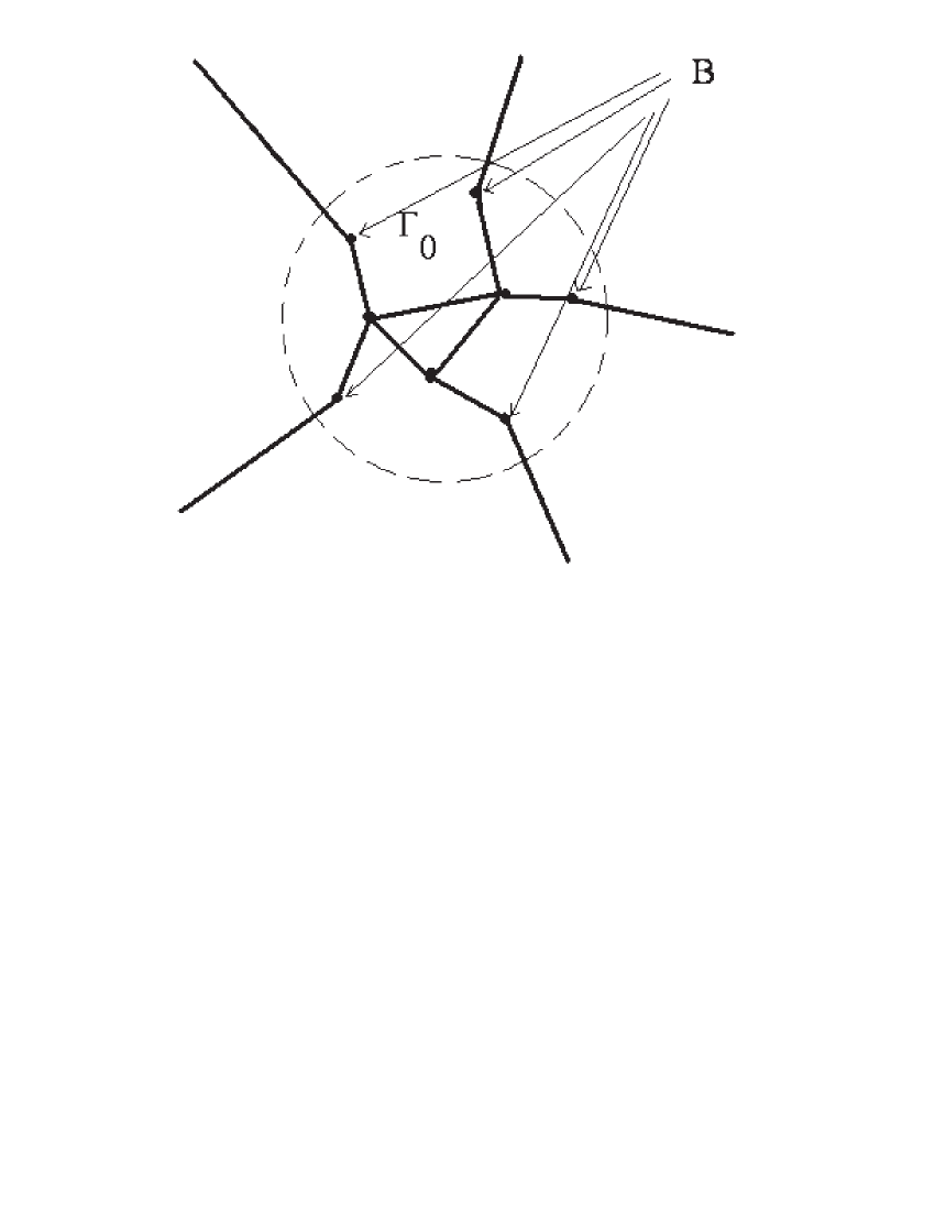
Figure 1. Graph $\Gamma$.

One can naturally define differentiation of functions on $\Gamma$ along the edges, as well as integration over $\Gamma$. In particular, the space $L_{2}(\Gamma)$ can be defined, as well as spaces Sobolev spaces $H^{s}(e)$ of functions on any edge $e$.

This graph is turned into a quantum graph by defining on it a self-adjoint differential operator $H$ as follows:
The operator $H$ acts on functions on $\Gamma$ as the negative second derivative $-\frac{d^{2}}{dx^{2}}$ along the edges. Its domain consists of functions $f$ that belong to the Sobolev space $H^{2}(e)$ on each edge $e$ of $\Gamma$ and satisfy the following boundary conditions at the vertices:

(1) $$A_{v}{\mathbf{f}}(v)+B_{v}{\mathbf{f}^{\prime}}(v)=0\,\,\mbox{for each vertex }v.$$

Here ${\mathbf{f}}(v)$ and ${\mathbf{f}^{\prime}}(v)$ are correspondingly the vector of values of $f$ at $v$ attained from directions of different edges converging at $v$ and the vector of derivatives at $v$ in the outgoing directions. Matrices $A_{v}$ and $B_{v}$ are of size $d_{v}\times d_{v}$, where $d_{v}$ is the degree of $v$ and satisfy the following two conditions:

(2) $$\begin{cases}rank(A_{v}\,\,\,B_{v})=d_{v}\\ A_{v}\times B_{v}^{*}\,\,\mbox{ is self-adjoint}.\\ \end{cases}$$

It is known that (1)-(2) represent the most general (local) self-adjoint boundary value conditions for the operator we consider, see [7, 15] .

We will assume that all “boundary” vertices $v\in B$ have degree two and that the boundary conditions at any such $v$ are “Neumann”:

(3) $$\begin{array}[]{cc}i)&f\mbox{ is continuous at each vertex }v\in B\\ ii)&\mbox{at each vertex }v\in B,\,\sum\limits_{v\in e}\frac{df}{dx_{e}}(v)=0.\\ \end{array}.$$

Here $\sum\limits_{v\in e}\frac{df}{dx_{e}}(v)$ is the sum of the derivatives of $f$ in the outgoing directions along all edges emanating from $v$. In fact, these conditions simply mean that the function and its derivative are both continuous at $v$.

This assumption on the degrees of boundary vertices and on how the conditions look like at the boundary $B$, in fact does not reduce the generality. Indeed, one can always introduce “fake” boundary vertices a little bit further away along the infinite edges and consider them as the new boundary. Then our assumptions are automatically satisfied, and the operator does not change at all.

It is well known (e.g., [7, 15] and references therein), that such defined, the operator $H$ is self-adjoint, bounded below, and in the case of a compact graph (which $\Gamma$ is not, but $\Gamma_{0}$ is) has compact resolvent and thus discrete spectrum. The structure of the spectrum of the operator $H$ on graphs $\Gamma$ of the type described above has been studied for quite a while (e.g., [2, 5, 7, 8, 9, 10, 11, 12, 17, 18, 19, 20, 21]). It is a common knowledge that it possesses continuous part filling the nonnegative half-axis, as well as possibly point spectrum consisting of isolated eigenvalues accumulating to infinity. For completeness, we provide a proof of the following standard statement here (a variation of this proof would use Krein’s resolvent formula) that claims that the continuous part of the spectrum does not depend on a compact part of the graph.

Lemma 1.

In the presence of infinite leads (i.e., if $n>0$), the continuous spectrum of $H$ coincides with the nonnegative half-axis. Eigenvalues of finite multiplicity (including those embedded into the continuous spectrum) accumulating to infinity might be present.

The proof of the lemma uses Glazman’s splitting technique [6]. Let us choose coordinates on each of the infinite leads $e_{v},\,v\in B$ that identify the leads with the nonnegative half axis. We identify the point $v$ with the coordinate $x=0$. So we have $\Gamma=\Gamma_{0}\cup\Gamma_{1}$ where $\Gamma_{1}$ is the disjoint union of $n$ copies of half-axes $[0,\infty)$. Consider the symmetric operator $Q$ that is the restriction of $H$ on the set of those functions $f\in D(H)$ that vanish with their first derivative at all points $v$. Then $Q$ naturally splits into the orthogonal sum of two minimal operators $Q_{0}\bigoplus Q_{1}$ defined on $\Gamma_{0}$ and $\Gamma_{1}$ respectively. Since $Q_{0}$ acts on a compact graph $\Gamma_{0}$ and $Q_{1}$ is just the direct sum of $n$ copies of minimal operators corresponding to $-\frac{d^{2}}{dx^{2}}$ on the half-axis, we conclude that the continuous spectrum of the closure of $Q$ is the same as that of $Q_{1}$. Noticing that $H$ is a finite dimensional extension of $Q$, one can employ Theorems 4 and 11 from [6, Ch. I] to imply the statements of the lemma.

The goal of this paper is to prove a limiting absorption principle and thus absence of the singular continuous spectrum.

Theorem 2.

Let $R(\lambda)$ be the resolvent of $H$ and $f$ be any function from the domain of $H$ that is compactly supported and smooth on each edge. Then the function $(R(\lambda)f,f)$ can be analytically continued from the upper half-plane through $\mathbb{R}^{+}$, except for a discrete subset of $\mathbb{R}^{+}$. In particular, the singular continuous spectrum $\sigma_{sc}(H)$ of $H$ is empty and the absolute continuous spectrum coincides with the nonnegative half axis.

2. Dirichlet-to-Neumann map and other auxiliary considerations

Let us consider the compact part $\Gamma_{0}$ of our graph $\Gamma$ and treat the vertex set $B$ as its “boundary.” We need to define some auxiliary objects related to $\Gamma_{0}$.

First of all, we will consider the operator $H_{0}$ on $L_{2}(\Gamma_{0})$ that acts as the negative second derivative along each edge, and whose domain $D(H_{0})$ consists of those functions from the Sobolev space $H^{2}(e)$ on each edge $e$ of $\Gamma_{0}$ that are equal to zero on $B$ and satisfy conditions (1) at all vertices of $\Gamma_{0}$ except those in $B$. It is standard [15] that this operator is self-adjoint, bounded below, and has compact resolvent, and thus discrete spectrum $\sigma(H_{0})=\{\lambda_{1},...,\lambda_{n},...\}$ accumulating to infinity. We will denote by $R_{0}(\lambda)$ the resolvent of this operator.

One can also define a linear extension operator $E$ acting from functions defined on the (finite) set $B$ into the domain of $H_{0}$

$$E:\mathbb{C}^{n}\mapsto D(H_{0}),$$

such that $(Ef)(v)=f(v)$ for all $v\in B$ and the derivative of $Ef$ at each $v\in B$ along any edge of $\Gamma_{0}$ entering $v$ is equal to zero. Such an operator is indeed easy to construct. For instance, let for any $v\in B$ one defines a function $g_{v}$ such that it is equal to $1$ in a neighborhood of $v$, is smooth on each edge entering $v$, and is supported inside the ball of radius $l_{0}/2$, where $l_{0}$ is the smallest length of an edge of $\Gamma_{0}$. Then one can define $Ef(x)=\sum\limits_{v\in B}f(v)g_{v}(x)$.

Another operator $N$ that we need is an analog of the “normal derivative at the boundary $B$ of $\Gamma_{0}$.” It acts as follows: for any function $f$ on $\Gamma_{0}$ that belongs to $H^{2}(e)$ on any edge $e$, one can define the value $Nf(v)$ for $v\in B$ as the derivative of $f$ at $v$ (taken in the direction towards $v$):

$$Nf(v)=\frac{df}{dx_{e}}(v),$$

where $x_{e}$ is the coordinate along $e$ that increases towards $v$ We remind the reader that each vertex in $B$ has only degree two and only one of the edges connected to each vertex in $B$ belongs to $\Gamma_{0}$. Hence there is no ambiguity in defining $N$ as above.

The main technical tool that we will use is the so called Dirichlet-to-Neumann operator, very popular in inverse problems [20, 23, 24], spectral theory [3, 4], and since recently in quantum graph theory [1, 3, 16] as well. It is a linear operator $\Lambda(\lambda)$ (in our case finite-dimensional) acting on functions defined on $B$, i.e. $\Lambda(\lambda):\mathbb{C}^{n}\mapsto\mathbb{C}^{n}.$ It is defined as follows. Given a function $\phi$ on $B$, one solves the following problem on $\Gamma_{0}$:

(4) $$\begin{cases}-\frac{d^{2}u}{dx^{2}}-\lambda u=0\mbox{ on }\Gamma_{0}\\ \mbox{conditions (\ref{E:vertex_condit}) are satisfied at all vertices of }\Gamma_{0}\mbox{ except those in }B\\ u|_{B}=\phi\\ \end{cases}$$

One now defines the Dirichlet-to-Neumann map as follows:

(5) $$\Lambda(\lambda)\phi=Nu,$$

which justifies the name of the operator. The validity of this definition depends upon (unique) solvability of the problem (4), which holds unless $\lambda\in\sigma(H_{0})$. Thus, $\Lambda(\lambda)$ is defined unless $\lambda\in\sigma(H_{0})$.

Lemma 3.

1. The following operator relation holds:

   (6) $$\Lambda(\lambda)=NR_{0}(\lambda)(\frac{d^{2}}{dx^{2}}+\lambda)E$$

2. The Dirichlet-to-Neumann map $\Lambda(\lambda)$ is a meromorphic matrix valued function of $\lambda$ with poles on the spectrum of $H_{0}$.

3. For real values $\lambda\in\mathbb{R}-\sigma(H_{0})$ the matrix $\Lambda(\lambda)$ is Hermitian.

Proof of the Lemma. Let us introduce a new function $g=u-E\phi$ on $\Gamma_{0}$. By the construction of the extension operator $E$, $g$ clearly satisfies the same vertex conditions (1) on $\Gamma_{0}-B$, as well as the zero Dirichlet conditions on the boundary $g|_{B}=0$. We also note that $Ng=Nu$, since $NE\phi=0$ for any $\phi$. This means that (4) can be equivalently rewritten as

$$\begin{cases}-\frac{d^{2}g}{dx^{2}}-\lambda g=\left(\frac{d^{2}}{dx^{2}}+\lambda\right)E\phi\in L^{2}(\Gamma_{0})\mbox{ on }\Gamma_{0}\\ \mbox{conditions (\ref{E:vertex_condit}) are satisfied at all vertices of }\Gamma_{0}\mbox{ except those in }B\\ g|_{B}=0\\ \end{cases}.$$

In other words, $(H_{0}-\lambda)g=\left(\frac{d^{2}}{dx^{2}}+\lambda\right)E\phi$, which together with the definition of the Dirichlet-to-Neumann map proves the first statement of the Lemma.

The second statement of the lemma immediately follows from the first one together with the discreteness of the spectrum of $H_{0}$ and standard analyticity properties of the resolvent.

The third statement is well known (e.g., [3]) and can be checked by straightforward calculation. ∎

3. Proof of the main result

The proof of Theorem 2 will use the Dirichlet-to-Neumann map to rewrite the spectral problem on $\Gamma$ as a vector valued spectral problem on half-line with a general Robin condition at the origin.

First of all, Lemma 1 implies that it is sufficient to prove absence of singular continuous spectrum on the positive half-axis only. Then the statement about absolute continuous spectrum would follow as well by the same Lemma.

Let $R(\lambda)$ be the resolvent of $H$. The first statement of Theorem 2 is established in the following

Lemma 4.

Let $f$ be a compactly supported function $\Gamma$ which is smooth on each edge and satisfies the vertex conditions (1). Then for any interval $[a,b]\subset\mathbb{R}^{+}$ that does not intersect $\sigma(H_{0})$ one has

(7) $$\mathop{\sup}\limits_{\begin{array}[]{c}a\leq\lambda\leq b\\ 0<\epsilon<1\\ \end{array}}|(R(\lambda+i\epsilon)f,f)|<\infty.$$

In fact, the expression $(R(\lambda)f,f)$ can be analytically continued through such intervals $[a,b]$.

So, now our task is to prove Lemma 4. This will be done using the Dirichlet-to-Neumann operator to reduce the spectral problem for $H$ on $\Gamma$ to a vector one on the half-line.

At this point it will be beneficial to have in mind a different geometric picture of $\Gamma$ than in Fig. 1. Namely, imagine that all the $n$ infinite rays $e_{v},v\in B$ are stretched along the positive half-axis in parallel, being connected at the origin by the finite graph $\Gamma_{0}$ attached to the rays at the vertices of $B$ (see Fig. 2).

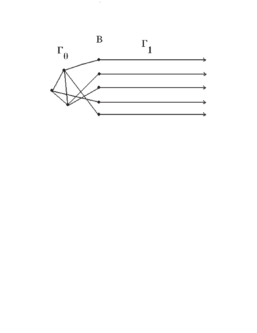
Figure 2. A different visualization of $\Gamma$.

Any function $u$ on $\Gamma$ can now be viewed as the pair $(u_{0},u_{1})$, where $u_{j}=u|_{\Gamma_{j}}$. Functions defined on the part $\Gamma_{1}$ of $\Gamma$ (in particular, $u_{1}$) can be interpreted as vector-valued functions on $\mathbb{R}^{+}$ with values in $\mathbb{C}^{n}$ (recall that $n=|B|$). In particular, interpreting $u_{1}$ as such, we can write $u|_{B}=u_{1}|_{B}=u(0)$, where $0$ is the origin in $\mathbb{R}^{+}$.

Let now $f=(f_{0},f_{1})$ be as in Lemma 4. Then $u=R(\lambda)f$ is a function that belongs to $H^{2}_{loc}$ on each edge and satisfies vertex conditions (1) and the equation

(8) $$Hu-\lambda u=f.$$

Here $u$ naturally depends on $\lambda$. The quantity we need to estimate in (7) is now the inner product $(u,f)=(u_{0},f_{0})+(u_{1},f_{1})$. Let us write (8) and the vertex conditions separately for $u_{0}$ on $\Gamma_{0}$ and $u_{1}$ on $\Gamma_{1}$. On the compact graph $\Gamma_{0}$ we get

(9) $$\begin{cases}(-\frac{d^{2}}{dx^{2}}-\lambda)u_{0}=f_{0}\\ \mbox{(\ref{E:vertex_condit}) satisfied on vertices of }\Gamma_{0}\mbox{ except those in }B\\ u_{0}|_{B}=u_{1}(0)\end{cases}$$

Similarly, on $\Gamma_{1}$ we have

(10) $$\begin{cases}(-\frac{d^{2}}{dx^{2}}-\lambda)u_{1}=f_{1}\mbox{ on }\mathbb{R}^{+}\\ u^{\prime}_{1}(0)=Nu_{0}\end{cases}$$

Here $N$ is the introduced before “normal derivative at $B$” operator on $\Gamma_{0}$ and functions $u_{1},f_{1}$ are interpreted as functions on $\mathbb{R}^{+}$ with values in $\mathbb{C}^{n}$.

Notice that the boundary conditions on $B$ in (9) and at zero in (10) are just the vertex conditions (1) on $B$ rewritten.

If we now are able to express $Nu_{0}$ in terms of $u_{1}(0)$ and $f_{0}$, we will essentially separate problems on $\Gamma_{0}$ and $\Gamma_{1}$. This can easily be done due to Lemma 3. Indeed, if $R_{0}(\lambda)$ is the resolvent of the operator $H_{0}$ studied in the previous section, then clearly one has

(11) $$u_{0}=R_{0}(\lambda)(\frac{d^{2}}{dx^{2}}+\lambda)E(u_{1}(0))+R_{0}(\lambda)f_{0}$$

and thus

(12) $$Nu_{0}=\Lambda(\lambda)u_{1}(0)+NR_{0}(\lambda)f_{0}=\Lambda(\lambda)u_{1}(0)+g(\lambda).$$

Here, for a given $f_{0}$ of the considered class, $g(\lambda)=NR_{0}(\lambda)f_{0}$ is a known meromorphic vector function of $\lambda$ in $\mathbb{C}$ with singularities only at points of $\sigma(H_{0})$.

Now the problem (10) can be rewritten as

(13) $$\begin{cases}(-\frac{d^{2}}{dx^{2}}-\lambda)u_{1}=f_{1}\mbox{ on }\mathbb{R}^{+}\\ u^{\prime}_{1}(0)=\Lambda(\lambda)u_{1}(0)+g(\lambda).\end{cases}$$

By the construction, $\Lambda(\lambda)$ is a meromorphic matrix function in $\mathbb{C}$ with self-adjoint values along the real axis. We also observe that the only memory of the compact part of the graph is confined to the vector-function $g(\lambda)$. We also need to remember that $u_{1}$ must belong to $L^{2}(\mathbb{R}^{+},\mathbb{C}^{n})$.

If we now show that both expressions $(u_{1}(\cdot,\lambda),f_{1}(\cdot))$ and $u_{1}(0,\lambda)$ continue analytically through the real axis except a discrete set, then according to (11) the same will hold for $(u_{0}(\cdot,\lambda),f_{0}(\cdot))$, and thus the Lemma and the main Theorem will be proven. Hence, we only need to concentrate on the vector problem (13) on the positive half-axis.

Let us consider the self-adjoint operator $P$ in $L^{2}(\mathbb{R}^{+})$ naturally corresponding to $-\frac{d^{2}x}{dx^{2}}$ with the Neumann condition at the origin. Let also $r(\lambda)$ be its resolvent. We sketch below the proof of the following well known limiting absorption result:

Lemma 5.

For any smooth compactly supported function $f$ on $\mathbb{R}^{+}$ and any interval $(a,b)\subset\mathbb{R}^{+}$, the inner product $(r(\lambda)f,f)$ as a function of $\lambda$ can be analytically continued through $(a,b)$ from the upper half-plane $\mbox{Im}\;\;\lambda>0$.

Let us chose in the upper half-plane the branch of $\sqrt{\lambda}$ that has positive imaginary part. The above lemma then follows immediately from the explicit formula for $r(\lambda)$:

(14) $$(r(\lambda)f)(x)=\frac{i}{2}\int_{0}^{\infty}\frac{e^{i\sqrt{\lambda}(x+s)}+e^{i\sqrt{\lambda}|x-s|}}{\sqrt{\lambda}}f(s)\;ds.$$

This formula also implies that the value $(r(\lambda)f)(0)$ has the same analyticity property.

In what follows we will abuse notations using $r(\lambda)$ where in fact one should use $r(\lambda)\bigotimes I$ (here $I$ is the unit $n\times n$ matrix).

It is not hard to solve (10) now. Indeed, after a simple computation one arrives to the formula for the solution that one can check directly when $\mbox{Im}\;\;\sqrt{\lambda}>0$:

(15) $$u_{1}(x,\lambda):=(r(\lambda)f_{1})(x)-ie^{i\sqrt{\lambda}x}A(\lambda)$$

where the vector $A(\lambda)$ is:

(16) $$A(\lambda)=\Lambda(\lambda)[\sqrt{\lambda}+i\Lambda(\lambda)]^{-1}(r(\lambda)f_{1})(0)+\frac{g(\lambda)}{\sqrt{\lambda}}$$

Notice that the matrix function $\sqrt{\lambda}+i\Lambda(\lambda)$ is meromorphic on the Riemann surface of $\sqrt{\lambda}$. Due to self-adjointness of $\Lambda(\lambda)$, the values of that function for non-zero real $\lambda$ are invertible. Hence, the matrix function $\left(\sqrt{\lambda}+i\Lambda(\lambda)\right)^{-1}$ is meromorphic on the same Riemann surface.

Now the quantity of interest becomes

(17) $$(u_{1}(\cdot,\lambda),f_{1}(\cdot))=(r(\lambda)f_{1},f_{1})-i(e^{i\sqrt{\lambda}x}A(\lambda),f_{1}(x)).$$

Lemma 5 implies the needed analyticity of the first term in the sum. Since $\mbox{Im}\,\sqrt{\lambda}>0$, according to the remarks after (14), $(r(\lambda)f_{1})(0)$ is analytic hence $e^{i\sqrt{\lambda}x}A(\lambda)$ is analytic through $(a,b)$ as well save for a discrete set of $\lambda$. Thus the final term in the sum can also be analytically continued through $(a,b)$ as well outside of a discrete set of $\lambda$.

This finishes the proof of Lemma 4.∎

Since the space of functions $f$ as above is dense in $L^{2}(\Gamma)$, it is well known that (7) implies absence of the singular continuous spectrum (e.g., [25, Proposition 2 and (18) in Section 1.4.5], [22, pp. 136-139 in Section XIII.6] and thus proves Theorem 2.

4. Remarks and acknowledgments

A procedure similar to the one we use to switch from general Robin type condition condition to a Neumann condition in (13) was employed in [1].

The author would like to thank Prof. Peter Kuchment for his help and suggestions.

This work was partially supported by the NSF Grants DMS 0296150, 0072248, and 0406022. The author expresses his gratitude to NSF for this support. The content of this paper does not necessarily reflect the position or the policy of the NSF and the federal government, and no official endorsement should be inferred.

References

- [1] J. D. Bondurant and S. A. Fulling, The Dirichlet-to-Robin transform, J. Phys. A 38 (2005), 1505–1532.
- [2] P. Exner, P. Šeba, Free quantum motion on a branching graph, Rep. Math. Phys. 28 (1989), 7-26.
- [3] C. Fox, V. Oleinik, and B. Pavlov, Dirichlet-to-Neumann map machinery for resonance gaps and bands of periodic networks, preprint 2004.
- [4] L. Friedlander, On the spectrum of a class of second order periodic elliptic differential operators, Comm. Partial Diff. Equat. 15(1990), 1631–1647.
- [5] N. Gerasimenko and B. Pavlov, Scattering problems on non-compact graphs, Theor. Math. Phys., 74 (1988), no.3, 230–240.
- [6] I. M. Glazman, Direct Methods of Qualitative Spectral Analysis of Singular Differential Operators, Isr. Progr. Sci. Transl., Jerusalem 1965.
- [7] V. Kostrykin and R. Schrader, Kirchhoff’s rule for quantum wires, J. Phys. A 32(1999), 595-630.
- [8] V. Kostrykin and R. Schrader, Kirchhoff’s rule for quantum wires. II: The inverse problem with possible applications to quantum computers, Fortschr. Phys. 48(2000), 703–716.
- [9] V. Kostrykin and R. Schrader, The generalized star product and the factorization of scattering matrices on graphs, J. Math. Phys. 42(2001), 1563–1598.
- [10] T. Kottos and U. Smilansky, Quantum chaos on graphs, Phys. Rev. Lett. 79(1997), 4794–4797.
- [11] T. Kottos and U. Smilansky, Periodic orbit theory and spectral statistics for quantum graphs, Ann. Phys. 274 (1999), 76–124.
- [12] T. Kottos and U. Smilansky, Chaotic scattering on graphs, Phys. Rev. Lett. 85(2000), 968–971.
- [13] P. Kuchment, Differential and pseudo-differential operators on graphs as models of mesoscopic systems, in Analysis and Applications, H. Begehr, R. Gilbert, and M. W. Wang (Editors), Kluwer Acad. Publ. 2003, 7-30.
- [14] P. Kuchment, Graph models of wave propagation in thin structures, Waves in Random Media 12(2002), no. 4, R1-R24.
- [15] P. Kuchment, Quantum graphs I. Some basic structures, Waves in Random media, 14 (2004), S107–S128.
- [16] P. Kuchment, Quantum graphs II, J. Phys. A: Math. Gen. 38 (2005),4887–4900.
- [17] Yu. B. Melnikov and B. S. Pavlov, Two-body scattering on a graph and application to simple nanoelectronic devices, J. Math. Phys. 36(1995), 2813-2825.
- [18] A. Mikhailova, B. Pavlov, and L. Prokhorov, Modelling quantum networks, arXiv:math-ph/0312038.
- [19] B. S. Pavlov and M. D. Faddeev, A model of free electrons and the scattering problem, Theor. and Math. Phys. 55(1983), no.2, 485–492
- [20] B. Pavlov, -matrix and Dirichlet-to-Neumann operators, in Scattering (Encyclopedia of scattering), R. Pike and P. Sabatier (Eds.), Acad. Press. 2001, pp. 1678–1688.
- [21] Quantum Graphs and Their Applications, P. Kuchment (Editor), special issue of Waves in Random Media 14 (2004), no. 1.
- [22] M. Reed and B. Simon, Methods of Modern Mathematical Physics v. 4, Acad. Press, NY 1978.
- [23] J. Sylvester and G. Uhlmann, The Dirichlet to Neumann map and its applications, in Inverse Problems in Partial Differential Equations, SIAM, 1990, pp. 101–139.
- [24] G. Uhlmann, Inverse boundary value problems and applications, Asterisque 207(1992), 153–211.
- [25] D. Yafaev, Mathematical Scattering Theory, AMS, Providence, RI 1992.