Geometric tri-product of the spin domain and Clifford algebras

Abstract

We show that the triple product defined by the spin domain (Bounded Symmetric Domain of type 4 in Cartan’s classification) is closely related to the geometric product in Clifford algebras. We present the properties of this tri-product and compare it with the geometric product.

The spin domain can be used to construct a model in which spin 1 and spin1/2 particles coexist. Using the geometric tri-product, we develop the geometry of this domain. We present a geometric spectral theorem for this domain and obtain both spin 1 and spin 1/2 representations of the Lorentz group on this domain.

MSC: 15A66; 17C90

PACS: 02.10.De; 12.60.Jv.

Keywords: Spin triple product; Spin domain; Geometric product; Lorentz group representations.

1 Introduction

The spin factor, a bounded symmetric domain of type IV in the Cartan classification [3], plays an important role in physics. It was shown in [7] that the state space of any two-state quantum system is the dual of a complex spin factor. In [4] and [9] it was shown that a new dynamic variable, called $s$ velocity, which is a relativistic half of the usual velocity, is useful for solving explicitly relativistic dynamic equations. In [4] it was shown that automorphism group of this $s$ velocity coincide with the conformal group and its Lie algebra is described by the triple product defined uniquely by the spin domain. The basic operators of the complex spin triple product are closely related to the geometric product of Clifford algebras.

We start by defining the spin triple product, which we also call the geometric tri-product, and discuss its connection to the geometric product in Clifford algebras. Then we study the algebraic properties and the geometry of the unit ball of the spin factor and its dual. Here, the duality between minimal and maximal tripotents plays a central role. In particular, this duality enables us to construct both spin 1 and spin 1/2 representations of the Lorentz group on the same spin factor. Thus, we can incorporate particles of integer and half-integer spin in one model. As a result, the complex spin factor with its triple product is a new model for supersymmetry.

Most of the results of this article appear in full detail in Chapter 3 of [4].

2 The geometric tri-product of the spin domain

Let $\mathbf{C}^{n}$ denote $n$-dimensional (finite or infinite) complex Euclidean space with the natural basis

$$\mathbf{e}_{1}=(1,0,\ldots,0),\mathbf{e}_{2}=(0,1,\ldots,0),\dots,\mathbf{e}_{n}=(0,\ldots,0,1)$$

and the usual inner product

$$\langle\mathbf{a}|\mathbf{b}\rangle=a_{1}\overline{b}_{1}+a_{2}\overline{b}_{2}+\cdots+a_{n}\overline{b}_{n},$$ (1)

where $\mathbf{a}=(a_{1},\ldots,a_{n}),\;\mathbf{b}=(b_{1},\ldots,b_{n})$. The Euclidean norm of $\mathbf{a}$ is defined by $|\mathbf{a}|=\langle\mathbf{a}|\mathbf{a}\rangle^{1/2}$. As in [8], [4], we define a triple product on $\mathbf{C}^{n}$ by

$$\{\mathbf{a},\mathbf{b},\mathbf{c}\}=\langle\mathbf{a}|\mathbf{b}\rangle\mathbf{c}+\langle\mathbf{c}|\mathbf{b}\rangle\mathbf{a}-\langle\mathbf{a}|\mathbf{\overline{c}}\rangle\overline{\mathbf{b}},$$ (2)

where $\overline{\mathbf{b}}=(\overline{b}_{1},\ldots,\overline{b}_{n})$ denotes the complex conjugate of $\mathbf{b}$. In [4] this product is called the spin triple product. In this paper we will also call it also the geometric tri-product.

Note that the geometric tri-product is linear in the first and third variables ($\mathbf{a}$ and $\mathbf{c}$) and conjugate linear in the second variable ($\mathbf{b}$). Since, by the definition of the inner product, we have $\langle\mathbf{a}|\mathbf{\overline{c}}\rangle=\langle\mathbf{c}|\mathbf{\overline{a}}\rangle$, the triple product is symmetric in the outer variables, i.e.,

$$\{\mathbf{a},\mathbf{b},\mathbf{c}\}=\{\mathbf{c},\mathbf{b},\mathbf{a}\}.$$ (3)

The space ${C}^{n}$ with the geometric tri-product is called the complex spin triple factor and will be denoted by $\mathcal{S}^{n}$. We use this name because if we define a norm based on this triple product, then the unit ball of $\mathcal{S}^{n}$ is a domain of Cartan type IV known as the spin factor.

The real part of the spin factor, denoted $\mathcal{S}^{n}_{\mathbf{R}}$, is the subspace of $\mathcal{S}^{n}$ defined by

$$\mathcal{S}^{n}_{\mathbf{R}}=\{\mathbf{a}\in\mathcal{S}^{n}:\;\;\;\overline{\mathbf{a}}={\mathbf{a}}\},$$

or, equivalently,

$$\mathcal{S}^{n}_{\mathbf{R}}=\mbox{span}_{\mathbf{R}}\{\mathbf{e}_{j}\}.$$ (4)

This subspace is identical, as a linear space, to $R^{n}$ and its tri-product defines the Lie algebra of the conformal group of the unit disk in $R^{n}$.

For any $\mathbf{a},\mathbf{b}\in\mathcal{S}^{n}$, we define a complex linear map $D(\mathbf{a},\mathbf{b}):\mathcal{S}^{n}\rightarrow\mathcal{S}^{n}$ by

$$D(\mathbf{a},\mathbf{b})\mathbf{z}=\{\mathbf{a},\mathbf{b},\mathbf{z}\}=\langle\mathbf{a}|\mathbf{b}\rangle\mathbf{z}+\langle\mathbf{z}|\mathbf{b}\rangle\mathbf{a}-\langle\mathbf{a}|\mathbf{\overline{z}}\rangle\overline{\mathbf{b}}.$$ (5)

The linear map defined by $D(\mathbf{a},\mathbf{b})$ can be expressed in the language of Clifford algebras by

$$D(\mathbf{a},\mathbf{b})=\langle\mathbf{a}|\mathbf{b}\rangle\,I+\mathbf{a}\wedge\mathbf{b},$$ (6)

where $I$ denotes the identity operator and

$$(\mathbf{a}\wedge\mathbf{b})(\mathbf{z})=\langle\mathbf{z}|\mathbf{b}\rangle\mathbf{a}-\langle\mathbf{a}|\mathbf{\overline{z}}\rangle\overline{\mathbf{b}}.$$

By a commonly used identity [10], in the real case $\mathbf{a}\wedge\mathbf{b}$ coincides with the wedge (exterior) product of vectors:

$$\mathbf{z}\cdot(\mathbf{a}\wedge\mathbf{b})=(\mathbf{z}\cdot\mathbf{a})\mathbf{b}-(\mathbf{z}\cdot\mathbf{b})\mathbf{a}.$$

Thus, the map $D(\mathbf{a},\mathbf{b})$ resembles the geometric product of $\mathbf{a}$ and $\mathbf{b}$, defined by

$$\mathbf{a}\mathbf{b}=\langle\mathbf{a}|\mathbf{b}\rangle+\mathbf{a}\wedge\mathbf{b},$$ (7)

where the sum of a scalar $\langle\mathbf{a}|\mathbf{b}\rangle$ and the antisymmetric bivector $\mathbf{a}\wedge\mathbf{b}$ belongs to the Clifford algebra. Hence, the operator $D(\mathbf{a},\mathbf{b})$ is a natural operator on the spin factor and plays a role similar to that of the geometric product.

3 The canonical basis of $\mathcal{S}^{n}$.

The canonical anticommutation relations (CAR) are the basic relations used in the description of fermion fields.

We will show now that the natural basis of $\mathcal{S}^{n}$ satisfies a triple analog of the CAR. Recall that the classical definition of CAR involves a sequence $p_{k}$ of elements of an associative algebra which satisfy the relations

$$p_{l}p_{k}+p_{k}p_{l}=2\delta_{kl},$$ (8)

where $\delta_{kl}$ denotes the Kronecker delta. This implies that $p_{k}^{2}=1,$ and, therefore,

$$p_{k}p_{k}p_{l}=p_{l},\quad\mbox{ for any }1\leq k,l\leq n.$$ (9)

Multiplying (8) on the left by $p_{l}$, we get

$$p_{l}p_{k}p_{l}=-p_{k},\quad\mbox{ for }k\neq l.$$ (10)

We call the relations (9) and (10) the triple canonical anticommutation relations (TCAR).

Using definition (2) of the spin triple product, it is easy to verify that the elements $\mathbf{e}_{1},\mathbf{e}_{2},\ldots,\mathbf{e}_{n}$ of the natural basis of the spin triple factor satisfy the following relations:

$$\{\mathbf{e}_{l},\mathbf{e}_{k},\mathbf{e}_{l}\}=-\mathbf{e}_{k},\;\;\;\mbox{ for }k\neq l,$$ (11)

$$\{\mathbf{e}_{l},\mathbf{e}_{k},\mathbf{e}_{k}\}=\{\mathbf{e}_{k},\mathbf{e}_{k},\mathbf{e}_{l}\}=\mathbf{e}_{l},\;\;\mbox{ for any}\;\;k,l,$$ (12)

$$\{\mathbf{e}_{l},\mathbf{e}_{k},\mathbf{e}_{m}\}=0,\quad\mbox{for }\;k,l,m\;\mbox{distinct}.$$ (13)

Thus, the natural basis of the spin triple factor $\mathcal{S}^{n}$ or $\mathcal{S}^{n}_{\mathbf{R}}$ satisfies the TCAR. Conversely, if we define a ternary operation on $\{\mathbf{e}_{l},\mathbf{e}_{2},\ldots,\mathbf{e}_{n}\}$ which satisfies (11)-(13), then the resulting triple product on $\mathcal{S}^{n}$ will be exactly the spin triple product.

We say that a basis $\{\mathbf{u}_{1},\mathbf{u}_{2}\ldots,\mathbf{u}_{n}\}$ of $\mathcal{S}^{n}$ is a canonical basis of $\mathcal{S}^{n}$ or a TCAR basis if it satisfies (11)-(13). It can be shown that any TCAR basis is an orthonormal basis of $\mathbf{C}^{n}$. The converse, however, is not true.

Let $\mathbf{u}_{l},\mathbf{u}_{k}$ be any two distinct elements of an orthonormal basis in $R^{n}$ spanning a plane $\Pi=\mbox{span}_{R}\{\mathbf{u}_{l},\mathbf{u}_{k}\}$ in $R^{n}$. Then, the generator of rotations in $\Pi$ is defined by

$$J(\mathbf{u}_{l})=-\mathbf{u}_{k},\;\;J(\mathbf{u}_{k})=\mathbf{u}_{l},\mbox{ and }J(\mathbf{u}_{m})=0,\quad\mbox{for }\;k,l,m\;\mbox{distinct}.$$ (14)

From (11)-(13), it follows that the operator $D(\mathbf{u}_{l},\mathbf{u}_{k})$ is the generator of rotation in the plane $\Pi=\mbox{span}_{R}\{\mathbf{u}_{l},\mathbf{u}_{k}\}$ of $\mathcal{S}^{n}$, implying that

$$\exp(\theta D(\mathbf{u}_{l},\mathbf{u}_{k}))\;\mbox{ = rotation in $\Pi$ of $\mathcal{S}^{n}$ by the angle }-\theta.$$ (15)

Note that properties (11)-(13) can be derived from the requirement that the operator $D(\mathbf{u}_{l},\mathbf{u}_{k})$ is the generator of rotation in the plane $\Pi=\mbox{span}_{R}\{\mathbf{u}_{l},\mathbf{u}_{k}\}$ of $\mathcal{S}^{n}$. This result is similar to the fact [2] that bivectors play the role of generators of rotations.

On the other hand, since $D(\mathbf{u}_{k},i\mathbf{u}_{k})=-iD(\mathbf{u}_{k},\mathbf{u}_{k})=-i\,I$, we have

$$\exp(\theta D(\mathbf{u}_{k},i\mathbf{u}_{k}))\mathbf{a}=e^{-i\theta}\mathbf{a}$$ (16)

for any $\mathbf{a}\in\mathcal{S}^{n}$. This shows that $D(\mathbf{u}_{k},i\mathbf{u}_{k})$ is the generator of the rotation representing the action of $U(1)$ on $\mathcal{S}^{n}$.

To define reflection in a plane, we will use the tri-product operator $Q(\mathbf{u})$ defined by

$$Q(\mathbf{u})\mathbf{a}=\{\mathbf{u},\mathbf{a},\mathbf{u}\}$$ (17)

for $\mathbf{a}\in\mathcal{S}^{n}$. Direct calculation using the definition (2) of the geometric tri-product shows that if $|\mathbf{u}|=1,$ then

$$Q(\mathbf{u})\mathbf{a}=\{\mathbf{u},\mathbf{a},\mathbf{u}\}=2\langle\mathbf{u}|\mathbf{a}\rangle\mathbf{u}-\mathbf{a}=2P_{\mathbf{u}}\mathbf{a}-\mathbf{a},$$ (18)

where $P_{\mathbf{u}}\mathbf{a}$ denotes the orthogonal projection of $\mathbf{a}$ onto the direction of $\mathbf{u}$. Note that for the 3D-space $\mathcal{S}_{\mathbf{R}}^{3}$ the operator $-Q(\mathbf{u})$ defines the space reflection with respect to the plane with normal $\mathbf{u}$. In $\mathcal{S}^{n}$, $180^{\circ}$ rotation in the plane $\Pi=\mbox{span}_{R}\{\mathbf{u}_{k},\mathbf{u}_{l}\}$ is given by

$$Q(\mathbf{u}_{l})Q(\mathbf{u}_{k}):\;\mathbf{a}\;\rightarrow\;\{\mathbf{u}_{l},\{\mathbf{u}_{k},\mathbf{a},\mathbf{u}_{k}\},\mathbf{u}_{l}\}.$$ (19)

Moreover, rotation operator in the above plane $\Pi$ by an angle $\theta$ can be obtained as a double reflection in two planes with an angle $\theta/2$ between their normals, as

$$Q(\exp(\frac{\theta}{2}D(\mathbf{u}_{l},\mathbf{u}_{k})\mathbf{u}_{k})Q(\mathbf{u}_{k}).$$ (20)

The natural morphisms of the complex spin triple factor $\mathcal{S}^{n}$ are the linear, invertible maps (bijections) $T:\mathcal{S}^{n}\rightarrow\mathcal{S}^{n}$ which preserve the triple product. This means that

$$T\{\mathbf{a},\mathbf{b},\mathbf{c}\}=\{T\mathbf{a},T\mathbf{b},T\mathbf{c}\}.$$ (21)

Such a linear map is called a triple automorphism of $\mathcal{S}^{n}$. We denote by $\mbox{Taut}\,(\mathcal{S}^{n})$ the group of all triple automorphisms of $\mathcal{S}^{n}$.

Since the definition of a TCAR basis involves only the triple product, it is obvious that a triple automorphism $T$ maps a TCAR basis into a TCAR basis. In particular, the image of the natural basis $\{\mathbf{e}_{1},\mathbf{e}_{2},\ldots,\mathbf{e}_{n}\}$ is a TCAR basis. It can be shown that a bijective map $T$ of the spin triple factor $\mathcal{S}^{n}$ preserves the triple product, i.e. $T\in\mbox{Taut}\,(\mathcal{S}^{n})$, if and only if it has the form $T=\lambda U$, where $\lambda$ is a complex number of absolute value 1 and $U$ is orthogonal. Thus,

$$\mbox{Taut}\,(\mathcal{S}^{n})=U(1)\times O(n),$$ (22)

where $U(1)$ is the group of rotations in the complex plane and $O(n)$ is the orthogonal group of dimension $n$. Thus, ${Taut}\,(\mathcal{S}^{n})$ is a Lie group with real dimension $\frac{n(n-1)}{2}+1$.

This group is a natural candidate for the description of the state space of a quantum system. The state description of a quantum system is often given by a complex-valued wave function $\psi(\mathbf{r})$, where $\mathbf{r}\in R^{3}$. This description is invariant under the choice of the orthogonal basis in $R^{3}$, implying that there is a natural action of the group $O(3)$ on the state space. In the presence of an electromagnetic field, the gauge of the field induces a multiple of the state by a complex number $\lambda,\;|\lambda|=1$, which will not affect any meaningful results. Multiplication of all $\psi(\mathbf{r})$ by such a $\lambda$ corresponds to an action of the group $U(1)$ on this state space. Moreover, even without gauge invariance, all meaningful quantities in quantum mechanics are invariant under multiplication by a complex number of absolute value $1$, resulting in an action of $U(1)$. Thus, $\mbox{Taut}\,(\mathcal{S}^{n})$ acts naturally on the state space of quantum systems. A similar result holds for quantum fields.

4 Tripotents and singular decomposition in $\mathcal{S}^{n}$

The building blocks of binary operations, are the projections. These are the idempotents of the operation, that is, non-zero elements $p$ that satisfy $p^{2}=p.$ For a ternary operation, the building blocks are the tripotents, non-zero elements $\mathbf{u}$ satisfying $\{\mathbf{u},\mathbf{u},\mathbf{u}\}=\mathbf{u}.$ To describe the tripotents $\mathbf{u}\in\mathcal{S}^{n},$ we introduce the notion of determinant for elements of $\mathcal{S}^{n}.$ For any $\mathbf{a}\in\mathcal{S}^{n}$, the determinant of $\mathbf{a}$, denoted $\det\mathbf{a}$, is

$$\det\mathbf{a}=\langle\mathbf{a}|\overline{\mathbf{a}}\rangle=\sum_{i=1}^{n}a_{i}^{2}.$$ (23)

In case the elements of $\mathcal{S}^{n}$ can be represented by matrices, this definition agrees with the ordinary determinant of a matrix. This definition is similar to the notion of metric on a paravector space (see [2]). Note that elements with zero determinant are called null-vectors in the literature.

The properties of the tripotents $\mathbf{u}\in\mathcal{S}^{n}$ are summarized in Table 1:

Table 1: The algebraic properties of tripotents in $\mathcal{S}^{n}.$

There are only two types of tripotents in $\mathcal{S}^{n}$,maximal and minimal. The Euclidian norm of a maximal tripotent is 1, while the norm of a minimal tripotent is $1/\sqrt{2}$. For a maximal tripotent $\mathbf{u}$, we have $|\det\mathbf{u}|=1$, while for a minimal tripotent $\mathbf{v}$, we have $\det\mathbf{v}=0.$ The operator $D(\mathbf{u},\mathbf{u})$ for a maximal tripotent $\mathbf{u}$ is the identity operator. For a minimal tripotent $\mathbf{v}$, the operator $D(\mathbf{v},\mathbf{v})$ is

$$D(\mathbf{v},\mathbf{v})=\frac{1}{2}(I+P_{\mathbf{v}}-P_{\overline{\mathbf{v}}}),$$ (24)

where $P_{\mathbf{v}}$ and $P_{\overline{\mathbf{v}}}$ denote the orthogonal projections on ${\mathbf{v}}$ and $\overline{\mathbf{v}}$ respectively.

If we decompose a minimal tripotent $\mathbf{v}$ into real and imaginary parts as

$$\mathbf{v}=\mathbf{x}+i\mathbf{y},\quad\;\;\mathbf{x},\mathbf{y}\in\mathcal{S}^{n}_{\mathbf{R}},$$ (25)

then, $\langle\mathbf{x}|\mathbf{y}\rangle=0$ and $|\mathbf{x}|=|\mathbf{y}|=1/2$. Similarly, if we decompose a maximal tripotent $\mathbf{u}$ into real and imaginary parts, then there exist a real $\theta$ and $\mathbf{r}\in\mathcal{S}_{\mathbf{R}}^{n}$ with $|\mathbf{r}|=1$ such that

$$\mathbf{u}=\cos\theta\,\mathbf{r}+i\sin\theta\,\mathbf{r}=e^{i\theta}\mathbf{r}.$$ (26)

The spectrum of the operator $D(\mathbf{v},\mathbf{v})$ is the set $\{1,1/2,0\}$, where the eigenvalue 1 is obtained on multiples of $\mathbf{v}$ (i.e., on the image of $P_{\mathbf{v}}$), the eigenvalue 0 is obtained on multiples of $\overline{\mathbf{v}}$ (on the image of $P_{\overline{\mathbf{v}}}$) and the eigenvalue $1/2$ is obtained on the image of the projection $I-P_{\mathbf{v}}-P_{\overline{\mathbf{v}}}.$ Let $P_{1}(\mathbf{v})$, $P_{1/2}(\mathbf{v})$ and $P_{0}(\mathbf{v})$ be the projections onto the $1$, $1/2$ and $0$ eigenspaces of $D(\mathbf{v},\mathbf{v})$, respectively:

$$P_{1}(\mathbf{v})=P_{\mathbf{v}},\;\;P_{1/2}(\mathbf{v})=I-P_{\mathbf{v}}-P_{\overline{\mathbf{v}}},\;\;P_{0}(\mathbf{v})=P_{\overline{\mathbf{v}}}.$$ (27)

Then

$$D(\mathbf{v})=P_{1}(\mathbf{v})+\frac{1}{2}P_{1/2}(\mathbf{v}).$$ (28)

Since

$$I=P_{1}(\mathbf{v})+P_{1/2}(\mathbf{v})+P_{0}(\mathbf{v}),$$ (29)

these projections induce a decomposition of $\mathcal{S}^{n}$ into the sum of the three eigenspaces:

$$\mathcal{S}^{n}=\mathcal{S}^{n}_{1}(\mathbf{v})+\mathcal{S}^{n}_{1/2}(\mathbf{v})+\mathcal{S}^{n}_{0}(\mathbf{v}).$$ (30)

This is called the Peirce decomposition of $\mathcal{S}^{n}$ with respect to a minimal tripotent $\mathbf{v}.$ A very useful result for calculations is the Peirce calculus formula. Let $j,k,l\in\{1,\frac{1}{2},0\}$ with $j-k+l\in\{1,\frac{1}{2},0\}$, then

$$\{\mathcal{S}^{n}_{j}(\mathbf{v}),\mathcal{S}^{n}_{k}(\mathbf{v}),\mathcal{S}^{n}_{l}(\mathbf{v})\}\subset\mathcal{S}^{n}_{j-k+l}(\mathbf{v}).$$ (31)

Otherwise, $\{\mathcal{S}^{n}_{j}(\mathbf{v}),\mathcal{S}^{n}_{k}(\mathbf{v}),\mathcal{S}^{n}_{l}(\mathbf{v})\}=0.$

We will say that two tripotents $\mathbf{v}$ and $\mathbf{u}$ are algebraically orthogonal (denoted by $\mathbf{v}\perp\mathbf{u}$) if

$$D(\mathbf{v},\mathbf{v})\mathbf{u}=0,\mbox{ or }D(\mathbf{u},\mathbf{u})\mathbf{v}=0.$$ (32)

It can be shown that $\mathbf{v}$ and $\mathbf{u}$ are algebraically orthogonal if and only if

$$\mathbf{v}\perp\mathbf{u}\quad\Leftrightarrow\quad D(\mathbf{v},\mathbf{u})=0.$$ (33)

Such tripotents are the analog of nonzero zero-divisors in an algebra. For a minimal tripotent $\mathbf{v}$, its complex adjoint $\overline{\mathbf{v}}$ is also a minimal tripotent and is algebraically orthogonal to $\mathbf{v}$. Moreover, and $\mathbf{v}+\overline{\mathbf{v}}$ is a maximal tripotent. Thus, for a minimal tripotent $\mathbf{v}$

$$D(\mathbf{v},\overline{\mathbf{v}})=0,\;\;\mbox{ and }\;\;D(\mathbf{v}+\overline{\mathbf{v}},\mathbf{v}+\overline{\mathbf{v}})=I.$$ (34)

Let $\mathbf{a}$ be any element in $\mathcal{S}^{n}.$ If $\det\mathbf{a}=0$, then $\mathbf{a}$ is a positive multiple of a minimal tripotent. In fact, $\mathbf{u}:=\frac{1}{\sqrt{2}}\frac{\mathbf{a}}{|\mathbf{a}|}$ is a minimal tripotent. If $\det\mathbf{a}\neq 0$, it can be shown that there exist an algebraically orthogonal pair $\mathbf{v}_{1},\mathbf{v}_{2}$ of minimal tripotents and a pair of non-negative real numbers $s_{1},s_{2}$, called the singular numbers of $\mathbf{a}$, such that $s_{1}\geq s_{2}\geq 0$ and

$$\mathbf{a}=s_{1}\mathbf{v}_{1}+s_{2}\mathbf{v}_{2}.$$ (35)

This decomposition is called the singular decomposition of $\mathbf{a}.$ If $\mathbf{a}$ is not a multiple of a maximal tripotent, then $s_{1}>s_{2}$ and the decomposition is unique. If $\mathbf{a}$ is a multiple of a maximal tripotent, then $s_{1}=s_{2}$, and the decomposition is, in general, not unique.

The singular numbers satisfy

$$|\mbox{det}\,\mathbf{a}|=s_{1}s_{2},$$ (36)

which corresponds to the fact that the determinant of a positive operator is the product of its eigenvalues, and

$$s_{1}\pm s_{2}=\sqrt{2|\mathbf{a}|^{2}\pm 2|\mbox{det}\,\mathbf{a}|}.$$ (37)

Given $\mathbf{a}$ with singular decomposition (35), we have

$$\mathbf{a}^{(3)}:=\{\mathbf{a},\mathbf{a},\mathbf{a}\}=s_{1}^{3}\mathbf{v}_{1}+s_{2}^{3}\mathbf{v}_{2},$$ (38)

showing that the cube of an element $\mathbf{a}\in\mathcal{S}^{n}$ can be calculated by cubing its singular numbers. Similarly, taking any odd power of $\mathbf{a}$ is equivalent to applying this odd power to its singular numbers. Moreover, for any analytic function $f:R_{+}\to R_{+}$ we can define

$$f(\mathbf{a})=f(s_{1})\mathbf{v}_{1}+f(s_{2})\mathbf{v}_{2},$$ (39)

which play the analog of operator function calculus.

For an arbitrary element $\mathbf{d}\in\mathcal{S}^{n}$, it can be shown that the spectrum of the linear operator $D(\mathbf{d},\mathbf{d})$ is non-negative and that

$$D(\mathbf{d},\mathbf{d})\{\mathbf{a},\mathbf{b},\mathbf{c}\}=\{D(\mathbf{d},\mathbf{d})\mathbf{a},\mathbf{b},\mathbf{c}\}-\{\mathbf{a},D(\mathbf{d},\mathbf{d})\mathbf{b},\mathbf{c}\}+\{\mathbf{a},\mathbf{b},D(\mathbf{d},\mathbf{d})\mathbf{c}\}.$$ (40)

This is called the main identity of the triple product. Note that from this identity follows that $D(\mathbf{d},\mathbf{d})$ is a triple derivation and thus its exponent is a triple automorphism.

5 Geometry of the unit ball of the spin factor

Let $\mathbf{a}\in\mathcal{S}^{n}$ have singular decomposition (35). We define a new norm, called the operator norm of a, by

$$\|\mathbf{a}\|=s_{1}.$$ (41)

This norm satisfies the triple analog of the “star identity,” namely $\|\{\mathbf{a},\mathbf{a},\mathbf{a}\}\|=\|\mathbf{a}\|^{3}$. Moreover,

$$\|\mathbf{a}\|=\frac{1}{\sqrt{2}}(\sqrt{|\mathbf{a}|^{2}+|\det\mathbf{a}|}+\sqrt{|\mathbf{a}|^{2}-|\det\mathbf{a}|}).$$ (42)

The operator norm can also be defined by

$$\|\mathbf{a}\|^{2}=\|D(\mathbf{a},\mathbf{a})\|_{op},$$ (43)

where $\|D(\mathbf{a},\mathbf{a})\|_{op}$ denotes the operator norm of $D(\mathbf{a},\mathbf{a}).$ Since

$$|\mathbf{a}|\leq\|\mathbf{a}\|\leq\sqrt{2}|\mathbf{a}|,$$ (44)

the operator norm is equivalent to the Euclidean norm on $\mathbf{C}^{n}.$

We denote the unit ball of $\mathcal{S}^{n}$ by

$$D_{s,n}=\{\mathbf{a}\in\mathcal{S}^{n}:\;\;\|\mathbf{a}\|\leq 1\}.$$ (45)

The intersection of this ball with $\mathcal{S}^{n}_{\mathbf{R}}$ is the Euclidean unit ball of $R^{n}.$ The geometry of $D_{s,n}$ is non-trivial. To gain an understanding of this geometry, we consider a three-dimensional section $D_{1}$ obtained by intersecting $D_{s,n}$ with the real subspace $M_{1}=\{(x,y,iz,0,...):\;x,y,z\in R\}.$ Each element of $\mathbf{a}\in D_{1}$ is of the form $\mathbf{a}=(x,y,iz,0,...).$ It can be shown that

$$||\mathbf{a}||=\sqrt{x^{2}+y^{2}}+|z|.$$ (46)

Thus,

$$D_{1}=\{(x,y,iz,0,...):\;\;\sqrt{x^{2}+y^{2}}\leq 1-|z|\},$$

which is a double cone (see Figure 1).

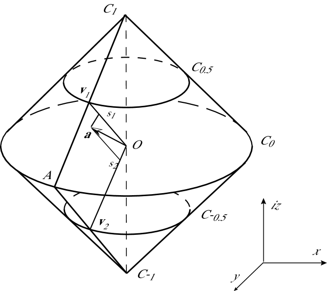
Figure 1: The domain $D_{1}$ obtained by intersecting $D_{s,n}$ with the subspace $M_{1}=\{(x,y,iz):\;x,y,z\in R\}.$ $D_{1}$ is the intersection of two circular cones. The minimal tripotents belong to two circles $C_{0.5}$ and $C_{-0.5}$, whose respective equations are $iz=0.5$ and $iz=-0.5$ . The maximal tripotents are the two points $C_{1}=(0,0,i)$ and $C_{-1}=(0,0,-i),$ as well as the points of the circle $C_{0}$: $iz=0$ . The norm-exposed faces are either points or line segments.

To locate the minimal tripotents $\mathbf{v}$ in $D_{1}$, we introduce polar coordinates $r,\theta$ in the $x$-$y$ plane. Then $\mathbf{v}=(r\cos\theta,r\sin\theta,iz,0,...).$ The conditions $\det\mathbf{v}=0$ and $|Re(\mathbf{v})|=|Im(\mathbf{v})|=1/2$ imply that

$$\mathbf{v}=1/2(\cos\theta,\sin\theta,\pm i),$$ (47)

so the minimal tripotents lie on two circles $C_{0.5}$ and $C_{-0.5}$ of radius 1/2. Maximal tripotents are multiples of a real vector of unit length. Thus, the maximal tripotents of $D_{1}$ are $C_{1}=(0,0,i,)$, and $C_{-1}=(0,0,-i)$ and the circle $C_{0}=\{(\cos\theta,\sin\theta,0):\theta\in R\}$ of radius 1.

We can now visualize the geometry of the singular decomposition. Let $\mathbf{a}=(r\cos\theta,r\sin\theta,iz)$ and let $r>z>0.$ The minimal tripotents in the singular decomposition of $\mathbf{a}$ are

$$\mathbf{v}_{1}=1/2(\cos\theta,\sin\theta,i),\;\;\mathbf{v}_{2}=1/2(\cos\theta,\sin\theta,-i).$$

These tripotents are the intersection of the plane through $\mathbf{a}$, $C_{1}$ and $C_{-1}$ with the circles $C_{0.5}$ and $C_{-0.5}$ of minimal tripotents . The singular numbers of $\mathbf{a}$ are $s_{1}=r+z$ and $s_{2}=r-z.$ Thus the singular decomposition of $\mathbf{a}$ is

$$\mathbf{a}=\frac{r+z}{2}(\cos\theta,\sin\theta,i)+\frac{r-z}{2}(\cos\theta,\sin\theta,-i).$$

See Figure 1.

6 The homogeneity of the unit ball of $\mathcal{S}^{n}$

Let $D$ be a domain in a complex linear space $X$. A map $\xi:D\rightarrow X$ is called a vector field on $D$. We will say that a vector field $\xi$ is analytic if, for any point $\mathbf{z}\in D,$ there is a neighborhood of $\mathbf{z}$ in which $\xi$ is the sum of a power series. A well-known theorem from the theory of differential equations states that if $\xi$ is an analytic vector field on $D$ and $\mathbf{z}\in D,$ then the initial-value problem

$$\frac{d\mathbf{w}(\tau)}{d\tau}=\xi(\mathbf{w}(\tau)),\;\;\;\mathbf{w}(0)=\mathbf{z}$$ (48)

has a unique solution for real $\tau$ in some neighborhood of $\tau=0.$ A analytic vector field $\xi$ is called a complete if for any $\mathbf{z}\in D$ the solution of the initial-value problem (48) exists for all real $\tau$ and $\mathbf{w}(\tau)\in D.$

For each $\mathbf{a}\in\mathcal{S}^{n},$ we define a vector field representing a generator of translation, by

$$\xi_{\mathbf{a}}(\mathbf{w})=\mathbf{a}-\{\mathbf{w},\mathbf{a},\mathbf{w}\}.\;\;$$ (49)

Note that $\xi_{\mathbf{a}}$ is a second-degree polynomial in $\mathbf{w}$ and, thus, an analytic vector field. Since $\xi_{\mathbf{a}}$ is tangent on the boundary of $D_{s,n},$ the solution of (48) exists for any real $\tau$. This solution generates an analytic map defined by $\exp(\xi_{\mathbf{a}}\tau)(\mathbf{z})=\mathbf{w}(\tau)$ for any $\mathbf{z}\in D_{s,n},$ where $\mathbf{w}(\tau)$ denote a solution of (48) with $\xi=\xi_{\mathbf{a}}$.

For any given $\mathbf{b}\in D_{s,n}$ with the singular decomposition $\mathbf{b}=s_{1}\mathbf{v}_{1}+s_{2}\mathbf{v}_{2}$, let $\mathbf{a}=\tanh^{-1}(s_{1})\mathbf{v}_{1}+\tanh^{-1}(s_{2})\mathbf{v}_{2},$ then $\exp(\xi_{\mathbf{a}})(\mathbf{0})=\mathbf{b}.$ This show that the origin in domain $D_{s,n}$ can be moved to any point $\mathbf{b}\in D_{s,n}$ by an analytic automorphism of this domain. This property of a domain is called homgeneouity of the domain.

Since $D_{s,n}$ is the unit ball in the operator norm, the reflection map $\mathbf{w}\to-\mathbf{w}$ is an analytic symmetry on $D_{s,n}$ which fixes only the origin. Clearly, $D_{s,n}$ is bounded. Since $D_{s,n}$ is homogeneous, it is a bounded symmetric domain, meaning that for any $\mathbf{a}\in D_{s,n}$, there is an analytic automorphism $s_{\mathbf{a}}$ which is a symmetry (i.e. $s_{\mathbf{a}}^{2}=id$) and fixes only the point $\mathbf{a}$. It is known that any bounded symmetric domain define uniquely a triple product for which the generators of translations are given by (49). Thus, the spin triple product is defined uniquely by the domain $D_{s,n}$.

For any pair of points $\mathbf{a},\mathbf{b}$ in a bounded symmetric domain there is an operator, called the Bergman operator, defined as

$$B(\mathbf{a},\mathbf{b})=I-2D(\mathbf{a},\mathbf{b})+Q(\mathbf{a})Q(\mathbf{b}).$$ (50)

It can be shown [11] that for any $\mathbf{a}\in D_{s,n}$ the operator $B(\mathbf{a},\mathbf{a})$ is invertible and the invariant metric on $D_{s,n}$ at $\mathbf{a}$ is given by:

$$h_{\mathbf{a}}(\mathbf{x},\mathbf{y})=\langle B(\mathbf{a},\mathbf{a})^{-1}\mathbf{x}|\mathbf{y}\rangle$$ (51)

for any $\mathbf{x},\mathbf{y}\in\mathcal{S}^{n}$, which can be considered as the tangent space to $D_{s,n}$ at $\mathbf{a}$. The curvature tensor of this metric at 0 is given by

$$R_{0}(\mathbf{x},\mathbf{y})=D(\mathbf{y},\mathbf{x})-D(\mathbf{x},\mathbf{y}).$$ (52)

7 Geometry of the dual ball of the spin factor

Every normed linear space $A$ over the complex numbers equipped with a norm has a dual space, denoted $A^{*},$ consisting of complex linear functionals, i.e., linear maps from $A$ to the complex numbers. We define a norm on $A^{*}$ by

$$\|f\|_{*}=\sup\{|f(\mathbf{w})|:\;\mathbf{w}\in A,\|\mathbf{w}\|\leq 1\}.$$ (53)

The dual (or predual) of $\mathcal{S}^{n}$ is the set of complex linear functionals on $\mathcal{S}^{n}$. We denote it by $\mathcal{S}^{n}_{*}.$

We use the inner product on $\mathbf{C}^{n}$ to define an imbedding of $\mathcal{S}^{n}$ into $\mathcal{S}^{n}_{*},$ as follows. For any element $\mathbf{a}\in\mathcal{S}^{n},$ we define a complex linear functional $\hat{\mathbf{a}}\in\mathcal{S}^{n}_{*}$ by

$$\hat{\mathbf{a}}(\mathbf{w})=\langle\mathbf{w}|2\mathbf{a}\rangle.$$ (54)

The coefficient 2 of $\mathbf{a}$ is needed to make the dual of a minimal tripotent have norm 1. Conversely, for any $\mathbf{f}\in\mathcal{S}^{n}_{*},$ there is an element $\check{\mathbf{f}}\in\mathcal{S}^{n}$ such that for all $\mathbf{w}\in\mathcal{S}^{n},$

$$\mathbf{f}(\mathbf{w})=\langle\mathbf{w}|2\check{\mathbf{f}}\rangle.$$ (55)

The above (53) norm on $\mathcal{S}^{n}_{*}$ is called the trace norm and is as follows. Let $\mathbf{f}\in\mathcal{S}^{n}_{*}$. Suppose that $\check{\mathbf{f}}$ has the singular decomposition (35) $\check{\mathbf{f}}=s_{1}\mathbf{v_{1}}+s_{2}\mathbf{v}_{2}$. It can then, be shown that

$$\|\mathbf{f}\|_{*}=s_{1}+s_{2}=\sqrt{2|\check{\mathbf{f}}|^{2}+2|\det\check{\mathbf{f}}|}.$$ (56)

From this, it follows that if $\mathbf{f}\in\mathcal{S}^{n}_{*}$ has trace norm one, then

$$\mathbf{f}=s_{1}\hat{\mathbf{v}}_{1}+s_{2}\hat{\mathbf{v}}_{2},\;\;s_{1},s_{2}\geq 0,\;s_{1}+s_{2}=1,$$ (57)

meaning that any norm one state is a convex combination of two algebraically orthogonal extreme states, which correspond to pure states in quantum mechanics.

The unit ball $S_{n}$ in $\mathcal{S}^{n}_{*}$ is defined by

$$S_{n}=\{\mathbf{f}\in\mathcal{S}^{n}_{*}:\;\|\mathbf{f}\|_{*}\leq 1\}.$$ (58)

We call the ball $S_{n}$ the state space of $\mathcal{S}^{n}.$ To understand the geometry of this ball, we will examine the three-dimensional section $D^{*}_{1}$ consisting of those elements $\mathbf{f}\in S_{n}$ satisfying

$$2\check{\mathbf{f}}\in M_{1}=\{(x,y,iz):\;\;\;x,y,z\in R\}.$$ (59)

It can be shown that

$$D^{*}_{1}=\{(x,y,iz):\;\;\max\{\sqrt{x^{2}+y^{2}},\,|z|\}\leq 1\},$$

which is a cylinder (see Figure 2).

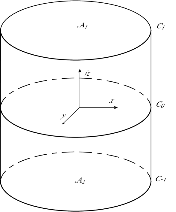
Figure 2: The domain $D^{*}_{1}$ obtained by intersecting the state space $S_{n}$ with the subspace $M_{1}=\{(x,y,iz):\;\;\;x,y,z\in R\}.$ $D^{*}_{1}$ is a cylinder. The pure states, corresponding to minimal tripotents, are extreme points of the domain and belong to two unit circles $C_{1}:iz=1$ and $C_{-1}:iz=-1$. The functionals corresponding to maximal tripotents are $A_{1}=(0,0,i)$ and $A_{2}=(0,0,-i)$ and each point of the circle $C_{0}:iz=0.$ They are centers of faces. The norm-exposed faces are either points, line segments or disks.

To describe the functionals $\mathbf{f}$ in $D^{*}_{1}$ which correspond to minimal tripotents $\mathbf{v}=\check{\mathbf{f}},$ we introduce polar coordinates $r,\theta$ in the $x$-$y$ plane. For such functionals, by (47) we have

$$2\check{\mathbf{f}}=(\cos\theta,\sin\theta,\pm i),$$ (60)

yielding two circles $C_{1}$ and $C_{-1}$ of radius 1. The functionals corresponding to multiples of maximal tripotents are multiples of a real vector of unit length. Thus, the norm one functionals corresponding to multiples of maximal tripotents are $A_{1}=(0,0,i),$ $A_{2}=(0,0,-i),$ which are the centers of the two-dimensional discs of $\partial S_{n}$ and the center of the circle $C_{0}=(\cos\theta,\sin\theta,0)$ of radius 1. See Figure 2.

8 The state space of two-state systems

We will now apply the results of the previous section to represent the states of quantum mechanic systems. We will assume that the state space $S$ is a unit ball of a Banach space, which we will denote by $X_{*}$. We will consider only the geometry of the state space that is implied by the measuring process for quantum systems. Recall that the state space consists of two types of points. The first type represents mixed states, which can be considered as a mixture of other states with certain probabilities. The second type represents pure states, those states which cannot be decomposed as a mixture of other states. By definition, a pure state is an extreme point of the state space $S.$

A physical quantity which can be measured by an experiment is called an observable. The observables can be represented as linear functionals $\mathbf{a}\in X$ on the state space. This representation is obtained by assigning to each state $\mathbf{f}\in S$ the expected value of the physical quantity $\mathbf{a}$ when the system is in state $\mathbf{f}.$ A measurement causes the quantum system to move into an eigenstate of the observable that is being measured. Thus, the measuring process defines, for any set $\Delta$ of possible values of the observable $\mathbf{a}$, a projection $P_{\mathbf{a}}(\Delta)$ on the state space, called a filtering projection. The projection $P_{\mathbf{a}}(\Delta)$ represents a filtering device, called also a filter, that will move any state $\mathbf{f}$ to the state $P_{\mathbf{a}}(\Delta)\mathbf{f},$ for which the value of $\mathbf{a}$ is definitely in the set $\Delta$ and the probability of passing this filter is $\|P_{\mathbf{a}}(\Delta)\mathbf{f}\|/\|\mathbf{f}\|.$

Since, applying the filter a second time will not affect the output state after the first application of the filter, $P_{\mathbf{a}}(\Delta)$ is a projection. It is assumed that if the value of $\mathbf{a}$ on the state $\mathbf{f}$ was definitely in $\Delta,$ then the filtering projection does not change the state $\mathbf{f}.$ Such a projection is called neutral.

A norm-exposed face of the unit ball $S$ of $X_{*}$ is a non-empty subset of $S$ of the form

$$F_{\mathbf{x}}=\{\mathbf{f}\in S:\mathbf{f}(\mathbf{x})=1\},$$ (61)

where $\mathbf{x}\in X,\|\mathbf{x}\|=1$. Recall that a face $G$ of a convex set $K$ is a non-empty convex subset of $K$ such that if $\mathbf{g}\in G$ and $\mathbf{h},\mathbf{k}\in K$ satisfy $\mathbf{g}=\lambda\mathbf{h}+(1-\lambda)\mathbf{k}$ for some $\lambda\in(0,1)$, then $\mathbf{h},\mathbf{k}\in G$. We say that two states $\mathbf{f},\mathbf{g}$ are orthogonal if $\|\mathbf{f}+\mathbf{g}\|=\|\mathbf{f}-\mathbf{g}\|=\|\mathbf{f}\|+\|\mathbf{g}\|.$ For any subset $A$, $A^{\Diamond}$ denotes the set of all elements which are orthogonal to every element of $A.$ An element $\mathbf{u}\in X$ is called a projective unit if $\|\mathbf{u}\|=1$ and $\mathbf{u}(F_{\mathbf{u}}^{\Diamond})=0$.

Motivated by the measuring processes in quantum mechanics, we define a symmetric face to be a norm-exposed face $F$ in $S$ with the following property: there is a linear isometry $S_{F}$ of $X_{*}$ onto $X_{*}$ which is a symmetry, i.e., $S_{F}^{2}=I$, such that $\|S_{F}\|=1$ and the fixed point set of $S_{F}$ is $(\overline{\mbox{sp}}F)\oplus F^{\Diamond}$. The map $S_{F}$ is called the facial symmetry associated with $F$. A complex normed space $X_{*}$ is said to be weakly facially symmetric if every norm-exposed face in $S$ is symmetric. A weakly facially symmetric space $X_{*}$ is also strongly facially symmetric if for every norm-exposed face $F$ in $S$ and every $\mathbf{y}\in X$ with $\|\mathbf{y}\|=1$ and $F\subset F_{\mathbf{y}}$, we have $S_{F}^{*}\mathbf{y}=\mathbf{y}$.

For each symmetric face $F$, we define contractive projections $P_{k}(F),\ k=0,1/2,1$, on $X_{*}$ as follows. First, $P_{1/2}(F)=(I-S_{F})/2$ is the projection on the $-1$ eigenspace of $S_{F}$. Next, we define $P_{1}(F)$ and $P_{0}(F)$ as the projections of $X_{*}$ onto $\overline{\mbox{sp}}F$ and $F^{\Diamond}$, respectively, so that $P_{1}(F)+P_{0}(F)=(I+S_{F})/2$. A normed space $X_{*}$ is called neutral if for every symmetric face $F$, the projection $P_{1}(F)$ is neutral, meaning that

$$\|P_{1}(F)\mathbf{f}\|=\|\mathbf{f}\|\;\Rightarrow\;P_{1}(F)\mathbf{f}=\mathbf{f}$$

for any $\mathbf{f}\in X_{*}.$ In such spaces there is a one-to-one correspondence between projective units and norm-exposed faces.

In a neutral strongly facially symmetric space $X_{*}$, for any non-zero element $\mathbf{f}\in X_{*}$, there exists a unique projective unit $\mathbf{v}=\mathbf{v}(\mathbf{f}),$ called the support tripotent, such that $\mathbf{f}(\mathbf{v})=\|\mathbf{f}\|$ and $\mathbf{v}(\{\mathbf{f}\}^{\Diamond})=0.$ The support tripotent $\mathbf{v}(\mathbf{f})$ is a minimal projective unit if and only if $\mathbf{f}/\|\mathbf{f}\|$ is an extreme point of the unit ball of $X_{*}$.

Let $\mathbf{f}$ and $\mathbf{g}$ be extreme points of the unit ball of a neutral strongly facially symmetric space $X_{*}$. The transition probability of $\mathbf{f}$ and $\mathbf{g}$ is the number

$$\langle\mathbf{f}|\mathbf{g}\rangle:=\mathbf{f}(\mathbf{v}(\mathbf{g})).$$

A neutral strongly facially symmetric space $X_{*}$ is said to satisfy “symmetry of transition probabilities” (STP) if for every pair of extreme points $\mathbf{f},\mathbf{g}\in S$, we have

$$\overline{\langle\mathbf{f}|\mathbf{g}\rangle}=\langle\mathbf{g}|\mathbf{f}\rangle,$$

where in the case of complex scalars, the bar denotes conjugation. We define the rank of a strongly facially symmetric space $X_{*}$ to be the maximal number of orthogonal projective units.

The two-state quantum systems are systems on which any measurement can not give more than two different results. The state space of such systems is of rank 2. In [7] it was shown that if $X_{*}$ is a rank 2 neutral strongly facially symmetric space satisfying STP, then $X_{*}$ is linearly isometric to the predual of a spin factor.

9 Spin grid of $\mathcal{S}^{4}$ and Pauli matrices

Let $\{\mathbf{u}_{0},\mathbf{u}_{1},\mathbf{u}_{2},\mathbf{u}_{3}\}$ be an arbitrary TCAR basis in $\mathcal{S}^{4}.$ Then from (25) it follows that

$$\mathbf{v}=0.5(\mathbf{u}_{0}+i\mathbf{u}_{1})=0.5(1,i,0,0),\;\;\overline{\mathbf{v}}=0.5(\mathbf{u}_{0}-i\mathbf{u}_{1})=0.5(1,-i,0,0)$$ (62)

are a pair of algebraically orthogonal minimal tripotents. Note that $\mathcal{S}^{4}_{1/2}(\mathbf{v})$ from the Peirce decomposition (30) with respect to $\mathbf{v}$ has dimension 2. Also,

$$\mathbf{w}=0.5(\mathbf{u}_{2}+i\mathbf{u}_{3})=0.5(0,0,1,i),\;\;\overline{\mathbf{w}}=0.5(\mathbf{u}_{2}-i\mathbf{u}_{3})=0.5(0,0,1,-i)$$ (63)

are a pair of algebraically orthogonal minimal tripotents in $\mathcal{S}^{4}_{1/2}(\mathbf{v})$.

The set $\{\mathbf{v},\overline{\mathbf{v}},\mathbf{w},\overline{\mathbf{w}}\}$ is a basis of $\mathcal{S}^{4}$ consisting of minimal tripotents. It is an example of a spin grid, which we will define now. We say that a collection of tripotents is compatible if the collection of all Pierce projections associated with this family commute. We say that a collection of four elements $(\mathbf{v},\overline{\mathbf{v}};\mathbf{w},\overline{\mathbf{w}})$ (composed of two pairs) in $\mathcal{S}^{4}$ form a spin grid if the following relations hold:

• $\mathbf{v},\mathbf{w},\overline{\mathbf{v}},\overline{\mathbf{w}}$ are minimal compatible tripotents,

• the pairs $(\mathbf{v},\overline{\mathbf{v}})$ and $(\mathbf{w},\overline{\mathbf{w}})$ are algebraically orthogonal,

• the pairs $(\mathbf{v},\mathbf{w}),(\mathbf{v},\overline{\mathbf{w}}),(\mathbf{w},\overline{\mathbf{v}})$ and $(\overline{\mathbf{w}},\overline{\mathbf{v}})$ are co-orthogonal (the pair $(\mathbf{v},\mathbf{w})$ is said to be co-orthogonal if $D(\mathbf{v},\mathbf{v})\mathbf{w}=0.5\mathbf{w}$ and $D(\mathbf{w},\mathbf{w})\mathbf{v}=0.5\mathbf{v}$),

• $\{\mathbf{w},\mathbf{v},\overline{\mathbf{w}}\}=-0.5\overline{\mathbf{v}}$ and $\{\mathbf{v},\mathbf{w},\overline{\mathbf{v}}\}=-0.5\overline{\mathbf{w}}.$

The spin grid in $\mathcal{S}^{4}$ is also called an odd quadrangle.

The following $2\times 2$ elementary matrices

$$\mathbf{v}=\begin{pmatrix}1&0\\ 0&0\ \end{pmatrix},\overline{\mathbf{v}}=\begin{pmatrix}0&0\\ 0&1\ \end{pmatrix},\mathbf{w}=\begin{pmatrix}0&1\\ 0&0\ \end{pmatrix},\overline{\mathbf{w}}=\begin{pmatrix}0&0\\ -1&0\ \end{pmatrix},$$ (64)

with the triple product

$$\{a,b,c\}=\frac{ab^{*}c+cb^{*}a}{2}$$ (65)

are an example of an odd quadrangle. They are isomorphic to the spin grid in $\mathcal{S}^{4}$. Their complex span is isomorphic to the space of $2\times 2$ complex matrices, which now can be used to represent the triple product in $\mathcal{S}^{4}$. The minus sign in $\overline{\mathbf{w}}$ is needed in order that the quadrangle will be an odd one.

Since $\mathbf{u}_{0}=\mathbf{v}+\overline{\mathbf{v}}$, $\mathbf{u}_{1}=i(\overline{\mathbf{v}}-\mathbf{v})$, $\mathbf{u}_{2}=\mathbf{w}+\overline{\mathbf{w}}$ and $\mathbf{u}_{3}=i(\overline{\mathbf{w}}-\mathbf{w})$, the TCAR basis of $\mathcal{S}^{4}$ $\{\mathbf{u}_{1},\mathbf{u}_{2},\mathbf{u}_{3},\mathbf{u}_{4}\}$ in this representation becomes

$$\mathbf{u}_{0}=\begin{pmatrix}1&0\\ 0&1\ \end{pmatrix},\mathbf{u}_{1}=\begin{pmatrix}-i&0\\ 0&i\ \end{pmatrix},\mathbf{u}_{2}=\begin{pmatrix}0&1\\ -1&0\ \end{pmatrix},\mathbf{u}_{3}=\begin{pmatrix}0&-i\\ -i&0\ \end{pmatrix}.$$

Note that

$$\mathbf{u}_{0}=I,\mathbf{u}_{1}=-i\sigma_{3},\mathbf{u}_{2}=-i\sigma_{2},\mathbf{u}_{3}=-i\sigma_{1},$$ (66)

where $\sigma_{j}$ denote the Pauli matrices. Conversely, the elements of the spin grid $\mathbf{v}=0.5(\mathbf{u}_{0}+i\mathbf{u}_{1})$ and $\overline{\mathbf{v}}=0.5(\mathbf{u}_{0}-i\mathbf{u}_{1})$ are obtained from the TCAR basis by formulas similar to the creation and annihilation operators in quantum field theory.

Any element $\mathbf{a}=(a_{0},a_{1},a_{2},a_{3})\in\mathcal{S}^{4}$ can be represented by a $2\times 2$ matrix $A$ as

$$\sum^{4}_{j=1}a_{j}\,\mathbf{u}_{j}=\begin{pmatrix}a_{0}-ia_{1}&a_{2}-ia_{3}\\ -a_{2}-ia_{3}&a_{0}+ia_{1}\end{pmatrix}=A.$$

Note that

$$\det A=a_{0}^{2}+a_{1}^{2}+a_{2}^{2}+a_{3}^{2}=\det\mathbf{a},$$ (67)

providing another justification for the definition of the determinant in the spin factor.

For a spin factor $\mathcal{S}^{n}$ of any dimension, the spin grid basis is constructed from odd quadrangles and each pair of quadrangles is glued by the diagonal. We will demonstrate this on the spin factor $\mathcal{S}^{6}$, which will play an important role later. The grid of $\mathcal{S}^{6}$ can be represented by 6 (coming in 3 pairs) elementary $4\times 4$ antisymmetric matrices:

$$\{\mathbf{e}_{01},\mathbf{e}_{23};\mathbf{e}_{02},\mathbf{e}_{31};\mathbf{e}_{03},\mathbf{e}_{12}\},$$

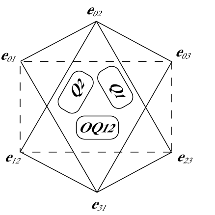
where $\mathbf{e}_{kl}$ could be identified with $D(\mathbf{u}_{k},\mathbf{u}_{l})$ as an operator on $\mathcal{S}^{4}$. The spin grid consists of 3 odd quadrangles : $(\mathbf{e}_{01},\mathbf{e}_{23};\mathbf{e}_{02},\mathbf{e}_{31}),$ $(\mathbf{e}_{02},\mathbf{e}_{31};\mathbf{e}_{03},\mathbf{e}_{12})$ and $(\mathbf{e}_{01},\mathbf{e}_{23};\mathbf{e}_{03},\mathbf{e}_{12})$ glued by the diagonal (a common pair), as seen on Figure 3. Note that we had to use $\mathbf{e}_{31}=-\mathbf{e}_{13}$ to make all the quadrangles odd.

Figure 3: Two quadrangles $\mathbf{Q}1$ and $\mathbf{Q}2$ glued by the diagonal. Here, $(\mathbf{e}_{01},\mathbf{e}_{23};\mathbf{e}_{03},\mathbf{e}_{12})$ form an odd quadrangle, denoted $\mathbf{OQ}12$.

10 The spin 1 Lorentz group representation on $\mathcal{S}^{4}$

It is known that the transformation of the electromagnetic field strength $\mathbf{E},\mathbf{B}$ from one inertial system to another preserves the complex quantity $\mathbf{F}^{2},$ where $\mathbf{F}=\mathbf{E}+ic\mathbf{B}.$ If we consider $\mathbf{F}$ as an element of $\mathcal{S}^{3},$ then $\mathbf{F}^{2}=\det\mathbf{F}.$ Thus, if we take $\mathcal{S}^{3}$ as the space representing the set of all possible electromagnetic field strengths, then the Lorentz group acts on $\mathcal{S}^{3}$ by linear transformations which preserve the determinant. This leads us to study the Lie group of determinant-preserving linear maps on $\mathcal{S}^{3}$ (and, in general, on $\mathcal{S}^{n}$) and the Lie algebra of this group.

Let $\mbox{Dinv}\,(\mathcal{S}^{n})$ denote the group of all invertible linear maps $\mathcal{S}^{n}\rightarrow\mathcal{S}^{n}$ which preserve the determinant and let $\mbox{dinv}\,(\mathcal{S}^{n})$ denote the Lie algebra of $\mbox{Dinv}\,(\mathcal{S}^{n})$. It can be shown that $\mbox{dinv}\,(\mathcal{S}^{n})\subset A_{n}({C}),$ where $A_{n}({C})$ denotes the space of all $n\times n$ complex antisymmetric matrices. Using the triple product on $\mathcal{S}^{n}$, we can express this Lie algebra as

$$\mbox{dinv}\,(\mathcal{S}^{n})=\{\sum_{k<l}d_{kl}D(\mathbf{u}_{k},\mathbf{u}_{l}):\;\>d_{kl}\in C\}.$$ (68)

We define now a spin 1 representation of the Lorentz group by elements of $\mbox{Dinv}\,(\mathcal{S}^{4}).$ Let $J_{1},J_{2},J_{3},K_{1},K_{2},K_{3}$ denote the standard infinitesimal generators of rotations and boosts respectively, in the Lorentz Lie algebra. Furthermore, let $\mathbf{u}_{0},\mathbf{u}_{1},\mathbf{u}_{2},\mathbf{u}_{3}$ denote a TCAR basis of $\mathcal{S}^{4}$. We will define a representation $\pi_{s}^{4}$ of the Lorentz Lie algebra by elements of $\mbox{dinv}\,(\mathcal{S}^{4}).$ For ease of notation, we shall write $D_{jk}$ instead of $D(\mathbf{u}_{j},\mathbf{u}_{k}),$ for $j,k\in\{0,1,2,3\},$ $j\neq k.$ We have seen earlier that $D_{23}=D(\mathbf{u}_{2},\mathbf{u}_{3})$ generates a rotation around the $x$-axis. Thus, we define $\pi_{s}^{4}$ by

$$\pi_{s}^{4}(J_{1})=D_{23},\;\pi_{s}^{4}(J_{2})=D_{31},\;\pi_{s}^{4}(J_{3})=D_{12}.$$ (69)

Since $K_{1}$, the generator of a boost in the $x$-direction, perform both an $x$-coordinate space change of the moving frame and also a time change due to the relative speed between the frames, it is natural to define

$$\pi_{s}^{4}(K_{1})=iD_{01},\;\pi_{s}^{4}(K_{2})=iD_{02},\;\pi_{s}^{4}(K_{3})=iD_{03}.$$ (70)

The coefficient $i$ is needed to satisfy the commutation relations.

It is easy to show that the commutation relations of the Lorentz algebra are satisfied. The representation of the Lorentz group by elements of $\mbox{Dinv}\,(\mathcal{S}^{4})$ is now obtained by taking the exponent of the basic elements of $\pi_{s}^{4}.$

It is easy to check that the subspace

$$M_{1}=\{(x^{0},x^{1},x^{2},x^{3})=x^{\nu}\mathbf{u}_{\nu}\in\mathcal{S}^{4}:\;\;x^{0}\in R,\;\;x^{1},x^{2},x^{3}\in iR\}$$ (71)

is invariant under $\pi_{s}^{4}.$ We can attach the following meaning to the subspace $M_{1}.$ Let $M$ be the Minkowski space representing the space-time coordinates $(t,x,y,z)$ of an event in an inertial system. Define a map $\Psi:M\to M_{1}$ by

$$\Psi(t,x,y,z)=ct\mathbf{u}_{0}-ix\mathbf{u}_{1}-iy\mathbf{u}_{2}-iz\mathbf{u}_{3}.$$ (72)

We use the minus sign for the space coordinates in order that the resulting Lorentz transformations will have their usual form. Note that

$$\det(\Psi(t,x,y,z))=(ct)^{2}-x^{2}-y^{2}-z^{2}=s^{2},$$

where $s$ is the space-time interval.

Any map $T\in\mbox{Dinv}\,(\mathcal{S}^{4})$ which maps $M_{1}$ into itself generates an interval-preserving map

$$\Lambda=\Psi^{-1}T\Psi$$ (73)

from $M$ to $M$. Thus, any map $T$ from $\pi_{s}^{4}$ generates by (73) a space-time Lorentz transformation. For example, consider the Lorentz transformation generated by a boost $K_{1}$ in the $x$-direction. Obviously, such transformation changes the $x$-coordinate and the time and do not change $y,z$-coordinates. Direct calculation show that if $T=\exp\varphi\pi_{s}^{4}(K_{1})$, then

$$\Lambda(t,x,y,z)=\left(\begin{array}[]{cccc}\cosh\varphi&c^{-1}\sinh\varphi&0&0\\ c\sinh\varphi&\cosh\varphi&0&0\\ 0&0&1&0\\ 0&0&0&1\end{array}\right)\left(\begin{array}[]{c}t\\ x\\ y\\ z\end{array}\right),$$

which is the usual Lorentz space-time transformation for the boost in the $x$-direction, where $\tanh\varphi=\mathbf{v}/c,$ and $\mathbf{v}$ is the relative velocity between the systems. Conversely, any space-time Lorentz transformation $\Lambda$ generates a transformation $T=\Psi\Lambda\Psi^{-1}$ on $M_{1}$ which can be extended linearly to a map on $\mathcal{S}^{4}$ which belongs to $\pi_{s}^{4}.$ Thus, the usual Lorentz space-time transformation is equivalent to a representation $\pi_{s}^{4},$ and $\pi_{s}^{4}$ can be considered as an extension of the usual representation of the Lorentz group from space-time to $\mathcal{S}^{4}.$

In addition to the subspace $M_{1},$ the representation $\pi_{s}^{4}$ preserves the subspace

$$M_{2}=\{(p_{0},p_{1},p_{2},p_{3})=p_{\nu}\mathbf{u}_{\nu}\in\mathcal{S}^{4}:\;\;p_{0}\in iR,\;\;p_{1},p_{2},p_{3}\in R\},$$ (74)

which is complementary to $M_{1}.$ We can attach the following meaning to the subspace $M_{2}.$ Let $\widetilde{M}$ be the Minkovski space representing the four-vector momentum $(p_{0},p_{1},p_{2},p_{3})=m_{0}(c\gamma,\gamma\mathbf{v}),$ where $m_{0}$ is the rest-mass and $(\gamma,\gamma\mathbf{v}/c)$ is the four-velocity of the object. Define a map $\widetilde{\Psi}:\widetilde{M}\to M_{2}$ by

$$\widetilde{\Psi}(p_{0},p_{1},p_{2},p_{3})=i\,p_{0}\mathbf{u}_{0}+p_{1}\mathbf{u}_{1}+p_{2}\mathbf{u}_{2}+p_{3}\mathbf{u}_{3}.$$ (75)

Note that

$$\det(\widetilde{\Psi}(p_{0},p_{1},p_{2},p_{3}))=-p_{0}^{2}+p_{1}^{2}+p_{2}^{2}+p_{3}^{2}=-(E/c)^{2}+\mathbf{p}^{2}=-(m_{0}c)^{2}$$

is invariant under the Lorentz transformations.

Any linear map $T$ on $\mathcal{S}^{4}$ which maps $M_{2}$ into itself generates a map

$$T|_{\widetilde{M}}=\widetilde{\Psi}^{-1}T\widetilde{\Psi}$$ (76)

from $\widetilde{M}$ to $\widetilde{M}$. If $T\in\mbox{Dinv}\,(\mathcal{S}^{4})$, then the map $T|_{\widetilde{M}}$ is a Lorentz transformation on the four-vector momentum space. It can be shown that any Lorentz four-vector momentum transformation is equivalent to an element of the representation $\pi_{s}^{4},$ and $\pi_{s}^{4}$ can be considered as an extension of the usual representation of the Lorentz group from four-vector momentum space to $\mathcal{S}^{4}.$

The electromagnetic field $\bf{E,B}$ on $\widetilde{M}$ is represented by

$$\mathbf{F}=E_{k}\pi_{s}^{4}(K_{k})|_{\widetilde{M}}+cB_{k}\pi_{s}^{4}(J_{k})|_{\widetilde{M}}=$$

$$\left(\begin{array}[]{cccc}0&E_{1}&E_{2}&E_{3}\\ -E_{1}&0&cB_{3}&-cB_{2}\\ -E_{2}&-cB_{3}&0&cB_{1}\\ -E_{3}&cB_{2}&-cB_{1}&0\end{array}\right),$$ (77)

which is representation of the field by the electro-magnetic field tensor. This is very natural, since the electric field generates boosts and the magnetic field generates rotations.

In classical mechanics, we use the phase space, consisting of position and momentum, to describe the state of a system. The properties of the representation $\pi_{s}^{4}$ suggest that $\mathcal{S}^{4}$ can serve as a relativistic analog of the phase space by representing space-time and four-momentum on it. Note that any relativistically invariant multiple of four-momentum can be used instead of four-momentum. For instance, we may use four-velocity instead of four-momentum. In order to allow transformations under which the subspaces $M_{1}$ and $M_{2}$ are not invariant, we have to multiply the four-momentum by a universal constant that will make the units of $M_{1}$ equal to the units of $M_{2}.$

We propose two models for $\mathcal{S}^{4}$ as the relativistic phase space:

1) The space-momentum model for the relativistic phase space:

$$\Omega(t,x,y,z,E/c,p_{1},p_{2},p_{3})=$$ (78)

$$(ct+\varsigma iE/c)\mathbf{u}_{0}+(\varsigma p_{1}-ix)\mathbf{u}_{1}+(\varsigma p_{2}-iy)\mathbf{u}_{2}+(\varsigma p_{3}-iz)\mathbf{u}_{3},$$

where the universal constant $\varsigma$ transforms momentum into length.

2) The space-velocity model for the relativistic phase space:

$$\widetilde{\Omega}(t,x,y,z,\gamma,\gamma\mathbf{v}_{1}/c,\gamma\mathbf{v}_{2}/c,\gamma\mathbf{v}_{3}/c)=$$ (79)

$$(ct+i\varpi\gamma)\mathbf{u}_{0}+(\varpi\gamma\mathbf{v}_{1}/c-ix)\mathbf{u}_{1}+(\varpi\gamma\mathbf{v}_{2}/c-iy)\mathbf{u}_{2}+(\varpi\gamma\mathbf{v}_{3}/c-iz)\mathbf{u}_{3},$$

where the universal constant $\varpi$ transforms velocity into length. A similar relativistic phase space, called “velocity phase spacetime” was used also in [12].

For example, the physical meaning of a multiple of the tripotent $\mathbf{u}=0.5(\mathbf{u}_{0}\pm i\mathbf{u}_{1})$ by a complex constant $\lambda$ in the space-momentum model satisfies:

$$\lambda\mathbf{u}=0.5\lambda(\mathbf{u}_{0}\pm i\mathbf{u}_{1})\Rightarrow m_{0}=0,\;x=\mp ct,\;p_{1}=\mp E/c,\;y=z=p_{2}=p_{3}=0.$$ (80)

and thus represents a particle with rest-mass $m_{0}=0$ moving with speed $c$ in the $x$-direction. Energy and momentum are expressed in terms of their wavelength. The $\lambda\mathbf{u}$ correspond also directed plane waves, see [2] (6.15).

11 The spin $\frac{1}{2}$ Lorentz group representations on $\mathcal{S}^{4}$

From (68), it follows that $\mbox{dinv}\,(\mathcal{S}^{4})$ coincides with the space $A_{4}(C)$ of $4\times 4$ antisymmetric matrices. As mentioned above, $A_{4}(C)$ with the triple product (65) is isomorphic to $\mathcal{S}^{6}$, the spin factor of dimension 6. The representation $\pi_{s}^{4},$ constructed in the previous section, uses minimal tripotents $\pi_{s}^{4}(J_{k})$ and $\pi_{s}^{4}(K_{k})$ of $\mbox{dinv}\,(\mathcal{S}^{4})\approx\mathcal{S}^{6}$ to represent the generators of rotations and boosts of the Lorentz group. These elements of $\mathcal{S}^{6}$ form a spin grid basis. The Lorentz group representations $\pi^{+}$ and $\pi^{-},$ defined below, use maximal tripotents which form a TCAR basis of $\mathcal{S}^{6}.$

Since for any $k,$ the generator of rotation $J_{k}$ commutes with the generator of a boost $K_{k}$ in the same direction, these operators must be represented by commuting elements in $\mathcal{S}^{6}.$ There are two possibilities for such commuting elements. The first one is to take algebraically orthogonal elements, as in the representation $\pi_{s}^{4},$ where $\pi_{s}^{4}(J_{k})$ and $\pi_{s}^{4}(K_{k})$ are algebraically orthogonal minimal tripotents in $\mathcal{S}^{6}.$ But there is another possibility - representing these generators by (complex) linearly dependent elements of $\mathcal{S}^{6}.$ More precisely, we will assume that $\pi^{+}(K_{k})=i\pi^{+}(J_{k})$ and $\pi^{-}(K_{k})=i\pi^{-}(J_{k}),$ for $k=1,2,3.$ Under these assumptions, if the representation of the rotations satisfy the commutation relations for the generators of rotations, all other commutation relations of the Lorentz algebra will be satisfied automatically.

We define the representation $\pi^{+}$ by

$$\pi^{+}(J_{1})=\frac{1}{2}(D_{01}+D_{23}),\;\pi^{+}(J_{2})=\frac{1}{2}(D_{02}+D_{31}),\;\pi^{+}(J_{3})=\frac{1}{2}(D_{03}+D_{12}).$$ (81)

The definition for the representation $\pi^{-}$ is similar:

$$\pi^{-}(J_{1})=\frac{1}{2}(D_{23}-D_{01}),\;\pi^{-}(J_{2})=\frac{1}{2}(D_{31}-D_{02}),\;\pi^{-}(J_{3})=\frac{1}{2}(D_{12}-D_{03}).$$ (82)

The constant $\frac{1}{2}$ is necessary in order to satisfy the commutation relations. For the representation $\pi^{+}$ the electromagnetic field is expressed by use of the Faraday $\mathbf{F}=\mathbf{E}+ic\mathbf{B}$ as

$$\mathbf{F}=iF_{k}\pi^{+}(J_{k})=\frac{i}{2}\left(\begin{array}[]{cccc}0&F_{1}&F_{2}&F_{3}\\ -F_{1}&0&F_{3}&-F_{2}\\ -F_{2}&-F_{3}&0&F_{1}\\ -F_{3}&F_{2}&-F_{1}&0\end{array}\right),$$ (83)

and similarly for the representation $\pi^{-}$.

Direct calculation shows that the multiplication table for $\pi^{+}(J_{k})$ is as in Table 2.

	$2\pi^{+}(J_{1})$	$2\pi^{+}(J_{2})$	$2\pi^{+}(J_{3})$
$2\pi^{+}(J_{1})$	$-I$	$-2\pi^{+}(J_{3})$	$2\pi^{+}(J_{2})$
$2\pi^{+}(J_{2})$	$2\pi^{+}(J_{3})$	$-I$	$-2\pi^{+}(J_{1})$
$2\pi^{+}(J_{3})$	$-2\pi^{+}(J_{2})$	$2\pi^{+}(J_{1})$	$-I$

Table 2: Multiplication table for $\pi^{+}(J_{k})$

The elements $\{2\pi^{+}(J_{1}),2\pi^{+}(J_{2}),2\pi^{+}(J_{3})\}$ and $\{2\pi^{-}(J_{1}),2\pi^{-}(J_{2}),2\pi^{-}(J_{3})\}$ satisfy TCAR as elements of the spin factor $\mathcal{S}^{6}.$ Moreover,

$$\{2\pi^{+}(J_{1}),2\pi^{+}(J_{2}),2\pi^{+}(J_{3}),2\pi^{-}(K_{1}),2\pi^{-}(K_{2}),2\pi^{-}(K_{3})\}$$ (84)

is a TCAR basis of $\mbox{dinv}\,(\mathcal{S}^{4})=A_{4}(C)=\mathcal{S}^{6}.$ By direct verification, we can show that the commutant of $\{\pi^{+}(J_{k}):k=1,2,3\}$ is $\mbox{sp}_{C}[\{\pi^{-}(J_{k}):k=1,2,3\}\cup\{I\}],$ which, when restricted to real scalars, is a four-dimensional associative algebra isomorphic to the quaternions. This can be seen by examining the multiplication table 2. The commutant of $\{\pi^{-}(J_{k}):k=1,2,3\}$ is $\mbox{sp}_{C}[\{\pi^{+}(J_{k}):k=1,2,3\}\cup\{I\}],$ which is also, after restriction to real scalars, isomorphic to the quaternions. Thus, the two representations $\pi^{+}$ and $\pi^{-}$ commute.

The above construction of the representations $\pi^{+}$ and $\pi^{-}$ from the representation $\pi_{s}^{4}$ can also be done via the Hodge operator, also called the star operator. The representation $\pi^{+}$ is then the skew-adjoint part of $\pi_{s}^{4}$ with respect to the Hodge operator, and the representation $\pi^{-}$ is the self-adjoint part of $\pi_{s}^{4}$ with respect to the Hodge operator.

Notice also that any operator of $\{\pi^{+}(J_{k}),\pi^{-}(J_{k}):k=1,2,3\}$ has two distinct eigenvalues, namely $\pm\frac{1}{2},$ implying that these representations are spin $\frac{1}{2}$ representations. This is also confirmed by direct calculation of the exponent of the generators of rotations. For example, in the TCAR basis $\{\mathbf{u}_{0},\mathbf{u}_{1},\mathbf{u}_{2},\mathbf{u}_{3}\}$ we have

$$R_{3}(\varphi)=\exp(\varphi\pi^{+}(J_{3}))=\left(\begin{array}[]{cccc}\cos\frac{\varphi}{2}&0&0&\sin\frac{\varphi}{2}\\ 0&\cos\frac{\varphi}{2}&\sin\frac{\varphi}{2}&0\\ 0&-\sin\frac{\varphi}{2}&\cos\frac{\varphi}{2}&0\\ -\sin\frac{\varphi}{2}&0&0&\cos\frac{\varphi}{2}\end{array}\right).$$

This shows that the angle of rotation in the representation is half of the actual angle of rotation.

It can be shown that the two subspaces

$$\Upsilon_{1}=\mbox{sp}_{C}\{\mathbf{v}_{1},\mathbf{v}_{2}\}\;\;\mbox{ and }\;\;\Upsilon_{2}=\mbox{sp}_{C}\{\mathbf{v}_{-1},\mathbf{v}_{-2}\},$$

where

$$\mathbf{v}_{\pm 1}=0.5(\mathbf{u}_{0}\pm i\mathbf{u}_{3}),\;\;\mathbf{v}_{\pm 2}=0.5(\mathbf{u}_{2}\pm i\mathbf{u}_{1}),$$

are invariant under the representation $\pi^{+}.$ Note that $\mathbf{v}_{1},\mathbf{v}_{2},\mathbf{v}_{-1},\mathbf{v}_{-2}$ form a basis in $\mathcal{S}^{4}$ consisting of minimal tripotents and form an odd quadrangle. The representation $\pi^{+}$ leaves both two-dimensional complex subspaces $\Upsilon_{1}$ and $\Upsilon_{2}$ invariant, and thus we obtain two two-dimensional representations of the Lorentz group. These representations are related to the Pauli matrices as follows:

$$\pi^{+}(J_{1})|_{\Upsilon_{1}}=i\sigma_{1},\;\;\pi^{+}(J_{2})|_{\Upsilon_{1}}=i\sigma_{2},\;\;\pi^{+}(J_{3})|_{\Upsilon_{1}}=i\sigma_{3},$$ (85)

and

$$\pi^{+}(J_{1})|_{\Upsilon_{2}}=-i\sigma_{1},\;\;\pi^{+}(J_{2})|_{\Upsilon_{2}}=i\sigma_{2},\;\;\pi^{+}(J_{3})|_{\Upsilon_{2}}=-i\sigma_{3}.$$ (86)

Hence, $\pi^{+}$ defines the usual spin $\frac{1}{2}$ representation on the subspace $\Upsilon_{1}$ via the Pauli matrices. This means that $\xi_{1}\mathbf{v}_{1}+\xi_{2}\mathbf{v}_{2}$ forms a spinor. On the subspace $\Upsilon_{2},$ the representation $\pi^{+}$ acts by complex conjugation on the usual spin $\frac{1}{2}$ representation. Hence $\eta_{1}\mathbf{v}_{-1}+\eta_{2}\mathbf{v}_{-2}$ forms a dotted spinor. This is similar to the action of the Lorentz group on Dirac bispinors, and so the basis $\{\mathbf{v}_{1},\mathbf{v}_{2},\mathbf{v}_{-1},\mathbf{v}_{-2}\}$ of $\mathcal{S}^{4}$ can serve as a basis for bispinors. Note that the TCAR basis $\{\mathbf{u}_{0},\mathbf{u}_{1},\mathbf{u}_{2},\mathbf{u}_{3}\}$, on the other hand, is a basis for four-vectors.

The two subspaces

$$\widetilde{\Upsilon}_{1}=\mbox{sp}_{C}\{\mathbf{v}_{-2},\mathbf{v}_{1}\}\;\;\mbox{ and }\;\;\widetilde{\Upsilon}_{2}=\mbox{sp}_{C}\{\mathbf{v}_{-1},\mathbf{v}_{2}\}$$

are invariant under the representation $\pi^{-}.$ Note that $\widetilde{\Upsilon}_{1},\widetilde{\Upsilon}_{2}$ are obtained from the same spin grid that was used for defining the invariant subspaces $\Upsilon_{1},\Upsilon_{2}$ of the representation $\pi^{+}.$ In both cases, the invariant subspaces are obtained by partitioning the set of four elements of the spin grid into two pairs of non-orthogonal tripotents. Both possible partitions are realized in the representations $\pi^{+}$ and $\pi^{-}.$ The restriction of $\pi^{-}$ to the invariant subspaces $\widetilde{\Upsilon}_{1}$ and $\widetilde{\Upsilon}_{2}$ leads to the same Pauli spin matrices as in (85) and (86). Thus, the representation $\pi^{-}$ is a direct sum of two complex conjugate copies of the spin $\frac{1}{2}$ two-dimensional representation given by the Pauli spin matrices. Hence, $\pi^{-}$ is also a representation of the Lorentz group on the Dirac bispinors.

We now lift the representations $\pi^{+}$ and $\pi^{-}$ from actions on $\mathcal{S}^{4}$ to an action on $\mbox{dinv}\,(\mathcal{S}^{4})=\mathcal{S}^{6}.$ Use the TCAR the basis given by (84) of $\mathcal{S}^{6}$. Fix an action $\Lambda$ on $\mathcal{S}^{4}$. For any linear operator $T$ on $\mathcal{S}^{4},$ we define a transformation $\Phi(\Lambda)$ by

$$\Phi(\Lambda)T=\Lambda T\Lambda^{-1}.$$

From the definition of $\mbox{Dinv}\,(\mathcal{S}^{4}),$ it follows that if $\Lambda,T\in\mbox{Dinv}\,(\mathcal{S}^{4}),$ then also $\Phi(\Lambda)T\in\mbox{Dinv}\,(\mathcal{S}^{4}).$

We define the action of the rotations of $\pi^{+}$ on $\mbox{dinv}\,(\mathcal{S}^{4})$ by $R_{k}(\varphi)=\Phi(\mbox{exp}(\varphi\pi^{+}(J_{k}))).$ Similarly, we define the action of the boosts of $\pi^{+}$ on $\mbox{dinv}\,(\mathcal{S}^{4})$ by $B_{k}(\varphi)=\Phi(\mbox{exp}(\varphi\pi^{+}(K_{k}))).$ With respect to the basis (84) of $\mbox{dinv}\,(\mathcal{S}^{4}),$ for $k=1$ we get

$${R}_{1}(\varphi)=\left(\begin{array}[]{cccc}1&0&0&0\\ 0&\cos\varphi&\sin\varphi&0\\ 0&-\sin\varphi&\cos\varphi&0\\ 0&0&0&I_{3}\end{array}\right),$$

$${B}_{1}(\varphi)=\left(\begin{array}[]{cccc}1&0&0&0\\ 0&\cosh\varphi&i\sinh\varphi&0\\ 0&-i\sinh\varphi&\cosh\varphi&0\\ 0&0&0&I_{3}\end{array}\right).$$

This coincides with the spin 1 representation on the spin factor $\mathcal{S}^{3}$, which is the complex span of $\{\pi^{+}(J_{1}),\pi^{+}(J_{2}),\pi^{+}(J_{3})\}\in\mbox{dinv}\,(\mathcal{S}^{4}),$ and could be identified with the space of all Faraday vectors.

12 Discussion

In this paper we presented the spin domain and the triple product, called the geometric tri-product, defined by this domain. We have seen the properties of this product and its connection to geometry and different concepts in physics. To understand the connection of this model to the Clifford algebras, Table 3 below lists various mathematical objects and contrasts how they manifest themselves in spin factors on one hand (with reference to this paper) and in Clifford algebras (with reference to [2]) on the other hand.

Object	Spin factor	Clifford algebra
1. Natural basis	TCAR, (11)	CAR, (1.23)
2. Generator of rotation	$D(\mathbf{u}_{l},\mathbf{u}_{k})$, (15)	Bivector $\mathbf{e}_{l}\mathbf{e}_{k}$, (1.54)
3. Reflection in plane	$\mathbf{a}\to-Q(\mathbf{u})\mathbf{a}$, (18)	$\mathbf{r}\to\mathbf{e}_{l}\mathbf{e}_{k}\mathbf{r}\mathbf{e}_{l}\mathbf{e}_{k}$, (1.46)
4. $180^{\circ}$ rotation in plane	$\mathbf{a}\to Q(\mathbf{u}_{l})Q(\mathbf{u}_{k})\mathbf{a}$, (19)	$\mathbf{r}\to\mathbf{e}_{l}\mathbf{e}_{k}\mathbf{r}\mathbf{e}_{k}\mathbf{e}_{l}$, (1.47)
5. Rotation in plane	$\exp(\theta D(\mathbf{u}_{k},\mathbf{u}_{l}))$, (15)	$\exp(\mathbf{e}_{l}\mathbf{e}_{k}\theta)$, (1.54)
6. Rotation by reflection	$Q(\exp(\frac{\theta}{2}D(\mathbf{u}_{l},\mathbf{u}_{k})\mathbf{u}_{k})Q(\mathbf{u}_{k})$ (20)	$\mathbf{v}\to(\mathbf{e}_{\theta/2}\mathbf{e}_{3})(\mathbf{e}_{3}\mathbf{e}_{1})\mathbf{v}$ $(\mathbf{e}_{1}\mathbf{e}_{3})(\mathbf{e}_{3}\mathbf{e}_{\theta/2})$(1.59)
7. Automorphisms	$U(1)\times O(n)$ (22)	?
8. Metric	$\det\mathbf{a}$, (23)	$p\overline{p}$, (1.78)
9. Idempotents	2 type tripotents, Table 1	?
	Minimal tripotents (34)	Projectors (1.85)
	Maximal tripotents (26)	Unimodular, $p\overline{p}=1$
10. Zero-divisors	Alg. orth. (33),(34)	Complementary proj. (6.24),(6.26)
11. Space decomp.	Peirce decomposition (30)	? (6.48)
12. Element decomp.	Singular decomp. (35)	Spectral decomp. (1.86)
13. Pauli matrices	(66)	(1.27)
14. Generators	FIG 3	Fig. 2.4

Table 3: Comparison of Spin factor and Clifford algebra

It is worth comparing the representations of the geometric product as the product in the Clifford algebra and as $D$ operators on the complex spin triple product. In the first case, in order to represent $n$ canonical anticommutation relations, we need an algebra of dimension $2^{n}$, while in the second case, it is enough to consider the space $\mathcal{S}^{n}$ of real dimension $2n,$ along with the operators defined by the spin triple product on it.

It is not obvious that there is a physical interpretation of a bivector as an oriented area. Is there a physical meaning for a sum of a vector and an oriented area? We can interpret a bivector as a generator of space rotation (see [2]). The action of the electromagnetic field on the ball of relativistically admissible velocities in [4] is described by a polynomial of degree 2, where the constant and quadratic terms (as in (49)) generate a boost (caused by the electric field), and the linear term generates a rotation (caused by the magnetic field). For this action, the sum of a vector and a bivector has a physical interpretation. Such sums occur also in the descriptions of the Lie algebras of the projective and of the conformal groups of the unit ball in $\mathbf{R}^{n}$. But is there a physical interpretation for a trivector? the sum of a vector and a trivector?

The Lorentz group is represented by a spin one representation $\pi_{s}^{4},$ defined by (70) and (69) as operators on $\mathcal{S}^{4}$. The paravector space can be identified with the complexified subspace $M_{1}$ defined in (71) by defining $1=\mathbf{u}_{0}$ and $\mathbf{e}_{1}=i\mathbf{u}_{1},\;\mathbf{e}_{2}=i\mathbf{u}_{2},\;\mathbf{e}_{3}=i\mathbf{u}_{3}.$ The Clifford algebra $Cl_{3}$ represented by paravectors, form a complex four dimensional space, like $\mathcal{S}^{4}$. A spin one representation of the Lorentz group on $Cl_{3}$, called the spinorial form, is defined by transformations (2.32) of [2] $p\to LpL^{\dagger}$ with $L=\exp[\mathbf{W}/2].$ This representations plays a central role in Clifford algebra applications. At this point, we do not have for the spin factor an analog of the representation in the spinorial form. The reason for this is that this transformation involves two different multiplications, from the right and from the left. For the operators on the spinors, we do not have such different multiplications.

On the other hand, we also obtained spin-half representations $\pi^{+}$ and $\pi^{-}$ of the Lorentz group on the spin factor $\mathcal{S}^{4}$. The same type of representation for the eigenspinors in $Cl_{3}$ is obtained in (4.14) of [2], based on spinorial form. The connection between these representations is not yet obvious.

The spin triple factor arises naturally in physics. The real spin triple product can be constructed directly from the conformal group which represent the transformation of $s$-velocity between two inertial systems. The complex spin triple product was used effectively in [9] to describe the relativistic evolution of a charged particle in mutually perpendicular electric and magnetic fields. In the complex case, the spin triple product is built solely on the geometry of a Cartan domain of type IV which represents two-state systems in quantum mechanics, as was shown in [7]. The spin factor is a part of a larger category of bounded symmetric domains. It appear that for a full model for quantum mechanics, which involve state spaces of rank larger than two, there will be a need for bounded symmetric domains of other types. Like any bounded symmetric domain, the spin factor possess a well-developed harmonic analysis, has an explicitly defined invariant measure, and supports a spectral theorem as well as quantization and representation as operators on a Hilbert space.

Since the spin factor representation is more compact, in general, we are currently missing several techniques that play an important role in the Clifford algebra approach. But we believe that it is possible to overcome these difficulties. On the other hand, the Clifford algebra approach currently has an advantage in its ability to express different equations of physics in a more compact form.

Yaakov Friedman
Department of Applied Mathematics
Jerusalem College of Technology
P.O.Box 16031, Jerusalem 91160, Israel
E-mail: friedman@mail.jct.ac.il

Submitted: September 6, 2005;