Point symmetries of 3D static plasma equilibrium systems: comparison and applications
(Preprint)

Abstract

Dynamic plasma equilibrium systems, both in isotropic and anisotropic framework, possess infinite-dimensional Lie groups of point symmetries, which depend on solution topology and lead to construction of infinite families of new physical solutions.

By performing the complete classification, we show that in the static isotropic case no infinite point symmetries arise, whereas static anisotropic plasma equilibria still possess a Lie group of symmetries depending on one free function defined on the set of magnetic field lines. The finite form of the symmetries is found and used to obtain new exact solutions. We demonstrate how anisotropic axially- and helically-symmetric equilibria are obtained using conventional Grad-Shafranov and JFKO equations.

A recently developed multifunctional automated Maple-based software package for symmetry and conservation law analysis is presented and used in this work.

PACS Codes: 05.45.-a , 02.30.Jr, 02.90.+p, 52.30.Cv.

Keywords: Plasma equilibria; Lie group; Symmetry; Symbolic computations; Exact solutions; Grad-Shafranov equation.

1 Introduction.

The systems of isotropic Magnetohydrodynamics (MHD) and anisotropic Chew-Goldberger-Low (CGL) plasma equations, in particular, their equilibrium reductions, are extensively used in physical applications, including the controlled thermonuclear fusion research, geophysics and astrophysics (Earth magnetosphere, star formation, solar activity) and laboratory and industrial applications [1, 2, 3].

MHD and CGL systems, as well as their equilibrium versions, are essentially nonlinear systems of partial differential equations, depending in general on three spatial coordinates $(x,y,z)$. Knowledge of physically meaningful exact solutions and analytical properties of these systems (such as symmetries, conservation laws, stability criteria, etc.) is of great importance for understanding the core properties of the underlying physical phenomena, for modeling, and for the development of appropriate numerical methods.

Common ways of finding exact analytical solutions to such systems include: (1) PDE system reduction by a symmetry group (self-similar or invariant solutions), (2) use of intrinsic symmetries of PDEs to generate new solutions from known ones, and (3) use of transformations from solutions to other equations. The first approach has been successfully applied to the static MHD system in cases of axial and helical symmetry (the well-known Grad-Shafranov [4, 5] and JFKO [6] equations), which resulted in several types of exact solutions (e.g. [7], [8]-[11]). A different approach that makes use of equilibrium solution topology (general existence of 2D magnetic surfaces) has been suggested in [12].

A symmetry of a system of DEs is any transformation of its solution manifold into itself. A symmetry thus transforms any solution to another solution of the same system. Point symmetries are obtained by the general algorithmic Lie method of group analysis [13]. It is equally applicable to algebraic and ordinary and partial differential equations. In a similar algorithmic manner, contact and Lie-Bäcklund symmetries (depending on derivatives) are found. Closely connected is the potential symmetry method [14] for discovering nonlocal symmetries, and the notion of nonlocally-related potential systems and subsystems [15].

It is well-known that Lie group analysis method is capable of detecting not only several-parameter, but also infinite-dimensional symmetry groups (depending on an arbitrary functions, see e.g. [16, 17].)

In this paper we perform Lie group analysis and the comparison of point symmetries of static isotropic (MHD) and anisotropic (CGL) equations.

Though the Lie procedure is straightforward and applicable to any ODE/PDE system with sufficiently smooth coefficients, it requires extensive algebraic manipulation and the solution of (often large) overdetermined systems of linear PDEs. For many contemporary models, especially those that do possess non-trivial symmetry structure, such analysis presents a significant computational challenge. For example, for static and dynamic MHD and CGL equilibrium systems, the determining equations for the Lie point symmetries split into hundreds of linear equations.

We note that the recent derivation of important infinite Lie groups of symmetries of dynamic MHD [18, 19] and CGL [20] equilibrium systems was done by special methods other than the Lie algorithm - the group analysis for these systems has net been previously done due to computational difficulty. However later it was shown that Lie algorithm indeed can detect those symmetries [16, 17].

Modern analytical computation methods, based on Gröbner bases [21]-[24] and characteristic sets [25]-[26], efficiently reduce large overdetermined systems of partial differential equations, and in many cases facilitate the complete or partial group analysis. (For a review, see [27].)

One of the most powerful software packages for symmetry-related computations is a REDUCE-based set of programs by Thomas Wolf [28]. It includes CRACK, LIEPDE and CONLAWi routines for PDE system reduction, search for symmetries, conservation laws and adjoint symmetries of DE systems.

In this work, we introduce a recently developed package GeM for Maple [29] and use it for the complete Lie group analysis of the static CGL and MHD systems. The package routines perform local (Lie, contact, Lie-Bäcklund) and nonlocal symmetry and conservation law analysis of ordinary and partial differential equations without human intervention (Section 2.3.) Corresponding determining systems are automatically generated and reduced, and in most cases completely solved. The routines employ a special symbolic representation of the system under consideration, which leads to the overall significant speedup of computations. This factor is of particular importance in the problems of symmetry/conservation law classification for systems with arbitrary constitutive function(s). The module routines can handle DE systems of any order and number of equations, dependent and independent variables. To the best of the author’s knowledge, GeM is the most functional and fast end-user-oriented package for Maple.

The complete Lie group analysis and comparison of symmetries of static CGL and MHD systems reveals that when the anisotropy factor is constant on magnetic field lines, the static CGL system possesses an infinite symmetry group, involving an arbitrary function constant on magnetic surfaces, similarly to the dynamical CGL equilibrium system (${\bf V}\neq 0$) [20]. On the other hand, unlike its dynamic version [18], the static MHD system does not possess infinite symmetries, but only affords scalings, translations and rotations (Section 3.1.)

The infinite symmetry group of the static CGL system deserves special attention. It depends on the solution topology, and reveals an alternative PDE system representation that directly connects the static CGL system with the static MHD system, establishing a ”many-to-one, onto” solution correspondence (Sections 3.1, 3.2.) The latter has important practical value. In particular, a direct way of construction of new CGL equilibria from known MHD ones follows. For new CGL solutions obtained from a given MHD one, physical conditions and explicit stability criteria are preserved, which makes them suitable for exact physical modelling. We also demonstrate how axially and helically symmetric anisotropic static plasma equilibria can be constructed using the common form of Grad-Shafranov and JFKO equations (Section 4.1.) (We remark that the equation derived in [30] and referred to by authors as ”The most general form of the nonrelativistic Grad-Shafranov equation describing anisotropic pressure effects” is hardly usable, due to its complicated form, and no nontrivial solutions to it are known.)

In Section 4.2, we present an example of the application of the derived infinite symmetry group to construction of a family of new exact static anisotropic (CGL) plasma equilibrium (an ”anisotropic plasma vortex”) in 3D space from a known MHD equilibrium (which is at the same time a CGL equilibrium). Other types of exact static MHD solutions known in literature may be used to produce families of CGL plasma equilibria in the similar manner.

Further remarks are presented in Section 5.

2 General Lie symmetry analysis of static MHD and CGL equations

2.1 The static MHD and CGL equations.

The static MHD equilibrium system is obtained from the general MHD equations (e.g. [1]) in the time-independent steady case ${\bf{V}}=0$ and has the form

$${\rm{curl}}~{}{\bf{B}}\times{\bf{B}}={\rm{grad}}~{}P,~{}~{}{\rm{div}}~{}{\bf{B}}=0,$$ (1)

Here $\bf{B}$ is the vector of the magnetic field induction; $\rho$, plasma density; and $P$, plasma pressure.

The static time-independent equilibrium of anisotropic plasmas is a similar reduction of CGL equations [2, 20]

$$\left(1-\tau\right){\rm{curl}}~{}{\bf{B}}\times{\bf{B}}={\rm{grad}}~{}p_{\perp}+\tau~{}{\rm{grad}}\frac{{{\bf{B}}^{2}}}{2}+\bf{B}(\bf{B}\cdot\rm{grad~{}}\tau),~{}~{}{\rm{div}}~{}{\bf{B}}=0.$$ (2)

Here $\tau$ is the anisotropy factor,

$$\tau={\frac{p_{\parallel}-p_{\perp}}{\bf{B}^{2}}},~{}~{}~{}~{}\mathbb{P}_{ij}=p_{\perp}\delta_{ij}+\frac{p_{\parallel}-p_{\perp}}{B^{2}}B_{i}B_{j},~{}~{}~{}i,j=1,2,3,$$ (3)

and the pressure $\mathbb{P}$ is a tensor with two independent parameters $p_{\parallel},p_{\perp}$.

The anisotropic equilibrium system (2) is closed with an equation of state [20, 12]

$$\mathop{\hbox{\rm grad}}\tau\cdot{\bf{B}}=0,$$ (4)

which implies that the anisotropy factor $\tau$ is constant on magnetic field lines. Other possible choices include, for instance, empiric relations (see [31].) (We remark that the relation (4) is compatible with dynamic equations of state, such as ”double-adiabatic” equations suggested in the original CGL paper [2], since time derivatives identically vanish for all equilibria.)

It is known that in static MHD equilibria (1), the magnetic field ${\bf{B}}$ always lies on 2-dimensional magnetic surfaces that span the plasma domain. The only possible exception is Beltrami-type configurations $\mathop{\hbox{\rm curl}}{\bf{B}}=\alpha{\bf{B}}$, $\alpha=\hbox{\rm const}$. In a compact domain, magnetic surfaces are generally tori [32].

In the general anisotropic equilibrium case, 2D magnetic surfaces are not necessarily present. However, as shown below, they always exist in static anisotropic plasma configurations (2)-(4).

2.2 The Lie procedure.

For a general system of $l$ partial differential equations of order $p$,

$$\begin{array}[]{ll}{\bf{E}}({\bf{x}},{\bf{u}},\mathop{\bf{u}}\limits_{1},...,\mathop{\bf{u}}\limits_{p})=0,\\ \displaystyle{\bf{E}}=(E^{1},\dots,E^{l}),~{}{\bf{x}}=(x^{1},\dots,x^{n})\in X,~{}{\bf{u}}=(u^{1},\dots,u^{m})\in U,\\ \displaystyle\mathop{\bf{u}}\limits_{k}=\left(\frac{\partial^{k}u^{j}}{\partial x^{i_{1}}...\partial x^{i_{k}}}|~{}~{}j=1,\dots,m\right)\in U_{k},~{}~{}k=1,\dots,p,\end{array}$$ (5)

the set of all solutions is a manifold $\Omega$ in $(m+n)$ - dimensional space $X\times U$, which corresponds to a manifold $\Omega^{1}$ in the prolonged (jet) space $X\times U\times U_{1}\times\dots\times U_{p}$ of dependent and independent variables together with partial derivatives [13].

In particular, for the systems (1) and (2)-(4), the independent variables are cartesian coordinates ${\bf{x}}=(x_{1},x_{2},x_{3})$, and the dependent variables ${\bf{u}}=(B_{1},B_{2},B_{3},P)$ and ${\bf{u}}=(B_{1},B_{2},B_{3},p_{\perp},\tau)$ respectively ($n=3$, $m=4$ and $m=5$).

The Lie method of seeking Lie groups of transformations (symmetries)

$$\begin{array}[]{ll}(x^{\prime})^{i}=f^{i}({\bf{x}},{\bf{u}},\varepsilon)~{}~{}(i=1,\dots,n),\\ (u^{\prime})^{j}=g^{j}({\bf{x}},{\bf{u}},\varepsilon)~{}~{}(j=1,\dots,m)\end{array}$$ (6)

that map solutions of (5) into solutions consists in finding the Lie algebra of vector fields

$$\begin{array}[]{ll}{\bf{v}}=&\sum\limits_{i}{\xi^{i}({\bf{x}},{\bf{u}})\frac{\partial}{{\partial x^{i}}}}+\sum\limits_{k}{\eta^{k}({\bf{x}},{\bf{u}})\frac{\partial}{{\partial u^{k}}}}+\sum\limits_{i,\,k}{\xi_{i}^{(1)k}({\bf{x}},{\bf{u}},\mathop{\bf{u}}\limits_{1})\frac{\partial}{{\partial u_{i}^{k}}}}\\ &+...+\sum\limits_{i_{1},...,i_{p},~{}k}{\xi_{i_{1},...,i_{p}}^{(p)k}({\bf{x}},{\bf{u}},...,\mathop{\bf{u}}\limits_{p})\frac{\partial}{{\partial u_{i_{1},...,i_{p}}^{k}}}}.\end{array}$$ (7)

tangent to the solution manifold $\Omega^{1}$ in the jet space. Here $\varepsilon$ is a group parameter, or a vector of group parameters.

Here $\xi_{i_{1},...,i_{p}}^{(p)k}$ are the coordinates of the prolonged tangent vector field corresponding to the derivatives $u_{i_{1},...,i_{p}}^{k}$; these are fully determined from ($\xi^{i},\eta^{k}$) by differential relations. Thus tangent vector fields (7) are isomorphic to infinitesimal operators

$$X=\sum\limits_{i}{\xi^{i}({\bf{x}},{\bf{u}})\frac{\partial}{{\partial x^{i}}}}+\sum\limits_{k}{\eta^{k}({\bf{x}},{\bf{u}})\frac{\partial}{{\partial u^{k}}}}.$$ (8)

Operators (8) are infinitesimal generators for the global Lie transformation group (6), which is reconstructed explicitly by solving the initial value problem

$$\frac{{\partial f^{i}}}{{\partial\varepsilon}}=\xi^{i}({\bf{f}},{\bf{g}}),~{}~{}\frac{{\partial g^{k}}}{{\partial\varepsilon}}=\eta^{k}({\bf{f}},{\bf{g}}),$$ (9)

$$f^{i}(\varepsilon=0)=x^{i},~{}~{}g^{k}(\varepsilon=0)=u^{k}.$$

To find all Lie group generators (8) admissible by the original system (5), one needs to solve linear determining equations

$${\bf{v}}{\bf{E}}({\bf{x}},{\bf{u}},\mathop{\bf{u}}\limits_{1},...,\mathop{\bf{u}}\limits_{p})|_{{\bf{E}}({\bf{x}},{\bf{u}},\mathop{\bf{u}}\limits_{1},...,\mathop{\bf{u}}\limits_{p})={\rm{0}}}=0$$ (10)

on $m+n$ unknown functions $\xi^{i},\eta^{k}$ that depend on $m+n$ variables $({\bf{x}},{\bf{u}})$.

The overdetermined system on $\xi^{i},\eta^{k}$ is obtained from (10) using the fact that $\xi^{i},\eta^{k}$ do not depend on derivatives $u^{k}_{i}$. Thus the system (10) splits into an $N\leq l(mn+1)$ linear partial differential equations. For static MHD (CGL) equilibria, this leads to a system of 133 (253) linear PDEs on 7 (8) unknown functions respectively. Methods of solution of such overdetermined systems are discussed in the following subsection.

Tangent vector field components $\xi^{i},\eta^{k}$ of the symmetry generator (7) may be allowed to depend on derivatives $\mathop{\bf{u}}\limits_{1},...,\mathop{\bf{u}}\limits_{p}.$ Such symmetries are known as Lie-Bäcklund symmetries [13]. Unlike Lie symmetries, they act on the solution manifold $\Omega_{\infty}$ in the infinite-dimensional space $X\times U\times U_{1}\times\dots\times U_{p}\times\dots$ of all variables and derivatives. Due to this fact, Lie-Bäcklund symmetries can not be integrated to yield a global group representation similar to (6), and can not be used to explicitly map solutions of differential equations into new solutions.

2.3 ”GeM” symbolic package for general Lie symmetry computation.

For a system of several PDEs with several dependent and independent variables, overdetermined systems resulting from determining equations can be large - consisting of dozens or hundreds of linear PDEs. The simplification and integration of such systems, especially in the cases of nontrivial symmetry structure (e.g. infinite symmetries), often presents a computational challenge. Analytical computation software is traditionally used to produce and reduce large linear PDE systems that arise.

Algorithms for reduction overdetermined systems based on Gröbner bases and characteristic sets techniques have been successfully implemented [27]. However the author had difficulty finding an ”end-user” package that does not require human intervention in computation, has sufficient functionality (i.e. is capable of computing Lie and Lie-Bäcklund symmetries of arbitrary ODE/PDE systems of reasonable order, performing symmetry classification with respect to constitutive functions of the system, doing conservation law analysis, etc.) in conceivable time.

Available general Lie group analysis software packages, such as Desolv by Vu and Carminati, partly have desired functionality, including no user intervention in symmetry computation and output in the form of a set of symmetry generators (7); however, for the systems with several spatial and dependent variables, such as static MHD equilibrium system (2), the analysis can not be performed with usual computation resources in finite time (though the Lie symmetry group finite-dimensional).

A Waterloo Maple - based package GeM (”General Module”) has been recently developed by the author. The package routines are capable of finding all (Lie, contact and Lie-Bäcklund) local symmetries and prescribed classes of conservation laws for any ODE/PDE system without significant limitations on DE order and number of variables, and without human intervention.

The routines of the module allow the analysis of ODE/PDE systems containing arbitrary functions. Classification and isolation of functions for which additional symmetries / conservation laws occur is automatically accomplished. Such classification problems naturally occur in the analysis of DE systems that involve constitutive functions. The symmetry classification may lead to the linearization, discovery of new conservation laws and symmetries in particular cases (for example, see [15, 16].)

The ”GeM” package [29] employs a special representation of the system under consideration and the determining equations: all dependent variables and derivatives are treated as Maple symbols, rather than functions or expressions. This significantly speeds up the computation of the tangent vector field components corresponding to derivatives (up to any order) and the production of the (overdetermined) system of determining equations on the unknown tangent vector field coordinates. The latter is reduced by Rif [33] package routines (which is also done faster with derivatives being symbols, rather than expressions.)

The reduced system can, in most cases, be automatically and completely integrated by Maple’s internal PDSolve routine. However (in rare cases) the routine is known to miss solutions, therefore it is recommended that the solution of the reduced determining system (for symmetry or conservation law analysis) is verified by hand in each case.

We would like to underline that in the study or classification of symmetries and conservation laws, the most important and time-consuming task is indeed the simplification (and in the case of a classification problem, the case-splitting) of the overdetermined PDE system of determining equations. This task is automatically done by GeM routines. The consecutive task of solving the reduced system is in most cases much simpler, and usually can be done and verified by hand in reasonable time.

A brief description of symmetry analysis procedure using the GeM package is given in Appendix A.

3 Comparison of point symmetries of static MHD and CGL equilibrium systems

In the current section we present the complete Lie point symmetry classification of static MHD and CGL systems (1), (2)-(4), and demonstrate that the static CGL system possesses an infinite-dimensional symmetry group (depending on an arbitrary function), whereas the static CGL system does not.

Global transformation groups corresponding to the discovered symmetry generators are given. Special attention is devoted to an infinite-dimensional symmetry group of the CGL static equilibrium system, that appears to be related to the infinite-dimensional symmetry group of dynamic CGL equilibrium system [20]. (This is not the case for the static MHD system - it does not possess infinite-dimensional symmetry groups, though its dynamic version does [18].)

The infinite symmetries of the static CGL system (2)-(4) directly relate it to static MHD equations, which is important for applications. Namely, it provides a way of construction of exact anisotropic plasma equilibria from known static MHD solutions, allow simple formulation of famous Grad-Shafranov and JFKO equations for anisotropic plasmas, and more (see Section 4.)

(The ”GeM” package described above has been used for computations.)

3.1 Symmetry classification

Theorem 1 (Point symmetries of static CGL and MHD equations)

(i)The basis of Lie algebra of point symmetry generators of the general static CGL equilibrium system (2) consists of the operators

$$X_{trans}=\sum\limits_{k=1}^{3}K_{i}\frac{\partial}{{\partial x_{i}}}+K_{4}\frac{\partial}{{\partial p_{\perp}}};$$

$$X_{rot}=(cB_{2}+dB_{3})\frac{\partial}{\partial B_{1}}+(-cB_{1}-bB_{3})\frac{\partial}{\partial B_{2}}+(-dB_{1}+bB_{2})\frac{\partial}{\partial B_{3}}$$

$$+(cx_{2}+dx_{3})\frac{\partial}{\partial x_{1}}+(-cx_{1}-bx_{3})\frac{\partial}{\partial x_{2}}+(-dx_{1}+bx_{2})\frac{\partial}{\partial x_{3}};$$

$$X_{scal}^{(1)}=\sum\limits_{k=1}^{3}x_{i}\frac{\partial}{{\partial x_{i}}};~{}~{}~{}X_{scal}^{(2)}=\left(\sum\limits_{k=1}^{3}B_{i}\frac{\partial}{{\partial B_{i}}}+2p_{\perp}\frac{\partial}{{\partial p_{\perp}}}\right);$$ (11)

$$X_{scal}^{(3)}=\left(\left(p_{\perp}+\frac{\bf{B}^{2}}{2}\right)\frac{\partial}{\partial p_{\perp}}-(1-\tau)\frac{\partial}{\partial\tau}\right),$$

corresponding to translations, rotations and scalings ($b,c,d,t,s,w,K_{1},...,K_{4}$ are real parameters.)

(ii) The static anisotropic CGL plasma equilibrium system (2) with equation of the state (4) affords an additional infinite-dimensional Lie group of symmetries generated by

$$X_{\infty}=F\left(\tau,p_{\perp}+\tau\frac{{\bf{B}}^{2}}{2}\right)\cdot\left(\sum\limits_{k=1}^{3}B_{i}\frac{\partial}{{\partial B_{i}}}+2(1-\tau)\frac{\partial}{{\partial\tau}}-{\bf{B}}^{2}\frac{\partial}{{\partial p_{\perp}}}\right),$$ (12)

where $F$ is a sufficiently smooth function of its arguments.

(iii) The Lie algebra of Lie point symmetry generators of static MHD equilibrium system (1) is spanned by the infinitesimal $X_{trans},X_{rot},X_{scal}^{(1)},X_{scal}^{(2)}$ (with $p_{\perp}$ replaced by $P$).

Proof sequence.

(i). The system of determining equations for the static CGL equilibrium system (2) consists of four equations. After setting all coefficients at derivatives to zero, an overdetermined system of 253 equations obtained (using the acgen_get_split_sys() routine.) After simplification with rifsimp() routine, the system is reduced to 64 simpler equations (most of which are conditions of the form $\partial\xi^{k}/\partial x^{m}=0$, which are readily integrated by hand to produce generators (11).

(ii). For the CGL system (2) with the equation of state (4), the picture is more complicated. Five determining equations split into an overdetermined system of 199 linear equations. It is reduced to 49 simpler equations, which show that $\eta^{k}$ are independent of the spatial variables, whereas $\xi^{k}$ depend on $x_{1},x_{2},x_{3}$ linearly, providing rotations and scalings. After factoring out the latter, 15 equations are left, from which tangent vector field coordinates of (12) are found by straightforward integration.

(iii). For the static MHD system (1), four determining equations are split into an overdetermined system of 133 equations After simplification with rifsimp(), the system is reduced to 49 simpler equations (most of which in the form of a partial derivative equal to zero), which are integrated by hand and give rise to operators $X_{trans},X_{rot},X_{scal}^{(1)},X_{scal}^{(2)}$.

This completes the proof of the theorem. $\square$

Finite form of point transformations.

Using the reconstruction formula (9), the global transformation groups corresponding to symmetry generators (11) are found:

1.$X_{trans}$: translations

$${x_{i}}^{\prime}=x_{i}+K_{i}\varepsilon,~{}~{}i=1,2,3;~{}~{}~{}p_{\perp}^{\prime}=p_{\perp}+K_{4}a,~{}~{}{\bf B}^{\prime}={\bf B},~{}~{}{\tau}^{\prime}=\tau;$$

2.$X_{rot}$: $SO_{3}$ group of 3D space rotations, parameterized, for example, by Euler angles $\phi,\theta,\psi$:

$${\bf x}^{\prime}=BCD{\bf x};~{}~{}~{}{\bf B}^{\prime}({\bf x}^{\prime})=BCD{\bf B}({\bf x});~{}~{}~{}p_{\perp}^{\prime}({\bf x}^{\prime})=p_{\perp}({\bf x}),~{}~{}{\tau}^{\prime}({\bf x}^{\prime})=\tau({\bf x}),$$

$$B=\left(\begin{array}[]{ccc}\cos\phi&\sin\phi&0\\ -\sin\phi&\cos\phi&0\\ 0&0&1\end{array}\right);~{}~{}C=\left(\begin{array}[]{ccc}1&0&0\\ 0&\cos\theta&\sin\theta\\ 0&-\sin\theta&\cos\theta\end{array}\right);~{}~{}B=\left(\begin{array}[]{ccc}\cos\psi&\sin\psi&0\\ -\sin\psi&\cos\psi&0\\ 0&0&1\end{array}\right).$$

3.$X_{scal}^{(1)},X_{scal}^{(2)}$: to independent scalings of coordinates and dependent variables

$${x_{i}}^{\prime}=tx_{i},~{}~{}{B_{i}}^{\prime}=sB_{i},~{}~{}p_{\perp}^{\prime}=2sp_{\perp},~{}~{}{\tau}^{\prime}=\tau,~{}~{}~{}i=1,2,3;~{}~{}t,s\in\mathbb{R}.$$

4.$X_{scal}^{(3)}$: a group of scalings

$${x_{i}}^{\prime}=x_{i},~{}~{}{B_{i}}^{\prime}=B_{i},~{}~{}i=1,2,3;~{}~{}~{}\left(p_{\perp}+\frac{\bf{B}^{2}}{2}\right)^{\prime}=C\left(p_{\perp}+\frac{\bf{B}^{2}}{2}\right),~{}~{}(1-{\tau})^{\prime}=C(1-\tau);~{}~{}C\in\mathbb{R}.$$

Theorem 2 (The infinite-dimensional symmetry group corresponding to $X_{\infty}$)

The static anisotropic CGL equilibrium system (2)-(4) possesses an infinite-dimensional set of point transformations of solutions into solutions given by formulas

$${\bf{B}}_{1}={\bf{B}}M(\Psi),~{}~{}\tau_{1}=1-(1-\tau)M^{-2}(\Psi),$$ (13)

$$p_{\perp 1}=p_{\perp}+\frac{{\bf{B}}^{2}-{\bf{B}}_{1}^{2}}{2},$$ (14)

These transformations form a Lie group generated by the operator $X_{\infty}$ (12). Here $\Psi=\Psi({\bf r})$, ${\bf r}\in\mathbb{R}^{3}$, is a function constant on magnetic field lines (i.e. on magnetic surfaces when they exist.)

Moreover, the static anisotropic CGL equilibrium system (2)-(4) can be written in the form

$$\mathop{\hbox{\rm curl}}\left(\sqrt{1-\tau}{\bf{B}}\right)\times\left(\sqrt{1-\tau}{\bf{B}}\right)=\mathop{\hbox{\rm grad}}\left(p_{\perp}+\tau\frac{{\bf{B}}^{2}}{2}\right),$$ (15)

$$\mathop{\hbox{\rm div}}~{}{\bf{B}}=0,~{}~{}~{}{\bf{B}}\cdot\mathop{\hbox{\rm grad}}\tau=0,$$ (16)

which implies that $p_{\perp}+\tau{{\bf{B}}^{2}}/{2}$ is constant on magnetic field lines:

$${\bf{B}}\cdot\mathop{\hbox{\rm grad}}\left(p_{\perp}+\tau\frac{{\bf{B}}^{2}}{2}\right)=0,$$ (17)

The proof of this theorem is given in Appendix B.

Remark 1. According to the definition (3) of the anisotropy factor $\tau$, the parallel pressure component $p_{\parallel}$ transforms as follows:

$$p_{\parallel 1}=p_{\perp 1}+{\bf{B}}_{1}^{2}\left(1-\left(1-\frac{p_{\parallel}-p_{\perp}}{{\bf{B}}^{2}}\right)M^{-2}(\Psi)\right).$$ (18)

Remark 2. The form of the arbitrary function in the symmetry generator $X_{\infty}$ uncovers the fact that the quantity $p_{\perp}+\tau{{\bf{B}}^{2}}/{2}$ , together with the anisotropy parameter $\tau$, is constant on magnetic field lines, and leads to an alternative representation (15)-(16) of the static CGL equilibrium system (2)-(4).

3.2 Properties of the infinite symmetries (13)-(14) of the static CGL system

As remarked in the Introduction, both MHD and CGL dynamic equilibrium systems (${\bf{V}}\neq 0$) possess infinite-dimensional symmetries. However it is not so in the static case ${\bf{V}}=0$: the MHD system (1) only admits scalings, rotations and translations, whereas the static anisotropic (CGL) plasma equilibrium system (2)-(4) still does possess an infinite-dimensional set of symmetries.

The infinite symmetries (13)-(14), (18) of the static CGL system constitute a subgroup of the infinite-dimensional symmetry group $G$ of dynamic CGL equilibrium system found in [20], and share many of their properties. Most important properties of transformations and new solutions constructed using them are listed below.

Structure of the arbitrary function. The transformations (13)-(14), (18) depend on the topology of the initial solution they are applied to, namely, on the set of magnetic field lines $\Psi=\hbox{\rm const}$. Here $\Psi$ is an arbitrary sufficiently smooth real-valued function constant on magnetic field lines of the original static CGL plasma equilibrium $\{{\bf{B}},p_{\perp},p_{\parallel}\}$. In the following topologies, the domain of the function $\Psi=\Psi(\bf{r})$ is evident:

(a). The lines of magnetic field ${\bf{B}}$ are closed loops or go to infinity. Then the function $\Psi(\bf{r})$ has to be constant on these lines.

(b). The magnetic field lines are dense on 2D magnetic surfaces spanning the plasma domain $\mathcal{D}$. Then the function $\Psi(\bf{r})$ has a constant value in on each magnetic surface, and is generally a function defined on a cellular complex (a combination of 1-dimensional and 2-dimensional sets) determined by the topology of the initial solution $\{{\bf{B}},p_{\perp},p_{\parallel}\}$.

(c). The magnetic field lines are dense in some 3D domain $\mathcal{A}$. Then the function $\Psi(\bf{r})$ is constant in $\mathcal{A}$.

Topology of new solutions. Boundary conditions. Physical properties. New solutions $\{{\bf{B}}_{1},p_{\perp 1},p_{\parallel 1}\}$ generated by the transformations (13)-(18) do not change the direction of ${\bf{B}}$, and thus retain the magnetic field lines of the original plasma configuration $\{{\bf{B}},p_{\perp},p_{\parallel}\}$. Therefore usual boundary conditions for the plasma equilibrium of the type ${\bf{n}}\cdot{{\bf{B}}}|_{\partial\mathcal{D}}=0$ (${\bf{n}}$ is a normal to the surface of the plasma domain $\mathcal{D}$) are preserved.

If the arbitrary function $M(\Psi)$ is separated from zero, then the transformed static anisotropic solutions retain the boundedness of the original solution; the same is true about the magnetic energy ${{\bf{B}}^{2}}/2.$ In models with infinite domains, the free function must be chosen so that the new anisotropic solution has proper asymptotics at $|{\bf{r}}|\rightarrow\infty$.

Stability of new solutions. No general stability criterion is available for MHD or CGL equilibria. However, for particular types of plasma instabilities, explicit criteria have been found. In particular, under the assumption of double-adiabatic behaviour of plasma [2] the criterium for the fire-hose instability is [34]

$$p_{\parallel}-p_{\perp}>{\bf{B}}^{2},$$ (19)

(or, equivalently, $\tau>1$), and for the mirror instability –

$$p_{\perp}\left(\frac{p_{\perp}}{6p_{\parallel}}-1\right)>\frac{{\bf{B}}^{2}}{2}.$$ (20)

If the initial solution $\{{\bf{B}},p_{\perp},p_{\parallel}\}$ is stable with respect to the fire-hose instability ($\tau<1$), then according to (13)

$$1-\tau_{1}=(1-\tau)/M^{2}(\Psi)>0,$$

and $\tau_{1}<1$, hence transformed solutions retain fire-hose stability/instability of the original ones.

It can be shown that for every initial configuration $\{{\bf{B}},p_{\perp},p_{\parallel}\}$, there exists a nonempty range of values which $M^{2}(\Psi)$ may take so that the mirror instability also does not occur. The proof is parallel to that in Section 2 of [20].

Group structure. We consider the set $G_{C}$ of all transformations (13), (14) with smooth $M(\Psi)$. Each transformation (13), (14) is uniquely defined by a pair $\{\alpha,H(\Psi)\}$ as follows:

$$M\left(\Psi\right)=\alpha\exp\left(H\left(\Psi\right)\right),~{}~{}\alpha=\pm 1.$$

The composition of two transformations $(\alpha,H(\Psi))$ and $(\beta,K(\Psi))$ is equivalent to a commutative group multiplication

$$(\alpha,H)\cdot(\beta,K)=(\alpha\beta,H+K),$$

and the inverse $(\alpha,H)^{-1}=$ $(\alpha,-H)$. The group unity is $e=(1,0)$. Thus the set $G_{C}$ is an abelian group

$$G_{C}=A_{\Psi}\oplus Z_{2}.$$ (21)

It has two connected components; $A_{\Psi}$ is the additive abelian group of smooth functions in $\mathbb{R}^{3}$ that are constant on magnetic field lines of a given static CGL configuration.

4 Applications of infinite-dimensional transformations of the static CGL system

4.1 The Grad-Shafranov and JFKO equations for anisotropic plasmas.

In 1958, Grad and Rubin [4] and Shafranov [5] have independently shown that the system (1) of static isotropic MHD equilibrium equations having axial symmetry (independent of the polar angle) is equivalent to one scalar equation, called Grad-Shafranov equation:

$$\psi_{rr}-\frac{\psi_{r}}{r}+\psi_{zz}+I(\psi){I}^{\prime}(\psi)=-r^{2}{P}^{\prime}(\psi).$$ (22)

The magnetic field B and pressure $P$ have the form

$${\rm{\bf B}}=\frac{\psi_{z}}{r}{\rm{\bf e}}_{r}+\frac{I(\psi)}{r}{\rm{\bf e}}_{\varphi}-\frac{\psi_{r}}{r}{\rm{\bf e}}_{z},~{}~{}~{}P=P(\psi)$$

($r$, $\varphi$, $z)$ are cylindrical coordinates. Surfaces $\psi=\hbox{\rm const}$ are the magnetic surfaces.

The JFKO equation is another reduction of the system of static MHD equilibrium equations (1), which describes helically symmetric plasma equilibrium configurations, i.e. configurations invariant with respect to the helical transformations

$$z\to z+\gamma h,\,\,\,\varphi\to\varphi+h,\,\,\,r\to r,$$ (23)

where ($r$, $\varphi$, $z)$ are cylindrical coordinates. Solutions to the JFKO equation therefore depend only on ($r$, $u)$, where $u=z-\gamma\varphi$. The equation was derived by Johnson, Oberman, Kruskal and Frieman [6] in 1958, and may be written in the form

$$\frac{\psi_{uu}}{r^{2}}+\frac{1}{r}\frac{\partial}{\partial r}\left({\frac{r}{r^{2}+\gamma^{2}}\psi_{r}}\right)+\frac{I(\psi){I}^{\prime}(\psi)}{r^{2}+\gamma^{2}}+\frac{2\gamma I(\psi)}{\left({r^{2}+\gamma^{2}}\right)^{2}}=-{P}^{\prime}(\psi).$$ (24)

The helically symmetric magnetic field is

$${\bf B}_{h}=\frac{\psi_{u}}{r}{\bf{e}}_{r}+B_{1}{\bf{e}}_{z}+B_{2}{\bf{e}}_{\phi},\quad B_{1}=\frac{\gamma I(\psi)-r\psi_{r}}{r^{2}+\gamma^{2}},\quad B_{2}=\frac{rI(\psi)+\gamma\psi_{r}}{r^{2}+\gamma^{2}},$$

($r$, $\varphi$, $z)$ are cylindrical coordinates. $I(\psi)$ and pressure $P(\psi)$ are arbitrary functions. As in the Grad-Shafranov reduction, the magnetic surfaces here are enumerated by the values of the flux function $\psi=\psi(r,u)=\hbox{\rm const}$.

The direct analogy between the system (1) of static isotropic (MHD) plasma equilibrium equations and the alternative representation (15)-(16) of the static anisotropic (CGL) equilibrium system leads to the following theorem.

Theorem 3 (Axially and helically symmetric static anisotropic plasma equilibria)

(i). All axially symmetric solutions of the system of anisotropic (CGL) plasma equilibrium equations (2)-(4) in 3D space are found from solutions of a Grad-Shafranov equation

$$\Psi_{rr}-\frac{\Psi_{r}}{r}+\Psi_{zz}+J(\Psi){J}^{\prime}(\Psi)=-r^{2}N^{\prime}(\Psi),$$ (25)

where $\Psi(r,z)$ is a flux function, $J(\Psi)$ and $\displaystyle N(\Psi)$ are some functions of $\Psi(r,z)$, and have the form

$$\begin{array}[]{ll}\tau=\tau(\Psi)<1,\\ \displaystyle{\bf B}=\frac{1}{\sqrt{1-\tau}}\left(\frac{\Psi_{z}}{r}{\rm{\bf e}}_{r}+\frac{J(\Psi)}{r}{\rm{\bf e}}_{\varphi}-\frac{\Psi_{r}}{r}{\rm{\bf e}}_{z}\right),\\ \displaystyle p_{\perp}=N(\Psi)-\frac{\tau{\bf B}^{2}}{2},~{}~{}~{}\displaystyle p_{\parallel}=N(\Psi)+\frac{\tau{\bf B}^{2}}{2}.\end{array}$$ (26)

Conversely, any solution to the Grad-Shafranov equation (25) corresponds to a family of axially symmetric anisotropic plasma equilibria determined by (26).

(ii). All helically symmetric solution of the system of static anisotropic (CGL) plasma equilibrium equations (2)-(4) in 3D space correspond to solutions of the JFKO equation

$$\frac{\Psi_{uu}}{r^{2}}+\frac{1}{r}\frac{\partial}{\partial r}\left({\frac{r}{r^{2}+\gamma^{2}}\Psi_{r}}\right)+\frac{J(\Psi){J}^{\prime}(\Psi)}{r^{2}+\gamma^{2}}+\frac{2\gamma J(\Psi)}{\left({r^{2}+\gamma^{2}}\right)^{2}}=-{L}^{\prime}(\psi).$$ (27)

where $\Psi(r,u)$ is a flux function, $J(\Psi)$ and $\displaystyle L(\Psi)$are some functions of $\Psi(r,u)$, and the helically ymmetric static CGL plasma equilibrium is given by

$$\begin{array}[]{ll}\tau=\tau(\Psi)<1,\\ \displaystyle{\bf B}=\frac{1}{\sqrt{1-\tau}}\left(\frac{\Psi_{u}}{r}{\bf{e}}_{r}+B_{1}{\bf{e}}_{z}+B_{2}{\bf{e}}_{\phi}\right),\quad B_{1}=\frac{\gamma J(\Psi)-r\Psi_{r}}{r^{2}+\gamma^{2}},\quad B_{2}=\frac{rJ(\Psi)+\gamma\Psi_{r}}{r^{2}+\gamma^{2}},\\ \displaystyle p_{\perp}=L(\Psi)-\frac{\tau{\bf B}^{2}}{2},~{}~{}~{}\displaystyle p_{\parallel}=L(\Psi)+\frac{\tau{\bf B}^{2}}{2}.\end{array}$$ (28)

Conversely, any solution to the JFKO equation (27) corresponds to a family of helically symmetric anisotropic plasma equilibria determined by (28).

The theorem statement directly follows from the equivalence of the equations (15)-(16.1) and the system (1). The equation (16.2) provides that the anisotropy factor $\tau=\tau(\Psi)$ is constant on axially- (helically-) symmetric magnetic surfaces $\Psi=\hbox{\rm const}$.

Remark. Several types of solutions to Grad-Shafranov and JFKO equations are available in literature. Examples of solutions with physical behaviour can be found in Refs. [7, 11, 35].

4.2 Example of an exact solution: an anisotropic plasma vortex.

Below we use the infinite point symmetries (13)-(14), (18) of static CGL equations to obtain a vortex-like exact static anisotropic plasma configuration from a known isotropic one.

In [10], Bobnev derived a localized vortex-like solution to the static isotropic MHD equilibrium system (1) in 3D space. The solution is presented in spherical coordinates $(\rho,\theta,\phi)$ and is axially symmetric, i.e. independent of the polar variable $\phi$.

The solution has the form

$${\bf B}_{v}={\bf e}_{\rho}V(\rho)\cos(\theta)+{\bf e}_{\theta}W(\rho)\sin(\theta)+{\bf e}_{\phi}U(\rho)\sin(\theta),~{}~{}~{}P_{v}=P_{0}-p(\rho)\sin^{2}(\theta),$$ (29)

where

$$\begin{array}[]{ll}B_{0},P_{0}=\hbox{\rm const},\\ U(\rho)=\lambda_{n}\rho V(\rho),~{}~{}p(\rho)=\gamma\rho^{2}V(\rho),~{}~{}W(\rho)=-V(\rho)-\rho V^{\prime}(\rho)/2,\\ \displaystyle V(\rho)=B_{0}\frac{V_{0}(2\lambda_{n}\rho)-V_{0}(2\lambda_{n}R)}{1-V_{0}(2\lambda_{n}R)},~{}~{}\gamma=B_{0}\frac{V_{0}(2\lambda_{n}R)}{1-V_{0}(2\lambda_{n}R)}=\hbox{\rm const},\\ \displaystyle V_{0}(x)=3\left(\frac{\sin x}{x^{3}}-\frac{\cos x}{x^{2}}\right).\end{array}$$ (30)

$\lambda_{n},~{}n=1,2,...$ is one of countable set of solutions of the equation

$$(3-4R^{2}\lambda_{n}^{2})\sin(2R\lambda_{n})-6R\lambda_{n}\cos(2R\lambda_{n})=0,~{}~{}R=\hbox{\rm const}.$$ (31)

(In particular, $R\lambda_{1}\approx 2.882,R\lambda_{2}\approx 4.548,R\lambda_{3}\approx 6.161$.) Bobnev’s solution satisfies boundary conditions

$${\bf B}|_{\rho=R}=0,~{}~{}P|_{\rho=R}=P_{0},~{}~{}{\bf B}|_{\rho=0}=B_{0}{\bf e}_{z},$$ (32)

i.e. the region where the magnetic field is nonzero is a sphere of radius $R$. The magnetic surfaces $\Psi=\hbox{\rm const}$ inside the sphere are families of inscribed tori of non-circular section, separated by separatrices; the number and mutual position of the families depends on the choice of value of $R,\lambda_{n}$.

We use the the point symmetries (13),(14),(18), starting with the initial solution $({\bf{B}},\tau,p_{\perp})\equiv({\bf{B}}_{v},0,P_{v})$ given by (29), (30), corresponding to $R=1,\lambda_{3}\approx 6.161$. For this MHD equilibrium, the profile of levels of constant magnetic energy ${\bf B}_{v}^{2}/2=\hbox{\rm const}$ and pressure $P_{v}=\hbox{\rm const}$ are shown on Fig. 1 (left and right, respectively.) The set of magnetic surfaces $\Psi=P/P_{max}$ coincides with levels of constant pressure $P_{v}=\hbox{\rm const}$.

As an example, in transformation folmulas (13),(14),(18), we choose the arbitrary function $M(\Psi)=1+\Psi\sin(\Psi)$, which is separated from zero (since $|\Psi|\leq 1$) and constant on the magnetic surfaces of the original static MHD configuration.

Fig. 2 shows the surfaces of constant level of anisotropic pressure components $P,~{}p_{\perp}~{},p_{\parallel}$, and their profile along the radius of the vortex in the direction perpendicular to $z$.

Fig. 3 illustrates the profiles of magnetic energy densities ${\bf{B}}_{v}^{2}/2$ and ${\bf{B}}_{1}^{2}/2$ for isotropic and anisotropic plasma vortex (left), and the profiles of anisotropic pressure components $p_{\perp}~{},p_{\parallel}$, in the radial direction (perpendicular to the axis of symmetry $z$.)

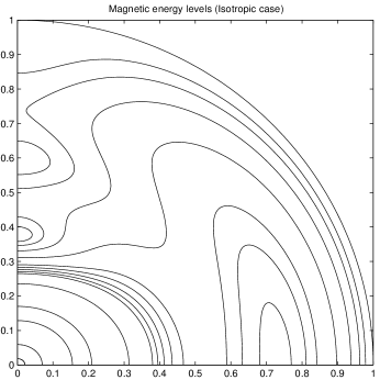
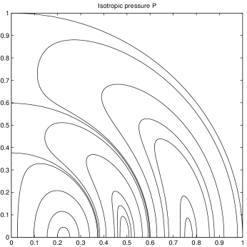
Figure 1: Constant levels of magnetic energy density (left) and pressure (right) in the static isotropic MHD equilibrium (Bobnev’s solution (29,30)) for $R=1,\lambda_{=}\lambda_{3}\approx 6.161$. $z$ (upward) is the symmetry axis, $x$ (horizontal) is the radial axis.

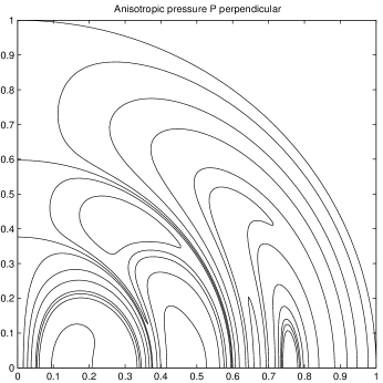
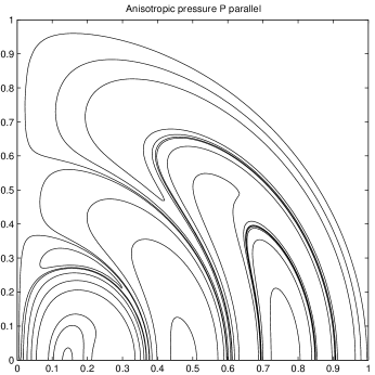
Figure 2: Surfaces of constant level of plasma pressure components $P,~{}p_{\perp}~{},p_{\parallel}$ in an anisotropic vortex.

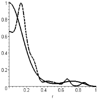
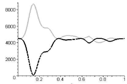
Figure 3: Left: Comparison of energy densities ${\bf{B}}_{v}^{2}/2$ and ${\bf{B}}_{1}^{2}/2$ for isotropic and anisotropic plasma vortex in the radial direction. Right: Comparison of plasma pressure components $P,~{}p_{\perp}~{},p_{\parallel}$ in an anisotropic vortex in the radial direction.

Similarly to the isotropic vortex, the anisotropic solution has the boundary condition ${\bf B}|_{\rho=R}=0,$ and ${\bf B}|_{\rho=0}=B_{0}{\bf e}_{z}$ at the origin. The magnetic field is chosen to be zero outside the plasma domain.

As seen from Fig. 3 (right) and expressions (14),(18), plasma pressure components $p_{\parallel 1},p_{\perp 1}$ of the anisotropic vortex are different within the plasma domain $r<1$, but equal on the boundary. Thus the presented solution describes a localized anisotropic plasma formation confined by external gas pressure. (We note that both known vortex-like isotropic solutions, by Bobnev [10] and by Kaiser and Lortz [35] have the same feature: the plasma ball is confined by outer gas pressure.)

5 Further remarks

1. The Lie symmetry-based approach remains to be one of the most generally applicable and successful coordinate-independent techniques for generating exact solutions and reduced (invariant) versions of nonlinear partial differential equations for obtaining self-similar solutions. For an ODE, knowledge of Lie symmetries always leads to the reduction of order of the equation under consideration, by the number up to the dimension of the symmetry group [14]. The global form of Lie point symmetries is used to generate several-parameter (in some important cases, infinite-parameter) families of exact solutions from known ones.

In this paper we have presented an example when the complete straightforward Lie analysis reveals an infinite-dimensional symmetry group for static anisotropic (Chew-Goldberger-Low) Plasma Equilibrium equations. The existence of this symmetry Lie group leads to a dramatic extension of the set of known solutions, bringing in physically relevant anisotropic static plasma configurations related to solutions of static MHD equations. In particular, one may construct new static CGL equilibria in axial and helical symmetry using corresponding Grad-Shafranov and JFKO equations (Section 4.1), or from known static MHD configurations (as illustrated by the example in Section 4.2).

2. The potential symmetry theory [14] and the algorithmic framework for nonlocally-related potential systems and subsystems [15] has been demonstrated to be useful for calculating new nonlocal symmetries and new nonlocal conservation laws for a given system of PDEs, especially in the case of two independent variables. However in a PDE system with $n\geq 3$ independent variables, such as MHD or CGL systems discussed in this paper, the corresponding potential system is underdetermined, and requires suitable gauge constraints (in the form of additional equations on the potential variables) to be imposed in order to find nonlocal symmetries [38]. The question of choosing gauge constraints that lead to potential symmetries is yet to be answered. Future work will concentrate on this problem, in particular, for the system of static MHD equations, which can be totally written as a set of four conservation laws [36].

3. Systems of static MHD (1) and CGL (2)-(4) equations are examples of systems where the use of appropriate analytical computation software is helpful for the full point symmetry analysis and leads to finding new symmetry structure (Section 3.) In the same manner, infinite symmetries for dynamic MHD [18] and CGL [20] equilibrium equations can be found within Lie group analysis framework [16, 17], but have been overlooked due to incomplete analysis in the preceding literature (e.g. [37]).

The routines of GeM package for Maple presented and used in this work (and in parts in [18, 17]) perform local (Lie, contact, Lie-Bäcklund) and nonlocal symmetry and conservation law analysis of ordinary and partial differential equations automatically, i.e. without human intervention. Corresponding determining systems are automatically generated and reduced, and in most cases completely solved. The package routines allow the solution of important symmetry/conservation law classification problems for systems with arbitrary constitutive functions. To the best of the author’s knowledge, GeM is the most complete and fast end-user-oriented package for Maple.

Further development of the GeM package that will include routines for explicit reconstruction of conservation law fluxes and densities and automatic construction of trees of nonlocally-related potential systems and subsystems [15] is one of the directions of current work.

4. Further research, jointly with G. Bluman and other collaborators, will include the complete symmetry and conservation law analysis of dynamic CGL and MHD systems, as well as the construction of trees of nonlocally-related potential systems and subsystems and search for nonlocal symmetries and conservation laws of Nonlinear Telegraph (NLT) equations and equations of gas/fluid dynamics (which is partly complete).

Acknowledgements

The author is grateful to George Bluman and Oleg I. Bogoyavlenskij for the discussion of results.

———————————–

Appendix A ”GeM” Symmetry computation module: a brief routine description

Here we outline the program for group analysis of static MHD equations (1) using the GeM package.

First, dependent and independent variables, free functions and free constants are declared. For example, for the CGL static equilibrium system (2), the statement is

$$\verb"acgen_decl_vars([x,y,z], [B1(x,y,z),B2(x,y,z),B3(x,y,z),P(x,y,z)],[],[],0);"$$

Here $B1,B2,B3$ are three components of the magnetic field vector $\bf B$; the empty bracket pairs $[~{}]$ indicate that no arbitrary functions and constants are present; $0$ stands for the highest order of derivative on which arbitrary functions depend.

Then equations are declared by calling the routine

$$.\begin{array}[]{ll}\verb"acgen_decl_eqs( "\\ \verb"[ equ[1], equ[2], equ[3], equ[4] ], "\\ \verb"1,"\\ \verb"[diff(B1(x,y,z),x), diff(P(x,y,z),x), diff(P(x,y,z),y), diff(P(x,y,z),z)]"\\ \verb");"\\ \end{array}$$

where equ[1], …,equ[4] are properly prepared Maple expressions for static MHD equations (1).

Within this routine, all derivatives are defined as symbols: $\partial B_{1}/\partial x\equiv\verb"B1x"$, etc. For example, the Maple expression for the equation ${\rm{div}}~{}{\bf{B}}=0$

$${\frac{\partial}{\partial x}}{\it B1}\left(x,y,z\right)+{\frac{\partial}{\partial y}}{\it B2}\left(x,y,z\right)+{\frac{\partial}{\partial z}}{\it B3}\left(x,y,z\right)=0$$

is represented as

$$\verb"B1x + B2y + B3z = 0".$$

After this conversion, the unknown tangent vector field components $\xi^{i},\eta^{k}$ are not composite functions but functions of all ”independent variables”, which include dependent and independent variables of the system under consideration and all partial derivatives.

The variables on which tangent vector field components $\xi^{i},\eta^{k}$ depend are specified by using

$$\verb"acgen_def_vf([B1(x,y,z),B2(x,y,z),B3(x,y,z),T(x,y,z),P(x,y,z)],0,0);"$$

The function names of resulting tangent vector field components are stored in a set V_F_COORDS_.

The overdetermined system of determining equations system variables on which depend are determined by using

$$\verb"acgen_get_split_sys();"$$

(which generates 133 equations) and reduced by

$$\verb"rss:=rifsimp(sys_l2,convert(V_F_COORDS_,list));"$$

to obtain 49 simple equations found in the variable rss[Solved].

The final answer for tangent vector field components in this case is easily obtained by hand, or Maple built-in integrator

$$\verb"expand(pdsolve(rss[Solved]));"$$

and provides the results listed in the formulation of Theorem 1.

We remark again that the built-in Maple routine ”pdsolve” for PDE integration sometimes produces incomplete answers and therefore is recommended only for preliminary analysis; the completeness of its output is to be verified by hand in every case.

Appendix B Proof of Theorem 2.

Proof of Theorem 2.

First we prove the formula (15). Using the vector calculus identity

$$\mathop{\hbox{\rm curl}}(a{\bf s})=a\mathop{\hbox{\rm curl}}({\bf s})+(\mathop{\hbox{\rm grad}}a)\times{\bf s}$$

and the formilas ${\bf{B}}\cdot\mathop{\hbox{\rm grad}}\tau=0$ and (2), one gets

$$\mathop{\hbox{\rm curl}}\left(\sqrt{1-\tau}{\bf{B}}\right)\times\left(\sqrt{1-\tau}{\bf{B}}\right)=(1-\tau)\mathop{\hbox{\rm curl}}{\bf{B}}\times{\bf{B}}-\frac{1}{2}\frac{\sqrt{1-\tau}}{\sqrt{1-\tau}}(\mathop{\hbox{\rm grad}}\tau\times{\bf{B}})\times{\bf{B}}$$

$$={\rm{grad}}~{}p_{\perp}+\tau~{}{\rm{grad}}\frac{{{\bf{B}}^{2}}}{2}+\frac{{\bf{B}}^{2}}{2}\mathop{\hbox{\rm grad}}\tau=\mathop{\hbox{\rm grad}}\left(p_{\perp}+\tau\frac{{{\bf{B}}^{2}}}{2}\right).$$

We thus observe that the quantity $p_{\perp}+\tau\frac{{\bf{B}}^{2}}{2}$ is constant on magnetic field lines: $\mathop{\hbox{\rm grad}}\left(p_{\perp}+\tau\frac{{{\bf{B}}^{2}}}{2}\right)\perp{\bf{B}}$. The same is true for $\tau$. Hence without loss of generality

$$F\left(\tau,p_{\perp}+\tau\frac{{\bf{B}}^{2}}{2}\right)=F(\Psi),$$

where $\Psi$ is a function constant on magnetic field lines.

We may also check that the quantity $p_{\perp}+\tau\frac{{\bf{B}}^{2}}{2}$ is invariant under the action of $X_{\infty}$:

$$\frac{\partial}{\partial\varepsilon}\left(p_{\perp}+\tau\frac{{\bf{B}}^{2}}{2}\right)^{\prime}|_{\varepsilon=0}=\frac{\partial}{\partial\varepsilon}p^{\prime}_{\perp}|_{\varepsilon=0}+\frac{{\bf{B}}^{2}}{2}\frac{\partial}{\partial\varepsilon}\tau^{\prime}|_{\varepsilon=0}+\tau\frac{\partial}{\partial\varepsilon}\frac{{{\bf{B}^{\prime}}^{2}}}{2}|_{\varepsilon=0}=0;$$

hence $\Psi$ may be chosen so that it is also invariant under the action of $X_{\infty}$.

This allows the integration of Lie equations (9), and the global group of transformations is

$$B_{k,1}=B_{k}\exp\left(aF\left(\Psi\right)\right),~{}~{}(1-\tau_{1})=(1-\tau)\exp\left(-2\varepsilon F\left(\Psi\right)\right),$$

$$p_{\perp 1}=p_{\perp}+\frac{{\bf{B}}^{2}}{2}\left(1-\exp\left(-2\varepsilon F\left(\Psi\right)\right)\right),$$

In (13),(14), $M$ is a sufficiently smooth function separated from zero. It is connected with F as follows. The case $M\geq 0$ is obtained by assigning

$$M(\Psi):=\exp\left(\varepsilon F\left(\Psi\right)\right),$$

where F is an arbitrary smooth real-valued function; the case $M<0$ - the same way by taking

$$F\left(\Psi\right)=\frac{i\pi}{\varepsilon}+G\left(\Psi\right),$$

where $G$ is an arbitrary smooth real-valued function.

This completes the proof of Theorem 2.$\blacksquare$

References

- [1] Tanenbaum B. S. Plasma Physics. McGraw-Hill, (1967).
- [2] Chew G.F, Goldberger M.L., Low F.E., Proc. Roy. Soc. 236(A), 112 (1956).
- [3] Biskamp D. Nonlinear Magnetohydrodynamics. Cambridge Univ. Press (1993).
- [4] Grad H., Rubin H., in the Proceedings of the Second United Nations International Conference on the Peaceful Uses of Atomic Energy, 31, United Nations, Geneva, 190 (1958).
- [5] Shafranov. V. D.. JETP 6, 545 (1958).
- [6] Johnson J. L., Oberman C. R., Kruskal R. M., and Frieman E. A. Phys. Fluids 1, 281 (1958).
- [7] Bogoyavlenskij O. I. Phys. Rev. Lett. 84, 1914 (2000).
- [8] Kadomtsev B. B. JETP 10, 962 (1960).
- [9] Kaiser R. and Lortz D. Phys. Rev. E 52(3), 3034 (1995).
- [10] Bobnev A. A. , Magnitnaya Gidrodinamika 24(4), 10 (1998).
- [11] Bogoyavlenskij O. I. , Phys. Rev. E 62(6), 8616 (2002).
- [12] Cheviakov A. F. Phys. Rev. Lett. 94, 165001 (2005).
- [13] Olver P. J. Applications of Lie groups to differential equations. New York: Springer-Verlag (1993).
- [14] Bluman G.W., Kumei S. Symmetries and Differential Equations, Springer-Verlag (1989).
- [15] Bluman G., Cheviakov A. F. ”Framework for potential systems and nonlocal symmetries: Algorithmic approach”. Submitted to Journal of Mathematical Physics. (2005).
- [16] Cheviakov A. F. Phys. Lett. A. 321/1, 34-49 (2004).
- [17] A. F. Cheviakov, in Proc. of ”Symmetry in Nonlinear Mathematical Physics - 2003” International Conf., NAS Ukraine, Kiev , Vol. 50, Part 1, 69 (2004).
- [18] Bogoyavlenskij O. I. Phys. Lett. A. 291 (4-5), 256-264 (2001).
- [19] Bogoyavlenskij O. I. Phys. Rev. E. 66 (5), #056410 (2002).
- [20] Cheviakov A.F. and Bogoyavlenskij O.I., J. Phys. A 37, 7593 (2004).
- [21] Mansfield E.L. Differential Groebner Bases. Ph.D. diss., University of Sydney (1991)
- [22] Ollivier F. Standard Bases of Differential Ideals. Lecture Notes in Comp. Sci. 508, 304-321 (1991).
- [23] Reid G.J., Wittkopf A.D., and Boulton A. Eur. J. Appl. Math. 7, 604-635 (1996).
- [24] Reid G.J., Wittkopf A.D. Proc. ISSAC 2000. 272-280, ACM Press (2000).
- [25] Boulier F., Lazard D., Ollivier F. and Petitot M. Proc. ISAAC’95. ACM Press (1995).
- [26] Hubert E. J. Symb. Comput. 29, 641-662 (2000).
- [27] Hereman W. Mathematical and Computer Modelling , vol. 25, pp. 115-132 (1997).
- [28] Wolf T., ”Crack, LiePDE, ApplySym and ConLaw, section 4.3.5 and computer program on CD-ROM” in: Grabmeier, J., Kaltofen, E. and Weispfenning, V. (Eds.): Computer Algebra Handbook, Springer pp. 465-468 (2002).
- [29] The package, a brief description and examples are available for download at http://www.math.ubc.ca/ alexch/GEM.htm.
- [30] Beskin V. S. and Kuznetsova I. V., Astroph. J. 541, 257 (2000).
- [31] Erkaev N.V. et al, Adv. Space Res. 28(6), 873 (2001).
- [32] Kruskal M.D., Kulsrud R.M. Phys. Fluids. 1, 265 (1958).
-
[33]
The packages for Maple such as
Rif(the extended version of the ”Standard Form” package by Reid and Wittkopf anddiffgrob2are frequently used for the purpose of reduction of large PDE systems. - [34] Clemmow, P. C., Dougherty, J. P. Electrodynamics of Particles and Plasmas (Reading: Addison-Wesley), 385 (1969).
- [35] Kaiser R., Lortz D. Phys. Rev. E 52 (3), 3034 (1995).
- [36] Cheviakov A.F.: Ph.D. thesis. Queen’s University, Kingston, Canada (2004).
- [37] CRC handbook of Lie group analysis of differential equations. (Editor: N.H. Ibragimov). Boca Raton, Fl.: CRC Press (1993).
- [38] Anco, S. and Bluman, G., ”Nonlocal symmetries and conservation laws of Maxwell’s equations.” J. Math. Phys. 38, 3508-3532 (1997).