DESY 05-185
SFB/CPP-05-60
August 2005
Symbolic Summation and Higher Orders in Perturbation Theory

Abstract

Higher orders in perturbation theory require the calculation of Feynman integrals at multiple loops. We report on an approach to systematically solve Feynman integrals by means of symbolic summation and discuss the underlying algorithms. Examples such as the non-planar vertex at two loops, or integrals from the recent calculation of the three-loop QCD corrections to structure functions in deep-inelastic scattering are given.

1 INTRODUCTION

Symbolic summation amounts to finding a closed-form expression for a given sum or series. Systematic studies have been pioneered by Euler [1], and for specific sums, exact formulae have been known for a long time. Today, general classes of sums, for example harmonic sums, have been investigated (see e.g. Refs. [2]) and symbolic summation has further advanced through the development of algorithms suitable for computer algebra systems. Here, the possibility to obtain exact solutions by means of recursive methods has lead to significant progress, for instance in the summation of rational or hypergeometric series, see e.g. Ref. [3].

In quantum field theory, higher-order corrections in perturbation theory require the evaluation of Feynman diagrams, which describe real and virtual particles in a given scattering process. In mathematical terms, Feynman diagrams are given as integrals over the loop momenta of the associated particle propagators. These integrals may depend on multiple scales and are usually divergent, thus requiring some regularization. The standard choice is dimensional regularization, i.e. an analytical continuation of the dimensions of space-time from 4 to $D$, which keeps underlying gauge symmetries manifest. Analytical expressions for Feynman integrals in $D$ dimensions may lead to transcendental or generalized hypergeometric functions, which have a series representation through nested sums with symbolic arguments. The main computational task is then to obtain the Laurent series upon expansion of the relevant functions in the small parameter $\epsilon=(D-4)/2$.

2 ALGORITHMS

The basic recursive definition of nested sums is given by [4]

$$S(n;m_{1},...,m_{k};x_{1},...,x_{k})=$$ (1)

$$\sum\limits_{j=1}^{n}{x_{1}^{j}\over j^{m_{1}}}S(j;m_{2},...,m_{k};x_{2},...,x_{k})\,.$$

where generally all $|x_{i}|\leq 1$. The sum of all $m_{i}$ is called the weight of the sum, while the index $k$ denotes the depth. This definition actually includes as special cases the classical polylogarithms, Nielsen functions, multiple and harmonic polylogarithms [5, 6, 7] in their series representations. For all $x_{i}=1$, the above definition reduces to harmonic sums [1, 8, 9, 10] and, if additionally the upper summation boundary $n\to\infty$, one recovers the (multiple) zeta values associated to Riemann’s zeta-function [2].

As an important property the $S$-sums in Eq. (1) obey the well-known algebra of multiplication. Specifically, any product

$$S(n;m_{1},...,m_{k};x_{1},...,x_{k})$$ (2)

$$\times S(n;m^{\prime}_{1},...,m^{\prime}_{l};x^{\prime}_{1},...,x^{\prime}_{l})\,,$$

can be expressed again as a sum of single nested sums, hence in a canonical form, which is an important feature for practical applications. The underlying algebraic structure in Eq. (2) is a Hopf algebra, being realized as a quasi-shuffle algebra here, see e.g. Refs. [4, 11, 12, 13] . The algorithm can be implemented very efficiently on a computer, see e.g. Refs. [10, 14].

For the manipulation of the $S$-sums, we classify certain types of transcendental sums. All sums in these classes can be solved recursively, i.e. they can be expressed in canonical form. The underlying algorithms realize a creative telescoping. They either reduce successively the depth or the weight of the inner sum, so that eventually the inner nestings vanish. Finally, the results can be written in the basis of Eq. (1), (as $S$-sums with upper summation limit $n$) or as multiple polylogarithms (which are $S$-sums to infinity).

Besides the quasi-shuffle algebra of multiplication in Eq. (2), the procedure relies on algebraic manipulations, such as partial fractioning of denominators, shifts of the summation ranges and synchronization of summation boundaries of the individual sums.

Specifically, we consider convolutions,

$$\sum\limits_{j=1}^{n-1}{x_{1}^{j}\over j^{m_{1}}}S(j;m_{2},...,m_{k};x_{2},...,x_{k})$$

$$\times{(x^{\prime}_{1})^{n-j}\over(n-j)^{m^{\prime}_{1}}}S(n-j;m^{\prime}_{2},...,m^{\prime}_{l};x^{\prime}_{2},...,x^{\prime}_{l})\,,$$

conjugations,

$$-\sum\limits_{j=1}^{n}\,\left(\begin{array}[]{c}n\\ j\end{array}\right)\,(-1)^{j}$$ (7)

$$\times{x_{1}^{j}\over j^{m_{1}}}S(j;m_{2},...,m_{k};x_{2},...,x_{k})\,,\,\,$$

and binomial convolutions,

$$-\sum\limits_{j=1}^{n-1}\,\left(\begin{array}[]{c}n\\ j\end{array}\right)\,(-1)^{j}$$

$$\times{x_{1}^{j}\over j^{m_{1}}}S(j;m_{2},...,m_{k};x_{2},...,x_{k})$$

$$\times{(x^{\prime}_{1})^{n-j}\over(n-j)^{m^{\prime}_{1}}}S(n-j;m^{\prime}_{2},...,m^{\prime}_{l};x^{\prime}_{2},...,x^{\prime}_{l})\,.\,\,$$

In all cases, the upper summation boundary should be consistent with the defining range of the binomials and the $S$-sums.

3 APPLICATIONS

In perturbation theory, one way to classify Feynman integrals is according to the number of scales, i.e. the number of non-vanishing scalar products of external momenta or particle masses. According to this criterion, analytical expressions in $D$ dimensions for the Laurent series in $\epsilon$ either lead to transcendental numbers like (multiple) zeta values or (multiple) polylogarithms. Other classification criteria are, of course, the topology of a Feynman integral (number of loops and external legs).

3.1 One-scale problems

Prominent examples of one-scale problems are massless two-point functions [15, 16, 17]. In particular, the massless two-loop self-energy ${\rm T1}$ has not only been of practical importance from a phenomenological perspective, but received also quite some interest from number theorists. For arbitrary powers of propgators, it is given by

$${\rm T1}(\nu_{1},\nu_{2},\nu_{3},\nu_{4},\nu_{5})\,=\,\int\frac{{\hbox{d}}^{D}p_{1}}{(2\pi)^{D}}\,\int\frac{{\hbox{d}}^{D}p_{2}}{(2\pi)^{D}}$$ (12)

$$\times\,{1\over\left(p_{1}^{2}\right)^{\nu_{1}}\left(p_{2}^{2}\right)^{\nu_{2}}\left(p_{3}^{2}\right)^{\nu_{3}}\left(p_{4}^{2}\right)^{\nu_{4}}\left(p_{5}^{2}\right)^{\nu_{5}}},$$

where $p_{3}=p_{2}-q$, $p_{4}=p_{1}-q$, $p_{5}=p_{1}-p_{2}$. Graphically, it is displayed in Fig. 1.

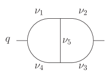
Figure 1: The two-loop self-energy ${\rm T1}$.

Here the interesting question has been which types of (transcendental) numbers appear in the $\epsilon$-expansion of this integral. For powers of the propagators of the form $\nu_{i}=1+\epsilon$, $i=1,\dots,5$ it was known from explicit calculations up to the $\epsilon^{9}$-term (heavily relying on symmetry properties) that multiple zeta values occur [15]. However, it was unclear whether this suffices to all orders in $\epsilon$. Eventually, by deriving a double sum of (generalized) hypergeometric type, it was proven that multiple zeta values are indeed sufficient [16].

Currently, with the help of symbolic summation the $\epsilon$-expansion is known to the $\epsilon^{13}$-term [18]. The depth is limited by the fact that harmonic sums in infinity are expressed in a basis of transcendental numbers only up to weight 16.

Another example for a one-scale problem, that received attention recently [19, 20] is the non-planar vertex at two loops, which enters in calculations of the quark and gluon form factors [19, 21] in QCD. Here the basic integral (displayed in Fig. 2) is given by

$$V_{\rm NO}(\nu_{1},\nu_{2},\nu_{5},\nu_{6},\nu_{7},\nu_{8})\,=\,\int\frac{{\hbox{d}}^{D}p_{1}}{(2\pi)^{D}}\,\int\frac{{\hbox{d}}^{D}p_{2}}{(2\pi)^{D}}$$ (13)

$$\times\,{1\over\left(p_{1}^{2}\right)^{\nu_{1}}\left(p_{2}^{2}\right)^{\nu_{2}}\left(p_{5}^{2}\right)^{\nu_{5}}\left(p_{6}^{2}\right)^{\nu_{6}}\left(p_{7}^{2}\right)^{\nu_{7}}\left(p_{8}^{2}\right)^{\nu_{8}}},$$

where $p_{5}=p_{4}-p_{7}$, $p_{6}=p_{1}-q$, $p_{7}=p_{2}-p_{1}$, $p_{8}=p_{2}-p_{3}$ and $q^{2}=(p_{3}-p_{4})^{2}$.

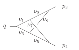
Figure 2: The non-planar two-loop vertex $V_{\rm NO}$.

For general powers of propagators, $V_{\rm NO}$ can be written as a double sum over Gamma functions, and if all $\nu_{i}=1$, an expression in terms of hypergeometric functions ${}_{3}F_{2}$ and ${}_{4}F_{3}$ has been given in Ref. [20]. After expansion, the sum can be solved in terms of the Riemann zeta function to any order in $\epsilon$ using the algorithms for harmonic sums [10, 14] coded, as all our symbolic manipulations, in Form [22]. We find the following expansion to order $\epsilon^{5}$,

$$V_{\rm NO}(1,1,1,1,1,1)\,=\,$$ (14)

$$S_{\Gamma}^{2}\,\left(-q^{2}\right)^{-2-2\epsilon}\,\Bigg{[}-{1\over\epsilon^{4}}+{5\*{\zeta_{2}}\over\epsilon^{2}}+{27\*{\zeta_{3}}\over\epsilon}$$

$$+23\*{\zeta_{2}}^{2}-\epsilon\*(48\*{\zeta_{2}}\*{\zeta_{3}}-117\*{\zeta_{5}})+\epsilon^{2}\*\bigl{(}{456\over 35}\*{\zeta_{2}}^{3}$$

$$-267\*{\zeta_{3}}^{2}\bigr{)}-\epsilon^{3}\*\bigl{(}{1962\over 5}\*{\zeta_{2}}^{2}\*{\zeta_{3}}+240\*{\zeta_{2}}\*{\zeta_{5}}+6\*{\zeta_{7}}\bigr{)}$$

$$-\epsilon^{4}\*\bigl{(}{3219\over 7}\*{\zeta_{2}}^{4}-264\*{\zeta_{2}}\*{\zeta_{3}}^{2}+2466\*{\zeta_{3}}\*{\zeta_{5}}$$

$$-264\*{\zeta_{5,3}}\bigr{)}-\epsilon^{5}\*\bigl{(}{2832\over 5}\*{\zeta_{2}}^{3}\*{\zeta_{3}}+2718\*{\zeta_{2}}^{2}\*{\zeta_{5}}$$

$$+1218\*{\zeta_{2}}\*{\zeta_{7}}+1626\*{\zeta_{3}}^{3}+{20777\over 3}\*{\zeta_{9}}\bigr{)}\Bigg{]}\,,$$

where we have taken out the usual ${\overline{\mbox{MS}}}$-scheme factor

$$S_{\Gamma}={(4\pi)^{-2+\epsilon}\over\Gamma(1-\epsilon)}\,.$$ (15)

This completes the section of examples with one-scale.

3.2 Two-scale problems

Nice examples of two-scale problems are provided by the recent calculation of the three loop corrections in Quantum Chromodynamics (QCD) to the structure functions of deep-inelastic scattering [23, 24, 25]. Here, the two scales are the virtuality of the exchanged gauge boson $Q^{2}=-q^{2}$ and the scalar product of the boson’s and nucleon’s momenta, $2p\cdot q$, both combining to Bjorken’s dimensionless variable $x=Q^{2}/(2p\cdot q)$.

The Feynman integrals under consideration can be expressed in nested sums and solved with the help of symbolic summation as follows. Imagine a mapping of a given integral $I(x)$ depending on $x$, $0\leq x\leq 1$ to the space of discrete variables $I(N)$, $N\in{\mathbf{N}}$, which is accomplished by means of an integral transformation, e.g. a Mellin transformation. Then one can obtain difference equations for the Feynman integral $I(N)$, which may be written as [26]

$$a_{0}(N)\,I(N)+a_{1}(N)\,I(N-1)+\ldots$$ (16)

$$+a_{m}(N)\,I(N-m)\>=\>G(N)\,,$$

where $G(N)$ is some inhomogeneous term and $a_{i}$ are some coefficients depending on $N$ (and perhaps on $\epsilon$). The solution of Eq. (16) needs $m$ boundary conditions $I(0),\dots,I(m-1)$.

Single-step difference equations can be summed up analytically in closed form. Suppose we have the equation

$$a_{0}(N)\,I(N)-a_{1}(N)\,I(N-1)\>=\>G(N)\,,$$ (17)

then its solution will be

$$I(N)=\frac{\prod_{j=1}^{N}a_{1}(j)}{\prod_{j=1}^{N}a_{0}(j)}\,I(0)$$ (18)

$$+\sum_{i=1}^{N}\frac{\prod_{j=i+1}^{N}a_{1}(j)}{\prod_{j=i}^{N}a_{0}(j)}\,G(i)\,.$$

In the case that the functions $a_{i}$ can be factorized in linear polynomials of the type $N+m+n\,\epsilon$ with $m,n$ being integer and $N$ being symbolic, the products can be written as combinations of Gamma functions. In the presence of parametric dependence on $\epsilon$ the Gamma functions should be expanded around $\epsilon=0$, leading to factorials and harmonic sums. If the function $G(N)$ is expressed as a Laurent series in $\epsilon$ with the coefficients being combinations of harmonic sums in $N+m$ and powers of $N+m$, $m$ being a fixed integer, the sum in Eq. (18) can be done and $I(N)$ will be a combination of harmonic sums in $N+k$ and powers of $N+k$ with $k$ being a fixed integer.

Eq. (16) is an example of a recursion for Feynman integrals with dependence on symbolic parameters. Solutions such as Eq. (18) allow for an efficient implementation in computer algebra systems like Form [22] resulting in a largely automatic build-up of nested sums. For calculation of QCD corrections to structure functions mentioned above, a systematic evaluation of nested sums was required for all integrals occurring in approximately 10.000 Feynman diagrams. Because of the expressions being of excessive size at intermediate stages this task was well suited for the computer algebra system Form and the Summer package [10] for nested sums.

3.3 Multi-scale problems

Multi-scale problems arise in the calculation of cross sections with more kinematical invariants, like e.g. jet cross sections. The methods and algorithms for generalized sums have already been used in full-fledged QCD calculations, for instance in the evaluation of higher order corrections to $e^{+}e^{-}\to 3\mbox{jets}$ [27].

In general, Eqs. (2)–(2) may also be used to expand higher transcendental functions in a small parameter around integer values. Starting from the series representation of, e.g. the first Appell function

$$F_{1}(a,b_{1},b_{2};c;x_{1},x_{2})\,=\,$$ (19)

$$\sum\limits_{m_{1}=0}^{\infty}\sum\limits_{m_{2}=0}^{\infty}\frac{a^{\overline{m_{1}+m_{2}}}b_{1}^{\overline{m_{1}}}b_{2}^{\overline{m_{2}}}}{c^{\overline{m_{1}+m_{2}}}}\frac{x_{1}^{m_{1}}}{m_{1}!}\frac{x_{2}^{m_{2}}}{m_{2}!}\,,$$

or the second Appell function

$$F_{2}(a,b_{1},b_{2};c_{1},c_{2};x_{1},x_{2})\,=\,$$ (20)

$$\sum\limits_{m_{1}=0}^{\infty}\sum\limits_{m_{2}=0}^{\infty}\frac{a^{\overline{m_{1}+m_{2}}}b_{1}^{\overline{m_{1}}}b_{2}^{\overline{m_{2}}}}{c_{1}^{\overline{m_{1}}}c_{2}^{\overline{m_{2}}}}\frac{x_{1}^{m_{1}}}{m_{1}!}\frac{x_{2}^{m_{2}}}{m_{2}!}\,,$$

we see that Eqs. (2)–(2) apply if the expansion parameter $\epsilon$ occurs in the argument of the rising factorials (Pochhammer symbols), defined as

$$f^{\overline{m}} = f(x)f(x+1)\dots f(x+m-1)\,.$$ (21)

It should also be stressed at this point, that although the definition of the $S$-sums in Eq. (1) is very general, the specific algorithms for convolution, conjugation etc. are subject more restrictive assumptions.

In particular, the algorithms underlying the evaluation of Eqs. (2)–(2) do rely on the fact that the modulus of the summation index in the argument of the $S$-sums or in the denominators is always one. This changes, if for instance hypergeometric functions ${}_{J}F_{J-1}$ (or more generally Gamma-functions) are expanded around half-integer values. Such a situation occurs for example in the calculation of massive higher loop integrals in Bhabha scattering [28].

Some extensions of the summation algorithms for expansion around rational values, leading e.g. to binomial sums and inverse binomial sums are discussed in Ref. [29, 30].

4 CONCLUSION

Symbolic summation has advanced to an important method for the calculation of higher order corrections in perturbative quantum field theory. The field has seen significant progress during the past years and we have given various examples from complete calculations, e.g. the recent evaluation of the third-order contributions in perturbative QCD to the structure functions of deep-inelastic scattering [23, 24, 25]. These cutting edge calculations show that the method of symbolic summation provides very powerful means for the practical computations of Feynman diagrams.

In closing, we note that all practical applications do heavily rely on computer algebra implementations of the algorithms discussed here. In the symbolic manipulation program Form [22], which is a fast and efficient computer algebra system to handle large expressions, harmonic sums can be manipulated with the Summer package [10]. For the $S$-sums of Eq. (1) there exists an extension, the XSummer package [14] in Form , which implements algorithms of Eqs. (2)–(2). As an alternative within the GiNaC framework [31] the package nestedsums [32] provides similar functionalities. Very recently, also Ref. [33] appeared, which limits itself to the problem of expanding hypergeometric functions ${}_{J}F_{J-1}$ around integer parameters to arbitrary order and provides an implementation in Mathematica .

We believe all these packages may also be useful for a larger community.

References

- [1] L. Euler, Novi Comm. Acad. Sci. Petropol. 20 (1775) 140
-
[2]
M.E. Hoffman, http://www.usna.edu
/Users/math/meh/biblio.html -
[3]
M. Petkovsek, H. Wilf and
D. Zeilberger,
http://www.cis.upenn.edu/~wilf/AeqB.html - [4] S. Moch, P. Uwer and S. Weinzierl, J. Math. Phys. 43 (2002) 3363, hep-ph/0110083
- [5] A.B. Goncharov, Math. Res. Lett. 5 (1998) 497, (available at http://www.math.uiuc.edu/K-theory/0297)
- [6] J.M. Borwein et al., math.CA/9910045
- [7] E. Remiddi and J.A.M. Vermaseren, Int. J. Mod. Phys. A15 (2000) 725, hep-ph/9905237
- [8] D. Zagier, First Eur. Congr. of Math., Vol. II, Birkhäuser, Boston (1994) 497.
- [9] J.M. Borwein, D.M. Bradley and D.J. Broadhurst, (1996), hep-th/9611004
- [10] J.A.M. Vermaseren, Int. J. Mod. Phys. A14 (1999) 2037, hep-ph/9806280
- [11] M.E. Hoffman, J. Algebraic Combin. 11 (2000) 49, math.QA/9907173
- [12] S. Weinzierl, Eur. Phys. J. C33 (2004) s871, hep-th/0310124
- [13] J. Blümlein, Comput. Phys. Commun. 159 (2004) 19, hep-ph/0311046
- [14] S. Moch and P. Uwer, (2005), math-ph/0508008
- [15] D.J. Broadhurst, Nucl. Phys. Proc. Suppl. 116 (2003) 432, hep-ph/0211194
- [16] I. Bierenbaum and S. Weinzierl, Eur. Phys. J. C32 (2003) 67, hep-ph/0308311
- [17] S. Bekavac, (2005), hep-ph/0505174
-
[18]
J. Vermaseren, http://www.nikhef.nl/~form
/FORMdistribution/packages/summer - [19] S. Moch, J.A.M. Vermaseren and A. Vogt, JHEP 0508 (2005) 049, hep-ph/0507039
- [20] T. Gehrmann, T. Huber and D. Maitre, (2005), hep-ph/0507061
- [21] S. Moch, J.A.M. Vermaseren and A. Vogt, (2005), hep-ph/0508055
- [22] J.A.M. Vermaseren, (2000), math-ph/0010025
- [23] S. Moch, J.A.M. Vermaseren and A. Vogt, Nucl. Phys. B688 (2004) 101, hep-ph/0403192
- [24] A. Vogt, S. Moch and J.A.M. Vermaseren, Nucl. Phys. B691 (2004) 129, hep-ph/0404111
- [25] J.A.M. Vermaseren, A. Vogt and S. Moch, (2005), hep-ph/0504242
- [26] S. Moch and J.A.M. Vermaseren, Nucl. Phys. B573 (2000) 853, hep-ph/9912355
- [27] S. Moch, P. Uwer and S. Weinzierl, Phys. Rev. D66 (2002) 114001, hep-ph/0207043
- [28] M. Czakon, J. Gluza and T. Riemann, Phys. Rev. D 71 (2005) 073009, hep-ph/0412164
- [29] A.I. Davydychev and M.Y. Kalmykov, Nucl. Phys. B699 (2004) 3, hep-th/0303162
- [30] S. Weinzierl, J. Math. Phys. 45 (2004) 2656, hep-ph/0402131
- [31] C. Bauer, A. Frink and R. Kreckel, (2000), cs/0004015
- [32] S. Weinzierl, Comput. Phys. Commun. 145 (2002) 357, math-ph/0201011
- [33] T. Huber and D. Maitre, (2005), hep-ph/0507094