The scaling limit of two cluster boundaries in critical lattice models

Abstract

The probability that a point is to one side of a curve in Schramm-Loewner evolution ($\textrm{SLE}_{\kappa}$) can be obtained alternatively using boundary conformal field theory (BCFT). We extend the BCFT approach to treat two curves, forming, for example, the left and right boundaries of a cluster. This proves to correspond to a generalisation to SLE$(\kappa,\rho)$, with $\rho=2$. We derive the probabilities that a given point lies between two curves or to one side of both. We find analytic solutions for the cases $\kappa=0,2,4,8/3,8$. The result for $\kappa=6$ leads to predictions for the current distribution at the plateau transition in the semiclassical approximation to the quantum Hall effect.

1 Introduction

A large class of two-dimensional lattice models may be described in terms of a gas of non-intersecting loops. Examples include the boundaries of Ising spin clusters and percolation clusters, the boundaries of the clusters in the random cluster representation of the Potts model, the level lines of solid-on-solid models of the roughening transition, as well as dilute self-avoiding walks and polygons. These are in fact all special cases of the lattice O$(n)$ model.

The continuum limit of these curves is conjectured to be both scale and conformally invariant (a statement which may be made precise and which has been proved in a few cases.) A description of the whole ensemble of such curves is difficult, and instead it is simpler to focus initially on a single curve connecting two given points on the boundary of a simple connected domain, whose existence is guaranteed by the boundary conditions. The conformally invariant measure on such curves is conjectured to be given by Schramm(stochastic)-Loewner Evolution (SLE) [1] with parameter $\kappa$, where $n=-2\cos(4\pi/\kappa)$ with $2\leq\kappa\leq 8$. Many of the previously conjectured scaling dimensions of the O$(n)$ model, as well as other properties such as crossing formulae, have been derived using SLE [2, 3, 4]. The stochastic description naturally leads to second-order linear differential operators. Some of the scaling dimensions and correlation functions are given in terms of suitable eigenvalues and eigenfunctions of these.

An alternative description of the continuum limit of the critical O$(n)$ model is in terms of conformal field theory (CFT). This focusses on correlation functions of local scaling operators. Within CFT there is a correspondence between such operators and states in the radially quantised theory. These may be organised into irreducible representations of the Virasoro algebra satisfied by the generators $L_{n}$ of infinitesimal conformal transformations.

A connection between these two pictures was made in Refs. [5, 6]. As was conjectured in 1984[7], conditioning the CFT partition function on the existence of a curve starting at a given boundary point is equivalent to the insertion of a boundary operator $\phi_{2}$ which corresponds to a Virasoro representation with a level two null state: $L_{-2}|\phi_{2}\rangle=\alpha L_{-1}^{2}|\phi_{2}\rangle$. As was also shown in 1984[8], this implies that the correlators of this operator satisfy certain second-order linear differential equations. These are the same as those coming from SLE_κ, with the identification $\alpha=\kappa/4$.

However, CFT describes not only single curves but also many. Indeed the correlator

$$\langle\phi_{2}(x_{1})\phi_{2}(x_{2})\ldots\phi_{2}(x_{2N})\ldots\rangle$$ (1)

conditions the partition function on the existence of $N$ such non-intersecting curves, hitting the boundary at the points $\{x_{j}\}$. Such a correlation function satisfies $2N$ linear BPZ equations, one for each $x_{j}$. Note that the order in which they link up is not specified in the above. It may be made more precise by assigning O$(n)$ labels to the $\phi_{2}$s: only operators with the same label can then be connected by a curve. Alternatively, as we shall discuss further, the different ways the curves link up correspond to imposing different boundary conditions on the differential equations.

It is therefore straightforward in principle to derive within CFT many different results relating to how $N$ such curves cross a given domain. In practice, this becomes technically prohibitive. In this paper we consider the simplest non-trivial case with $N=2$. An interesting application of this for $\kappa=6$ (percolation) is the following problem, illustrated in Fig 1: consider critical site percolation in the upper half plane, and suppose that all the sites on the real axis are constrained to be white, except that at the origin, which is black. Moreover this site is conditioned to be connected to infinity by black sites, that is, it is part of an incipient infinite black cluster. The boundaries of this cluster then define two curves of the type we are considering.

Figure 1: An incipient infinite cluster containing a point on the boundary in critical site percolation on the triangular lattice. The scaling limit of the two curves forming its boundary is described by the results of this paper.

One of the simplest SLE results for a single curve, due to Schramm[9], gives the probability that a given point $\xi$ in the domain lies to the left (or right) of a single curve. While this had not in fact previously been discussed within CFT, its derivation from this point of view is straightforward[10]: the probability is given by the ratio of conditional expectation values

$$P(\xi)=\frac{\langle\Phi(\xi)\phi_{2}(x_{1})\phi_{2}(x_{2})\rangle}{\langle\phi_{2}(x_{1})\phi_{2}(x_{2})\rangle}\,,$$ (2)

where $\Phi(\xi)$ is the indicator function that the curve passes to the left(right) of $\xi$. [This behaves to all intents and purposes like a local operator with scaling dimension zero.] Specialising (without loss of generality, because of conformal invariance) to the case when the domain is the upper half plane and $x_{2}\to\infty$, the denominator becomes trivial and the numerator satisfies a BPZ equation with respect to $x_{1}$.

The generalisation of Eq. (2) to $N$ curves is straightforward. For example, for two curves in the upper half plane conditioned to connect $(x_{1},\infty)$ and $(x_{2},\infty)$

$$P(\xi)=\frac{\langle\Phi(\xi)\phi_{2}(x_{1})\phi_{2}(x_{2})\phi_{2}(\infty)\phi_{2}(\infty)\rangle}{\langle\phi_{2}(x_{1})\phi_{2}(x_{2})\phi_{2}(\infty)\phi_{2}(\infty)\rangle}\,,$$ (3)

where now $\Phi(\xi)$ is any of the indicator functions that $\xi$ lies to the left, or right, of both curves, or between them. Both numerator and denominator satisfy 2nd-order BPZ equations with respect to $x_{1}$ and $x_{2}$: the boundary conditions pick out which case is being computed.

These coupled partial differential equations are already too difficult to solve in closed form. However, they simplify in the limit when $\delta=x_{2}-x_{1}\ll|\xi|$, by a well-known property of CFT called the fusion rules. These state, roughly speaking, that in this limit the operator product $\phi_{2}(x_{1})\phi_{2}(x_{2})$ may be written

$$\phi_{2}(x_{1})\cdot\phi_{2}(x_{2})=\delta^{\alpha_{1}}\phi_{1}(x_{1})+\delta^{\alpha_{2}}\phi_{3}(x_{1})\,,$$ (4)

where the correlators of $\phi_{1}$ and $\phi_{3}$ satisfy respectively first and third order equations. In fact $\phi_{3}$ corresponds to a Virasoro representation with a null state at level 3. The null state condition may be computed explicitly, and hence the third-order equation. (This could also be obtained directly from the two 2nd order equations.) We also argue that if the curves are conditioned to go to infinity (rather than there being a single curve connecting $x_{1}$ and $x_{2}$) this picks out the second term in Eq. (4). The resulting correlation functions now depend only on $\arg(\xi-x_{1})$ and may be written as indefinite integrals of ordinary hypergeometric functions.

The layout of this paper is as follows. In the next section we recall the derivation of Schramm’s formula for a single curve using both SLE and CFT. Sec. 3 contains the main body of the CFT calculation for two curves. In Sec. 4 we present the results, in graphical form for $\kappa=6,8/3$. For some other values of $\kappa$ they may be expressed in terms of elementary functions. The limiting cases $\kappa=0$ and $\kappa=8$ are interesting.

In Sec. 5 we apply the results for $\kappa=6$ to the semi-classical limit of the quantum Hall plateau transition, where electrons in a strong magnetic field move in random scalar potential. If Coulomb interactions may be neglected, the guiding centres of the electrons approximately follow the level lines of the potential, which, in the scaling limit, are percolation cluster boundaries. At the critical point the half-plane geometry may be conformally transformed into a long strip, and our calculation gives information about the paths followed by the conduction electrons, and hence the mean current density across the strip.

Finally in Sec. 6 we discuss the equivalence between the BPZ equations of CFT and a postulated generalisation of SLE to multiple curves. The growth of a single curve, conditioned on the existence of the others, is described by a variant of SLE known as SLE$(\kappa,\rho)$ (with $\rho=2$), as asserted in several recent studies of multiple curves [11, 12, 13]. The CFT equations also suggest [14, 15] that it is possible to describe the joint measure on all the curves by a ‘multiple SLE’ in which they are grown simultaneously, as shown precisely in [12].

2 Schramm’s formula

In this section we review the computation of the probability that a given point $\xi$ lies to the left(right) of a single curve, from the points of view of both SLE and CFT.

2.1 CFT method

As discussed in Sec. 1, the probability is given as the ratio of correlators in Eq. (2). We take $x_{1}\to x$ and $x_{2}$ large (and eventually to infinity). Consider the effect of the infinitesimal conformal transformation $z\to z+\epsilon/(z-x)$, which is implemented by inserting into each correlator a factor

$$\int_{C}\frac{\epsilon\,T(z)}{z-x}\frac{dz}{2\pi i}\,,$$ (5)

where $C$ is a contour surrounding $x$ (but not $\xi$ or $x_{2}$), together with its reflection in the real axis. This may be evaluated in two ways: by shrinking the contour around $z=x$ and using the fact that the $O\big{(}(z-x)^{0}\big{)}$ term in the operator product expansion of $T(z)$ with $\phi_{2}(x)$ is (by definition) $L_{-2}\phi_{2}(x)=(\kappa/4)L_{-1}^{2}\phi_{2}(x)=(\kappa/4)\partial_{x}^{2}\phi_{2}(x)$; or by wrapping the contour around $\xi$ and $x_{2}$. The effect on $\Phi(\xi)$ is just to shift $\xi$, while the effect on $\phi_{2}(x_{2})$ is negligible as $x_{2}\to\infty$.

Equating these two ways of evaluating the insertion gives, as $x_{2}\to\infty$, the BPZ equation

$$\left(\frac{\kappa}{4}\frac{\partial^{2}}{\partial x^{2}}+2{\rm Re}\Big{[}\frac{1}{\xi-x}\frac{\partial}{\partial\xi}\Big{]}\right)P(\xi,x)=0\,,$$ (6)

where $P(\xi,x)$ is either probability. Since these only depend on the angle which $\xi-x$ makes with the axis, or equivalently the variable $t\equiv{\rm Re}(\xi-x)/{\rm Im}\xi$, this partial differential equation reduces to an ordinary one, of Riemann type. The boundary conditions are $P_{\rm left}\to 0$ as $t\to+\infty$ and $P_{\rm left}\to 1$ as $t\to-\infty$. The equation itself allows these two possible asymptotics – an explicit calculation determines the exponents as $|t|\to\infty$ to be $|t|^{-\gamma}$ with $\gamma=0$ or $\gamma=\tilde{x}_{2}=(8-\kappa)/\kappa$. The latter is the boundary 2-leg exponent: it arises as $t\to+\infty$ since the point $\xi$ traps the curve against the real axis so that, in effect, two mutually avoiding curves of the O$(n)$ model emerge from that point.

These boundary conditions then fix the solution to be

$$P_{\rm left}=\frac{1}{2}-\frac{\Gamma(\frac{4}{\kappa})}{\sqrt{\pi}\Gamma(\frac{8-\kappa}{2\kappa})}t\,_{2}F_{1}(\frac{1}{2},\frac{4}{\kappa};\frac{3}{2};-t^{2})\,.$$ (7)

Note that, because $P_{\rm left}+P_{\rm right}=1$ is a solution to the equation, any other, including Eq. (7), may be written as a quadrature of an elementary function.

2.2 SLE method

We summarise the theoretical physicist’s version[2, 5] of Schramm’s original argument. In SLE, the curve in the upper half plane from a point $a_{0}$ on the real axis to infinity is considered as being grown dynamically, introducing a fictitious time variable $t$ (obviously distinct from the variable $t$ defined above.) Let $K_{t}$ be the set consisting of the curve as grown up to time $t$ (as well as all points enclosed by the curve and between the curve and the real axis) so that the complement of this set in the upper half plane is simply connected. Let $g_{t}(z)$ be the (unique) conformal mapping of this complement to the whole upper half plane, normalised such that $g_{t}(z)=z+O(1/z)$ as $z\to\infty$. The coefficient of the $O(1/z)$ term is increasing with $t$, so ‘time’ can be reparametrised so this coefficient is exactly $2t$. The image of the growing tip of the curve under $g_{t}$ is a point $a_{t}$ on the real axis. Loewner showed that the time-evolution of $g_{t}$ satisfies

$$\frac{dg_{t}(z)}{dt}=\frac{2}{g_{t}(z)-a_{t}}\,.$$ (8)

Any suitably continuous function $a_{t}$ generates a curve. Schramm[1] showed that if this process is to generate a conformally invariant measure on curves, the only possibility is $a_{t}=\sqrt{\kappa}B_{t}+a_{0}$, with $B_{t}$ being a standard Brownian motion.

Now consider the problem at hand, with a curve $\gamma$ connecting $a_{0}$ to $\infty$, and a given point $\xi$ away from $a_{0}$. Evolve the SLE for an infinitesimal time $dt$. The function $g_{dt}$ will erase a short initial segment, and map the remainder of $\gamma$ into its image $\gamma^{\prime}$, which, however, by conformal invariance, will have the same measure as SLE started from $a_{dt}=a_{0}+\sqrt{\kappa}dB_{t}$. At the same time, $\xi\to\xi^{\prime}=\xi+2dt/(\xi-a_{0})$. Moreover, $\gamma^{\prime}$ lies to the left(right) of $\xi^{\prime}$ iff $\gamma$ lies to the left(right) of $\xi$. Therefore

$$P\big{(}\xi;a_{0}\big{)}=\langle P\big{(}\xi+2dt/(\xi-a_{0}),a_{0}+\sqrt{\kappa}dB_{t}\big{)}\rangle\,,$$ (9)

where the average $\langle\ldots\rangle$ is over all realisations of Brownian motion $dB_{t}$ up to time $dt$. Taylor expanding, using $\langle dB_{t}\rangle=0$ and $\langle(dB_{t})^{2}\rangle=dt$, and equating the coefficient of $dt$ to zero then gives exactly the CFT Eq. (6) if we set $a_{0}\to x$.

3 The differential equation for two curves

According to CFT the probability that a given point $\xi$ lies to the left, between or to the right of two curves starting at points $x_{1},x_{2}$ on the real axis is given by a ratio of correlators as in Eq. (3). The numerator and denominator each satisfy BPZ equations with respect to both $x_{1}$ and $x_{2}$. For general values, these are discussed further in Sec. 6. However, explicit analytic progress is only feasible in the limit when $\delta=x_{2}-x_{1}\to 0$, and we now treat this using established properties of CFT.

The operator product expansion of two $\phi_{2}$ operators is constrained by the fusion rules to have the form in Eq. (4). This means that every solution of the coupled second order BPZ equations may be written in this limit as a linear combination of functions $\delta^{\alpha_{j}}F_{j}(\xi,x,\delta)$, with $j=1,3$ and $x=(x_{1}+x_{2})/2$, and the functions $F_{j}$ having a regular power series expansion in $\delta$. The values of the $\alpha_{j}$ are determined by the differential equations to be $\alpha_{1}=-2h_{2}=-(6-\kappa)/\kappa$ and $\alpha_{3}=h_{3}-2h_{2}=2/\kappa$.

In general, the dominant behaviour as $\delta\to 0$ is given by $\alpha_{1}$, corresponding to the first term $\phi_{1}$ in the OPE, Eq. (4). This is just the identity operator, and it is straightforward to see that the corresponding solution $F_{1}$ is in fact a constant. The physical interpretation of this is that $x_{1},x_{2}$ are overwhelming likely to be the end-points of the same curve as $\delta\to 0$, which makes a very small excursion into the upper half plane. It has no effect on conditional probabilities of events further away. In order to condition the two curves each to go to infinity, we must therefore impose the condition that this term is absent in the solution.

This leaves the term in the OPE coupling to the $\phi_{3}$ operator. The leading behaviour of the probability function, Eq. (3), in this limit is therefore given by the ratio

$$P=\lim_{y\rightarrow\infty,\,x\rightarrow 0}\frac{\langle\Phi(\xi)\phi_{3}(x)\phi_{3}(y)\rangle}{\langle\phi_{3}(x)\phi_{3}(y)\rangle}\,.$$ (10)

In the limit $y\to\infty$ the denominator is trivial, going as $y^{-2h_{3}}$ and serving only to make the whole expression finite. According to CFT [8, 16], the correlator of the $\phi_{3}$ operator in the numerator satisfies a third-order equation of the form

$$\Big{(}2{\rm Re}\,\Big{[}\frac{1}{(\xi-x)^{2}}\frac{\textrm{d}}{\textrm{d}\xi}\Big{]}+2\mu{\rm Re}\,\Big{[}\frac{1}{\xi-x}\frac{\textrm{d}}{\textrm{d}\xi}\Big{]}\frac{\partial}{\partial x}-\lambda\frac{\partial^{3}}{\partial x^{3}}\Big{)}P=0\,,$$ (11)

where $\mu$ and $\lambda$ are defined by the level 3 null state condition,

$$(L_{-3}+\mu L_{-2}L_{-1}+\lambda L_{-1}^{3})|\phi_{3}\rangle=0.$$

In Appendix A, it is shown that

$$\mu=-\frac{2}{h_{3}}\,,\qquad\lambda=\frac{1}{h_{3}(1+h_{3})}\,,$$ (12)

where $h_{3}$ is the conformal scaling dimension of $\phi_{3}$. A derivation of Eq. (11) is included in Appendix B. As with the one curve case, the function $P$ is expected to depend only on its angle from the imaginary axis, or equivalently, the variable $t=(u-x)/v$, with $u$ and $v$ coming from $\xi=u+\textrm{i}v$. This can be used to write the partial differential equation as the following ordinary differential equation in $t$

$$\lambda\frac{\textrm{d}^{3}P}{\textrm{d}t^{3}}-\frac{2\mu t}{t^{2}+1}\frac{\textrm{d}^{2}P}{\textrm{d}t^{2}}+\frac{(3-\mu)t^{2}-(1+\mu)}{(t^{2}+1)^{2}}\frac{\textrm{d}P}{\textrm{d}t}=0\,.$$ (13)

After some algebra this may be further rewritten in terms of $Q(t)\equiv\textrm{d}P(t)/\textrm{d}t$ and the variable $s\equiv-t^{2}$ as

$$s(1-s)\frac{\textrm{d}^{2}Q}{\textrm{d}s^{2}}+\frac{\lambda-(\lambda-2\mu)s}{2\lambda}\frac{\textrm{d}Q}{\textrm{d}s}+\frac{(3-\mu)s+(1+\mu)}{4\lambda(1-s)}Q=0\,,$$

which is of Riemann form, see Chapter $4$ of [17], with the following exponents:

• as $s\approx 0$, $Q\sim s^{0},\,s^{1/2}$ ,

• as $s\approx 1$, $Q\sim(s-1)^{1-8/\kappa},\,(s-1)^{-8/\kappa}$ ,

• as $s\approx\infty$, $Q\sim s^{-4/\kappa},\,s^{-(24-\kappa)/2\kappa}$ .

The solutions to the ordinary differential equation therefore take the form

$$Q(t)=A\frac{\,{}_{2}F_{1}(\frac{1}{2}+\frac{4}{\kappa},1-\frac{4}{\kappa};\frac{1}{2};-t^{2})+B\,t\,_{2}F_{1}(1+\frac{4}{\kappa},\frac{3}{2}-\frac{4}{\kappa};\frac{3}{2};-t^{2})}{(1+t^{2})^{\frac{8}{\kappa}-1}}\,.$$ (14)

3.1 Boundary conditions and solutions

Recall from Section 3 that there are three possibilities for the position of a point in the upper half plane: it may be to the left of both curves, between them or to the right of them. Each case corresponds to different boundary conditions on $P$. Consider firstly the case that the point lies to the left of both curves. The boundary conditions for this case are

$$\lim_{t\to-\infty}P_{\textrm{left}}(t) =1\,,$$

$$\lim_{t\to+\infty}P_{\textrm{left}}(t) =O(t^{-(24/\kappa-2)})\,.$$

The first condition comes from insisting that the probability of a point on the negative real axis being to the left of both curves is one. The second condition is best understood with reference to Figure 2 below,

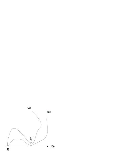
Figure 2: $P_{\textrm{left}}$ as $t\rightarrow\infty$

from which it can be seen that the limit $t\rightarrow\infty$ should have the exponent corresponding to a four-leg operator on the real axis, namely $\tilde{x}_{4}=h_{5}=24/\kappa-2$.

Recall from the argument below Eq. (13), that

$$P=\int_{c}^{t}{Q(t^{\prime})\textrm{d}t^{\prime}}\,,$$

with $Q(t)$ given in Eq. (14) and $c$ a constant, to be determined by the boundary conditions. In order to apply the boundary conditions at large $t$, the hypergeometric functions must be analytically continued for $|t|>1$, see for example $15.3.8$ in [18]. The expression for $P$ then takes the form

$$P(t) =A\int_{c}^{t}\Big{[}\frac{\Gamma(\frac{1}{2})\Gamma(\frac{1}{2}-\frac{8}{\kappa})}{\Gamma(1-\frac{4}{\kappa})\Gamma(-\frac{4}{\kappa})}\frac{1}{(1+u^{2})^{\frac{12}{\kappa}-\frac{1}{2}}}\,_{2}F_{1}(\frac{1}{2}+\frac{4}{\kappa},\frac{4}{\kappa}-\frac{1}{2};\frac{8}{\kappa}+\frac{1}{2};\frac{1}{1+u^{2}})$$

$$+\frac{\Gamma(\frac{1}{2})\Gamma(\frac{8}{\kappa}-\frac{1}{2})}{\Gamma(\frac{1}{2}+\frac{4}{\kappa})\Gamma(\frac{4}{\kappa}-\frac{1}{2})}\frac{1}{(1+u^{2})^{\frac{4}{\kappa}}}\,_{2}F_{1}(1-\frac{4}{\kappa},-\frac{4}{\kappa};-\frac{8}{\kappa}+\frac{3}{2};\frac{1}{1+u^{2}})$$

$$+B\frac{\Gamma(\frac{3}{2})\Gamma(\frac{1}{2}-\frac{8}{\kappa})}{\Gamma(\frac{3}{2}-\frac{4}{\kappa})\Gamma(\frac{1}{2}-\frac{4}{\kappa})}\frac{u}{(1+u^{2})^{\frac{12}{\kappa}}}\,_{2}F_{1}(1+\frac{4}{\kappa},\frac{4}{\kappa};\frac{1}{2}+\frac{8}{\kappa};\frac{1}{1+u^{2}})$$

$$+B\frac{\Gamma(\frac{3}{2})\Gamma(\frac{8}{\kappa}-\frac{1}{2})}{\Gamma(1+\frac{4}{\kappa})\Gamma(\frac{4}{\kappa})}\frac{u}{(1+u^{2})^{\frac{4}{\kappa}+\frac{1}{2}}}\,_{2}F_{1}(\frac{3}{2}-\frac{4}{\kappa},\frac{1}{2}-\frac{4}{\kappa};\frac{3}{2}-\frac{8}{\kappa};\frac{1}{1+u^{2}})\Big{]}\textrm{d}u\,.$$

The first and third terms in this large $t$ expansion approach zero as $t^{2-24/\kappa}$, while the second and fourth term approach zero as $t^{1-8/\kappa}$. For the range $0<\kappa<8$, which is the range of physical interest, the first and third terms fall off more quickly with increasing $t$. In order to satisfy the second boundary condition, the coefficients of the dominant second and fourth terms must ensure cancellation as $t\rightarrow\infty$. This uniquely determines the constant $B$ as

$$B=-2\frac{\Gamma(1+\frac{4}{\kappa})\Gamma(\frac{4}{\kappa})}{\Gamma(\frac{1}{2}+\frac{4}{\kappa})\Gamma(-\frac{1}{2}+\frac{4}{\kappa})}\,.$$

The solution follows immediately,

$$P_{\textrm{left}}(t)=\frac{\int_{t}^{\infty}{S(t^{\prime})\textrm{d}t^{\prime}}}{\int_{-\infty}^{\infty}{S(t^{\prime})\textrm{d}t^{\prime}}}\,,$$

where

$$S(t)=\frac{\,{}_{2}F_{1}(\frac{1}{2}+\frac{4}{\kappa},1-\frac{4}{\kappa};\frac{1}{2};-t^{2})-\frac{2\Gamma(1+\frac{4}{\kappa})\Gamma(\frac{4}{\kappa})}{\Gamma(\frac{1}{2}+\frac{4}{\kappa})\Gamma(-\frac{1}{2}+\frac{4}{\kappa})}\,t\,_{2}F_{1}(1+\frac{4}{\kappa},\frac{3}{2}-\frac{4}{\kappa};\frac{3}{2};-t^{2})}{(1+t^{2})^{\frac{8}{\kappa}-1}}\,.$$

It may be simplified using the identity

$$\int_{-\infty}^{\infty}{S(t^{\prime})\textrm{d}t^{\prime}}=\frac{2^{2-8/\kappa}\pi\Gamma(\frac{12}{\kappa}-1)}{\Gamma(\frac{4}{\kappa})\Gamma(\frac{8}{\kappa})}\,,$$

see for example Eq. ($7.512.10$) in [19]. The solution then takes the more elegant form

$$P_{\textrm{left}}(t)=\frac{\Gamma(\frac{4}{\kappa})\Gamma(\frac{8}{\kappa})}{2^{2-8/\kappa}\pi\Gamma(\frac{12}{\kappa}-1)}\int_{t}^{\infty}S(t^{\prime})\textrm{d}t^{\prime}\,.$$ (15)

It is a simple matter to derive $P_{\textrm{right}}$ since $P_{\textrm{right}}(t)=P_{\textrm{left}}(-t)$, thus

$$P_{\textrm{right}}(t)=\frac{\Gamma(\frac{4}{\kappa})\Gamma(\frac{8}{\kappa})}{2^{2-8/\kappa}\pi\Gamma(\frac{12}{\kappa}-1)}\int_{-t}^{\infty}S(t^{\prime})\textrm{d}t^{\prime}\,.$$ (16)

The remaining solution is $P_{\textrm{middle}}$. This can be derived in two ways. Firstly, for the total probability to be unity, $P_{\textrm{left}}+P_{\textrm{middle}}+P_{\textrm{right}}=1$. Subtracting the two previous solutions from one leads to

$$P_{\textrm{middle}}(t)=1-\frac{\Gamma(\frac{4}{\kappa})\Gamma(\frac{8}{\kappa})}{2^{2-8/\kappa}\pi\Gamma(\frac{12}{\kappa}-1)}\Big{[}\int_{t}^{\infty}S(t^{\prime})dt^{\prime}+\int_{-t}^{\infty}S(t^{\prime})dt^{\prime}\Big{]}\,.$$ (17)

Alternatively, the solution can be written as the integral of the odd term in $S(t)$ only, since we expect the solution to $P_{\textrm{middle}}$ to be an even function of $t$. Applying the boundary condition $P_{\textrm{middle}}(t\rightarrow\infty)=0$ determines $P_{\textrm{middle}}$ up to a multiplicative constant

$$P_{\textrm{middle}}(t)=D\Big{[}1-\frac{\int_{0}^{t}\frac{u}{(1+u^{2})^{\frac{8}{\kappa}-1}}\,_{2}F_{1}(1+\frac{4}{\kappa},\frac{3}{2}-\frac{4}{\kappa};\frac{3}{2};-u^{2})du}{\int_{0}^{\infty}\frac{u}{(1+u^{2})^{\frac{8}{\kappa}-1}}\,_{2}F_{1}(1+\frac{4}{\kappa},\frac{3}{2}-\frac{4}{\kappa};\frac{3}{2};-u^{2})du}\Big{]}\,.$$ (18)

The constant $D$ may be found by equating this expression with Equation (17) at $t=0$

$$D=1-\frac{\Gamma(\frac{4}{\kappa})\Gamma(\frac{8}{\kappa})}{2^{1-8/\kappa}\pi\Gamma(\frac{12}{\kappa}-1)}\int_{0}^{\infty}S(t^{\prime})dt^{\prime}\,.$$

Below, in Figure (3) are the results for $\kappa=8/3$, conjecturally corresponding to the scaling limit of two mutually avoiding self-avoiding walks starting near the origin, and $\kappa=6$, corresponding to the scaling limit of the percolation problem.

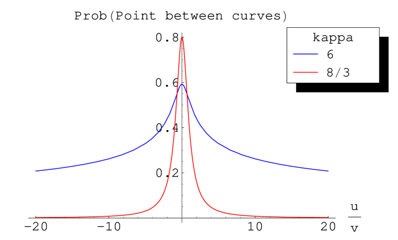
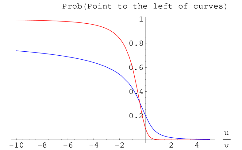
Figure 3: The self-avoiding walk ($\kappa=8/3$) and percolation ($\kappa=6$)

4 Special Cases

In the special cases $\kappa=0,2,8/3,4,8$, explicit solutions may be derived for $P_{\textrm{left}}$, $P_{\textrm{middle}}$ and $P_{\textrm{right}}$.

4.1 $\kappa=0$

With $\kappa=0$, the curves are deterministic straight lines. They start at the origin and proceed at an angle of $\pi/3$ radians from each other and from the real axis, as in Figure (4). Actually this is a rather singular limit of the equations, and the above result is more easily understood following the multiple SLE interpretation of Sec. 6.

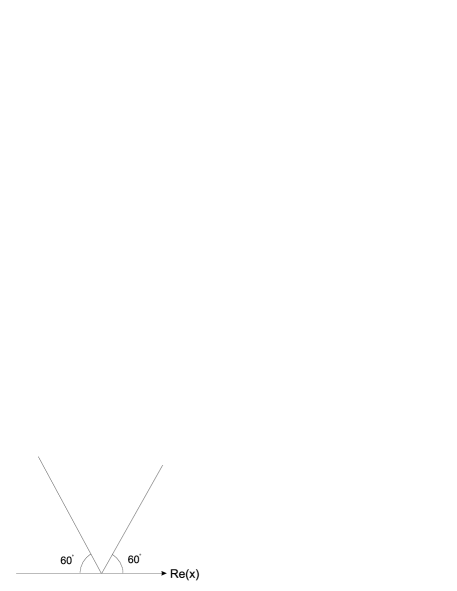
Figure 4: $\kappa=0$

4.2 $\kappa=2$

The solutions are written in terms of the function $S(t)$. In the case of $\kappa=2$, this takes the form

$$S(t) =\frac{1}{(1+t^{2})^{3}}\Big{[}\,_{2}F_{1}(\frac{5}{2},-1,\frac{1}{2},-t^{2})-\frac{32}{3\pi}t\,_{2}F_{1}(3,-\frac{1}{2},\frac{3}{2},-t^{2})\Big{]}$$

$$=\frac{1}{(1+t^{2})^{3}}\Big{[}1+5t^{2}-\frac{32t}{3\pi}\Big{(}\frac{t(13+15t^{2})+3(1+6t^{2}+5t^{4})\arctan(t)}{16(t+t^{3})}\Big{)}\Big{]}\,.$$

Inserting this expression into Eq. (15), (16) and (17) and performing the integrations, the following solutions are obtained

$$P_{\textrm{left}}(t) =\frac{1}{4}+\frac{1}{9\pi^{2}(1+t^{2})^{3}}\Big{[}(-16-9t^{2}+9t^{4})-9\pi(t^{3}+t^{5})$$

$$\quad+9(1+t^{2})\arctan(t)\Big{(}2t^{3}-\pi(1+t^{2})^{2}+(1+t^{2})^{2}\arctan(t)\Big{)}\Big{]}$$ (19)

$$P_{\textrm{right}}(t) =\frac{1}{4}+\frac{1}{9\pi^{2}(1+t^{2})^{3}}\Big{[}(-16-9t^{2}+9t^{4})+9\pi(t^{3}+t^{5})$$

$$\quad+9(1+t^{2})\arctan(t)\Big{(}2t^{3}+\pi(1+t^{2})^{2}+(1+t^{2})^{2}\arctan(t)\Big{)}\Big{]}$$ (20)

$$P_{\textrm{middle}}(t) =\frac{1}{2}-\frac{2}{9\pi^{2}(1+t^{2})^{3}}\Big{[}(-16-9t^{2}+9t^{4})$$

$$\quad+9(1+t^{2})\arctan(t)\Big{(}2t^{3}+(1+t^{2})^{2}\arctan(t)\Big{)}\Big{]}\,.$$ (21)

4.3 $\kappa=8/3$

Analytic solutions may be obtained for the special case of the scaling limit of two self-avoiding walks, conjectured to correspond to $\kappa=8/3$. In this case, the function $S(t)$ is given by

$$S(t) =\frac{1}{(1+t^{2})^{2}}\Big{[}\,_{2}F_{1}(2,-\frac{1}{2};\frac{1}{2};-t^{2})-\frac{3\pi t}{4}\Big{]}$$

$$=\frac{1}{(1+t^{2})^{2}}\Big{(}-\frac{1}{2(1+t^{2})}+\frac{3t}{2}\arctan(t)+\frac{3}{2}-\frac{3\pi t}{4}\Big{)}\,.$$

The solution for $P_{\textrm{left}}$ follows as

$$P_{\textrm{left}}(t) =\frac{\Gamma(\frac{4}{\kappa})\Gamma(\frac{8}{\kappa})}{2^{2-8/\kappa}\pi\Gamma(\frac{12}{\kappa}-1)}\int_{t}^{\infty}S(t^{\prime})\textrm{d}t^{\prime}$$

$$=\frac{16}{15\pi}\int_{t^{\prime}}^{\infty}{\frac{1}{(1+t^{\prime 2})^{2}}\Big{(}-\frac{1}{2(1+t^{\prime 2})}+\frac{3t^{\prime}}{2}\arctan(t^{\prime})+\frac{3}{2}-\frac{3\pi t^{\prime}}{4}\Big{)}\textrm{d}t^{\prime}}$$

$$=\frac{16}{15\pi}\Big{[}\frac{t^{\prime}(13+15t^{\prime 2})+3(1+6t^{\prime 2}+5t^{\prime 4})\arctan(t^{\prime})}{16(1+t^{\prime 2})^{2}}+\frac{3\pi}{8}\frac{1}{1+t^{\prime 2}}\Big{]}^{\infty}_{t}$$

$$=\frac{1}{2}-\frac{16}{15\pi}\frac{t(13+15t^{2})+3(1+6t^{2}+5t^{4})\arctan(t)}{16(1+t^{2})^{2}}-\frac{2}{5}\frac{1}{1+t^{2}}\,.$$

This may be simplified to

$$P_{\textrm{left}}(t)=\frac{-2t(13+15t^{2})+3\pi(1+6t^{2}+5t^{4})-6(1+6t^{2}+5t^{4})\arctan(t)}{30\pi(1+t^{2})^{2}}\,.$$ (22)

The other solutions are

$$P_{\textrm{right}}(t)=\frac{2t(13+15t^{2})+3\pi(1+6t^{2}+5t^{4})+6(1+6t^{2}+5t^{4})\arctan(t)}{30\pi(1+t^{2})^{2}}$$ (23)

$$P_{\textrm{middle}}(t)=\frac{4}{5(1+t^{2})}\,.$$ (24)

4.4 $\kappa=4$

With $\kappa=4$, $S(t)$ takes the form

$$S(t)=\frac{1}{1+t^{2}}\Big{[}\,_{2}F_{1}(\frac{3}{2},0,\frac{1}{2},-t^{2})+Bt\,_{2}F_{1}(2,\frac{1}{2},\frac{3}{2},-t^{2})\Big{]}\,,$$

where $B=-4/\pi$. Substituting for the hypergeometric functions in terms of elementary functions leads to

$$S(t)=\frac{1}{1+t^{2}}\Big{[}1-\frac{2t}{\pi}\Big{(}\frac{1}{1+t^{2}}+\frac{\arctan(t)}{t}\Big{)}\Big{]}\,.$$

Inserting this form into the expression for $P_{\textrm{left}}$

$$P_{\textrm{left}}(t)=\frac{1}{4}-\frac{1}{\pi^{2}(1+t^{2})}-\frac{\arctan(t)}{\pi}+\frac{\arctan^{2}(t)}{\pi^{2}}\,.$$ (25)

The other solutions are

$$P_{\textrm{right}}(t) =\frac{1}{4}-\frac{1}{\pi^{2}(1+t^{2})}+\frac{\arctan(t)}{\pi}+\frac{\arctan^{2}(t)}{\pi^{2}}$$ (26)

$$P_{\textrm{middle}}(t) =\frac{1}{2}+\frac{2}{\pi^{2}(1+t^{2})}-\frac{2\arctan^{2}(t)}{\pi^{2}}\,.$$ (27)

In terms of the angle $\phi$ from the imaginary axis to the point $\xi$, which is to say $\phi=\arctan(u/v)=\arctan(t)$,

$$P_{\textrm{left}}(\phi) =\frac{1}{4}-\frac{\textrm{cos}^{2}(\phi)}{\pi^{2}}-\frac{\phi}{\pi}+\frac{\phi^{2}}{\pi^{2}}$$

$$P_{\textrm{right}}(\phi) =\frac{1}{4}-\frac{\textrm{cos}^{2}(\phi)}{\pi^{2}}+\frac{\phi}{\pi}+\frac{\phi^{2}}{\pi^{2}}$$

$$P_{\textrm{middle}}(\phi) =\frac{1}{2}+\frac{2\cos^{2}(\phi)}{\pi^{2}}-\frac{2\phi^{2}}{\pi^{2}}\,.$$

4.5 $\kappa=8$

The case $\kappa=8$ is subtle and requires careful treatment. For the single curve, taking the limit as $\kappa\to 8-$ at fixed $t$ yields an expression which fails to satisfy the boundary conditions [9]. Instead, the probability of any point not on the real axis being to one side of the curve is everywhere equal to a half. This however makes physical sense since for $\kappa=8$ the curve is space-filling.

For the case of two curves there is a similar boundary condition violating solution which is obtained by continuing the general solution for finite $t$ to $\kappa=8$. There is a second solution, however, which follows from solving the differential equations at $\kappa=8$ and which does satisfy the boundary conditions.

First, consider the general solution in the limit $\kappa\rightarrow 8$. Using the usual definition

$$S(t)=\frac{\,{}_{2}F_{1}(\frac{1}{2}+\frac{4}{\kappa},1-\frac{4}{\kappa};\frac{1}{2};-t^{2})-\frac{2\Gamma(1+\frac{4}{\kappa})\Gamma(\frac{4}{\kappa})}{\Gamma(\frac{1}{2}+\frac{4}{\kappa})\Gamma(-\frac{1}{2}+\frac{4}{\kappa})}\,t\,_{2}F_{1}(1+\frac{4}{\kappa},\frac{3}{2}-\frac{4}{\kappa};\frac{3}{2};-t^{2})}{(1+t^{2})^{\frac{8}{\kappa}-1}}\,,$$

the solution is

$$P_{\textrm{left}}(t) =\frac{\int_{t}^{\infty}{S(t^{\prime})\textrm{d}t^{\prime}}}{\int_{-\infty}^{\infty}{S(t^{\prime})\textrm{d}t^{\prime}}}$$

$$=\frac{\Gamma(\frac{4}{\kappa})\Gamma(\frac{8}{\kappa})}{2^{2-8/\kappa}\pi\Gamma(\frac{12}{\kappa}-1)}\int_{t}^{\infty}S(t^{\prime})\textrm{d}t^{\prime}\,.$$

In anticipation of taking the limit $\kappa\rightarrow 8$, define $\kappa=8-\epsilon$ and assume that $\epsilon$ is small. Rewriting the above expressions in terms of $\epsilon$:

$$S(t)=\frac{\,{}_{2}F_{1}(1+\frac{\epsilon}{16},\frac{1}{2}-\frac{\epsilon}{16};\frac{1}{2};-t^{2})-\frac{2\Gamma(\frac{3}{2}+\frac{\epsilon}{16})\Gamma(\frac{1}{2}+\frac{\epsilon}{16})}{\Gamma(1+\frac{\epsilon}{16})\Gamma(\frac{\epsilon}{16})}\,t\,_{2}F_{1}(\frac{3}{2}+\frac{\epsilon}{16},1-\frac{\epsilon}{16};\frac{3}{2};-t^{2})}{(1+t^{2})^{\frac{\epsilon}{8}}}$$

$$P_{\textrm{left}}(t)=\frac{\Gamma(\frac{1}{2}+\frac{\epsilon}{16})\Gamma(1+\frac{\epsilon}{8})}{2^{1-\frac{\epsilon}{8}}\pi\Gamma(\frac{1}{2}+\frac{3\epsilon}{16})}\int_{t}^{\infty}S(t^{\prime})\textrm{d}t^{\prime}\,.$$

The two hypergeometric functions in $S(t)$ can be analytically continued for $t>0$

$$S(t)=\frac{\sqrt{\pi}\Gamma(-\frac{1}{2}-\frac{\epsilon}{8})}{\Gamma(\frac{1}{2}-\frac{\epsilon}{16})\Gamma(-\frac{1}{2}-\frac{\epsilon}{16})}\frac{1}{(1+t^{\prime 2})^{1+\frac{3\epsilon}{16}}}\,_{2}F_{1}(1+\frac{\epsilon}{16},\frac{\epsilon}{16};\frac{3}{2}+\frac{\epsilon}{8};\frac{1}{1+t^{\prime 2}})$$

$$+\frac{\sqrt{\pi}\Gamma(\frac{1}{2}+\frac{\epsilon}{8})}{\Gamma(1+\frac{\epsilon}{16})\Gamma(\frac{\epsilon}{16})}\frac{1}{(1+t^{\prime 2})^{\frac{1}{2}+\frac{\epsilon}{16}}}\,_{2}F_{1}(\frac{1}{2}-\frac{\epsilon}{16},-\frac{1}{2}-\frac{\epsilon}{16};\frac{1}{2}-\frac{\epsilon}{8};\frac{1}{1+t^{\prime 2}})$$

$$-\sqrt{\pi}\frac{\Gamma(\frac{3}{2}+\frac{\epsilon}{16})\Gamma(\frac{1}{2}+\frac{\epsilon}{16})\Gamma(-\frac{1}{2}-\frac{\epsilon}{8})}{\Gamma(1+\frac{\epsilon}{16})\Gamma(\frac{\epsilon}{16})\Gamma(1-\frac{\epsilon}{16})\Gamma(-\frac{\epsilon}{16})}\frac{t^{\prime}\,_{2}F_{1}(\frac{3}{2}+\frac{\epsilon}{16},\frac{1}{2}+\frac{\epsilon}{16};\frac{3}{2}+\frac{\epsilon}{8};\frac{1}{1+t^{\prime 2}})}{(1+t^{\prime 2})^{\frac{3}{2}+\frac{3\epsilon}{16}}}$$

$$-\sqrt{\pi}\frac{\Gamma(\frac{1}{2}+\frac{\epsilon}{8})}{\Gamma(1+\frac{\epsilon}{16})\Gamma(\frac{\epsilon}{16})}\frac{t^{\prime}\,_{2}F_{1}(1-\frac{\epsilon}{16},-\frac{\epsilon}{16};\frac{1}{2}-\frac{\epsilon}{8};\frac{1}{1+t^{\prime 2}})}{(1+t^{\prime 2})^{1+\frac{\epsilon}{16}}}\,.$$

Each of these four terms are to be integrated from $t^{\prime}=t$ to $\infty$. This can be done by expanding the hypergeometric functions and integrating term by term. Consider the integral of the first function in $S(t)$ for $t>0$

$$\frac{\sqrt{\pi}\Gamma(-\frac{1}{2}-\frac{\epsilon}{8})}{\Gamma(\frac{1}{2}-\frac{\epsilon}{16})\Gamma(-\frac{1}{2}-\frac{\epsilon}{16})}\int_{t}^{\infty}{\frac{1}{(1+t^{\prime 2})^{1+\frac{3\epsilon}{16}}}\,_{2}F_{1}(1+\frac{\epsilon}{16},\frac{\epsilon}{16};\frac{3}{2}+\frac{\epsilon}{8};\frac{1}{1+t^{\prime 2}})}\textrm{d}t^{\prime}$$

$$=\frac{\sqrt{\pi}\Gamma(-\frac{1}{2}-\frac{\epsilon}{8})}{\Gamma(\frac{1}{2}-\frac{\epsilon}{16})\Gamma(-\frac{1}{2}-\frac{\epsilon}{16})}\int_{t}^{\infty}{\frac{1}{(1+t^{\prime 2})^{1+\frac{3\epsilon}{16}}}\Big{[}1+\frac{(1+\frac{\epsilon}{16})(\frac{\epsilon}{16})}{(\frac{3}{2}+\frac{\epsilon}{8})1!}\frac{1}{1+t^{2}}+\ldots\Big{]}}\textrm{d}t^{\prime}$$

$$=\frac{\sqrt{\pi}\Gamma(-\frac{1}{2}-\frac{\epsilon}{8})}{\Gamma(\frac{1}{2}-\frac{\epsilon}{16})\Gamma(-\frac{1}{2}-\frac{\epsilon}{16})}\int_{t}^{\infty}{\frac{1}{(1+t^{\prime 2})^{1+\frac{3\epsilon}{16}}}\textrm{d}t^{\prime}}+\epsilon f(\epsilon,t)$$

$$=-t\,_{2}F_{1}(\frac{1}{2},1+\frac{3\epsilon}{16};\frac{3}{2};-t^{2})+\frac{\sqrt{\pi}\Gamma(\frac{1}{2}+\frac{3\epsilon}{16})}{2\Gamma(1+\frac{3\epsilon}{16})}+\epsilon f(t,\epsilon)\,,$$

where $f(\epsilon,t)$ is a convergent function of its arguments for all $t$ in the limit $\epsilon\rightarrow 0$.

After integration, the third term gives $\epsilon^{2}g(\epsilon,t)$, where $g(\epsilon,t)$ is also a convergent function of its arguments for all $t$ in the limit $\epsilon\rightarrow 0$.

The integral of the second and fourth terms should be considered together. They contribute

$$\frac{\sqrt{\pi}\Gamma(\frac{1}{2}+\frac{\epsilon}{8})}{\Gamma(1+\frac{\epsilon}{16})\Gamma(\frac{\epsilon}{16})}\int_{t}^{\infty}{\Big{[}\frac{1}{(1+t^{\prime 2})^{\frac{1}{2}+\frac{\epsilon}{16}}}-\frac{t^{\prime}}{(1+t^{\prime 2})^{1+\frac{\epsilon}{16}}}\Big{]}\textrm{d}t^{\prime}}+\epsilon h(\epsilon,t)\,,$$

where $h(\epsilon,t)$ is a convergent function for all $t$ in the limit $\epsilon\rightarrow 0$. The integral of $S(t)$ is therefore

$$\int_{t}^{\infty}{S(t^{\prime})\textrm{d}t^{\prime}}=-t\,_{2}F_{1}(\frac{1}{2},1+\frac{3\epsilon}{16};\frac{3}{2};-t^{2})+\frac{\sqrt{\pi}\Gamma(\frac{1}{2}+\frac{3\epsilon}{16})}{2\Gamma(1+\frac{3\epsilon}{16})}+\epsilon f(t,\epsilon)+\epsilon^{2}g(t,\epsilon)$$

$$\qquad\qquad+\frac{\sqrt{\pi}\Gamma(\frac{1}{2}+\frac{\epsilon}{8})}{\Gamma(1+\frac{\epsilon}{16})\Gamma(\frac{\epsilon}{16})}\int_{t}^{\infty}{\Big{[}\frac{1}{(1+t^{\prime 2})^{\frac{1}{2}+\frac{\epsilon}{16}}}-\frac{t^{\prime}}{(1+t^{\prime 2})^{1+\frac{\epsilon}{16}}}\Big{]}\textrm{d}t^{\prime}}+\epsilon h(\epsilon,t)\,.$$

Taking the limit $\epsilon\rightarrow 0$, the first two terms become

$$-\arctan(t)+\frac{\pi}{2}$$

and the terms involving $f(\epsilon,t),g(\epsilon,t),h(\epsilon,t)$ have coefficients which tend to the zero. The remaining term is

$$\lim_{\epsilon\rightarrow 0}{\frac{\sqrt{\pi}\Gamma(\frac{1}{2}+\frac{\epsilon}{8})}{\Gamma(1+\frac{\epsilon}{16})\Gamma(\frac{\epsilon}{16})}\int_{t}^{\infty}{\Big{[}\frac{1}{(1+t^{\prime 2})^{\frac{1}{2}+\frac{\epsilon}{16}}}-\frac{t^{\prime}}{(1+t^{\prime 2})^{1+\frac{\epsilon}{16}}}\Big{]}\textrm{d}t^{\prime}}}\,,$$

where $j(\epsilon,t)$ is a convergent function of its arguments for all $t$ in the limit $\epsilon\rightarrow 0$. The integral is finite, so the expression goes to zero as $\epsilon\rightarrow 0$.

Using

$$\lim_{\epsilon\rightarrow 0}{\frac{\Gamma(\frac{1}{2}+\frac{\epsilon}{16})\Gamma(1+\frac{\epsilon}{8})}{2^{1-\frac{\epsilon}{8}}\pi\Gamma(\frac{1}{2}+\frac{3\epsilon}{16})}=\frac{1}{2\pi}}\,,$$

allows the solution for $P_{\textrm{left}}(t)$ and related expressions to be deduced in terms of the angle $\phi$ defined in the previous subsection,

$$P_{\textrm{left}}(\phi) =\frac{1}{4}-\frac{\phi}{2\pi}\,,$$ (28)

$$P_{\textrm{right}}(\phi) =\frac{1}{4}+\frac{\phi}{2\pi}\,,$$ (29)

$$P_{\textrm{middle}}(\phi) =\frac{1}{2}\,.$$ (30)

Note that these are valid only for $\phi\not=\pm\pi/2$. The limits $\kappa\to 8$ and $|t|\to\infty$ do not commute.

Now take $\kappa=8$ from the beginning. The differential equation has solutions of the form

$$P_{\textrm{left}}(t)=A\arctan(t)+B\,.$$

If $A$ and $B$ are chosen to be $-1/\pi$ and $1/2$ respectively, this satisfies the boundary conditions. Then in terms of the angle $\phi$,

$$P_{\textrm{left}}(\phi) =\frac{1}{2}-\frac{\phi}{\pi}\,,$$ (31)

$$P_{\textrm{right}}(\phi) =\frac{1}{2}+\frac{\phi}{\pi}\,,$$ (32)

$$P_{\textrm{middle}}(\phi) =0\,.$$ (33)

This is not the analytic continuation of the first solution to $\kappa=8$. Mathematically, this may be traced to the fact that the limits $\kappa\to 8-$ and $t\to+\infty$ do not commute, yet we have to impose the boundary condition on $P_{\textrm{left}}$ at $t=+\infty$.

Physically, these two solutions appear to lead to different pictures. In the first case, the probability that a given point lies between the two curves is exactly $\frac{1}{2}$. This may be understood in terms of the physical picture of the curves being the boundaries of two disjoint uniform spanning clusters which are separated by some random simple curve $\gamma_{\rm sep}$. Each curve fills the entire region to the left(right) of $\gamma_{\rm sep}$. Within each region, the probability that a given point lies to the left(right) of the curve is $\frac{1}{2}$ as before, but the probability that it lies in this region, to the left(right) of the separatrix is $\frac{1}{2}(1\mp 2\phi/\pi)$. Thus the probability that a point lies to the left of both curves is $\frac{1}{2}\cdot\frac{1}{2}(1-2\phi/\pi)$, while the probability this it lies between them is

$$\frac{1}{2}\cdot\frac{1}{2}(1-2\phi/\pi)+\frac{1}{2}\cdot\frac{1}{2}(1+2\phi/\pi)=\frac{1}{2}\,.$$ (34)

In the second solution, the probability that a point is between the curves is zero, hence the area between them vanishes. Physically, this could correspond to two mutually avoiding dense polymers, which also correspond to $\kappa=8$. In this case, however, they find it entropically favourable closely to follow each other. The probability that a point lies to one side of this composite curve is the same as for a single curve with $\kappa=4$, see [9]. This may be understood in terms of the stochastic interpretation of Sec. 6. For $\kappa=8$ the points $x_{1}$ and $x_{2}$ almost certainly collide in finite time, after which it is necessary to prescribe how to continue the solution. One possibility is that the two points coalesce, in which case their centre of mass describes a Brownian motion with $\kappa^{\prime}=\frac{1}{2}\kappa=4$, as in the second solution. Another possibility is that they are conditioned never to collide, which then presumably corresponds to the first case.

5 Application to the quantum Hall transition

The Quantum Hall effect is observed in two dimensional electron gases in semiconductors with magnetic fields applied normal to the plane. Donor ions are spatially separated from the electron gas in order to increase the mobility of the electrons in the sample. The ions are positively charged and the resulting Coulomb potential in the electron gas can be modelled as a random potential, $V$. A semi-classical approximation may be used in the limits of slowly varying potential on the scale of the magnetic length $l=\sqrt{\hbar c/eB}$ and strong magnetic field, defined as

$$\hbar\omega_{c}\equiv\frac{\hbar eB}{mc}\ll\epsilon_{F}\,,$$

where $\epsilon_{F}$ is the Fermi energy of the system. In this limit, the eigenfunctions of electrons are large only around constant energy surfaces of the potential, $V$, see [21]. The eigenfunctions can be approximated by

$$\psi(u,v)=C(u)\chi_{n}(v)e^{i\phi(u,v)}\,,$$

where $u$ is the length along the constant energy surface and $v$ is the distance normal to it. $C$ is a normalisation factor and $\chi_{n}$ is the $n$th harmonic oscillator function

$$\chi_{n}=H_{n}(\frac{v}{l})e^{-\frac{v^{2}}{2l^{2}}}\,.$$

Choose the zero of the random potential to be the spatial average of the potential and assume that $\langle V(r)V(r+\delta r)\rangle$ goes to zero for $\delta r\gg b$. The requirement that the potential varies slowly compared to the magnetic length is equivalent to $b>>l$. If all points where the potential is greater than a value $E$ are coloured white and points where $V\leq E$ are coloured black, the lines of constant potential will be given by the boundary between the two coloured regions. This model is believed to be in the same universality class as lattice percolation. Thus, electrons will move along the boundaries of percolation clusters. In general, the boundaries will form closed loops, but for the critical value $E=0$, their mean size diverges and they will be locally described by SLE with $\kappa=6$. The appropriate boundary conditions for the percolation picture are that the top and bottom edges should be coloured white since the potential is effectively infinite there.

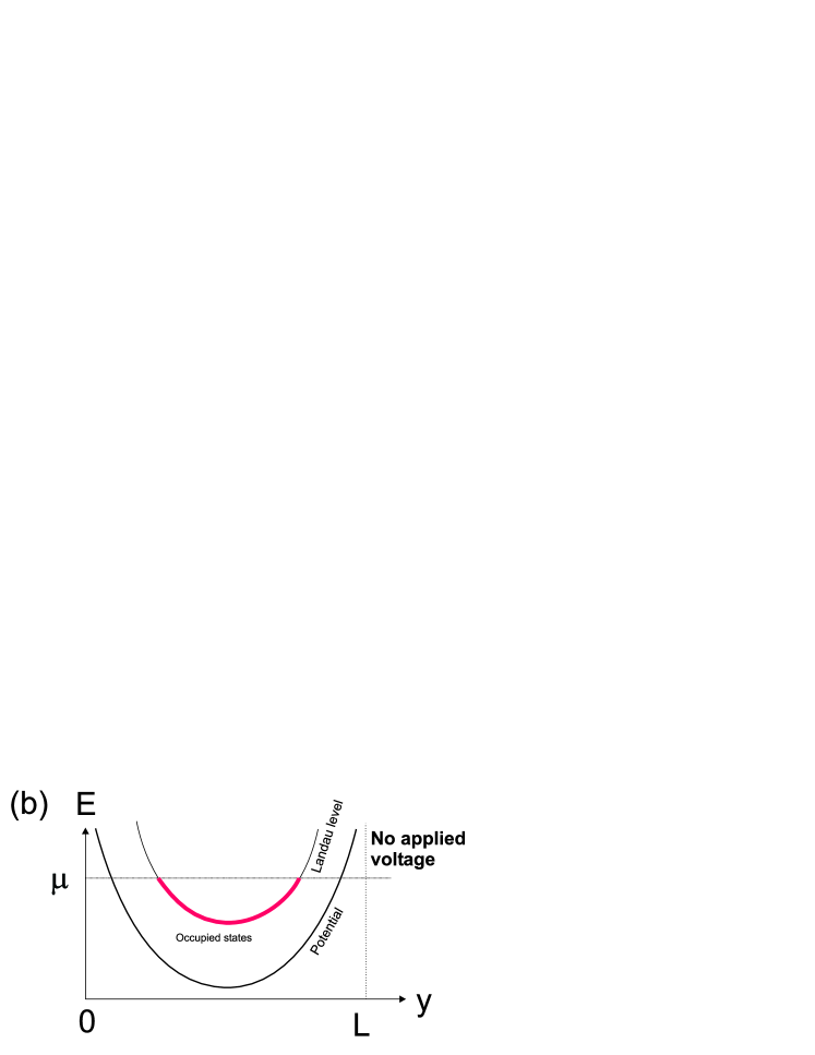
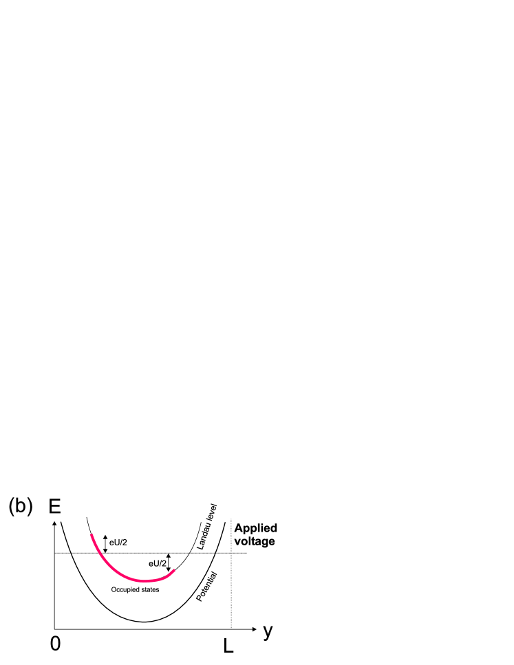
Figure 5: The spatial distribution of eigenstates, showing occupation before and after a potential difference is applied between the ends of the sample.

As a function of $y$, the distance across the sample, the energy of the Landau levels follow the form of the potential and those states with $E\leq\mu$, the chemical potential, are occupied, as shown in Figure (5a). Diamagnetic currents flow, both around the closed loops and along the extended cluster boundaries with $E=0$, as shown in Figure (6a). On connection of the leads to the ends and the application of a potential difference, the current distribution will change from that of the equilibrium case.

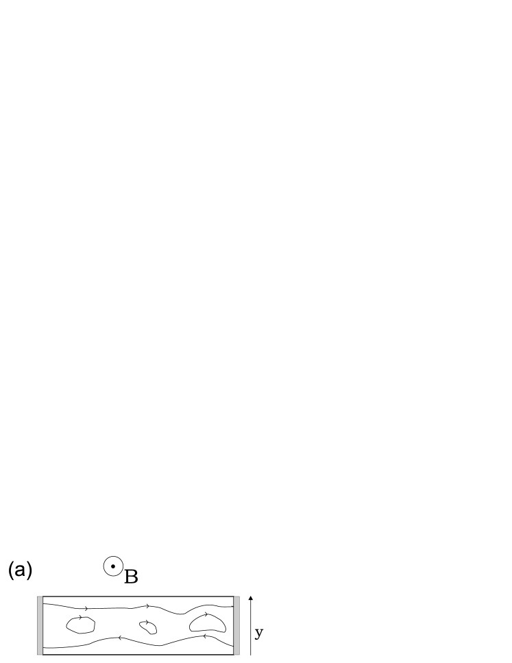
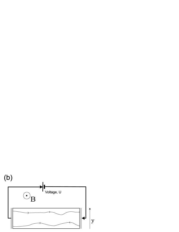
Figure 6: The top diagram depicts the diamagnetic currents. The figure below shows the Hall bar with leads attached and a voltage applied. The arrows in both diagrams represent the direction of electron flow.

The currents flowing along the extended cluster boundaries will be affected the most, since these are the only paths which can carry a net current along the length of the sample without potential tunnelling. The Fermi energy of electrons moving along the bottom cluster will be the equilibrium level plus $eU/2$, since these electrons flow from the electron reservoir at the negative battery contact. The Fermi energy of the electrons in the upper cluster boundary will be that of the equilibrium case minus $eU/2$, since these electrons flow from the electron reservoir at the positive battery contact. Relative to the equilibrium case, therefore, an extra current, $\delta I$ flows along the lower cluster boundary and, to a first approximation, $\delta I$ less current flows along the upper cluster boundary. The averaged change in the current distribution, compared to the equilibrium case, will be given by the spatial average of the extended cluster boundaries in the percolation picture ($\kappa=6$). We may relate the strip geometry of the Hall bar experiment to the half-plane discussed in this paper by the conformal mapping $z\rightarrow z^{\prime}=w(z)$ with

$$w(z)=\frac{L}{\pi}\ln(z)\,,$$

which maps the upper half plane to an infinite strip of width $L$. Lines with constant angle, parametrised by their value of $t=u/v$, are mapped to lines of constant distance, $y$, from the bottom of the infinite strip, given by

$$y=\frac{L}{\pi}\arctan(\frac{1}{t})\,.$$

A little thought then shows that the mean extra current density flowing along the upper boundary curve at height $y$ in the sample is proportional to the derivative with respect to $y$ of the probability that $y$ is above both curves. Similarly, the extra current density flowing along the lower curve is $-\textrm{d}P_{\textrm{below}}/\textrm{d}y$. Thus,

$$I \propto\frac{\textrm{d}P_{\textrm{left}}}{\textrm{d}y}-\frac{\textrm{d}P_{\textrm{right}}}{\textrm{d}y}$$

$$\propto-\frac{\Gamma(\frac{4}{\kappa})\Gamma(\frac{8}{\kappa})}{2^{2-8/\kappa}\pi\Gamma(\frac{12}{\kappa}-1)}\frac{\pi}{L}(1+\frac{1}{\tan(\frac{\pi y}{L})^{2}})\Big{[}S(\frac{1}{\tan(\frac{\pi y}{L})})+S(\frac{1}{\tan(\pi-\frac{\pi y}{L})})\Big{]}\,,$$

where, as previously,

$$S(t)=\frac{\,{}_{2}F_{1}(\frac{1}{2}+\frac{4}{\kappa},1-\frac{4}{\kappa};\frac{1}{2};-t^{2})-\frac{2\Gamma(1+\frac{4}{\kappa})\Gamma(\frac{4}{\kappa})}{\Gamma(\frac{1}{2}+\frac{4}{\kappa})\Gamma(-\frac{1}{2}+\frac{4}{\kappa})}\,t\,_{2}F_{1}(1+\frac{4}{\kappa},\frac{3}{2}-\frac{4}{\kappa};\frac{3}{2};-t^{2})}{(1+t^{2})^{\frac{8}{\kappa}-1}}\,.$$

For $\kappa=6$ this becomes

$$I\propto\frac{\Gamma(\frac{2}{3})\Gamma(\frac{4}{3})}{2^{2/3}L}(1+\frac{1}{\tan(\frac{\pi y}{L})^{2}})\Big{[}S(\frac{1}{\tan(\frac{\pi y}{L})})+S(\frac{1}{\tan(\pi-\frac{\pi y}{L})})\Big{]}\,,$$

with

$$S(t)=\frac{\,{}_{2}F_{1}(\frac{5}{6},\frac{2}{3};\frac{1}{2};-t^{2})-\frac{2\Gamma(\frac{5}{3})\Gamma(\frac{2}{3})}{\Gamma(\frac{7}{6})\Gamma(\frac{1}{6})}\,t\,_{2}F_{1}(\frac{5}{3},\frac{5}{6};\frac{3}{2};-t^{2})}{(1+t^{2})^{\frac{1}{3}}}\,.$$

A plot of the mean current distribution is presented in Figure (7).

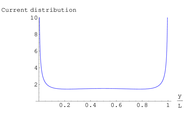
Figure 7: Average current distribution for the continuum percolation model

There are two important potential limitations on the applicability of this result: (i) we have ignored Coulomb interactions between electrons, which, although they are often assumed not to change the single-electron picture of the plateaux transition, may well affect the current distribution; (ii) we have neglected quantum tunnelling between neighbouring regions of zero potential, which are believed to be relevant and to change the universality class away from classical percolation. However, for the spin quantum Hall transition[23, 24] this is not the case.

6 Reverse Engineering SLE$(\kappa,2)$

Now let us consider the more general case of two curves starting at the points $x_{1}\neq x_{2}$. $P_{\textrm{left}}$, $P_{\textrm{middle}}$ and $P_{\textrm{right}}$ are given by the ratio of correlation functions

$$P(x_{1},x_{2},\xi) =\frac{\langle\Phi(\xi)\phi_{2}(x_{1})\phi_{2}(x_{2})\phi_{2}(\infty)\phi_{2}(\infty)\rangle}{\langle\phi_{2}(x_{1})\phi_{2}(x_{2})\phi_{2}(\infty)\phi_{2}(\infty)\rangle}\equiv\frac{F_{\Phi}(x_{1},x_{2},\xi)}{F_{\textbf{1}}(x_{1},x_{2})}\,,$$

Using the following definition of the differential operator $D_{1}$:

$$D_{1}\equiv\Big{[}\frac{\kappa}{4}\frac{\partial^{2}}{\partial x_{1}^{2}}-\frac{h_{2,1}}{(x_{2}-x_{1})^{2}}+\frac{1}{x_{2}-x_{1}}\frac{\partial}{\partial x_{2}}\Big{]}\,,$$

$F_{\Phi}$ satisfies the BPZ differential equation

$$D_{1}F_{\Phi}(x_{1},x_{2},\Phi) =<\langle\delta_{x_{1}}\Phi(\xi)\phi_{2}(x_{1})\phi_{2}(x_{2})\phi_{2}^{2}(\infty)\rangle\,,$$

$$\textrm{with}\quad\delta_{x_{1}}=\frac{1}{\xi-x_{1}}\,.$$

Writing $F_{\Phi}=P(x_{1},x_{2},\Phi)F_{\textbf{1}}(x_{1},x_{2})$ and using $D_{1}F_{\textbf{1}}(x_{1},x_{2})=0$ ,

$$D_{1}P(x_{1},x_{2},\Phi)+\frac{\kappa}{2F_{\textbf{1}}(x_{1},x_{2})}\frac{\partial F_{\textbf{1}}(x_{1},x_{2})}{\partial x_{1}}\frac{\partial P(x_{1},x_{2},\Phi)}{\partial x_{1}}=\delta_{x_{1}}P(x_{1},x_{2},\Phi)\,.$$ (35)

$F_{\textbf{1}}(x_{1},x_{2})$ is a three point function. This can be seen by taking the fusion of the operators at infinity, ie $\phi_{2}^{2}(\infty)=\phi_{3}(\infty)$. Conformal field theory may be employed to fix the form of the three point function up to a constant

$$F_{\textbf{1}}(x_{1},x_{2})=\frac{c}{|x_{1}-x_{2}|^{2h_{2,1}-h_{3,1}}}=\frac{c}{|x_{1}-x_{2}|^{-2/\kappa}}\,.$$

From this expression for $F_{\textbf{1}}(x_{1},x_{2})$, it can be seen that

$$\frac{\partial F_{\textbf{1}}(x_{1},x_{2})}{\partial x_{1}}=\frac{2}{\kappa}\frac{F_{\textbf{1}}(x_{1},x_{2})}{|x_{1}-x_{2}|}\,.$$

Substituting this into Eq. (35), we obtain

$$\Big{[}\frac{\kappa}{2}\frac{\partial}{\partial x_{1}^{2}}+\frac{2}{x_{1}-x_{2}}(\frac{\partial}{\partial x_{2}}-\frac{\partial}{\partial x_{1}})\Big{]}G(x_{1},x_{2},\Phi)=\delta_{x_{1}}G(x_{1},x_{2},\Phi)\,.$$ (36)

This has the form of the adjoint Fokker-Planck equation corresponding to the stochastic process

$$dx_{1} =\sqrt{\kappa}dB_{t}+\frac{2}{x_{1}-x_{2}}dt$$

$$dx_{2} =\frac{2}{x_{2}-x_{1}}dt\,.$$ (37)

This is called SLE$(\kappa,2)$ [25]. Since the differential equation resulting from this choice of stochastic variables is the same as the CFT solution to the 2 curve problem, we conjecture that this stochastic process gives the driving term in the Loewner equation for one curve, given the existence of the other. Recently Dubédat[26] has argued that such a description follows from the requirement that the generators of the Loewner processes for the two curves should commute.

It is interesting to take $\kappa=0$, which results in a deterministic Loewner equation with analytic solution. Solving Eq. (37) yields the following forcing function

$$x_{1}=\sqrt{2t+\frac{\delta^{2}}{4}}\,,$$ (38)

where $t$ parametrises distance along the curve and $\delta$ is the distance between the starting points of the curves on the real axis. Kadanoff et al. derived solutions to the Loewner equation for various driving terms [27], including $x_{1}\propto\sqrt{t}$. The solution below is similar to the case of a square root forcing term. The mapping from the upper half plane with boundary curves grown up to time $t$ back to the upper half plane $g_{t}$ is the solution to the Loewner equation

$$\frac{\textrm{d}g_{t}(z)}{\textrm{d}t}=\frac{2}{g_{t}(z)-\sqrt{2t+\frac{\delta^{2}}{4}}}$$ (39)

subject to the boundary condition $g_{t=0}(z)=z$. A change of variables to

$$G_{t}=\frac{g_{t}}{\sqrt{\frac{\delta^{2}}{8}+t}}\,,\quad\tau=\ln(\frac{\delta^{2}}{8}+t)\,,$$

leads to the equation

$$\frac{\textrm{d}G}{\textrm{d}\tau}=\frac{(G-y_{+})(G-y_{-})}{2(\sqrt{2}-G)}\,,$$ (40)

with $y_{+}=2\sqrt{2}$ and $y_{-}=-\sqrt{2}$. In terms of

$$H(G)=\frac{4\sqrt{2}\ln(G+\sqrt{2})+2\sqrt{2}\ln(G-2\sqrt{2})}{3\sqrt{2}}\,,$$ (41)

the equation may be written

$$\frac{\textrm{d}H}{\textrm{d}\tau}=-1\,,$$

with solution

$$-H(\frac{g_{t}}{\sqrt{t+\frac{\delta^{2}}{8}}})=\ln(\frac{\delta^{2}}{8}+t)+\textrm{const}\,.$$

The constant may be set by the requirement that $g_{t=0}(z)=z$, then

$$-H(\frac{g_{t}}{\sqrt{t+\frac{\delta^{2}}{8}}})=\ln(1+\frac{8t}{\delta^{2}})-H(\frac{2\sqrt{2}z}{\delta})\,.$$ (42)

The boundary curves $z_{c}(t)$ are the line of singularities which are found by setting $g_{t}(z)=\sqrt{2}\sqrt{t+\delta^{2}/8}$, namely

$$-H(\sqrt{2})=\ln(1+\frac{8t}{\delta^{2}})-H(\frac{2\sqrt{2}z_{c}(t)}{\delta})\,.$$ (43)

After substitution for $H(G)$ this may be simplified to

$$4(\frac{z_{c}(t)}{\delta})^{3}-3\frac{z_{c}(t)}{\delta}+f(t)=0\,,$$

with $f(t)=2(1+8t/\delta)^{3/2}-1$. The solutions are hyperbole of the form

$$4a^{2}-\frac{4}{3}b^{2}=\delta^{2}\,,$$ (44)

where the location of the tip is given by $z_{c}=a+ib$. The limit $\delta\rightarrow 0$ is the case which we have quoted in Sec. 4.1. In this limit, the curve is a straight line, proceeding at an angle of $\pi/3$ from the positive real axis. By symmetry, the other curve is also a straight line, making an angle of $\pi/3$ from the negative real axis. Figure (4) displays the solution.

7 Summary

This paper has described how the conformal field theoretic treatment of SLE may be generalised to two curves. In the limit that both curves originate from the same point, the equations for the probability that a point lies to the left, right or between the two curves simplify to a third order ordinary differential equation. This is the limit which has been investigated in this paper. Results have been obtained for the range $0\leq\kappa\leq 8$ in terms of integrals of hypergeometric functions. The special cases of $\kappa=0,2,4,8/3,8$ allow exact analytic solutions in terms of elementary functions.

The application of the result for $\kappa=6$ to the quantum Hall problem has been explained, along with its limitations.

It would be interesting to investigate the generalisation of the work in this paper to the case of $n$ curves starting from the origin. Although no more difficult in principle, the mathematics would be complicated; the solutions are those of $(n+1)$th order ordinary differential equations.

Acknowledgments:

This work was supported in part by EPSRC Grant GR/R83712/1. AG was supported by an EPSRC Studentship. The authors are grateful to John Chalker for helpful discussions.

Appendix A Level 3 null states

The Virasoro generators have the following commutation relations:

$$[L_{m},L_{n}]=(m-n)L_{m+n}+\frac{c}{12}m(m^{2}-1)\delta_{m+n}\,.$$

The aim of this section is to find the conditions for an operator to have a null state at level 3, which is to say that

$$L_{n}(L_{-3}+\mu L_{-2}L_{-1}+\lambda L_{-1}^{3})|\phi\rangle=0\,.$$ (45)

Choosing $n=1,2$ in the equation above, leads to equations which determine $\mu$, $\lambda$ and $h_{3}$, the scaling dimension of $\phi$, as functions of of the central charge, $c$. First, acting with $L_{1}$, dropping the $|\phi\rangle$ for clarity:

$$0 =L_{1}L_{-3}+\mu L_{1}L_{-2}L_{-1}+\lambda L_{1}L_{-1}^{3}$$

$$=(4+2\mu h_{3})L_{-2}+(3\mu+6\lambda+6\lambda h_{3})L_{-1}^{2}\,.$$

The coefficients of $L_{-2}$ and $L_{-1}^{2}$ must both vanish, since otherwise this would imply a null state at level 2. Hence

$$4+2\mu h_{3}=0$$

$$3\mu+6\lambda(1+h_{3})=0\,.$$

These simultaneous equations have solutions:

$$\mu=-\frac{2}{h_{3}}\,,\quad\lambda=\frac{1}{h_{3}(1+h_{3})}\,.$$

Consider Eq. (45) with $n=2$ to obtain the dependence of $h_{3}$ on the central charge, c:

$$0 =L_{2}L_{-3}+\mu L_{2}L_{-2}L_{-1}+\lambda L_{2}L_{-1}^{3}$$

$$=(5+\frac{\mu c}{2}+4\mu h_{3}+4\mu+18\lambda h_{3}+6\lambda)L_{-1}\,.$$

Hence,

$$5+\mu(\frac{c}{2}+4h_{3}+4)+\lambda(18h_{3}+6)=0\,.$$

Substituting for $\mu$ and $\lambda$ from above,

$$5-\frac{2}{h_{3}}(\frac{c}{2}+4h_{3}+4)+\frac{1}{h_{3}(1+h_{3})}(18h_{3}+6)=0\,,$$

which is the following quadratic equation in $h_{3}$:

$$3h_{3}^{2}+h_{3}(c-7)+c+2=0\,.$$

This has solution

$$h_{3}=\frac{7-c\pm\sqrt{(c-7)^{2}-12(c+2)}}{6}\,.$$ (46)

Hence, $\mu$, $\lambda$ and $h_{3}$ are all restricted to given functions of $c$, the central charge, or equivalently in terms of $\kappa$, the $\textrm{SLE}_{\kappa}\,$variable:

$$h_{3}=\frac{8-\kappa}{\kappa}\,.$$

Appendix B From the correlation function to the differential equation

Consider the correlation function $P$ defined by:

$$P=\lim_{y\rightarrow\infty}\frac{\langle\Phi(\xi)\phi_{3}(x_{1})\phi_{2}^{2}(y)\rangle}{\langle\phi_{3}(x_{1})\phi_{2}^{2}(y)\rangle}\,.$$

The contour integral associated with the raising operator $L_{-3}$ acting on the state at $x_{1}$ can be deformed continuously until it surrounds $\xi$. Hence

$$0=\langle\epsilon L_{-3}\phi_{3}(x_{1})\Phi(\xi)\phi_{2}^{2}(\infty)\rangle+\langle\phi_{3}(x_{1})\Phi(\xi+\frac{\epsilon}{(\xi-x_{1})^{2}})\phi_{2}^{2}(\infty)\rangle\,.$$

Using the level three null state condition (see Appendix A),

$$(L_{-3}+\mu L_{-2}L_{-1}+\lambda L_{-1}^{3})\phi_{3}=0\,,$$

this equation may be written as

$$0=-\langle\epsilon\mu L_{-2}L_{-1}\phi_{3}\Phi\rangle-\langle\epsilon\lambda L_{-1}^{3}\phi_{3}\Phi\rangle+\epsilon 2{\textrm{R}e}\Big{[}\frac{1}{(\xi-x_{1})^{2}}\frac{\textrm{d}}{\textrm{d}\xi}\Big{]}P\,,$$ (47)

where the operators at infinity and the operators’ dependence on position have been dropped for clarity. The first term, involving $L_{-2}L_{-1}$, can be re-written as

$$\langle\mu L_{-1}\phi_{3}\oint\frac{T(z)}{z-x_{1}}\frac{dz}{2\pi i}\Phi(\xi)\rangle\,,$$

where a cancelling minus sign has appeared from reversing the direction of the contour from clockwise to counter-clockwise. The integral is equivalent to $\Phi(\xi)\rightarrow\Phi(\xi^{\prime})$, using that the scaling dimension of $\Phi$ is zero and defining $\xi^{\prime}$ as

$$\xi^{\prime}=\xi+\frac{\epsilon}{\xi-x_{1}}\,.$$

Writing $\xi$ in terms of real and imaginary parts as $\xi=u+\textit{i}\ v$,

$$\delta\xi=\epsilon\frac{(u-x_{1})-v\ \textit{i}}{(u-x_{1})^{2}+v^{2}}\,.$$

Then, the contribution to Eq. (47) is

$$\epsilon\mu\frac{\partial}{\partial x_{1}}\Big{(}\frac{u}{u^{2}+v^{2}}\frac{\partial}{\partial u}-\frac{v}{u^{2}+v^{2}}\frac{\partial}{\partial v}\Big{)}P(u-x_{1})\,.$$

The contribution from the second term in Eq. (47) may be written as

$$-\epsilon\lambda\langle L_{-1}^{3}\phi_{3}\Phi\phi_{2}^{2}\rangle=-\epsilon\lambda\frac{\partial^{3}}{\partial x_{1}^{3}}P(u-x_{1})=\epsilon\lambda\frac{\partial^{3}}{\partial u^{3}}P(u-x_{1})\,,$$

where we have used that the function $P(x_{1},u,v)$ must be a function of $P(u-x_{1},v)$, ie.

$$\frac{\partial P(u-x_{1})}{\partial x_{1}}=-\frac{\partial P(u-x_{1})}{\partial u}\,.$$

Lastly, we consider the contribution from the third term in Eq. (47). Again writing $\xi=u+\textit{i}v$,

$$\delta\xi =\frac{\epsilon}{(u-x_{1}+\textit{i}v)^{2}}$$

$$=\epsilon\frac{u^{2}-v^{2}}{(u^{2}-v^{2})^{2}+4u^{2}v^{2}}-\epsilon\frac{2uv\textit{i}}{(u^{2}-v^{2})^{2}+4u^{2}v^{2}}\,,$$

where $x_{1}$ has been set as the origin. The contribution to Eq. (47) is

$$\epsilon\frac{u^{2}-v^{2}}{(u^{2}-v^{2})^{2}+4u^{2}v^{2}}\frac{\partial}{\partial u}-\epsilon\frac{2uv}{(u^{2}-v^{2})^{2}+4u^{2}v^{2}}\frac{\partial}{\partial v}$$

$$=\epsilon\frac{u^{2}-v^{2}}{(u^{2}+v^{2})^{2}}\frac{\partial}{\partial u}-\epsilon\frac{2uv}{(u^{2}+v^{2})^{2}}\frac{\partial}{\partial v}\,.$$

Putting all three terms together and using $P=f(u-x_{1})$,

$$\Big{[}-\frac{\mu}{u^{2}+v^{2}}\Big{(}u\frac{\partial}{\partial u}-v\frac{\partial}{\partial v}\Big{)}\frac{\partial}{\partial u}+\lambda\frac{\partial^{3}}{\partial u^{3}}+\frac{(u^{2}-v^{2})\frac{\partial}{\partial u}-2uv\frac{\partial}{\partial v}}{(u^{2}+v^{2})^{2}}\Big{]}P(\frac{u}{v})=0\,.$$

Next make the following substitutions:

• $\frac{\partial P(t)}{\partial u}=\frac{1}{v}\frac{dP(t)}{dt}$

• $\frac{\partial P(t)}{\partial v}=-\frac{t}{v}\frac{dP(t)}{dt}$ .

Then the differential equation can be rewritten as

$$\Big{[}-\frac{u\mu/v^{2}}{u^{2}+v^{2}}\frac{d^{2}}{dt^{2}}+\frac{v\mu}{u^{2}+v^{2}}\Big{(}\frac{-t}{v^{2}}\frac{d^{2}}{dt^{2}}-\frac{1}{v^{2}}\frac{d}{dt}\Big{)}+\frac{\lambda}{v^{3}}\frac{d^{3}}{dt^{3}}$$

$$\qquad+\frac{u^{2}-v^{2}}{(u^{2}+v^{2})^{2}}\frac{1}{v}\frac{d}{dt}+\frac{2uv}{(u^{2}+v^{2})^{2}}\frac{u}{v^{2}}\frac{d}{dt}\Big{]}P(t)=0\,.$$

Multiplying both sides by $v^{3}$ the ordinary differential equation becomes:

$$\Big{[}-2\frac{\mu t}{t^{2}+1}\frac{d^{2}}{dt^{2}}-\frac{\mu}{t^{2}+1}\frac{d}{dt}+\lambda\frac{d^{3}}{dt^{3}}+\frac{t^{2}-1}{(t^{2}+1)^{2}}\frac{d}{dt}+\frac{2t^{2}}{(t^{2}+1)^{2}}\frac{d}{dt}\Big{]}P(t)=0\,.$$

Collecting terms, this is:

$$\lambda\frac{d^{3}P}{dt^{3}}-\frac{2\mu t}{t^{2}+1}\frac{d^{2}P}{dt^{2}}+\frac{(3-\mu)t^{2}-(1+\mu)}{(t^{2}+1)^{2}}\frac{dP}{dt}=0\,,$$

which is Eq. (13) in the text.

References

- [1] Schramm O, Scaling limits of loop-erased random walks and uniform spanning trees, 2000 Israel J. Math. 118 221 [math.PR/9904022]
- [2] Cardy J, SLE for Theoretical Physicists, 2005 Annals of Physics 318 81
- [3] Werner W, Random planar curves and Schramm-Loewner evolutions, in Ecole d’Eté de Probabilités de Saint-Flour XXXII (2002), 2004 Springer Lecture Notes in Mathematics 1180 113 [math.PR/0303354]
- [4] Lawler G 2005 Conformally invariant processes in the plane (American Math. Soc.)
- [5] Bauer M and Bernard D, SLE(kappa) growth processes and conformal field theories, 2002 Phys. Lett. B 543, 135
- [6] Friedrich R and Werner W, Conformal fields, restriction properties, degenerate representations and SLE, 2002 335, 947 [eprint ArXiV:math.PR/0209382]
- [7] Cardy J, Conformal invariance and surface critical behavior, 1984 Nucl. Phys. B 240 Issue 4 514 [math.PR/0107096]
- [8] Belavin A A, Polyakov A M and Zamolodchikov A B, Infinite conformal symmetry of critical fluctuations in two dimensions, 1984 J. Stat. Phys. 34 763
- [9] Schramm O, A percolation formula, 2001 Electronic Comm. Probab. 8 Paper no. 12 [math.PR/0107096]
- [10] Bauer M and Bernard D, Conformal Field Theories of Stochastic Loewner Evolutions, 2003 Commun. Math. Phys. 239 493-521 [hep-th/0210015]
- [11] Dubédat J, SLE(kappa,rho) martingales and duality, 2005 Ann. Probab. 33 223
- [12] Bauer M and Bernard D and Kytola K, Multiple Schramm-Loewner Evolutions and Statistical Mechanics Martingales, 2005 [eprint math-ph/0503024]
- [13] Kytölä K, On conformal field theory of SLE(kappa; rho), [eprint ArXiV:math-ph/0504057]
- [14] Cardy J, Stochastic Loewner Evolution and Dyson’s Circular Ensembles, 2003 J. Phys. A 36 L379 [math-ph/0301039], erratum J. Phys. A 36 12343
- [15] Cardy J, Calogero-Sutherland model and bulk-boundary correlations in conformal field theory 2004 Phys. Lett. B 582 121
- [16] Di Francesco P, Mathieu P and Senechal D, 1997 Conformal field theory (Springer)
- [17] Whittaker E T and Watson G N, 1927 A Course of Modern Analysis (CUP)
- [18] Abramowitz M and Stegun I A, 1970 Handbook of Mathematical Functions (Dover)
- [19] Gradsteyn I S and Rhyzhik I M, 2000 Table of Integrals, Series and Products (Academic Press)
- [20] Lawler G and Schramm O and Werner W, Conformal invariance of planar loop-erased random walks and uniform spanning trees, 2004 Ann. Probab. 32 939 [math.PR/0112234]
- [21] Trugman S, Localisation, percolation, and the quantum Hall effect, 1983 Phys. Rev. B 27 7539
- [22] Gurarie V and Zee A, Quantum Hall Transition in the Classical Limit, 2000 [eprint cond-mat/0008163]
- [23] Gruzberg I A and Ludwig A W W and Read N, Exact exponents for the spin quantum Hall transition, 1999 Phys. Rev. Lett. 82 4524
- [24] Beamond E J and Cardy J and Chalker J T, Quantum and classical localization, the spin quantum Hall effect, and generalizations, 2002 Phys. Rev. B 65 214301
- [25] Cardy J, SLE(kappa,rho) and Conformal Field Theory, 2004 [eprint math-ph/0412033]
- [26] Dubédat J, Some remarks on commutation relations for SLE, 2004 [math.PR/0411299]
- [27] Kager W, Nienhuis B and Kadanoff L P, Exact solutions for Loewner evolutions, 2004 J. Stat. Phys. 115 805 [math-ph/0309006]
- [28] Gruzberg I A and Kadanoff L P, The Loewner equation: maps and shapes, 2004 J. Stat. Phys. 114 1183 [cond-mat/0309292]