DESY 05-104 math-ph/0508008
SFB/CPP-05-24
CERN-PH-TH/2005-124

– XSummer  –
Transcendental Functions and Symbolic Summation in Form
S. Moch${}^{\,a}$ and P. Uwer${}^{\,b}$
^aDeutsches Elektronensynchrotron DESY
Platanenallee 6, D–15735 Zeuthen, Germany
^bDepartment of Physics, TH Division, CERN
CH-1211 Geneva 23, Switzerland

July 2005

Abstract

Harmonic sums and their generalizations are extremely useful in the evaluation of higher-order perturbative corrections in quantum field theory. Of particular interest have been the so-called nested sums, where the harmonic sums and their generalizations appear as building blocks, originating for example from the expansion of generalized hypergeometric functions around integer values of the parameters. In this Letter we discuss the implementation of several algorithms to solve these sums by algebraic means, using the computer algebra system Form.

Program summary

Title of program: XSummer
Version: 1.0
Catalogue number:
Program summary URL: http://www-zeuthen.desy.de/~moch/xsummer
E-mail: sven-olaf.moch@desy.de, peter.uwer@cern.ch
License: GNU Public License and Form License
Computers: all
Operating system: all
Program language: Form
Memory required to execute: Depending on the complexity of the problem, recommended at least 64 MB RAM.
Other programs called: none
External files needed: none
Keywords: Symbolic summation, Multiple polylogarithms, Transcendental functions.
Nature of the physical problem: Systematic expansion of higher transcendental functions in a small parameter. The expansions arise in the calculation of loop integrals in perturbative quantum field theory.
Method of solution: Algebraic manipulations of nested sums.
Restrictions on complexity of the problem: Usually limited only by the available disk space.
Typical running time: Dependent on the complexity of the problem.

1 Introduction

Symbolic summation amounts to finding a closed-form expression for a given sum or series. Systematic studies have been pioneered by Euler [1], and for specific sums, exact formulae have been known for a long time, series representations of transcendental functions being a prominent example. Today, general classes of sums, for example so-called harmonic sums, have been investigated (see e.g. Refs. [2]) and symbolic summation has further advanced through the development of algorithms suitable for computer algebra systems. Here, the possibility to obtain exact solutions by means of recursive methods has lead to significant progress, for instance in the summation of rational or hypergeometric series, see e.g. Ref. [3].

In quantum field theory, higher-order corrections in perturbation theory require the evaluation of so-called Feynman diagrams, which describe real and virtual particles in a given scattering process. In mathematical terms, Feynman diagrams are given as integrals over the loop momenta of the associated particle propagators. These integrals may depend on multiple scales and are usually divergent, thus requiring some regularization. The standard choice is dimensional regularization, i.e. an analytical continuation of the dimensions of space-time from 4 to $D$, which keeps underlying gauge symmetries manifestly invariant. Analytical expressions for Feynman integrals in $D$ dimensions may lead to transcendental or generalized hypergeometric functions, which have a series representation through nested sums with symbolic arguments. The main computational task is then to obtain the Laurent series upon expansion of the relevant functions in the small parameter $\epsilon=(D-4)/2$.

It is the aim of the present Letter to discuss the implementation of several algorithms [4] for these tasks in the computer algebra system Form  [5, 6]. The resulting package XSummer  has already been used in full-fledged calculations in particle physics, for instance in calculating higher-order perturbative corrections in Quantum Chromodynamics, see e.g. Ref. [7]. We hope that it may also be useful for a larger community, as it exceeds current built-in capabilities of commercial computer algebra systems such as Maple  or Mathematica in the expansion of (generalized) hypergeometric functions.

To give a concrete example for the kind of problems we aim at, consider the hypergeometric function ${}_{2}F_{1}$, which has a series representation for arguments $|x|\leq 1$:

$${}_{2}F_{1}(a\epsilon,b\epsilon,1-c\epsilon,x)=\sum\limits_{j=0}^{\infty}{(a\epsilon)^{\overline{j}}(b\epsilon)^{\overline{j}}x^{j}\over(1-c\epsilon)^{\overline{j}}j!}$$ (1.1)

$$= 1+ab{\rm Li}_{2}(x)\epsilon^{2}+ab\bigl{\{}c{\rm Li}_{3}(x)+(a+b+c){\rm S}_{1,2}(x)\bigr{\}}\epsilon^{3}+{\cal O}(\epsilon^{4})\,,$$

where the $(a\epsilon)^{\overline{j}}=\Gamma(j+a\epsilon)/\Gamma(a\epsilon)$ are so-called rising factorials (in the literature also known as Pochhammer symbols). Here, we have expressed the coefficients of the Laurent series in $\epsilon$ through standard polylogarithms ${\rm Li}_{n}$ and Nielsen functions ${\rm S}_{n,p}$, see e.g. Ref. [8].

Our choice of Form  for the implementation is based on two reasons, one being that Form  is extremely fast and flexible when dealing with large expressions. Form  allows for a very compact notation and is equipped with a pattern matcher well suited to solve our problem. The ability to handle large-size expressions (of the order of the computer memory) is crucial, as they generally occur at intermediate stages in the quantum field theory calculations mentioned above, for instance when the Laurent expansions in $\epsilon$ have to be done to very high order.

The other main motivation for choosing Form  is due to the existing Summer package [9]. The Summer  package in Form  is capable of solving nested sums in terms of harmonic sums, a feature that has also been used extensively in recent cutting-edge calculations of structure functions to three loops in Quantum Chromodynamics [10, 11, 12]. Here, the XSummer  package, being capable of handling (multiple) scales, e.g. in Eq. (1.1), provides the obvious extension. In the development of XSummer, we have also benefited from the fact that some parts of the underlying algorithmic structures could be literally taken from Summer.

A major disadvantage of using Form  for XSummer  is certainly the lack of internal algorithms for particular operations on polynomials, such as factorization. We will comment on that in the text. Also, we note that an implementation of the algorithms of Ref. [4] within the GiNaC framework [13] is available [14] .

The outline of the Letter is as follows. In Section 2, we briefly give the basics of generalized sums and recall the algorithms of Ref. [4]. In Section 3, we present the XSummer  package and discuss details of the implementation. Section 4 features an extensive set of tests with various sample calculations, including e.g. Ref. [7]. We conclude in Section 5.

2 Harmonic sums and their generalizations

The basic recursive definition of $S$-sums is given by [4]

$$S(n) = \left\{\begin{array}[]{cc}1,&n>0,\\ 0,&n\leq 0,\\ \end{array}\right.$$ (2.3)

$$S(n;m_{1},...,m_{k};x_{1},...,x_{k}) = \sum\limits_{i=1}^{n}\frac{x_{1}^{i}}{i^{m_{1}}}S(i;m_{2},...,m_{k};x_{2},...,x_{k})\,.$$ (2.4)

These are the basic objects that we will manipulate in the following. Generally, we have all $|x_{i}|\leq 1$ in Eq. (2.3). The sum of all $m_{i}$ is called the weight of the sum, while the index $k$ denotes the depth. This definition actually includes as special cases the series representations of classical polylogarithms, Nielsen functions, as well as multiple and harmonic polylogarithms [15, 16, 17]. For all $x_{i}=1$, the above definition reduces to harmonic sums [1, 9, 18] and, if additionally the upper summation boundary $n\to\infty$, one recovers the (multiple) zeta values associated to Riemann’s zeta-function [2].

An equivalent representation of $S$-sums reads

$$S(n;m_{1},...,m_{k};x_{1},...,x_{k}) = \sum\limits_{n\geq i_{1}\geq i_{2}\geq\ldots\geq i_{k}\geq 1}\frac{x_{1}^{i_{1}}}{{i_{1}}^{m_{1}}}\ldots\frac{x_{k}^{i_{k}}}{{i_{k}}^{m_{k}}}\,.$$ (2.5)

We note that $S$-sums are closely related to so-called $Z$-sums, the difference being the upper summation boundary for the nested sums: $(i_{k}-1)$ for $Z$-sums, $i_{k}$ for $S$-sums, see Ref. [4]. One can algebraically convert $Z$-sums to $S$-sums and vice versa [19, 20]. We rely entirely on $S$-sums in our discussions, but nevertheless provide the procedure ConvStoZ since, in some cases, $Z$-sums may be more favourable.

The $S$-sums obey the well-known algebra of multiplication, a straightforward generalization of the results on the multiplication of harmonic sums [9]. The basic formula reads

$$S(n;m_{1},...,m_{k};x_{1},...,x_{k})\times S(n;m_{1}^{\prime},...,m_{l}^{\prime};x_{1}^{\prime},...,x_{l}^{\prime})$$ (2.6)

$$= \sum\limits_{i_{1}=1}^{n}\frac{x_{1}^{i_{1}}}{i_{1}^{m_{1}}}S(i_{1};m_{2},...,m_{k};x_{2},...,x_{k})S(i_{1};m_{1}^{\prime},...,m_{l}^{\prime};x_{1}^{\prime},...,x_{l}^{\prime})$$

$$+\sum\limits_{i_{2}=1}^{n}\frac{{x_{1}^{\prime}}^{i_{2}}}{i_{2}^{m_{1}^{\prime}}}S(i_{2};m_{1},...,m_{k};x_{1},...,x_{k})S(i_{2};m_{2}^{\prime},...,m_{l}^{\prime};x_{2}^{\prime},...,x_{l}^{\prime})$$

$$-\sum\limits_{i=1}^{n}\frac{\left(x_{1}x_{1}^{\prime}\right)^{i}}{i^{m_{1}+m_{1}^{\prime}}}S(i;m_{2},...,m_{k};x_{2},...,x_{k})S(i;m_{2}^{\prime},...,m_{l}^{\prime};x_{2}^{\prime},...,x_{l}^{\prime})\,,$$

which works recursively in the depth of the individual sums. The algorithm allows the expression of any product of nested sums as a sum of single nested sums, hence in a canonical form, which is an important feature for practical applications. The underlying algebraic structure in Eq. (2.6) is a Hopf algebra, being realized as a quasi-shuffle algebra here, see e.g. Refs. [2, 4] . The algorithm can be implemented very efficiently on a computer, see the procedure BasisS in Section 3.

In our applications, such as in Eq. (1.1), we encounter Gamma-functions, which we have to expand in the small parameter $\epsilon$ before the actual manipulation of the nested sums. This proceeds according to the well-known formula for the expansion of the Gamma-function around positive integer values,

$$\frac{\Gamma(n+1+\epsilon)}{\Gamma(1+\epsilon)} = \Gamma(n+1)\,\exp\left(-\sum\limits_{k=1}^{\infty}\epsilon^{k}\,\frac{(\!-\!1)^{k}}{k}\,S_{k}(n)\right)\,.$$ (2.7)

Similarly, the expansion of the Gamma-function around negative integer values can be reduced to the case in Eq. (2.7) with the help of the following relation (e.g. Ref. [21] p. 3),

$$\frac{\Gamma(-n+1+\epsilon)}{\Gamma(1+\epsilon)} = (\!-\!1)^{n}\,\frac{\Gamma(-\epsilon)}{\Gamma(n-\epsilon)}\,,$$ (2.8)

which yields

$$\frac{\Gamma(-n+1+\epsilon)}{\Gamma(1+\epsilon)} = \frac{1}{\epsilon}\,\frac{(\!-\!1)^{n-1}}{\Gamma(n)}\,\exp\left(\sum\limits_{k=1}^{\infty}\epsilon^{k}\frac{1}{k}S_{k}(n-1)\right)\,.$$ (2.9)

2.1 Algorithms

For the manipulation of the $S$-sums, we classify four types of transcendental sums. These types of sums are dealt with in the algorithms A to D given below. All sums in these classes can be solved recursively, i.e. they can be expressed in canonical form. The underlying algorithms realize a creative telescoping. They either reduce successively the depth or the weight of the inner sum, so that eventually the inner nestings vanish and the results can be written in the basis of Eq. (2.3). The procedure generally relies on algebraic manipulations, such as partial fractioning of denominators, shifts of the summation ranges and synchronization of summation boundaries of the individual sums. Another crucial ingredient is, of course, the quasi-shuffle algebra of multiplication in Eq. (2.6).

Basic definition (type A):

Here we consider sums over $i$ involving only $S(i;...)$, of the form,

$$S(n;m_{1},...,m_{k};x_{1},...,x_{k}) = \sum\limits_{i=1}^{n}{x_{1}^{i}\over(i+a)^{m_{1}}}S(i+b;m_{2},...,m_{k};x_{2},...,x_{k})\,,$$ (2.10)

where we assume that $a,b$ are (non-symbolic) integers. The upper summation limit is allowed to be infinity.

Convolution (type B):

Here we consider convolutions, i.e. sums over $i$ involving both $S(i;...)$ and $S(n-i;...)$, of the form,

$$\sum\limits_{i=1}^{n-1}\bigg{(}{x_{1}^{i}\over(i+a)^{m_{1}}}S(i+b;m_{2},...,m_{k};x_{2},...,x_{k})$$

$$\hskip 17.07182pt\times{(x^{\prime}_{1})^{n-i}\over(n-i+a^{\prime})^{m^{\prime}_{1}}}S(n-i+b^{\prime};m^{\prime}_{2},...,m^{\prime}_{l};x^{\prime}_{2},...,x^{\prime}_{l})\bigg{)}\,,$$ (2.11)

where all $a,a^{\prime},b$ and $b^{\prime}$ must be (non-symbolic) integers. Note that the upper summation limit is $(n-1)$ and thus consistent with the defining range of the $S$-sums.

Conjugation (type C):

Here we consider conjugations, i.e. sums over $i$ involving

$$(-1)^{i}\,S(i\,;m_{1},\ldots;x_{1},\ldots)$$

and a binomial

$$\left(\begin{array}[]{c}n\\ i\end{array}\right),$$

of the form,

$$-\sum\limits_{i=1}^{n}\,\left(\begin{array}[]{c}n\\ i\end{array}\right)\,(-1)^{i}{x_{1}^{i}\over(i+a)^{m_{1}}}S(i+b;m_{2},...,m_{k};x_{2},...,x_{k})\,,$$ (2.14)

where $a,b$ are (non-symbolic) integers. The upper summation limit should not be infinity. Again, the upper summation limit $n$ is consistent with the defining range of the binomial. Sums of this type cannot be reduced to $S$-sums with upper summation limit $n$ alone. However, they can be reduced to $S$-sums with upper summation limit $n$ and multiple polylogarithms (which are $S$-sums to infinity).

Binomial convolution (type D):

Here we consider binomial convolutions, i.e. sums over $i$ involving $(-1)^{i}\,S(i;...)$, $S(n-i;...)$ and a binomial, of the form,

$$-\sum\limits_{i=1}^{n-1}\,\left(\begin{array}[]{c}n\\ i\end{array}\right)\,(-1)^{i}{x_{1}^{i}\over(i+a)^{m_{1}}}S(i+b;m_{2},...,m_{k};x_{2},...,x_{k})$$ (2.18)

$$\times{(x^{\prime}_{1})^{n-i}\over(n-i+a^{\prime})^{m^{\prime}_{1}}}S(n-i+b^{\prime};m^{\prime}_{2},...,m^{\prime}_{l};x^{\prime}_{2},...,x^{\prime}_{l})\,.$$

Here, all $a,a^{\prime},b$ and $b^{\prime}$ must be (non-symbolic) integers. Yet again, the upper summation limit $(n-1)$ reflects the defining range of the binomial and the $S$-sums. As for sums of type C, we cannot relate them to $S$-sums with upper summation limit $(n-1)$ alone, but we can reduce them to $S$-sums with upper summation limit $(n-1)$ and multiple polylogarithms (which are $S$-sums to infinity).

3 The XSummer package

In this section we give a short description of the XSummer package. In particular we explain the notation that we use in the package and the main routines that act as a front-end to a bunch of smaller routines used internally. At the end of this section we also comment briefly on the internal routines, although the user might not want to call them directly.

3.1 Basic syntax — form follows function

The XSummer package is written using the computer algebra system Form. Unlike programs such as Maple or Mathematica the program Form provides only a very limited set of built-in capabilities. Form is mainly a highly efficient pattern matcher. In choosing a syntax/notation for the XSummer package it is therefore important to ensure that all basic algorithms can be implemented as simple pattern matching and, at the same time, make this pattern matching as simple as possible.

Generically, we use the function R with an arbitrary number of arguments to denote a list of integer parameters. Similarly, X is used to denote a list of symbolic arguments. Due to the internal limitations of Form with respect to polynomial algebra, it is of some advantage to define, for various functions, a distinct multiplicative inverse, which helps in bringing expressions to a normal form. Examples are the pairs Gamma and InvGamma. Also note, that the summation symbol simply appears as a function multiplying all terms that should be summed over. For instance, a sum of the form shown in Eq. (2.14),

$$\sum\limits_{j_{1}=1}^{n}\,\left({n\atop j_{1}}\right)\,(-1)^{j_{1}}{x_{1}^{j_{1}}\over(j_{1}+3)^{2}}S(j_{1}+2;4,7,1,1;x_{2},...,x_{5})\,,$$ (3.1)

would be written as:

   sum(j1,1,n) * bino(n,j1) *  pow(-x1,j1) * den(j1+3)^2 *
      S(R(4,7,1,1),X(x2,x3,x4,x5),j1+2);

Table 1 shows the complete set of keywords for the XSummer package.

Name	Description	Example
bino	binomial coefficient	bino(n,i) $\to\left({n\atop i}\right)$
delta	Kronecker delta	delta(x) $\to\left\{{1,\,\,x=0\atop 0,\,\,x\not=0}\right.$
deltap	inverse Kronecker delta	deltap(x) $\to(1-\mbox{{delta}}(x))$
den	denominator function	den(x) $\to{1\over x}$
ep	expansion parameter $\epsilon$	ep $\to\epsilon$
epow	powers of epsilon	epow(n) $\to\epsilon^{n}$
fac	factorial function	fac(n) $\to{n!}$
inf	parameter for $\infty$	inf $\to\infty$
invfac	inverse factorial function	invfac(n) $\to{1\over n!}$
num	numerator function	num(x) $\to{x}$
pow	power function	pow(x,a) $\to x^{a}$
sign	sign function	sign(n) $\to(-1)^{n}$
sum	summation symbol	sum(j,i1,i2) $\to\sum_{j=i_{1}}^{i_{2}}$
theta	theta function	theta(x) $\to\left\{{1,\,\,x\geq 0\atop 0,\,\,x<0}\right.$
z2, z3,…	values of the zeta-function	z2$\to{\zeta(2)},\ldots$
Gamma	Gamma-function	Gamma(x) $\to{\Gamma(x)}$
InvGamma	inverse Gamma-function	InvGamma(x) $\to{1\over\Gamma(x)}$
S(R($m_{1},\ldots$),X($x_{1},\ldots$),n)	$S$-sum	S(R($m_{1},\ldots,$),X($x_{1},\ldots$),n)
		$\to S(n;m_{1},\ldots,m_{k};x_{1},\ldots,x_{k})$
Z(R($m_{1},\ldots$),X($x_{1},\ldots$),n)	Z-sum	Z(R($m_{1},\ldots,$),X($x_{1},\ldots$),n)
		$\to Z(n;m_{1},\ldots,m_{k};x_{1},\ldots,x_{k})$

Table 1: Basic objects appearing in the input/output of the XSummer package

All the objects in Table 1 are defined in the file declvars.h which should be included when using the XSummer package.

Note that the pow function is reserved for symbolic variables to some power of a summation index. Writing

   pow(j1+3,-2)

instead of

   den(j1+3)^2

would not work. This is just due to the way the pattern matching is realized in the package.

Furthermore, it is assumed that the summation variables are always $j_{1}$, $j_{2}$, … where the outermost sum runs over $j_{1}$, the next sum runs over $j_{2}$ and so on. The innermost sum is the sum over the highest $j_{i}$. Upon summation of a nested sum the innermost sum must be done first and we then work through to the outer sums. This is essentially done by calling the procedure DoSum, which takes as arguments the summation indexes of the innermost and the outermost sum. For example:

#call DoSum(3,1)

would evaluate the sums containing $j_{3}$, $j_{2}$, $j_{1}$ (in this order). Note that, when doing the sum over a specific $j_{i}$, all the objects relevant for this sum are dressed internally with an additional index $i$ as part of the names of the symbols. For example the sum shown in Eq. (3.1) would be converted internally to

sum1(j1,1,n) * bino1(n,j1) *  pow1(-x1,j1) * den1(j1+3)^2 *
    S1(R(4,7,1,1),X(x2,x3,x4,x5),j1+2);

This is just to simplify the pattern matching. However, in the final result the dressed objects should never occur. The following Form script solves a much easier version of the example shown above (otherwise the result would be to lengthy to be reproduced here):

#define MAXSUM "1"
#define MAXWEIGHT "20"
#include declvars.h
nwrite stat;

L demo = sum(j1,1,n) * bino(n,j1) *  pow(-x1,j1) * den(j1+1)
   * S(R(1,1),X(x2,x3),j1+1);

id bino(x1?,x2?) = fac(x1)*invfac(x2)*invfac(x1-x2);

#call DoSum(1,1)

print;

.end;

The result obtained from running Form is given by:

demo =
   + acc(-1)*pow(1 - x1,1 + n)*den( - x1)*den(1 + n)
   *S(R(1,1),X(den(1 - x1) - den(1 - x1)*x1*x2,den(1 - x1*x2))
   ,1 + n)*theta( - 1 + n)+ acc(1)*pow(1 - x1,1 + n)*den( - x1)
   *den(1 + n)*S(R(1,1),X(den(1 - x1)- den(1 - x1)*x1*x2,
   den(1 - x1*x2) - den(1 - x1*x2)*x1*x2*x3),1 + n)*theta( - 1 + n)
    + acc(1)*den( - x1)*theta( - 1 + n)*x1*x2*x3
   ;

The acc function is defined internally with the Form declaration PolyFun to collect similar objects together, in particular to accumulate powers of the expansion parameter $\epsilon$. Its use is actually described in the Form manual and the expanded result is simply obtained with

id acc(x?) = x;

As mentioned earlier the integer parameters of the $S$-sums are collected in R, while the symbolic arguments are collected in X. Note that only basic simplifications are applied to the symbolic arguments. This is due to the fact that Form does not provide built-in routines to factorize or normalize expressions. Such procedures must be provided by the user and are highly dependent on the problem studied. We will discuss this issue in Section 4.

Our example, converted back to a more human readable notation is given by

$$\sum\limits_{j_{1}=1}^{n}\*\left(\begin{array}[]{c}n\\ j_{1}\end{array}\right)\*{(-x_{1})^{j_{1}}\over j_{1}+1}\*S(j_{1}+1;1,1;x_{2},x_{3})\,=\,$$ (3.5)

$$\theta(n-1)\*\biggl{\{}{1\over n+1}\*{(1-x_{1})^{n+1}\over x_{1}}\*\biggl{[}S(n+1;1,1;(1-x_{1}\*x_{2})/(1-x_{1}),1/(1-x_{1}\*x_{2}))$$

$$-S(n+1;1,1;(1-x_{1}\*x_{2})/(1-x_{1}),(1-x_{1}\*x_{2}\*x_{3})/(1-x_{1}\*x_{2}))\biggr{]}-x_{2}\*x_{3}\biggr{\}}\,.$$

Upon replacement $n\to j_{1}$, the right-hand side of Eq. (3.5) could serve as input to another summation, thus nicely illustrating the telescoping character of the recursions discussed in Section 2.

In passing, we note that in some cases finite polynomial sums appear. For example we may encounter sums of the types

$$\sum_{j=1}^{n}x^{j}\*j^{k},\quad\sum_{j=1}^{n}j^{k},\quad\sum_{j=1}^{n-1}x^{j}\*j^{k},\quad\sum_{j=1}^{n-1}j^{k}.$$

Internally they are called xpowsum, powsum, xpowsum1, powsum1. For positive integer values of $k$ up to 10 these sums are tabulated in the file declsums.h. Generally, for any integer $k$, these types of sums can easily be obtained with programs such as Maple or Mathematica, where the corresponding recursive algorithms are implemented, see e.g. Ref. [22].

3.2 List of procedures provided by XSummer

As briefly mentioned above, we distinguish two sets of procedures: those easily accessible to the user and those for internal use only.

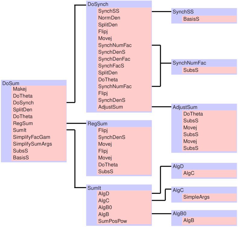
Figure 3.1: Internal structure of the XSummer package

3.2.1 Procedures to be called directly

BasisS
        Express products of $S$-sums into single $S$-sums of higher weight.

ConvStoZ
        Convert $S$-sums into $Z$-sums.

DoSum
        User front-end to the XSummer package. The first parameter denotes the index of the innermost summation, the second is the index of the outermost sum, which should be summed. For example

    #call DoSum(3,1)

would do the sums over $j_{3}$, $j_{2}$, $j_{1}$ in this order.

An overview of the internal structure of DoSum is shown in Fig. 3.1.

3.2.2 Internal procedures

AdjustSum
        Adjusts the sum boundaries. The argument specifies the index $i$ of the sum to be adjusted.

AlgB
        Implementation of the convolution algorithm (type B) to perform sums of the type $$\sum\limits_{i=1}^{n-1}{x_{1}^{i}\over i^{m_{1}}}S(i;m_{2},...,m_{k};x_{2},...,x_{k}){(x^{\prime}_{1})^{n-i}\over(n-i)^{m^{\prime}_{1}}}S(n-i;m^{\prime}_{2},...,m^{\prime}_{l};x^{\prime}_{2},...,x^{\prime}_{l})\,,$$ for any (integer) values of $m_{i},m_{i}^{\prime}$ and $m_{1}>0$. The argument specifies the index $i$ of the sum to be done. The special case $m_{1}=0$ is handled in AlgB0.

AlgB0
        Special case of the convolution algorithm (type B), for details see AlgB.

AlgC
        Implementation of the conjugation algorithm (type C) to perform sums of the form $\displaystyle\sum\limits_{i=1}^{n}\,\left(\begin{array}[]{c}n\\ i\end{array}\right)\,(-1)^{i}{x_{1}^{i}\over i^{m_{1}}}S(i;m_{2},...,m_{k};x_{2},...,x_{k})\,$ for any (integer) values of $m_{i}$ and $m_{1}>0$. The argument specifies the index $i$ of the sum to be done. The special case $m_{1}=0$ is treated in AlgC0.

AlgC0
        Special case of the conjugation algorithm (type C), for details see AlgC.

AlgD
        Implementation of the binomial convolution algorithm (type D) to perform sums of the form $\displaystyle\sum\limits_{i=1}^{n-1}\,\left(\begin{array}[]{c}n\\ i\end{array}\right)\,(-1)^{i}{x_{1}^{i}\over i^{m_{1}}}S(i;m_{2},...,m_{k};x_{2},...,x_{k})$ $\displaystyle\hskip 28.45274pt\times{(x^{\prime}_{1})^{n-i}\over(n-i)^{m^{\prime}_{1}}}S(n-i;m^{\prime}_{2},...,m^{\prime}_{l};x^{\prime}_{2},...,x^{\prime}_{l})\,$ for any (integer) values of $m_{i},m_{i}^{\prime}\geq 0$ and $m_{1}>0$. The argument specifies the index $i$ of the sum to be done. The special case $m_{1}=0$ is treated in AlgD0.

AlgD0
        Special case of the binomial convolution algorithm (type D); see AlgD.

DoSynch
        Procedure to synchronize the arguments of num, den, fac, invfac and S. The argument specifies the index $i$ of the sum to be adjusted. Start with synchronizing products of S functions, then do the combinations 1. $j_{i}$ and fac, invfac 2. den and S 3. den and fac, invfac 4. S and fac, invfac. Finally summation boundaries are synchronized.

DoTheta
        Simplifies combinations of theta, delta, deltap and sum functions, defined for each sum over $j_{i}$. The argument specifies the index $i$ of the sum to be adjusted (argument $i=0$ implies no sum).

ExpandDen
        Expands den function in small parameter ep, i.e. $1/(a+b\epsilon)$ in terms of $\epsilon$. If the argument provided to ExpandDen is 0 then denominators with integer values of $a$ are expanded. If the argument is 1, we expand for symbolic $a$.

ExpandGam
        Expands Gamma and InvGamma functions in the small parameter ep, i.e. $\Gamma(i+a\epsilon)$ and $1/\Gamma(i+a\epsilon)$ in $\epsilon$, where $i$ and $a$ take integer values. The argument specifies the number of the highest sum in the expression. We choose the $\overline{\mbox{MS}}$-scheme, i.e. $\exp(-\gamma_{E}a\epsilon)=1$, where $\gamma_{E}$ is Euler’s constant.

Flipj
        Reverses the direction of summation. The argument specifies the index $i$ of the sum to be flipped.

Makej
        Creates the dressed objects, for example the pow function pow(x,j3) is converted to pow3(x,j3). The argument specifies the summation index to be treated.

Movej
        Makes a translation of $j_{i}+n$ $\to$ $j_{i}$. The first argument specifies which index $i$ of the summation variable which should be used. The shift is determined by the argument of the function specified by the second argument passed to Movej.

NormDen
        Converts den functions to normal form, i.e. fixes the sign of the summation index appearing in the denominator. The argument specifies the highest summation index $i$ to be treated. The hierarchy is such that $j_{1}$ is more important than $j_{2}$ etc.

NormalizeGam
        Normalizes products of Gamma and InvGamma functions.

RegSum
        Performs final regularization of a sum. The argument specifies the index $i$ of the sum to be regularized.

SimpleArgs
        Applies some trivial simplifications. If the argument passed to SimpleArgs is 0 these simplifications are applied to the prefactors multiplying functions. If the argument passed is C the simplifications are applied to the arguments of S and pow functions.

Simplify
        Calls different simplification and normalization routines to simplify or normalize the expresssions.

SimplifyFacGam
        Procedure to simplify products of fac, invfac and Gamma, InvGamma functions.

SimplifySumArgs
        Procedure to simplify polynomials in arguments of S functions. This procedure is user accessible and should be edited if optimization is needed.

SplitDen
        Partial fractioning of products of denominators involving the summation variable $j_{i}$, where $i$ is the argument passed to SplitDen. This routine is optimized for higher powers of the denominators and uses the sum formula rather than repeated splitting of pairs.

SubsS
        Evaluates S functions with a numerical last argument into polynomials in the variables (if possible, with numerical values). For argument $i=0$ only numerical values are realized; for $i=1$ the procedure also expands polynomials. S functions with symbolic last argument are untouched, of course.

SumIt
        Calls the various procedures for summation algorithms. The argument specifies the index $i$ of the sum to be done.

SumPosPow
        Sums positive (or zero) powers of $j_{i}$ possibly in combination with one S or pow function. The argument specifies the index $i$ of the sum to be done.

SynchDenFac
        Synchronizes combinations of den and fac, invfac functions, i.e. factorials and denominators. The argument specifies the associated summation index $i$.

SynchDenS
        Synchronizes combinations of den and S functions, i.e. denominators and $S$-sums. The argument specifies the associated summation index $i$.

SynchFacS
        Synchronizes combinations of S and fac, invfac functions, i.e. factorials and $S$-sums. The argument specifies the associated summation index $i$.

SynchNumFac
        Synchronizes combinations of (positive) powers of $j_{i}$ and fac, invfac functions. The argument specifies the associated summation index $i$.

SynchSS
        Synchronizes products of $S$-sums. The argument specifies the associated summation index $i$.

As discussed in Section 2 the $S$-sums can be treated as generalization of the harmonic sums investigated in Refs. [1, 9, 18]. It is therefore evident that some of the procedures presented here are similar to those in the Summer package [9] written by J.A.M. Vermaseren. In particular the procedures AdjustSum, BasisS, DoSynch, DoTheta, Flipj, Makej, SubsS, SynchDenFac and SynchSS are adapted versions of similar procedures in Summer.

3.2.3 Harmonic sums in infinity

A special class of sums, occurring as a result of the summation algorithms, are harmonic sums in infinity. These are related to multiple zeta values [2], which for a given weight are reducible to a small set of transcendental numbers using, for example, the algebraic properties in Eq. (2.6).

Together with the XSummer package, we provide the tables of harmonic sums in infinity (limited to weight six). These procedures are called tables, table1, … , table6 and the corresponding files are directly extracted from the Summer package [9]. This facilitates interfacing with routines of the current package.

Let us also note that the reduction of multiple zeta values of a given weight to some irreducible set of constants is currently an active field of mathematical research. Currently, downloads of tables up to weight nine in Form [23] or Maple format [24] are publicly available and extensions are known up to weight 16 [25, 26].

4 Examples

Along with the distribution of the XSummer  package, we provide also a number of non-trivial examples. These examples can either be run with the help of the shell script TestIt in a standard Linux/Unix environment or with the help of TestItXP.bat under the Microsoft Windows XP operating system. (For either of the scripts the user might have to make small adaptations, though.)

The respective script executes the Form  files Examples.frm and DoIntegrals.frm (discussed in detail below) and performs a check on the output of the former computations against tabulated results with the help of the file CheckResults.frm. In this way, the user can verify the correctness of the installation of the XSummer  package. At the same time, the examples are meant to illustrate the usage of sums with the XSummer  package. In particular, we want to clarify the conventions for the input to the procedures of Section 3.

We provide in the file Examples.frm a number of (generalized) hypergeometric functions from the original Ref. [4],

       hypergeom2F1(a*ep,b*ep,1-c*ep,x1)
       hypergeom2F1(1,-ep,1-ep,x1)
       hypergeom3F2(-2*ep,-2*ep,1-ep,1-2*ep,1-2*ep,x1)
       appel2(1,1,ep,1+ep,1-ep,x1,x2)

where the coefficients of Laurent series in $\epsilon$ are calculated up to a given order in terms of multiple polylogarithms. The first example hypergeom2F1(a*ep,b*ep,1-c*ep,x1) was actually given in Eq. (1.1). In Examples.frm it is realized by the following set of substitutions:

id hypergeom2F1(a?,b?,c?,x1?) = sum1(j1,0,inf) *
      Po(j1+a,a)*Po(j1+b,b)*InvPo(j1+c,c)*invfac(j1)* pow(x1,j1);

id    Po(x1?,x2?) = Gamma(x1)*InvGamma(x2);
id InvPo(x1?,x2?) = Gamma(x2)*InvGamma(x1);

Here Po(x1,x2) and InvPo(x1,x2) denote the Pochhammer symbols, see Eq. (1.1).

Next, the file DoIntegrals.frm calculates certain one- and two-loop Feynman integrals used in a complete calculation of higher-order perturbative corrections in Quantum Chromodynamics [7]. To that end, integrals of various topologies had to be considered. The respective analytical representations in terms of nested sums valid for arbitrary powers of denominators for the so-called C-topology [4], the B-box (one-loop box with one external mass [27]) and one-loop triangles with up to two external masses [28] are all given in the procedure Int2Sum. The input to DoIntegrals.frm, i.e. the information on the topology and on the particular values for the powers of denominators, is passed on by preprocessor variables in Form. The explicit lists of all inputs are contained in SelectIntegral.

In the actual calculation, we choose dimensional regularization [29, 30, 31, 32] with $D=4-2\epsilon$ and the modified [33] minimal subtraction [34] scheme for all loop integrals in this section. For illustration we give here the explicit series representation as we use it in Int2Sum for the one-loop triangle with two external masses $\mbox{Tri}(m,\nu_{1},\nu_{2},\nu_{3};x_{1})$. It is defined by

$$\mbox{Tri}(m,\nu_{1},\nu_{2},\nu_{3};x_{1})=\left(-s_{12}\right)^{-m+\epsilon+\nu_{123}}\int\frac{d^{D}k_{1}}{i\pi^{D/2}}\frac{1}{\left(-k_{1}^{2}\right)^{\nu_{1}}}\frac{1}{\left(-k_{2}^{2}\right)^{\nu_{2}}}\frac{1}{\left(-k_{3}^{2}\right)^{\nu_{3}}}\,$$ (4.1)

and, in the following, we use the short-hand notation $\nu_{ij}=\nu_{i}+\nu_{j}$ for sums of powers of propagators. We have $k_{2}=k_{1}-p_{1}$, $k_{3}=k_{2}-p_{2}$, and we define the quantities

$$s_{12}=\left(p_{1}+p_{2}\right)^{2}\,,\quad\quad\quad\quad x=\frac{p_{1}^{2}}{s_{12}}\,.$$ (4.2)

Equation (4.1) can be written as a combination of hypergeometric functions ${}_{2}F_{1}$. The series representation for this integral with $|x|\leq 1$ is given by

$$\mbox{Tri}(m,\nu_{1},\nu_{2},\nu_{3};x)\,=\,\frac{\Gamma(\epsilon-m+\nu_{23})\Gamma(1-\epsilon+m-\nu_{23})\Gamma(m-\epsilon-\nu_{13})}{\Gamma(\nu_{1})\Gamma(\nu_{2})\Gamma(\nu_{3})\Gamma(2m-2\epsilon-\nu_{123})}$$

$$\hskip 14.22636pt\times\sum\limits_{i=0}^{\infty}\frac{x^{i}}{i!}\bigg{[}x^{m-\epsilon-\nu_{23}}\frac{\Gamma(i_{1}+\nu_{1})\Gamma(i_{1}-\epsilon+m-\nu_{2})}{\Gamma(i_{1}+1+m-\epsilon-\nu_{23})}$$

$$\hskip 71.13188pt-\frac{\Gamma(i_{1}+\nu_{3})\Gamma(i_{1}-m+\epsilon+\nu_{123})}{\Gamma(i_{1}+1-m+\epsilon+\nu_{23})}\bigg{]}\,.$$ (4.3)

Equation (4) is implemented in the procedure Int2Sum and prepared for the input to the XSummer  package with a set of substitutions similar to those briefly discussed above for the ${}_{2}F_{1}$ hypergeometric function.

Now, with the examples at hand, we would like to discuss the efficiency of the implementation of the XSummer  package in Form. As already mentioned above, certainly one major disadvantage in using Form is the lack of internal algorithms for polynomial algebra. As a consequence, we cannot easily bring rational functions of polynomials to a normal form. For that purpose, we would need operations such as factorization, polynomial division or combinations thereof as used for instance in partial fractioning. In applications of the algorithms A–D to sums with multiple scales, this problem becomes apparent when trying to normalize the arguments of the $S$-sums. In particular, the recursions of the conjugation algorithm (type C) are sensitive to this issue. Here, efficient simplifications of polynomials can have a significant impact on the execution time for a given sum.

Since no really elegant way for simplifying polynomials exists within Form, we have provided a case-by-case solution. Inside the procedure AlgC we do have the (user-accessible) procedure SimpleArgs (described in the previous section). There, depending on the scales involved, appropriate substitutions for tuning or optimizations should be added. Then, we do have the procedure CustomizeDen. It uses partial fractioning and normalizes the ubiquitous denominators to standard factors. In a similar spirit, we also use the procedure ParFrac, which brings two-scale polynomials to normal form in DoIntegrals.frm by means of partial fractioning at the end of the calculation.

Another more generic approach to this problem, which the experienced user might consider, is the following. Form  provides the preprocessor statements #system and #pipe, which invoke a call to the operating system. This provides the opportunity to realize a link to external programs, in particular to computer algebra systems such as Maple  or Mathematica  along with their functionalities in polynomial algebra. However, both the detailed description and the implementation of these features is beyond the scope of the present work.

Finally, we would like to give some information on the use of computer resources. Typically, the execution times and the use of memory or disk space depend very much on the problem under consideration. As a general rule, the expression size and therefore the execution time correlate strongly with the depth of the Laurent expansion in $\epsilon$. In the examples, we can control this with the preprocessor variable EXPANDEP. This effectively cuts the series expansion in $\epsilon$ at the specified power. Note that for every individual term the series is cut to the specified order. If additional poles are present it might thus be necessary to expand individual terms to higher order to make sure that no terms are lost. For safeguard, we added a function order, which shows the effect of the truncation. Of course, the run time is also correlated with the number of nested sums. In practical applications it might be advantageous to start with a low value for EXPANDEP and increase it until the final result has the desired order. In addition to this, in practical applications, some tuning may be needed for new large problems, particularly in bringing polynomials to normal form.

Let us close this section with a few remarks about the runtime performance. To give the interested user a hint on how long the presented examples will take, we measured the runtime on a standard PC. In particular, the machine we used was equipped with a 3 GHz P4 (hyperthreading support) with 512 MB of RAM. The considered problems fit completely into the RAM so that the hard-drive speed plays only a marginal rôle. The results are shown in Table 2, where we averaged always over 10 independent runs.

		DoIntegrals.frm
Form 3.1 executable	Examples.frm	CTOPO	BBOX	TRIMASS
gcc, 15-jul-2005	7.9s	20.9s	119.3s	19s
icc, 24-jan-2003	7.5s	19.9s	108.2s	17.4s
gcc, 17-oct-02	8.7s	24.5s	181.3s	27.6s

Table 2: Runtimes of the examples under Linux for different Form versions.

The different Form versions used are available at http://www.nikhef.nl/~form. We also tried a preliminary version of a native Microsoft Windows XP Form executable. The runtimes are very similar to those obtained with the icc-compiled Form executable and the new gcc version. The difference of 5% might be due to the fact that on Windows XP the total time was measured and not only the user time.

In applications more involved than the examples shown here, the user is advised to make a detailed analysis on the actual depth of the expansion in $\epsilon$ needed and on the particular structure of the polynomials. Furthermore the user should provide additional routines to simplify the symbolic arguments of $S$-sums.

5 Conclusion

Symbolic summation has advanced to an important method, e.g. in perturbative quantum field theory, and significant progress has been made during the past years. In the present work, we have provided an implementation in Form of algorithms suitable for the expansion of transcendental functions in a small parameter around integer values, such that the resulting (generalized) hypergeometric series can be expressed in closed form in multiple polylogarithms.

As examples, we have discussed various applications in quantum field theory, particularly in the calculation of Feynman diagrams at higher orders in perturbation theory. In this context, the XSummer package has been used in perturbative calculations extensively and we believe it may be useful for a larger community. We have chosen Form for the implementation, because it is a fast and efficient computer algebra system and because of its capability to handle large expressions. For convenience of the user, we provide along with XSummer a set of sample calculations. These illustrate the use of the program. An extension of the present implementation to cover also algorithms for generalized sums from expansions around rational numbers (see e.g. [35]) will be the subject of a future publication.

Note added

Very recently, Ref. [36] appeared, which addresses the problem of expanding hypergeometric functions ${}_{J}F_{J-1}$ around integer parameters to arbitrary order. It provides an implementation in Mathematica of the algorithms (2.10), (2.1), i.e. type A and B of the original Ref. [4]. Thus, it is capable of performing some expansions already discussed in Ref. [4] and discussed also in the present Letter, for instance Eq. (1.1).

Acknowledgements

We would like to thank J.A.M Vermaseren for his kind permission to use some files of the Summer  package [9] in the current distribution. The work of S.M. has been supported in part by the Helmholtz Gemeinschaft under contract VH-NG-105 and by the Deutsche Forschungsgemeinschaft in Sonderforschungsbereich/Transregio 9.

References

- [1] L. Euler, Novi Comm. Acad. Sci. Petropol. 20 (1775) 140.
- [2] M.E. Hoffman, http://www.usna.edu/Users/math/meh/biblio.html.
-
[3]
M. Petkovsek, H. Wilf and D. Zeilberger,
http://www.cis.upenn.edu/~wilf/AeqB.html, (1997). - [4] S. Moch, P. Uwer and S. Weinzierl, J. Math. Phys. 43 (2002) 3363, hep-ph/0110083.
- [5] J.A.M. Vermaseren, math-ph/0010025, (2000).
- [6] J.A.M. Vermaseren, Nucl. Phys. Proc. Suppl. 116 (2003) 343, hep-ph/0211297.
- [7] S. Moch, P. Uwer and S. Weinzierl, Phys. Rev. D66 (2002) 114001, hep-ph/0207043.
- [8] L. Lewin, Polylogarithms and Associated Functions (North Holland, New York, 1981).
- [9] J.A.M. Vermaseren, Int. J. Mod. Phys. A14 (1999) 2037, hep-ph/9806280.
- [10] S. Moch, J.A.M. Vermaseren and A. Vogt, Nucl. Phys. B688 (2004) 101, hep-ph/0403192.
- [11] A. Vogt, S. Moch and J.A.M. Vermaseren, Nucl. Phys. B691 (2004) 129, hep-ph/0404111.
- [12] J.A.M. Vermaseren, A. Vogt and S. Moch, hep-ph/0504242, (2005).
- [13] C. Bauer, A. Frink and R. Kreckel, cs/0004015, (2000).
- [14] S. Weinzierl, Comput. Phys. Commun. 145 (2002) 357, math-ph/0201011.
-
[15]
A.B. Goncharov,
Math. Res. Lett. 5 (1998) 497,
(available at http://www.math.uiuc.edu/K-theory/0297). - [16] J.M. Borwein et al., math.CA/9910045.
- [17] E. Remiddi and J.A.M. Vermaseren, Int. J. Mod. Phys. A15 (2000) 725, hep-ph/9905237.
- [18] J. Blümlein, Comput. Phys. Commun. 159 (2004) 19, hep-ph/0311046.
- [19] M.E. Hoffman, J. Algebra 194 (1997) 477.
- [20] M.E. Hoffman, math.QA/0406589.
-
[21]
A. Erdélyi et al.,
Higher Transcendental Functions, Vol. I
(McGraw Hill, New York, 1953). - [22] R.L. Graham, D.E. Knuth and O. Patashnik, Concrete Mathematics (Addison-Wesley, 1994).
- [23] J. Vermaseren, http://www.nikhef.nl/~form/FORMdistribution/packages/summer/index.html.
- [24] M. Petitot, http://www.lifl.fr/~petitot/publis/mzv.tar.
- [25] M. Petitot, private communication.
- [26] J. Vermaseren, http://www.nikhef.nl/~t68/FORMapplications/t1-5.ps.
- [27] C. Anastasiou, E.W.N. Glover and C. Oleari, Nucl. Phys. B565 (2000) 445, hep-ph/9907523.
- [28] C. Anastasiou, E.W.N. Glover and C. Oleari, Nucl. Phys. B572 (2000) 307, hep-ph/9907494.
- [29] G. ’t Hooft and M. Veltman, Nucl. Phys. B44 (1972) 189.
- [30] C.G. Bollini and J.J. Giambiagi, Nuovo Cim. 12B (1972) 20.
- [31] J.F. Ashmore, Lett. Nuovo Cim. 4 (1972) 289.
- [32] G.M. Cicuta and E. Montaldi, Nuovo Cim. Lett. 4 (1972) 329.
- [33] W.A. Bardeen et al., Phys. Rev. D18 (1978) 3998.
- [34] G. ’t Hooft, Nucl. Phys. B61 (1973) 455.
- [35] S. Weinzierl, J. Math. Phys. 45 (2004) 2656, hep-ph/0402131.
- [36] T. Huber and D. Maitre, hep-ph/0507094.