Explicit invariant measures for products of random matrices

Abstract.

We construct explicit invariant measures for a family of infinite products of random, independent, identically-distributed elements of $\text{SL}(2,{\mathbb{C}})$. The matrices in the product are such that one entry is gamma-distributed along a ray in the complex plane. When the ray is the positive real axis, the products are those associated with a continued fraction studied by Letac & Seshadri [Z. Wahr. Verw. Geb. 62 (1983) 485-489], who showed that the distribution of the continued fraction is a generalised inverse Gaussian. We extend this result by finding the distribution for an arbitrary ray in the complex right-half plane, and thus compute the corresponding Lyapunov exponent explicitly. When the ray lies on the imaginary axis, the matrices in the infinite product coincide with the transfer matrices associated with a one-dimensional discrete Schrödinger operator with a random, gamma-distributed potential. Hence, the explicit knowledge of the Lyapunov exponent may be used to estimate the (exponential) rate of localisation of the eigenstates.

1. introduction

Let $\{{\mathcal{A}}_{n}\}_{n\in{\mathbb{N}}}$ denote a sequence of independent random matrices identically distributed according to a probability measure $\mu$ on $\text{GL}(2,{\mathbb{R}})$. The problem of determining the asymptotic behaviour of the product

(1.1) $${\mathcal{M}}_{n}:={\mathcal{A}}_{1}{\mathcal{A}}_{2}\cdots{\mathcal{A}}_{n}\quad\text{as $n\rightarrow\infty$},$$

plays a crucial rôle in the theory of products of random matrices and its applications, especially in mathematical physics [6, 7].

The rate of growth of this product can be quantified by its Lyapunov exponent

(1.2) $$\lambda:=\lim_{n\rightarrow\infty}\frac{1}{n}{\mathbb{E}}\left(\ln|{\mathcal{M}}_{n}|\right),$$

where $|\cdot|$ denotes some matrix norm.

The Lyapunov exponent exists whenever ${\mathbb{E}}(\log^{+}|A_{1}|)<\infty$. The Furstenberg–Kesten theorem ([14], [6] p. 11) generalises the classical strong law of large numbers to the case of non-commuting random products and states that

$$\lambda=\lim_{n\rightarrow\infty}\frac{1}{n}\ln|{\mathcal{M}}_{n}|\quad\text{almost surely.}$$

The case of unimodular matrices (i.e. ${\mathcal{A}}_{n}\in\text{SL}(2,{\mathbb{R}})$) is of particular interest. In this case, under the natural additional assumption of noncompactness and strong irreducibility, Furstenberg’s theorem ([13], cf. [6] p. 30), asserts that the Lyapunov exponent is strictly positive. Moreover, there exists a unique, continuous, $\mu$-invariant measure $\nu$ on the projective line $P\left({\mathbb{R}}^{2}\right)$— that is, a measure that is invariant under the projective action of matrices drawn from the distribution $\mu$ (cf. [6] p. 30).

The calculation of the Lyapunov exponent involves this $\mu$-invariant measure, but there are remarkably few non-trivial cases where $\nu$ has been found explicitly; three well-known examples will be discussed presently (others are given in [9]) . The prominent feature shared by these examples is that the invariant measure is found by considering a random continued fraction derived from the projective action of the relevant matrix ensemble.

The first example dates back to Dyson’s work on the disordered chain problem.

Example 1 (Dyson [12]).

The disordered chain is modeled by a system of harmonic oscillators coupled by linear forces. A physical realisation is obtained by considering a sequence of $N$ particles joined by elastic springs obeying Hooke’s law. Denote the mass and the displacement of the $n$th particle from its equilibrium position by $m_{n}$ and $x_{n}$ respectively, and let $k_{n}$ be the elastic modulus of the spring between the $n$th and $(n+1)$th particle. Then the equation of motion takes the form

$$m_{n}\,\ddot{x}_{n}=k_{n}(x_{n+1}-x_{n})+k_{n-1}(x_{n-1}-x_{n}),\quad 1\leq n\leq N\,.$$

By introducing additional variables, it is straightforward to express this as the first-order system

$$\dot{u}_{n}=\sqrt{a_{n}}\,u_{n+1}-\sqrt{a_{n-1}}\,u_{n-1},\quad 1\leq n\leq 2N-1,$$

where

$$a_{2n-1}:=\frac{k_{n}}{m_{n}},\quad a_{2n}:=\frac{k_{n}}{m_{n+1}}\,.$$

In matrix notation,

$$\dot{\mathbf{u}}={\mathcal{J}}{\mathbf{u}},$$

where ${\mathcal{J}}$ is the tridiagonal (Jacobi) matrix

$${\mathcal{J}}=\begin{pmatrix}0&\sqrt{a_{1}}&0&0&0&\ldots&0\\ -\sqrt{a_{1}}&0&\sqrt{a_{2}}&0&0&\ldots&0\\ 0&-\sqrt{a_{2}}&0&\sqrt{a_{3}}&0&\ldots&0\\ \vdots&&&&&&\vdots\\ 0&0&\ldots&0&-\sqrt{a_{2N-3}}&0&\sqrt{a_{2N-2}}\\ 0&0&\ldots&0&0&-\sqrt{a_{2N-2}}&0\\ \end{pmatrix}\,.$$

Dyson studied the spectral problem for ${\mathcal{J}}$ when the $a_{n}$ are independent, identically distributed random variables. It turns out that the spectral properties of ${\mathcal{J}}$ (e.g. the eigenvalue density function) can be deduced from the so-called characteristic function of the chain

$$\Omega(t):=2\,\int_{0}^{\infty}\,\ln(1+x)\nu_{t}(\text{d}x),$$

where $\nu_{t}$ is the distribution of the random continued fraction

(1.3) $$\cfrac{a_{1}t}{1+\cfrac{a_{2}t}{1+\cfrac{a_{3}t}{1+\cdots}}}\,.$$

To illustrate his approach, Dyson elaborated the particular case where the $a_{n}$ are gamma-distributed, i.e. for every Lebesgue-measurable subset $S$ of ${\mathbb{R}}_{+}$,

$$\text{Pr}\left(a_{n}\in S\right)=\int_{S}\gamma_{p,s}(a)\,\text{d}a,$$

where

(1.4) $$\gamma_{p,s}(a):=\frac{1}{s^{p}\Gamma(p)}\,a^{p-1}\text{e}^{-\frac{a}{s}}\,,\quad a\geq 0;\;p,s>0\,.$$

Then the probability density function of the random continued fraction (1.3) is given explicitly by

$$\nu_{t}(\text{d}x)=C_{p,s,t}\frac{x^{p-1}}{(1+x)^{p}}\exp\left(-\frac{x}{st}\right)\,\text{d}x,$$

where $C_{p,s,t}$ is a normalisation constant.

In terms of products of random matrices, Dyson’s continued fraction (1.3) corresponds to the case where

$${\mathcal{A}}_{n}=\begin{pmatrix}0&a_{n}t\\ 1&1\end{pmatrix}$$

in the product (1.1). The distribution $\nu_{t}$ of the continued fraction is the $\mu$-invariant distribution associated with this product.

One of the present paper’s contribution is the calculation of the distribution of a random continued fraction that arises in another important physical model, namely the discrete Schrödinger equation with a random potential. In this regard, Lloyd’s model (cf. [20], [16], [22]) with a Cauchy-distributed potential in one spatial dimension is possibly the best-known example where the invariant measure and the corresponding Lyapunov exponent have been found explicitly.

Example 2 (Lloyd’s model [6], p. 35).

Let $z=x+\text{i}y\in{\mathbb{C}}$ with $y>0$ and denote by $C_{z}$ the distribution of the random variable $x+yc$, where $c$ is Cauchy-distributed, i.e

$$\text{Pr}\left(c\in S\right)=\frac{1}{\pi}\int_{S}\frac{\text{d}t}{1+t^{2}}$$

for every Lebesgue-measurable subset $S$ of ${\mathbb{R}}$. Set

$${\mathcal{A}}_{n}:=\begin{pmatrix}a_{n}&-1\\ 1&0\end{pmatrix}\in\text{SL}(2,{\mathbb{R}}),$$

where the $a_{n}$ are independent and $C_{z}$-distributed. The invariant measure $\nu$ is then given by the distribution $C_{u}$, where $u$ and $z$ are related by $z=u+1/u$. It follows easily that

$$\lambda=\ln|u|\,.$$

We end our brief survey with an example that, once again, involves a continued fraction with gamma-distributed elements; the resulting invariant distribution is a so-called generalised inverse Gaussian distribution.

Example 3 (The generalised inverse Gaussian distribution [6], pp. 170-171).

Set

(1.5) $${\mathcal{A}}_{n}:=\begin{pmatrix}0&1\\ 1&a_{n}\end{pmatrix},$$

where the $a_{n}$ are independent, gamma-distributed random variables with parameters $p$ and $s$. It was shown by Letac and Seshadri [18] that the probability density function of the invariant measure $\nu$ is then

(1.6) $$f_{0}(x):=\frac{1}{2K_{p}(2/s)}\,x^{-p-1}\exp\left[-\frac{1}{s}\left(x+\frac{1}{x}\right)\right]\,,\quad x\geq 0,$$

where $K_{p}$ is the modified Bessel function of order $p$. As we will show below, the Lyapunov exponent can be expressed in terms of modified Bessel functions. The details can be found in Section 6. See also [19] and [5] for some generalisations of this example.

In the papers that form the basis of Examples 1 and 3, the authors were concerned — not with products of random matrices— but rather with the problem of determining the distribution of a continued fraction with random coefficients. We have already mentioned Dyson’s continued fraction (1.3). The continued fraction studied by Letac & Seshadri is of the form

(1.7) $$X=\cfrac{1}{a_{1}+\cfrac{1}{a_{2}+\cfrac{1}{a_{3}+\cdots}}}\,,$$

where, as in Dyson’s case, the $a_{n}$ are independent and gamma-distributed.

In this paper, we generalise this example to the case where the elements take values along a ray in the complex plane. Hence, from now on, unless explicitly stated otherwise, we consider matrices in $\text{GL}(2,{\mathbb{C}})$.

1.1. Main results

Fix a constant

$$\alpha\in(-\pi/2,\pi/2)$$

and consider the one-parameter family of complex matrices of the form

(1.8) $${\mathcal{A}}_{n}(\alpha):=\begin{pmatrix}0&1\\ 1&a_{n}\text{e}^{\text{i}\alpha}\end{pmatrix},$$

where the $a_{n}$ are, again, independent gamma-distributed random variables.

The corresponding random continued fraction is

(1.9) $$Z=\cfrac{1}{a_{1}\text{e}^{\text{i}\alpha}+\cfrac{1}{a_{2}\text{e}^{\text{i}\alpha}+\cfrac{1}{a_{3}\text{e}^{\text{i}\alpha}+\cdots}}}\,.$$

The random variable $Z$ takes values in the cone

(1.10) $$S_{\alpha}=\left\{z\in{\mathbb{C}}:\;|\arg z|\leq|\alpha|\right\}\,.$$

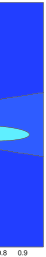
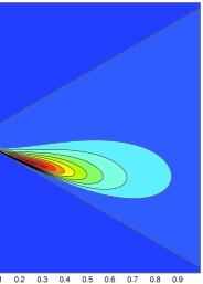
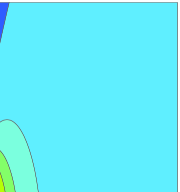
Figure 1. The probability density function of $Z$ for $p=s=1$ and four different values of $\alpha$: (a) $\pi/20$, (b) $\pi/6$, (c) $\pi/3$ and (d) $9\pi/20$. Blue and red correspond to low and high probability respectively. For values of $\alpha$ close to $0$ (resp. $\pi/2$) the density is localised near the positive real half-line (resp. the imaginary axis), see Theorem 2 and §5.

Our main contribution is an explicit formula for the distribution of $Z$ or, equivalently, for the $\mu$-invariant measure $\nu$ associated with the infinite product of the random matrices (1.8).

Theorem 1.

Let $0<|\alpha|<\pi/2$. Suppose that the $a_{n}$ are independent, gamma-distributed random variables with parameters $p,s>0$, and write $z=r\text{\em e}^{\text{\em i}\theta}$. Then the probability density function of $Z$— equivalently, that of the $\mu$-invariant measure $\nu$— is supported on $S_{\alpha}$ and given by

(1.11) $$f_{\alpha}(z)=\frac{\sin(2|\alpha|)}{\left|2K_{p}\left(2\text{e}^{\text{\em i}\alpha}/s\right)\right|^{2}}\frac{1}{r^{2}\sin^{2}(\alpha+\theta)}\left[\frac{\sin(\alpha-\theta)}{\sin(\alpha+\theta)}\right]^{p-1}\\ \times\exp\left\{-\frac{\sin(2\alpha)}{s}\left[\frac{1}{r\sin(\alpha-\theta)}+\frac{r}{\sin(\alpha+\theta)}\right]\right\}\,.$$

In particular, the density is a smooth function that decays exponentially fast at infinity in every direction contained in the cone $S_{\alpha}$.

Plots of the probability density function $f_{\alpha}$ for $p=s=1$ and various values of $\alpha$ are shown in Figure 1.

In Section 6, we use the above result to calculate the corresponding Lyapunov exponent and express it in terms of the logarithmic derivative of the modified Bessel function, namely (see Theorem 4)

$$\lambda_{p,s}(\alpha)=\operatorname{Re}\frac{\partial_{p}K_{p}\left(\frac{2}{s}e^{i\alpha}\right)}{K_{p}\left(\frac{2}{s}e^{i\alpha}\right)}.$$

By considering the weak limit in (1.11) as $\alpha\rightarrow 0$, we recover the distribution found originally by Letac and Seshadri (see Section 5).

The behaviour of the random variable $Z$ as $|\alpha|\rightarrow\pi/2-$ is particularly interesting. Figure 2 shows plots of the probability density function of $\arg Z$ for various values of $\alpha$ when $p=s=1$. As $|\alpha|$ approaches $\pi/2$, the support of the measure $\nu$ becomes concentrated on the imaginary axis.

Figure 2. The probability density function of $\arg Z$ for $p=s=1$ and various values of $\alpha$.

The weak limit as $|\alpha|\rightarrow\pi/2-$ leads to our second result:

Theorem 2.

Let $|\alpha|=\pi/2$. Suppose that the $a_{n}$ are independent and gamma-distributed, with parameters $p,s>0$, and write $z=x+\text{\em i}y$. Then, the probability density function of $Z$— equivalently, that of the $\mu$-invariant distribution $\nu$— is given by

(1.12) $$f_{\pm\pi/2}(z)=\frac{\delta(x)}{\pi^{2}\left[J_{p}^{2}(2/s)+Y_{p}^{2}(2/s)\right]}\,\frac{1}{y^{p+1}}\exp\left[\pm\frac{1}{s}\left(\frac{1}{y}-y\right)\right]\\ \times\int_{c(y)}^{y}\exp\left[\mp\frac{1}{s}\left(\frac{1}{t}-t\right)\right]\,t^{p-1}\,\text{d}t\,,$$

where

$$c(y)=\begin{cases}-\infty&\text{if $y<0$}\\ 0&\text{if $y>0$}\end{cases}$$

and $\delta$ is the Dirac delta. In particular, $\nu$ is supported on the imaginary axis, where the density decays algebraically (like $1/y^{2}$) at $\pm\infty$.

Plots of $f_{\pi/2}(\text{i}y)$ for various values of $p$ and $s$ are shown in Figure 3. For comparison, the figure includes a plot of the Cauchy probability density function. We shall see in §4 that, for $\alpha=\pm\pi/2$ and $s$ small, $Z$ is approximately Cauchy-distributed along the imaginary axis.

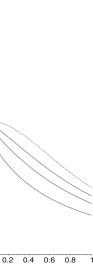
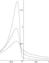
Figure 3. The probability density function $f_{\pi/2}$ for $x=0$ and various values of the parameters $s$ and $p$: (a) $p=1$; (b) $s=1$. The dashed curve in (a) corresponds to the Cauchy probability density function $\frac{1}{\pi}\frac{1}{1+y^{2}}$.

Next, we discuss some interesting applications of these results.

1.2. Random Schrödinger operators

In 1958, P. W. Anderson [2] postulated that the spectra of Schrödinger operators with random potentials should exhibit a tendency towards a dense pure point spectrum with bound eigenstates. When the eigenstates decay exponentially fast, one speaks of strong or exponential localisation. This type of localisation has been proved for one-dimensional systems; cf. [7], Chap. VIII. Higher-dimensional systems will not be considered here; we refer the reader to [7] for a discussion of that case.

In order to make the connection between this general theory and our own results, let us first note that by conjugating the matrices (1.8) for $\alpha=\pi/2$ with a rotation that maps $P({\mathbb{R}}^{2})$ into the imaginary line, we obtain

$$R^{*}{\mathcal{A}}_{n}(\alpha)R=\text{i}\begin{pmatrix}0&-1\\ 1&a_{n}\end{pmatrix},\qquad\text{ where }\quad R=\begin{pmatrix}\text{i}&0\\ 0&1\end{pmatrix}.$$

Thus the corresponding random matrices reduce in this limiting case to the transfer matrices for the discrete stationary one-dimensional Schrödinger equation

(1.13) $$(-\Delta+V)\,y=E\,y\,$$

with $y=\{y_{n}\}_{n\in\mathbb{Z}}$, $(\Delta y)_{n}=y_{n+1}-2y_{n}+y_{n-1}$ (tight-binding, nearest-neighbour laplacian), $(V\,y)_{n}=a_{n}y_{n}$ (independent identically distributed random potential) and energy level $E=2$ (cf. [6], p. 187).

It is readily seen that the above equation can be rewritten in the form

$$\begin{pmatrix}y_{n}&y_{n+1}\end{pmatrix}=\begin{pmatrix}y_{n-1}&y_{n}\end{pmatrix}\begin{pmatrix}0&-1\\ 1&a_{n}\end{pmatrix}=(-\text{i})^{n}\,\begin{pmatrix}y_{0}&y_{1}\end{pmatrix}R^{\ast}{\mathcal{M}}_{n}(\pi/2)R\,.$$

It is well known [17] that the spectrum on $\ell^{2}(\mathbb{Z})$ of the Hamiltonian associated with Equation (1.13), i.e of the operator $H=-\Delta+V$ is given, with probability one, by

(1.14) $$\sigma(H)=\sigma(-\Delta)+\operatorname{supp}(\mu),$$

where $\sigma(-\Delta)=[0,4]$ and $\mu$ denotes the probability measure of the potential.

It has been shown in [8] that, as long as $\mu$ is not concentrated on a single point and possesses some finite moment, the spectrum $\sigma(H)$ is pure-point with probability one. The eigenfunctions are exponentially localised with a rate determined by the value of the Lyapunov exponent (see [7, 6]). Thus is view of our results we have

Proposition 1.1.

Let $H$ be the hamiltonian of the Anderson tight-binding model in dimension 1 with $\gamma_{p,s}$-distributed potential. The exponential localization rate for the energy level

$$E=2\in\sigma(H)=(0,+\infty)$$

is given by

$$\lambda_{s,p}(\pi/2)=\operatorname{Re}\frac{\partial_{p}K_{p}(2i/s)}{K_{p}(2i/s)}.$$

We note that the Lyapunov exponent is a smooth function of the energy level $E$ (cf. [7], Proposition VIII.1.1). Thus, although the above result is not sufficient to give estimates of the decay rate of all the eigenstates, it does yield quantitative information in the close enough neighbourhood of $E=2$, which is almost surely in the bulk of the spectrum.

1.3. Random Stieltjes functions

Another motivation for this work is to study the convergence of Padé approximation for series that are random in some sense [23]. Consider the class of random Stieltjes functions whose continued fraction expansion is

$$F(t)=\cfrac{1}{c_{1}+\cfrac{t}{c_{2}+\cfrac{t}{c_{3}+\cdots}}}\,,\quad t\in{\mathbb{C}}\backslash{\mathbb{R}}_{-},$$

where the $c_{n}$ are independent draws from the gamma distribution with parameters $p$ and $\sigma$. By truncating this continued fraction, we obtain rational approximations of $F$:

(1.15) $$F_{n}(t):=\cfrac{1}{c_{1}+\cfrac{t}{c_{2}+\cdots+\cfrac{t}{c_{n}}}}\,,\quad t\in{\mathbb{C}}\backslash{\mathbb{R}}_{-}\,.$$

It is a well-known fact that the $F_{n}$ are diagonal or near-diagonal Padé approximants of $F$ [3, 4]. Roughly speaking, this means that

$$F(t)-F_{n}(t)=O(t^{n})\quad\text{as $t\rightarrow 0$},$$

and that there is no other rational function— with a numerator and a denominator of lesser degree— with this property. The rate of decay of the error of Padé approximation as $n\rightarrow\infty$, $t$ fixed, is of considerable practical interest.

A simple calculation reveals that the distribution of $\sqrt{t}F(t)$ is precisely that of the random variable $Z$ defined by Equation (1.9) if we take

$$a_{n}=\frac{c_{n}}{\sqrt{|t|}},\quad s=\frac{\sigma}{\sqrt{|t|}}\quad\text{and}\quad\alpha=-\frac{\arg t}{2}\,.$$

The rate of convergence of Padé approximation for a typical realisation of the function $F$ is then given by

$$\frac{\ln\left|F(t)-F_{n}(t)\right|}{n}\xrightarrow[n\rightarrow\infty]{}-2\lambda_{p,\frac{\sigma}{\sqrt{|t|}}}\left(-\frac{\arg t}{2}\right)\quad\text{almost surely.}$$

The proof of this result requires a careful study of the ergodic properties of the Markov chain associated with the continued fraction; a detailed treatment will be given in a separate publication.

The remainder of the paper provides the details of the proofs of these assertions. In the next section, we introduce some notation, elaborate the correspondence between products of $2\times 2$ matrices and continued fractions, and derive an integral equation for the unknown probability density function of $Z$. In §3, we deduce a partial differential equation, and solve it. The case $\alpha=\pm\pi/2$ is treated in §4 and, in §5, we show that the singular measure obtained in this case is a weak limit of that found earlier. Finally, §6 is concerned with the explicit calculation of the Lyapunov exponent.

2. Preliminaries

The correspondence between continued fractions and products of $2\times 2$ matrices is well-known (see for instance [6], Part A, §VI.5), but since it forms the basis of our approach, it is desirable to elaborate it here. The starting point is the observation that any linear fractional transformation

$${\mathcal{F}}(z)=\frac{a_{11}z+a_{12}}{a_{21}z+a_{22}}$$

corresponds to the action of a matrix

(2.1) $${\mathcal{A}}=\begin{pmatrix}a_{11}&a_{12}\\ a_{21}&a_{22}\end{pmatrix}$$

on a complex or real projective line $P({\mathbb{C}}^{2})$. Indeed, denoting by

$${\mathbf{z}}=\begin{pmatrix}z_{1}\\ z_{2}\end{pmatrix}$$

any nonzero vector in ${\mathbb{C}}^{2}$ and defining its projection by

$$\Pi{\mathbf{z}}=\begin{cases}\frac{z_{1}}{z_{2}}&\text{if $z_{2}\not=0$}\\ \infty&\text{otherwise}\end{cases},$$

we obtain a natural identification of $P({\mathbb{C}}^{2})$ with $\Pi{\mathbb{C}}^{2}=\overline{{\mathbb{C}}}={\mathbb{C}}\cup\{\infty\}$. The action of ${\mathcal{A}}$ on $P({\mathbb{C}}^{2})$ (denoted by $\cdot$) can then be defined via

(2.2) $${\mathcal{A}}\cdot z=\Pi{\mathcal{A}}\begin{pmatrix}z\\ 1\end{pmatrix}=\frac{a_{11}z+a_{12}}{a_{21}z+a_{22}}={\mathcal{F}}(z)\,.$$

Then, for the choice

(2.3) $${\mathcal{A}}={\mathcal{A}}(\alpha):=\begin{pmatrix}0&1\\ 1&a\text{e}^{\text{i}\alpha}\end{pmatrix},\quad|\alpha|\leq\frac{\pi}{2},$$

we get

(2.4) $${\mathcal{A}}\cdot z=\frac{1}{z+a\text{e}^{\text{i}\alpha}}=:{\mathcal{F}}_{a}(z)\,.$$

It is convenient to extend the notation for the set $S_{\alpha}$, defined by (1.10) for $0<|\alpha|<\pi/2$, to the limiting cases $\alpha=0,\pm\pi/2$. We shall write

$$S_{0}:={\mathbb{R}}_{+}\quad\text{and}\quad S_{-\pi/2}=S_{\pi/2}:=\text{i}{\mathbb{R}}=\{z\in{\mathbb{C}}:|\arg z|=\pi/2\}\,.$$

Then, for every $a\geq 0$,

$${\mathcal{F}}_{a}\left(S_{\alpha}\right)\subseteq S_{\alpha}\,.$$

Now, suppose that $a$ is a positive random variable distributed according to a probability measure $\mu(\text{d}a)$ on ${\mathbb{R}}_{+}$, and let $\hat{Z}_{0}$ be an arbitrary random variable taking values in $S_{\alpha}$. Consider the iteration

(2.5) $$\hat{Z}_{n}={\mathcal{F}}_{a_{n}}\left(\hat{Z}_{n-1}\right),\;n\in{\mathbb{N}},$$

where the $a_{n}$ are independent draws from $\left({\mathbb{R}}_{+},\mu\right)$. Under appropriate conditions on $\mu$ [11], it can be shown that the Markov chain defined by Equation (2.5) has a stationary distribution $\nu(\text{d}z)$ independent of the starting value $\hat{Z}_{0}$. Moreover, the latter distribution coincides with the distribution of the random continued fraction (1.9), which can be constructed by means of the successive applications of the corresponding random matrices

(2.6) $${\mathcal{M}}_{n}(\alpha)\cdot z:={\mathcal{A}}_{1}(\alpha){\mathcal{A}}_{2}(\alpha)\cdots{\mathcal{A}}_{n}(\alpha)\cdot z={\mathcal{F}}_{a_{1}}\circ{\mathcal{F}}_{a_{2}}\circ\cdots\circ{\mathcal{F}}_{a_{n}}(z)\\ \\ =\cfrac{1}{a_{1}\text{e}^{\text{i}\alpha}+\cfrac{1}{a_{2}\text{e}^{\text{i}\alpha}+\cdots+\cfrac{1}{a_{n}\text{e}^{\text{i}\alpha}+z}}}\,.$$

Hence, the $\mu$-invariant measure on the projective line associated with the infinite product of the ${\mathcal{A}}_{n}$ is precisely $\nu(\text{d}z)$.

Let us denote by $\nu_{n}$ the distribution of $\hat{Z}_{n}$. We are only interested in the case where the measures $\nu_{n}(\text{d}z)$ and $\nu(\text{d}z)$ on $S_{\alpha}$ are absolutely continuous with respect to the Lebesgue measure $\text{d}z$; so let $f_{\alpha,n}$ and $f_{\alpha}$ be the probability density functions of $\hat{Z}_{n}$ and $Z$ respectively, i.e.

$$\nu(\text{d}z)=f_{\alpha}(z)\text{d}z\quad\text{and}\quad\nu_{n}(\text{d}z)=f_{\alpha,n}(z)\text{d}z\quad\text{for $z\in S_{\alpha}$}\,.$$

Our aim is to find an explicit formula for $f_{\alpha}$. To this end, we derive a recurrence relation for the $f_{\alpha,n}$ and hence, by taking the limit as $n\rightarrow\infty$, find an integral equation satisfied by $f_{\alpha}$. We shall assume that $f_{\alpha,n}$ and $f_{\alpha}$ are smooth. We introduce the map ${\mathcal{G}}_{a}:S_{\alpha}\rightarrow{\mathbb{K}}:={\mathbb{R}}$, $\text{i}{\mathbb{R}}$ or ${\mathbb{C}}$ defined by

$${\mathcal{G}}_{a}(z)=\frac{1}{z}-a\text{e}^{\text{i}\alpha}\,.$$

Thus, ${\mathcal{G}}_{a}$ is the left inverse of ${\mathcal{F}}_{a}$:

$$\forall\,z\in S_{\alpha},\quad\left({\mathcal{G}}_{a}\circ{\mathcal{F}}_{a}\right)(z)=z\,.$$

On the other hand, for $z\in S_{\alpha}$,

$$\left({\mathcal{F}}_{a}\circ{\mathcal{G}}_{a}\right)(z)=z$$

only if ${\mathcal{G}}_{a}(z)\in S_{\alpha}$.

Let $S$ be a measurable set. We have

(2.7) $$\Pr\left(\hat{Z}_{n}\in S\right)=\int_{{\mathbb{R}}_{+}}\Pr\left(\hat{Z}_{n}\in S\,\left|\right.\,a_{n}=a\right)\,\mu(\text{d}a)\\ =\int_{{\mathbb{R}}_{+}}\Pr\left({\mathcal{F}}_{a}(\hat{Z}_{n-1})\in S\right)\,\mu(\text{d}a)=\int_{{\mathbb{R}}_{+}}\Pr\left(\hat{Z}_{n-1}\in{\mathcal{G}}_{a}(S)\cap S_{\alpha}\right)\,\mu(\text{d}a)\\ =\int_{A}\int_{{\mathcal{G}}_{a}(S)\cap S_{\alpha}}f_{\alpha,{n-1}}(z)\text{d}z\,\mu(\text{d}a)$$

where

$$A:=\left\{a\in{\mathbb{R}}_{+}:\;{\mathcal{G}}_{a}(S)\cap S_{\alpha}\neq\emptyset\right\}\,.$$

For $a\in A$, we have

$$\int_{{\mathcal{G}}_{a}(S)\cap S_{\alpha}}f_{\alpha,n-1}(z)\text{d}z=\int_{{\mathcal{F}}_{a}\left({\mathcal{G}}_{a}(S)\cap S_{\alpha}\right)}f_{\alpha,n-1}\left({\mathcal{G}}_{a}(w)\right)\,{\mathcal{J}}_{a}(w)\,\text{d}w,$$

where ${\mathcal{J}}_{a}$ is the jacobian of the transformation

$$z={\mathcal{G}}_{a}(w)\,.$$

Hence

$$\Pr\left(\hat{Z}_{n}\in S\right)=\int_{A}\int_{{\mathcal{F}}_{a}\left({\mathcal{G}}_{a}(S)\cap S_{\alpha}\right)}f_{\alpha,n-1}\left({\mathcal{G}}_{a}(w)\right)\,{\mathcal{J}}_{a}(w)\,\text{d}w\,\mu(\text{d}a)\,.$$

Now, consider the region

$$R:=\left\{(a,w)\in{\mathbb{R}}_{+}\times S_{\alpha}:\;a\in A\;\;\text{and}\;\;w\in{\mathcal{F}}_{a}\left({\mathcal{G}}_{a}(S)\cap S_{\alpha}\right)\right\}\,.$$

It is readily verified that

$$R=\left\{(a,w)\in{\mathbb{R}}_{+}\times S_{\alpha}:\;w\in S\;\;\text{and}\;\;a\in A(w)\right\},$$

where

(2.8) $$A(z):=\left\{a\in{\mathbb{R}}_{+}:\;{\mathcal{G}}_{a}(z)\in S_{\alpha}\right\}\,.$$

Hence,

$$\Pr\left(\hat{Z}_{n}\in S\right)=\int_{S}\int_{A(w)}f_{\alpha,n-1}\left({\mathcal{G}}_{a}(w)\right)\,{\mathcal{J}}_{a}(w)\,\mu(\text{d}a)\,\text{d}w\,.$$

It follows that

(2.9) $$f_{\alpha,n}(z)=\int_{A(z)}f_{\alpha,n-1}\left({\mathcal{G}}_{a}(z)\right)\,{\mathcal{J}}_{a}(z)\,\mu(\text{d}a)\,.$$

Taking the limit as $n\rightarrow\infty$, we conclude that, if the continued fraction (1.9) has a smooth probability density function $f_{\alpha}$, then $f_{\alpha}$ satisfies the equation

(2.10) $$f_{\alpha}(z)=\int_{A(z)}f_{\alpha}\left({\mathcal{G}}_{a}(z)\right)\,{\mathcal{J}}_{a}(z)\,\mu(\text{d}a)\quad\forall\,z\in S_{\alpha}\,.$$

We shall henceforth assume that

$$\mu(\text{d}a)=\gamma_{p,s}(a)\text{d}a\,.$$

The Lyapunov exponent will be denoted by

(2.11) $$\lambda_{p,s}(\alpha):=\lim_{n\rightarrow\infty}\frac{1}{n}\ln\left|{\mathcal{M}}_{n}(\alpha)\right|\,.$$

Here,

$$\left|{\mathcal{M}}\right|=\sup_{\left|{\mathbf{z}}\right|=1}\left|{\mathcal{M}}{\mathbf{z}}\right|\,,$$

where $|\cdot|$ denotes the standard euclidean norm on ${\mathbb{C}}^{2}$. We can express the Lyapunov exponent in terms of the measure $\nu$ as follows

(2.12) $$\lambda_{p,s}(\alpha)=-\int_{S_{\alpha}}\ln|z|\,\nu(\text{d}z)=-\int_{S_{\alpha}}\ln|z|\,f_{\alpha}(z)\text{d}z\,.$$

A proof is given Appendix C.

Remark 2.1.

An equivalent way of presenting our results is to work with the reciprocal of the continued fraction (1.9), i.e.

(2.13) $$a_{1}\text{e}^{\text{i}\alpha}+\cfrac{1}{a_{2}\text{e}^{\text{i}\alpha}+\cfrac{1}{a_{3}\text{e}^{\text{i}\alpha}+\cdots}}\,.$$

The corresponding linear fractional transformation is

$$z\mapsto a\text{e}^{\text{i}\alpha}+1/z$$

and so the matrices in the product (1.1) are of the form

(2.14) $$\begin{pmatrix}a\text{e}^{\text{i}\alpha}&1\\ 1&0\end{pmatrix}\,.$$

In particular, when $\alpha=\pi/2$, we have

$$(-\text{i})\,R^{\ast}\begin{pmatrix}a\text{e}^{\text{i}\alpha}&1\\ 1&0\end{pmatrix}R=\begin{pmatrix}a_{n}&-1\\ 1&0\end{pmatrix}\,.$$

Readers familiar with the application of the theory of products of random matrices to the spectral theory of Schrödinger operators will easily recognize the Schrödinger transfer matrix on the right-hand side of this equation.

Finally, we remark that, if $0<\alpha<\pi/2$ and $f_{\alpha}$ is the probability density function of the random continued fraction (1.9), then the probability density function, say $u$, of (2.13) is given by

$$u(z):=\frac{1}{|z|^{4}}f_{\alpha}(1/z)\,.$$

It will sometimes be convenient to work with $u$ instead of $f_{\alpha}$. Note that in this case, i.e. for the matrices of the form (2.14) the Lyapunov exponent $\lambda_{p,s}$ takes the form (see Appendix C)

(2.15) $$\lambda_{p,s}(\alpha)=\int_{S_{\alpha}}\ln|z|\,u(z)\text{d}z\,.$$

Letac & Seshadri [18] considered the particular case $\alpha=0$. By using the Laplace transform, they showed that the density function of the stationary distribution is given by Equation (1.6). In this paper, we study the case $0<\alpha\leq\pi/2$ by a different method. Our approach is inspired by Alain Comtet’s derivation of (1.6) in the particular case $\alpha=0$ and $p=1$ [10]: By using the fact that $\gamma_{1,s}$ is a simple exponential, he showed how to replace Equation (2.10) by one that involves $f_{0}(1/x)$, $f_{0}(x)$ and a derivative of $f_{0}$. We shall develop this idea and seek to derive a differential equation for the unknown density function $f_{\alpha}$, making use of the fact that, for $p\in{\mathbb{N}}$, the probability density function $\gamma_{p,s}$ of the gamma distribution solves the differential equation

(2.16) $$\left[\frac{\text{d}}{\text{d}a}+\frac{1}{s}\right]^{p}\gamma_{p,s}=0,\quad\frac{\text{d}^{k}\gamma_{p,s}}{\text{d}a^{k}}(0)=\begin{cases}0&\text{if $0\leq k<p-1$}\\ \frac{1}{s^{p}}&\text{if $k=p-1$}\end{cases}\,.$$

The key observation is that this is a linear equation with constant coefficients.

3. The case $0<|\alpha|<\pi/2$

Equation (2.10) states that

(3.1) $$f_{\alpha}(z)=\frac{1}{|z|^{4}}\int_{0}^{a(1/z)}f_{\alpha}\left(\frac{1}{z}-a\text{e}^{\text{i}\alpha}\right)\,\mu(\text{d}a),\quad z\in S_{\alpha},$$

where

(3.2) $$a(z)=\frac{|z|\sin(\alpha+\arg z)}{\sin(2\alpha)}\,.$$

For convenience, we use the notation

$$\text{Re}\,z=:x,\;\text{Im}\,z=:y,\;|z|=:r\;\;\text{and}\;\;\arg z=:\theta$$

and set

(3.3) $$u(x,y):=\frac{1}{|z|^{4}}f_{\alpha}(1/z)\,.$$

By Equation (3.1), we then have

(3.4) $$u(x,y)=\int_{0}^{a(x,y)}f_{\alpha}\left(z-a\text{e}^{\text{i}\alpha}\right)\,\gamma_{p,s}(a)\,\text{d}a$$

where

$$a(x,y)=\frac{x\sin\alpha+y\cos\alpha}{\sin(2\alpha)}\,.$$

For the sake of clarity, let us begin by considering the case $p=1$. In order to exploit the fact that $\gamma_{1,s}$ solves Equation (2.16), we introduce the first-order differential operator

(3.5) $$\partial_{\alpha}:=\cos\alpha\frac{\partial}{\partial x}+\sin\alpha\frac{\partial}{\partial y}$$

and apply it to both sides of Equation (3.4). Using

$$\partial_{\alpha}a(x,y)=1,$$

we obtain

(3.6) $$\partial_{\alpha}u(x,y)=f_{\alpha}(z-a(x,y)\text{e}^{\text{i}\alpha})\,\gamma_{1,s}(a(x,y))+\int_{0}^{a(x,y)}\partial_{\alpha}f_{\alpha}(z-a\,\text{e}^{\text{i}\alpha})\gamma_{1,s}(a)\,\text{d}a\\ =f_{\alpha}(z-a(x,y)\text{e}^{\text{i}\alpha})\,\gamma_{1,s}(a(x,y))-\int_{0}^{a(x,y)}\frac{\text{d}}{\text{d}a}f_{\alpha}(z-a\,\text{e}^{\text{i}\alpha})\gamma_{1,s}(a)\,\text{d}a\\ =f_{\alpha}(z)\,\gamma_{1,s}(0)+\int_{0}^{a(x,y)}f_{\alpha}(z-a\,\text{e}^{\text{i}\alpha})\frac{\text{d}\gamma_{1,s}}{\text{d}a}(a)\,\text{d}a\,.$$

Hence, we have

(3.7) $$\partial_{\alpha}u(x,y)+\frac{1}{s}u(x,y)=\frac{1}{sr^{4}}u\left(\frac{x}{x^{2}+y^{2}},\frac{-y}{x^{2}+y^{2}}\right)\,.$$

Now, the characteristics of the first-order operator $\partial_{\alpha}$ are the curves of equation

$$z(t)=z(0)+t\,\text{e}^{\text{i}\alpha}\,.$$

Thus, the functions that are constant along the characteristics depend only on $y\cos\alpha-x\sin\alpha$. This suggests the introduction of the new independent variables

(3.8) $$X=-\frac{x\sin\alpha+y\cos\alpha}{x^{2}+y^{2}}\quad\text{and}\quad Y=y\cos\alpha-x\sin\alpha\,.$$

Set

(3.9) $$U(X,Y):=u(x,y)\,.$$

Then, Equation (3.7) gives

(3.10) $$\frac{\partial U}{\partial X}(X,Y)=\frac{r^{4}}{2xys}\left[r^{-4}U(Y,X)-U(X,Y)\right]\,.$$

Evaluating ${\partial U}/{\partial X}$ at $(Y,X)$ instead of $(X,Y)$, we deduce that

(3.11) $$\frac{\partial U}{\partial X}(Y,X)=\frac{-1}{2xys}\left[r^{4}U(X,Y)-U(Y,X)\right]\\ =\frac{r^{4}}{2xys}\left[r^{-4}U(Y,X)-U(X,Y)\right]\,.$$

Hence, we have the symmetry property

(3.12) $$\frac{\partial U}{\partial X}(Y,X)=\frac{\partial U}{\partial X}(X,Y)\,.$$

This property can be used to eliminate the term $U(Y,X)$ from Equation (3.10) but, although the resulting second-order partial differential equation for $U$ is linear, the presence of coefficients makes it awkward to solve. We shall seek to guess the form of the solution from Equation (3.10) instead.

The first observation is that, when $1/s=0$, the solution is independent of $X$. Secondly, we know that the solution enjoys the symmetry property (3.12). Hence, we are led to the ansatz

(3.13) $$U(X,Y)=C\,\Phi^{\prime}(Y)\,\exp\left\{\frac{1}{s}\left[\Phi(X)+\Phi(Y)\right]\right\},$$

where $\Phi$ is some univariate function to be determined, and the prime symbol denotes differentiation. Equation (3.10) then gives

$$\frac{2xy}{r^{4}}\Phi^{\prime}(Y)=\frac{1}{r^{4}}-\frac{\Phi^{\prime}(Y)}{\Phi^{\prime}(X)}\,.$$

Set

$$\varphi=\frac{1}{\Phi^{\prime}}\,.$$

Then

$$r^{4}\varphi(X)=\varphi(Y)-2xy$$

or, in terms of $x$ and $y$,

$$(x^{2}+y^{2})^{2}\varphi\left(-\frac{x\sin\alpha+y\cos\alpha}{x^{2}+y^{2}}\right)=\varphi(y\cos\alpha-x\sin\alpha)-2xy\,.$$

Let $\varphi(t)=ct^{2}$. Then

(3.14) $$c\left(x^{2}\sin^{2}\alpha+2xy\sin\alpha\cos\alpha+y^{2}\cos^{2}\alpha\right)\\ =c\left(x^{2}\sin^{2}\alpha-2xy\sin\alpha\cos\alpha+y^{2}\cos^{2}\alpha\right)-2xy$$

and so

$$c=\frac{-1}{\sin(2\alpha)}\,.$$

Hence, we have found

$$\varphi(t)=\frac{-t^{2}}{\sin(2\alpha)},\quad\Phi^{\prime}(t)=-\frac{\sin(2\alpha)}{t^{2}}$$

and so

$$\Phi(t)=\frac{\sin(2\alpha)}{t}\,.$$

Reporting this in Equation (3.13) we obtain

$$U(X,Y)=-C\,\frac{\sin(2\alpha)}{Y^{2}}\,\exp\left\{\frac{\sin(2\alpha)}{s}\left[\frac{1}{X}+\frac{1}{Y}\right]\right\}\,.$$

Hence, in terms of $f$, $r$ and $\theta$, we have found that, when $a$ is $\gamma_{p,s}$-distributed with $p=1$, then

$$f_{\alpha}(z)=\frac{c_{1,s}(\alpha)\sin(2|\alpha|)}{r^{2}\sin^{2}(\alpha+\theta)}\exp\left\{-\frac{\sin(2\alpha)}{s}\left[\frac{1}{r\sin(\alpha-\theta)}+\frac{r}{\sin(\alpha+\theta)}\right]\right\},$$

where $c_{1,s}(\alpha)>0$ is a normalisation constant.

For $p=2,3,\ldots$, we find by a similar calculation that the equation for $u$ is

(3.15) $$\left[\partial_{\alpha}+\frac{1}{s}\right]^{p}u(x,y)=\frac{1}{r^{4}s^{p}}u\left(\frac{x}{x^{2}+y^{2}},\frac{-y}{x^{2}+y^{2}}\right)\,.$$

It would be tedious to analyse this equation in detail. It is however natural to conjecture that, as in the case $\alpha=0$, $u$ consists of an exponential term independent of $p$, multiplied by some algebraic part independent of $s$. Thus, we seek a solution of the form

(3.16) $$u(x,y)=g_{p}(x,y)\,\exp\left\{\frac{\sin(2\alpha)}{s}\left[\frac{1}{X}+\frac{1}{Y}\right]\right\}\,.$$

By setting $1/s=0$ in Equation (3.15), we find

$$\partial_{\alpha}^{p}g_{p}(x,y)=0\,.$$

The general solution of this equation is

$$g_{p}(x,y)=\varphi_{0}(Y)+r^{2}X\varphi_{1}(Y)+\ldots+\left(r^{2}X\right)^{p-1}\varphi_{p-1}(Y),$$

for some univariate functions $\varphi_{k}$, $0\leq k<p$. By substituting the resulting expression for $u$ in Equation (3.15), we obtain

$$\varphi_{k}(t)=\begin{cases}C\,t^{-p-1}&\text{if $k=p-1$}\\ 0&\text{otherwise}\end{cases}\,.$$

These results are summarised and stated in the most general form in Theorem 1. The proof is a simple calculation carried out in Appendix D.

In Appendix B, we show how to express the moments of the distribution $\nu$ in terms of products of modified Bessel functions. From these calculations, we deduce in particular that

(3.17) $$c_{p,s}(\alpha)=\frac{1}{\left|2K_{p}\left(2\text{e}^{\text{i}\alpha}/s\right)\right|^{2}}\,.$$

Furthermore, the mean and the variance are given respectively by

(3.18) $${\mathbb{E}}\left(Z\right):=\int_{S_{\alpha}}z\,\nu(\text{d}z)=\frac{K_{p-1}\left(2\text{e}^{-\text{i}\alpha}/s\right)}{K_{p}\left(2\text{e}^{-\text{i}\alpha}/s\right)}$$

and

(3.19) $$\text{Var}\left(Z\right):={\mathbb{E}}\left(\left|Z\right|^{2}\right)-\left|{\mathbb{E}}\left(Z\right)\right|^{2}=\frac{s}{\sin(2\alpha)}\text{Im}\left\{\text{e}^{\text{i}\alpha}\frac{K_{p-1}(2\text{e}^{-\text{i}\alpha}/s)}{K_{p}(2\text{e}^{-\text{i}\alpha}/s)}\right\}\,.$$

4. The case $\alpha=\pm\pi/2$

For $|\alpha|=\pi/2$, we introduce a function $f_{\pm}:{\mathbb{R}}\rightarrow{\mathbb{R}}$ defined by

(4.1) $$f_{\pm\pi/2}(z)=c_{p,s}(\pm\pi/2)\,{f}_{\pm}(y)\delta(x)\quad\text{for $z=x+\text{i}y$ with $x\geq 0$ and $y\in{\mathbb{R}}$},$$

where $c_{p,s}(\pm\pi/2)$ is the normalisation constant and $\delta$ is the Dirac delta. In order to find an equation for $f_{\pm}$, we write the iteration (2.5) in terms of $Y_{n}\in{\mathbb{R}}$, where

$$Z_{n}=\text{i}Y_{n}\,.$$

This gives

(4.2) $$Y_{n}=\frac{-1}{\pm a_{n}+Y_{n-1}},\quad n\in{\mathbb{N}}\,.$$

It is then straightforward to obtain

(4.3) $$f_{\pm}(y)=\frac{1}{y^{2}}\int_{0}^{\infty}{f}_{\pm}\left(\mp a-\frac{1}{y}\right)\,\mu(\text{d}a),\quad y\in{\mathbb{R}}\,.$$

Since

(4.4) $$\forall\,y\in{\mathbb{R}},\quad{f}_{-}(y)={f}_{+}(-y),$$

we need only consider the case $\alpha=\pi/2$.

As in the previous section, we shall seek to replace (4.3) by a differential equation. Set

$$u(y):=\frac{1}{y^{2}}{f}_{+}(-1/y)\,.$$

Then, Equation (4.3) gives

$$u(y)=\int_{0}^{\infty}{f}_{+}(y-a)\,\gamma_{p,s}(a)\,\text{d}a\,.$$

Differentiating with respect to $y$, we obtain

(4.5) $$\frac{\text{d}u}{\text{d}y}(y)=-\int_{0}^{\infty}\frac{\text{d}}{\text{d}a}{f}_{+}(y-a)\gamma_{p,s}(a)\,\text{d}a\\ =-{f}_{+}(y-a)\gamma_{p,s}(a)\left|{}_{0}^{\infty}\right.+\int_{0}^{\infty}{f}_{+}(y-a)\frac{\text{d}\gamma_{p,s}}{\text{d}a}(a)\,\text{d}a\\ ={f}_{+}(y)\gamma_{p,s}(0)+\int_{0}^{\infty}{f}_{+}(y-a)\frac{\text{d}\gamma_{p,s}}{\text{d}a}(a)\,\text{d}a\,.$$

By using the fact that $\gamma_{p,s}$ satisfies (2.16) and repeating this calculation, we readily deduce the equation

(4.6) $$\left[\frac{\text{d}}{\text{d}y}+\frac{1}{s}\right]^{p}u(y)=\frac{1}{s^{p}}\frac{1}{y^{2}}u(-1/y)\,.$$

Again, in order to solve this equation, it is useful to consider the case $p=1$ first. We then have

(4.7) $$y\frac{\text{d}u}{\text{d}y}(y)=\frac{1}{s}\left[\frac{1}{y}u(-1/y)-yu(y)\right],$$

and so we deduce the property

(4.8) $$-\frac{1}{y}\frac{\text{d}u}{\text{d}y}(-1/y)=y\frac{\text{d}u}{\text{d}y}(y)\,.$$

This property can be used to eliminate the $u(-1/y)$ term in Equation (4.7). Multiplying the equation by $y$, differentiating, and then multiplying by $-y$, we obtain

(4.9) $$-y\frac{\text{d}}{\text{d}y}\left[y^{2}\frac{\text{d}u}{\text{d}y}(y)\right]=\frac{1}{s}\left\{-\frac{1}{y}\frac{\text{d}u}{\text{d}y}(-1/y)+y\frac{\text{d}}{\text{d}y}\left[y^{2}u(y)\right]\right\}\\ =\frac{1}{s}\left\{y\frac{\text{d}u}{\text{d}y}(y)+y\frac{\text{d}}{\text{d}y}\left[y^{2}u(y)\right]\right\}\,.$$

Hence, after simplification and integration, we find

$$-y^{2}\frac{\text{d}u}{\text{d}y}=\frac{1}{s}\left(1+y^{2}\right)u+C$$

for some constant $C$; integrating again, we obtain

$$u(y)=C\,\exp\left[\frac{1}{s}\left(\frac{1}{y}-y\right)\right]\int^{y}t^{-2}\exp\left[-\frac{1}{s}\left(\frac{1}{t}-t\right)\right]\,\text{d}t\,.$$

In terms of ${f}_{+}$, this gives, after some simple manipulations,

$${f}_{+}(y)=\frac{1}{y^{2}}\exp\left[\frac{1}{s}\left(\frac{1}{y}-y\right)\right]\int_{c(y)}^{y}\exp\left[-\frac{1}{s}\left(\frac{1}{t}-t\right)\right]\,\text{d}t$$

where

$$c(y)=\begin{cases}-\infty&\text{if $y<0$}\\ 0&\text{if $y>0$}\end{cases}\,.$$

This result generalises to arbitrary positive values of $p$; see Theorem 2, which is proved in Appendix E.

Remark 4.1.

The rigorous determination of the normalisation constant requires some care, and we shall in fact make use of a weak limit result which will be discussed in the next section. For the moment, let us merely point out that the function $f_{\pm}$ thus defined is integrable. Indeed, it is readily verified (by use of L’Hospital’s rule) that the function is continuous at $y=0$. By construction, it satisfies Equation (4.3). Hence

$${f}_{\pm}(y)=O(y^{-2})\quad\text{as $|y|\rightarrow\infty$}\,.$$

This shows that $f_{\pm}\in L^{1}({\mathbb{R}})$. We shall see in due course that

(4.10) $$c_{p,s}(\pi/2)=\lim_{\alpha\rightarrow\pi/2-}\frac{1}{4\left|K_{p}\left(2\text{e}^{\text{i}\alpha}/s\right)\right|^{2}}=\frac{1}{\pi^{2}\left[J_{p}^{2}(2/s)+Y_{p}^{2}(2/s)\right]}\,.$$

Plots of $c_{p,s}(\pi/2)f_{+}$ for various choices of the parameters $s$ and $p$ are shown in Figure 3. We can gain some insight into the behaviour of the random variable $Z$ by considering the limit $s\rightarrow 0$ (cf. Appendix F). Set

$$\varphi(t)=t-\frac{1}{t}$$

and note that

$$1=\frac{t^{2}}{t^{2}+1}\,\varphi^{\prime}(t)\,.$$

Then, using integration by parts,

(4.11) $$\int_{c(y)}^{y}\exp\left[-\frac{1}{s}\left(\frac{1}{t}-t\right)\right]t^{p-1}\,\text{d}t=s\int_{c(y)}^{y}\frac{1}{s}\varphi^{\prime}(t)\exp\left[\frac{1}{s}\varphi(t)\right]\frac{t^{p+1}}{1+t^{2}}\,\text{d}t\\ =s\exp\left[\frac{1}{s}\varphi(y)\right]\frac{y^{p+1}}{1+y^{2}}+s\int_{c(y)}^{y}\exp\left[\frac{1}{s}\varphi(t)\right]\frac{\text{d}}{\text{d}t}\left(-\frac{t^{p+1}}{1+t^{2}}\right)\text{d}t\,.$$

Iterating, we readily obtain

(4.12) $$f_{+}(y)\sim\sum_{n=1}^{\infty}f_{+}^{(n)}(y)\,s^{n}\quad\text{as $s\rightarrow 0$},$$

where

(4.13) $$f_{+}^{(1)}(y)=\frac{1}{1+y^{2}}\quad\text{and}\quad f_{+}^{(n+1)}(y)=\frac{-1}{y^{p-1}(1+y^{2})}\frac{\text{d}}{\text{d}y}\left[y^{p+1}f_{+}^{(n)}(y)\right]\,.$$

So by taking into account that (cf. [24], §13.74)

$$\pi^{2}\left[J_{p}^{2}(2/s)+Y_{p}^{2}(2/s)\right]\sim\pi s\quad\text{as $s\rightarrow 0$},$$

we see that, for $s$ small, $Z$ is approximately Cauchy-distributed along the imaginary axis; Figure 3 (a) provides a graphical illustration of this fact.

5. Weak limits of the random variable

Given the Letac–Seshadri result expressed in Equation (1.6), the form of the density function for $\alpha\neq 0$, given in Theorem 1, may seem somewhat surprising. In this section, we show that the random variable $Z$ has a weak limit as $\alpha\rightarrow 0+$, and that the density function of the limit is indeed given by the formula (1.6). In the same way, it will be shown that $Z$ has weak limits as $|\alpha|\rightarrow\pi/2-$ whose density functions are those found in §4. In fact, it was by considering this weak limit that we were able to discover the formula for ${f}_{\pm\pi/2}$ when $p>1$.

For this purpose, it will be convenient to extend the definition of $f_{\alpha}$ to the whole of the complex plane as follows:

$$\forall\,z\notin S_{\alpha},\quad f_{\alpha}(z)=0\,.$$

Then, we define a probability measure $\nu_{\alpha}$ on sets $S\subseteq{\mathbb{C}}$ via

$$\nu_{\alpha}(S)=\int_{S}f_{\alpha}(z)\text{d}z,\quad 0<|\alpha|\leq\pi/2\,.$$

We also define the following singular probability measure on ${\mathbb{C}}$:

$$\nu_{0}(S)=\frac{1}{2K_{p}(2/s)}\int_{S\cap{\mathbb{R}}_{+}}x^{-p-1}\exp{\left[-\frac{1}{s}\left(x+\frac{1}{x}\right)\right]}\text{d}x\,.$$

We shall use the notation $\xrightarrow[]{W}$ to indicate a weak limit (limit in distribution).

Theorem 3.

Let $X$, $\text{{\em i}}Y_{\pm}$ and $Z_{\alpha}$ be random variables with probability measures $\nu_{0}$, $\nu_{\pm\pi/2}$ and $\nu_{\alpha}$ respectively. Then

$$Z_{\alpha}\xrightarrow[\alpha\rightarrow 0]{W}X\quad\text{and}\quad Z_{\alpha}\xrightarrow[\alpha\rightarrow\pm\pi/2\mp]{W}\text{{\em i}}Y_{\pm}\,.$$

Proof.

Let $g:{\mathbb{C}}\rightarrow{\mathbb{R}}$ be an arbitrary bounded and continuous function. It will be necessary and sufficient (see [21]) to show that

(5.1) $$\int_{\mathbb{C}}g(z)f_{\alpha}(z)\text{d}z\xrightarrow[\alpha\rightarrow\ell]{}\int_{\mathbb{C}}g(z)\nu_{\ell}(\text{d}z),\quad\ell=0,\,\pm\pi/2\mp\,.$$

Furthermore, since

$$f_{-\alpha}(z)=f_{\alpha}(\overline{z}),$$

we shall only consider positive values of $\alpha$.

We express the integral on the left-hand side in polar coordinates, and then make the substitution

(5.2) $$t=r\frac{\sin(\alpha-\theta)}{\sin(\alpha+\theta)}>0\,.$$

Note that

$$\text{d}t=-\frac{r\sin(2\alpha)}{\sin^{2}(\alpha+\theta)}\text{d}\theta,$$

$$t+\frac{1}{t}+r+\frac{1}{r}=\frac{\cos\theta}{\cos\alpha}\left[r\frac{\sin(2\alpha)}{\sin(\alpha+\theta)}+\frac{1}{r}\frac{\sin(2\alpha)}{\sin(\alpha-\theta)}\right],$$

$$\sin{\theta}=\frac{\text{sgn}(r-t)}{\sqrt{1+\left(\frac{r+t}{r-t}\right)^{2}\cot^{2}\alpha}}\xrightarrow[\alpha\rightarrow\ell]{}\begin{cases}0&\text{if $\ell=0+$}\\ \text{sgn}(r-t)&\text{if $\ell=\pi/2-$}\end{cases}$$

and

$$\cos{\theta}=\frac{1}{\sqrt{1+\left(\frac{r-t}{r+t}\right)^{2}\tan^{2}\alpha}}\xrightarrow[\alpha\rightarrow\ell]{}\begin{cases}1&\text{if $\ell=0+$}\\ 0&\text{if $\ell=\pi/2-$}\end{cases}\,.$$

So, the substitution (5.2) yields

(5.3) $$\int_{{\mathbb{C}}}g(z)f_{\alpha}(z)\text{d}z=c_{p,s}(\alpha)\int_{0}^{\infty}\int_{0}^{\infty}\varphi_{\alpha}(r,t)\text{d}t\text{d}r,$$

where

$$\varphi_{\alpha}:=g\circ z(r,t)\,\frac{t^{p-1}}{r^{p+1}}\exp\left[-\frac{1}{s}\sqrt{\cos^{2}\alpha+\left(\frac{r-t}{r+t}\right)^{2}\sin^{2}\alpha}\left(t+\frac{1}{t}+r+\frac{1}{r}\right)\right]$$

and

$$c_{p,s}(\alpha)=\frac{1}{\left|2K_{p}(2\text{e}^{\text{i}\alpha}/s)\right|^{2}}\,.$$

Our intention is to let $\alpha$ tend to its limit and take the limit on the right-hand side of Equation (5.3) under the integral sign. For this purpose, we need to find an integrable function that provides an upper bound for the family $\{\varphi_{\alpha}\}$. By using the elementary inequality

$$\sqrt{\cos^{2}\alpha+\left(\frac{r-t}{r+t}\right)^{2}\sin^{2}\alpha}\geq\min{\left\{1,\frac{|r-t|}{r+t}\right\}}=\frac{|r-t|}{r+t},$$

we obtain

$$0\leq\varphi_{\alpha}\leq\varphi,$$

where $\varphi:{\mathbb{R}}_{+}^{2}\rightarrow{\mathbb{R}}$ is defined by

$$\varphi(r,t)=\frac{t^{p-1}}{r^{p+1}}\exp\left[-\frac{1}{s}\frac{|r-t|}{r+t}\left(t+\frac{1}{t}+r+\frac{1}{r}\right)\right]\|g\|_{L^{\infty}({\mathbb{C}})}\,.$$

Furthermore, as will become clear very shortly when we consider the limit $\alpha\rightarrow\pi/2-$, we have

(5.4) $$\|g\|_{L^{\infty}({\mathbb{C}})}^{-1}\int_{0}^{\infty}\int_{0}^{\infty}\varphi(r,t)\text{d}r\text{d}t=\\ \int_{\mathbb{R}}\frac{1}{y^{p+1}}\exp\left[\frac{1}{s}\left(\frac{1}{y}-y\right)\right]\int_{c(y)}^{y}\exp\left[-\frac{1}{s}\left(\frac{1}{t}-t\right)\right]t^{p-1}\text{d}t\text{d}y\\ =c_{p,s}(\pi/2)^{-1}\,.$$

We conclude (see Remark 4.10) that $\varphi$ is integrable and so we can apply Lebesgue’s Dominated Convergence Theorem:

(5.5) $$\lim_{\alpha\rightarrow 0+}\int_{\mathbb{C}}g(z)\nu_{\alpha}(\text{d}z)=\lim_{\alpha\rightarrow 0+}c_{p,s}(\alpha)\,\lim_{\alpha\rightarrow 0+}\int_{0}^{\infty}\int_{0}^{\infty}\varphi_{\alpha}(r,t)\text{d}t\text{d}r\\ =\lim_{\alpha\rightarrow 0+}c_{p,s}(\alpha)\,\int_{0}^{\infty}\int_{0}^{\infty}\lim_{\alpha\rightarrow 0+}\varphi_{\alpha}(r,t)\text{d}t\text{d}r\\ =\frac{1}{4K_{p}^{2}(2/s)}\int_{0}^{\infty}\int_{0}^{\infty}g(r)\,\frac{t^{p-1}}{r^{p+1}}\exp{\left(-\frac{1}{s}\left[t+\frac{1}{t}+r+\frac{1}{r}\right]\right)}\text{d}t\text{d}r\,.$$

The double integral on the right-hand side gives

$$\int_{0}^{\infty}t^{p-1}\exp\left\{-\frac{1}{s}(t+1/t)\right\}\text{d}t\,\int_{0}^{\infty}r^{-p-1}\exp\left\{-\frac{1}{s}(r+1/r)\right\}g(r)\text{d}r\,.$$

By using the substitution $u=1/t$, and reporting the result in Equation (5.5), we obtain

(5.6) $$\lim_{\alpha\rightarrow 0+}\int_{\mathbb{C}}g(z)\nu_{\alpha}(\text{d}z)=\frac{1}{4K_{p}^{2}(2/s)}\left[2K_{p}(2/s)\right]^{2}\int_{{\mathbb{C}}}g(z)\nu_{0}(\text{d}z)\\ =\int_{{\mathbb{C}}}g(z)\nu_{0}(\text{d}z)\,.$$

Similarly,

(5.7) $$\lim_{\alpha\rightarrow\pi/2-}\int_{{\mathbb{C}}}g(z)\nu_{\alpha}(\text{d}z)=\lim_{\alpha\rightarrow\pi/2-}c_{p,s}(\alpha)\,\lim_{\alpha\rightarrow\pi/2-}\int_{0}^{\infty}\int_{0}^{\infty}\varphi_{\alpha}(r,t)\,\text{d}t\text{d}r\\ =\lim_{\alpha\rightarrow\pi/2-}c_{p,s}(\alpha)\,\int_{0}^{\infty}\int_{0}^{\infty}\lim_{\alpha\rightarrow\pi/2-}\varphi_{\alpha}(r,t)\,\text{d}t\text{d}r\\ =\frac{1}{\pi^{2}\left[J_{p}^{2}(2/s)+Y_{p}^{2}(2/s)\right]}\\ \times\int_{0}^{\infty}\int_{0}^{\infty}g(\text{sgn}(r-t)r)\frac{t^{p-1}}{r^{p+1}}\exp\left\{-\frac{1}{s}\frac{|r-t|}{r+t}\left[t+\frac{1}{t}+r+\frac{1}{r}\right]\right\}\,\text{d}t\text{d}r\,.$$

The double integral on the right-hand side equals

(5.8) $$\int_{0}^{\infty}\int_{0}^{r}g(r)\,\frac{t^{p-1}}{r^{p+1}}\exp{\left(-\frac{1}{s}\left[r-t+\frac{1}{t}-\frac{1}{r}\right]\right)}\text{d}t\text{d}r\\ +\int_{0}^{\infty}\int_{r}^{\infty}g(-r)\,\frac{t^{p-1}}{r^{p+1}}\exp{\left(-\frac{1}{s}\left[t-r+\frac{1}{r}-\frac{1}{t}\right]\right)}\text{d}t\text{d}r\\ =\int_{0}^{\infty}\int_{0}^{r}g(r)\,t^{p-1}\exp{\left(\frac{1}{s}\left[t-\frac{1}{t}\right]\right)}\text{d}t\frac{1}{r^{p+1}}\exp{\left(-\frac{1}{s}\left[r-\frac{1}{r}\right]\right)}\text{d}r\\ +\int_{-\infty}^{0}\int_{-\infty}^{r}g(r)\,(-t)^{p-1}\exp{\left(\frac{1}{s}\left[t-\frac{1}{t}\right]\right)}\text{d}t\frac{1}{(-r)^{p+1}}\exp{\left(-\frac{1}{s}\left[r-\frac{1}{r}\right]\right)}dr\\ =\int_{{\mathbb{R}}}g(y)\,\frac{1}{y^{p+1}}\exp{\left\{-\frac{1}{s}\left[y-\frac{1}{y}\right]\right\}}\int_{c(y)}^{y}t^{p-1}\exp{\left(\frac{1}{s}\left[t-\frac{1}{t}\right]\right)}\text{d}t\text{d}y\\ =c_{p,s}(\pi/2)^{-1}\,\int_{{\mathbb{C}}}g(z)\,\nu_{\pi/2}(\text{d}z)\,.$$

Hence, after reporting this in Equation (5.7), we obtain

$$\lim_{\alpha\rightarrow\pi/2-}\int_{\mathbb{C}}g(z)\nu_{\alpha}(\text{d}z)=\frac{c_{p,s}(\pi/2)^{-1}}{\pi^{2}\left[J_{p}^{2}(2/s)+Y_{p}^{2}(2/s)\right]}\int_{\mathbb{C}}g(z)\nu_{\pi/2}(\text{d}z)\,.$$

By setting $g\equiv 1$ in that equation, we deduce that

$$c_{p,s}(\pi/2)=\frac{1}{\pi^{2}\left[J_{p}^{2}(2/s)+Y_{p}^{2}(2/s)\right]}$$

and the proof is complete. ∎

6. Calculation of the Lyapunov exponent

The Lyapunov exponent associated with the random continued fraction (1.9) features prominently in the applications considered in the introduction. By using the formulae given in Theorems 1 and 2, its computation reduces to a problem of quadrature. In this section, we prove that the Lyapunov exponent $\lambda_{p,s}(\alpha)$ is in fact given by the logarithmic derivative of an appropriate modified Bessel function for arbitrary $p,s>0$ and $\alpha\in[-\pi/2,\pi/2]$. In particular, the result yields explicit formulae for $\lambda_{p,s}(\alpha)$ when $p\in{\mathbb{N}}$, and simple asymptotic expansions for small and large $s$ when $p>0$.

Theorem 4.

For any $p,s>0$ and $\alpha\in[-\pi/2,\pi/2]$, the Lyapunov exponent $\lambda_{p,s}(\alpha)$ associated with the invariant measure $\nu$ takes the form

(6.1) $$\lambda_{p,s}(\alpha)=\operatorname{Re}\frac{\partial_{p}K_{p}\left(\frac{2}{s}\text{\em e}^{\text{\em i}\alpha}\right)}{K_{p}\left(\frac{2}{s}\text{\em e}^{\text{\em i}\alpha}\right)}.$$

Proof.

Using equation (2.12) and the substitution

$$t=\frac{\sin(\alpha-\theta)}{\sin(\alpha+\theta)},\quad\rho=r\sqrt{t},\quad\varphi(t)=t+1/t+2\cos(2\alpha),$$

we have

(6.2) $$\left|2K_{p}\left(2\text{e}^{\text{i}\alpha}/s\right)\right|^{2}\lambda_{p,s}(\alpha)=-\left|2K_{p}\left(2\text{e}^{\text{i}\alpha}/s\right)\right|^{2}\int_{S_{\alpha}}\ln|z|f_{\alpha}(z)dz\\ =\int_{0}^{\infty}\int_{0}^{\infty}\left[\frac{1}{2}\ln t-\ln\rho\right]t^{p-1}\exp\left\{-\frac{\sqrt{\varphi(t)}}{s}(\rho+1/\rho)\right\}\frac{\text{d}\rho}{\rho}\text{d}t\\ =\int_{0}^{\infty}\ln t\,t^{p-1}\frac{1}{2}\int_{0}^{\infty}\exp\left\{-\frac{\sqrt{\varphi(t)}}{s}(\rho+1/\rho)\right\}\frac{\text{d}\rho}{\rho}\text{d}t\,.$$

Now using the relation

$$\ln t\,t^{p-1}=\frac{\partial}{\partial p}t^{p-1}$$

together with the uniform convergence (for $p$ in compact sets) of the above integral and reversing the change of variables we can continue as follows

(6.3) $$\left|2K_{p}\left(2\text{e}^{\text{i}\alpha}/s\right)\right|^{2}\lambda_{p,s}(\alpha)=\frac{1}{2}\frac{\partial}{\partial p}\int_{0}^{\infty}\,t^{p-1}\int_{0}^{\infty}\exp\left\{-\frac{\sqrt{\varphi(t)}}{s}(\rho+1/\rho)\right\}\frac{\text{d}\rho}{\rho}\text{d}t\\ =\frac{1}{2}\frac{\partial}{\partial p}\left|2K_{p}\left(2\text{e}^{\text{i}\alpha}/s\right)\right|^{2}=4\text{Re}\left(\frac{\partial}{\partial p}K_{p}\left(2\text{e}^{\text{i}\alpha}/s\right)K_{p}\left(2\text{e}^{-\text{i}\alpha}/s\right)\right).$$

Hence,

(6.4) $$\lambda_{p,s}(\alpha)=\frac{\operatorname{Re}\left(\frac{\partial}{\partial p}K_{p}\left(2\text{e}^{\text{i}\alpha}/s\right)K_{p}\left(2\text{e}^{-\text{i}\alpha}/s\right)\right)}{\left|K_{p}\left(2\text{e}^{\text{i}\alpha}/s\right)\right|^{2}}=\\ \operatorname{Re}\frac{\frac{\partial}{\partial p}K_{p}\left(2\text{e}^{\text{i}\alpha}/s\right)}{K_{p}\left(2\text{e}^{\text{i}\alpha}/s\right)}=\operatorname{Re}\frac{\partial}{\partial p}\ln K_{p}\left(\frac{2}{s}\text{e}^{\text{i}\alpha}\right)\,.$$

∎

In the remarks below, we mention some of the most important consequences of the above theorem.

Remark 6.1.

It is easy to derive a general recurrence relation for the Lyapunov exponent. To this end, it is useful to define its complex generalisation as follows:

(6.5) $$\Lambda_{p}(w):={\partial_{p}}\ln K_{p}(w)=\frac{\partial_{p}K_{p}(w)}{K_{p}(w)}\,.$$

Differentiating with respect to $p$ the following well-known recurrence relation for the modified Bessel function (see [24] §3.71)

$$K_{p}(w)=\frac{2(p-1)}{w}K_{p-1}(w)+K_{p-2}(w),$$

one obtains the recurrence relation for $\Lambda_{p}(w)$

(6.6) $$\Lambda_{p}(w)=\frac{2(p-1)}{w}\frac{K_{p-1}(w)}{K_{p}(w)}\Lambda_{p-1}(w)+\frac{K_{p-2}(w)}{K_{p}(w)}\Lambda_{p-2}(w)+\frac{2}{w}\frac{K_{p-1}(w)}{K_{p}(w)}$$

which, in view of the fact that

$$\lambda_{p,s}(\alpha)=\operatorname{Re}\Lambda_{p}\left(\frac{2}{s}e^{i\alpha}\right),$$

provides an efficient means of computing $\lambda_{p,s}(\alpha)$.

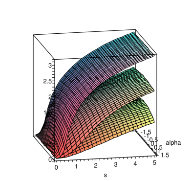
Figure 4. The Lyapunov exponent $\lambda_{p,s}(\alpha)$ as a function of $s$ and $\alpha$ for $p=1,\,2,\,5$.

Remark 6.2.

When $p=n\in\mathbb{N}$, we have

(6.7) $$\lambda_{n,s}(\alpha)=\sum_{k=0}^{n-1}\frac{n!}{2(n-k)k!}\left(\frac{\text{e}^{\text{i}\alpha}}{s}\right)^{k-n}\frac{K_{k}\left(\frac{2}{s}\text{e}^{\text{i}\alpha}\right)}{K_{n}\left(\frac{2}{s}\text{e}^{\text{i}\alpha}\right)}\,.$$

Indeed, the result follows from Theorem 4 and the formula (see §9.6.45 in [1])

$$\left[\frac{\partial}{\partial p}K_{p}(w)\right]_{p=n}=\sum_{k=0}^{n-1}\frac{n!}{2(n-k)k!}(w/2)^{k-n}K_{k}(w)\,.$$

The two most important special cases of (6.7) are:

1. The Lyapunov exponent for the generalized inverse Gaussian law.

   (6.8) $$\lambda_{n,s}(0)=\sum_{k=0}^{n-1}\frac{s^{n-k}n!}{2(n-k)k!}\frac{K_{k}(2/s)}{K_{n}(2/s)}.$$

2. The Lyapunov exponent for the Schrödinger case. Using the formula (see [24] §§3.6, 3.7)

   $$K_{n}(\text{i}w)=\frac{\pi}{2}\text{e}^{(3n+1)\frac{\pi\text{i}}{2}}(J_{n}(w)+\text{i}Y_{n}(w))$$

   one immediately obtains

   (6.9) $$\lambda_{n,s}(\pi/2)=\sum_{k=0}^{n-1}\frac{s^{n-k}n!}{2(n-k)k!}\frac{J_{k}(2/s)J_{n}(2/s)+Y_{k}(2/s)Y_{n}(2/s)}{J_{n}^{2}(2/s)+Y_{n}^{2}(2/s)}.$$

Next, we investigate the asymptotic behaviour of $\lambda_{p,s}(\alpha)$ for arbitrary positive $p$. In what follows, $\psi$ will denote the digamma function. We start with the large $s$ asymptotics.

Proposition 6.1.

For arbitrary $p>0$ and $\alpha\in[-\pi/2,\pi/2]$ we have the following large $s$ asymptotics of the Lyapunov exponent

(6.10) $$\lambda_{p,s}(\alpha)=\ln s+\psi(p)+R_{p,s}(\alpha),$$

where

(6.11) $$R_{p,s}(\alpha)=\begin{cases}2\cos(2p\alpha)\frac{\Gamma(1-p)}{\Gamma(1+p)}\frac{\ln s}{s^{2}}+O\left(1/s^{2}\right),&\text{if $p\in(0,1)$}\\ &\\ 2\cos(2\alpha)\frac{(\ln s)^{2}}{s^{2}}+O\left(\ln s/s^{2}\right),&\text{if $p=1$}\\ &\\ \frac{\cos(2\alpha)}{(p-1)^{2}}\frac{1}{s^{2}}+O\left(E(s)\right),&\text{if $p>1$}\\ \end{cases}$$

and

$$E(s)=\begin{cases}\ln s/s^{2p}&\text{if $p\in(1,2)$}\\ (\ln s)^{2}/s^{4}&\text{if $p=2$}\\ 1/s^{4}&\text{if $p>2$}\end{cases}\,.$$

Remark 6.3.

Although only the leading term of the expansion for the remainder $R_{p,s}$ is reported here, it will be clear from the proof that Formula (6.15) allows one to compute arbitrarily many terms.

Proof.

First, we note that, when $p\in{\mathbb{N}}$, the Lyapunov exponent is given explicitly by Equation (6.7), and its asymptotics can be deduced directly from the asymptotic expansion of the modified Bessel function of integral order (see §8.446 in [15]).

So, from now on, we shall assume that $p$ is not an integer. As a starting point, we take the following representations (Equations (8.485) and (8.445) in [15])

(6.12) $$K_{p}(w) = \frac{\pi}{2}\frac{I_{-p}(w)-I_{p}(w)}{\sin(p\pi)},$$

(6.13) $$I_{p}(w) = \left(\frac{w}{2}\right)^{p}\sum_{k=0}^{\infty}A_{k}(p)\left(\frac{w}{2}\right)^{2k},$$

where

$$A_{k,p}:=\frac{1}{k!\Gamma(p+k+1)}$$

These representations yield (cf. Equations (9.6.42-3) in [1])

$$\frac{\partial_{p}K_{p}(w)}{K_{p}(w)} = -\pi\cot(p\pi)+\frac{\partial_{p}I_{-p}(w)-\partial_{p}I_{p}(w)}{I_{-p}(z)-I_{p}(w)},$$

$$\partial_{p}I_{-p}(w) = -\ln\left(\frac{w}{2}\right)I_{-p}(w)+\left(\frac{w}{2}\right)^{-p}\sum_{k=0}^{\infty}B_{k}(-p)\left(\frac{w}{2}\right)^{2k},$$

$$\partial_{p}I_{p}(w) = \ln\left(\frac{w}{2}\right)I_{p}(w)-\left(\frac{w}{2}\right)^{p}\sum_{k=0}^{\infty}B_{k}(p)\left(\frac{w}{2}\right)^{2k},$$

where

$$B_{k,p}:=\frac{\psi(p+k+1)}{k!\Gamma(p+k+1)}\,.$$

Thus

(6.14) $$\Lambda_{p}(w)=-\pi\cot(p\pi)+\\ \frac{\sum_{k=0}^{\infty}\left(-A_{k,-p}\ln\left(\frac{w}{2}\right)+B_{k,-p}\right)\left(\frac{w}{2}\right)^{2k}-\left(A_{k,p}\ln\left(\frac{w}{2}\right)-B_{k,p}\right)\left(\frac{w}{2}\right)^{2(k+p)}}{\sum_{k=0}^{\infty}A_{k,-p}\left(\frac{w}{2}\right)^{2k}-A_{k,p}\left(\frac{w}{2}\right)^{2(k+p)}}\,.$$

For small $w$, we then have the asymptotic expansion

(6.15) $$\Lambda_{p}(w)\sim-\pi\cot(p\pi)+\Gamma(1-p)\times\\ \left[\sum_{k=0}^{\infty}\left(A_{k,-p}\ln\left(\frac{2}{w}\right)+B_{k,-p}\right)\left(\frac{w}{2}\right)^{2k}+\left(A_{k,p}\ln\left(\frac{2}{w}\right)+B_{k,p}\right)\left(\frac{w}{2}\right)^{2(k+p)}\right]\times\\ \left[1+\sum_{n=1}^{\infty}\left(\sum_{k=0}^{\infty}\Gamma(1-p)A_{k,p}\left(\frac{w}{2}\right)^{2(k+p)}-\sum_{k=1}^{\infty}\Gamma(1-p)A_{k,-p}\left(\frac{w}{2}\right)^{2k}\right)^{n}\right]\,.$$

Applying the identities (cf. Equation (8.365), Points (1) and (8), [15])

$$\psi(2-p)-\psi(1-p)=(1-p)^{-1},\qquad\psi(1-p)-\pi\cot(p\pi)=\psi(p),$$

and keeping only the most significant terms we obtain, for all positive noninteger $p$ and small $w$, the expansion

(6.16) $$\Lambda_{p}(w)\sim\ln(2/w)+\psi(p)+2\frac{\Gamma(1-p)}{\Gamma(1+p)}\ln(2/w)(w/2)^{2p}+\frac{1}{(1-p)^{2}}(w/2)^{2}+\cdots$$

The behavior of the error term depends on the value of $p$. For noninteger $p$ we have the following estimates of the error: $O(w^{2p})$ for $p\in(0,1)$; $O((\ln s)/w^{2p})$ for $p\in(1,2)$ and $O(w^{4})$ for $p>2$.

Substituting $w=2\text{e}^{\text{i}\alpha}/s$ and taking the real part (cf. Theorem 4) completes the proof. ∎

It is worth noting that, when $p$ is large, there is an alternative way of obtaining the asymptotics of the Lyapunov exponent. Indeed, by using the integral representation

$$K_{p}(z)=\frac{1}{2}\left(\frac{2}{z}\right)^{p}\int_{0}^{\infty}t^{p-1}e^{-t-\frac{z^{2}}{4t}}\,\text{d}t,$$

one easily deduces the following version of Equation (8.446) in [15]:

(6.17) $$K_{p}(z)\sim\frac{1}{2}\left(\frac{2}{z}\right)^{p}\sum_{0\leq k<p}\frac{\Gamma(p-k)}{k!}\left(-\frac{z^{2}}{4}\right)^{k},\quad\text{as $z\rightarrow 0$}\,.$$

This yields (6.10) for $p>2$ and explains the absence of “logarithmic” prefactors in the low order terms of the expansion for the Lyapunov exponent when $p$ is large.

Next, we turn to the case of small $s$.

Proposition 6.2.

For arbitrary $p>0$ and $\alpha\in[-\pi/2,\pi/2]$, we have the following small $s$ asymptotics of the Lyapunov exponent:

(6.18) $$\lambda_{p,s}(\alpha)\sim\sum_{n=1}^{\infty}l_{n}s^{n}\quad\text{as $s\rightarrow 0$},$$

where

(6.19) $$l_{1}=\frac{p\cos\alpha}{2},\quad l_{2}=-\frac{p\cos 2\alpha}{8},\quad l_{3}=-\frac{p(4p^{2}-13)\cos 3\alpha}{192},\\ l_{4}=\frac{p(4p^{2}-7)\cos 4\alpha}{128},\quad l_{5}=\frac{p(-920p^{2}+48p^{4}+1187)\cos 5\alpha}{20480}\,.$$

Remark 6.4.

Higher order terms can be derived using formula (6.21) below.

Remark 6.5.

When $\alpha=\pm\pi/2$ (and only in this case) the real part of all odd order terms in (6.18) vanish. Thus the leading order term in this particular case is quadratic (cf. Figures 4 and 5).

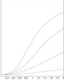
Figure 5. The Lyapunov exponent $\lambda_{p,s}(\pi/2)$ as a function of $s$. The curves in (a) are obtained by using the exact formula; those in (b) are obtained by summing the asymptotic series as $s\rightarrow 0$.

Proof.

For small $s$, the asymptotics follow from the behaviour of the modified Bessel functions for large $w$. We have (see [24] §7.23)

$$K_{p}(w)=\left(\frac{\pi}{2w}\right)^{1/2}\text{e}^{-w}\sum_{m=0}^{n-1}\frac{(p,m)}{(2w)^{m}}+\Theta(p)\frac{(p,n)}{(2w)^{n}},$$

where

$$(p,m):=\frac{\Gamma(p+m+1/2)}{m!\Gamma(p-m+1/2)}=\frac{(4p^{2}-1)(4p^{2}-3^{2})...(4p^{2}-(2m-1)^{2})}{2^{2m}m!}$$

and where the constant $\Theta$ satisfies

$$|\Theta|<1\quad\text{and}\quad\text{Re}\Theta\geq 0\qquad\text{for $p\in{\mathbb{R}}$ and $\text{Re}w\geq 0$}\,.$$

(If $n>p-1/2$, then $0\leq\Theta\leq 1$, see [24] §7.30). Thus, we have

(6.20) $$\frac{\partial_{p}K_{p}(w)}{K_{p}(w)}=\frac{\sum_{m=0}^{n-1}\frac{\partial_{p}(p,m)}{(2w)^{m}}+\frac{\partial_{p}(\Theta(p)(p,n))}{(2w)^{n}}}{\sum_{m=0}^{n-1}\frac{(p,m)}{(2w)^{m}}+\Theta(p)\frac{(p,n)}{(2w)^{n}}}\,,$$

where

$$\partial_{p}(p,m)=\frac{\Gamma(p+m+1/2)}{m!\Gamma(p-m+1/2)}[\psi(p+m+1/2)-\psi(p+m+1/2)].$$

This leads to the following expansion for large $w$

(6.21) $$\Lambda_{p}(w)\sim\left[\sum_{m=1}^{n-1}\frac{\partial_{p}(p,m)}{(2w)^{m}}+\frac{\partial_{p}(\Theta(p)(p,n))}{(2w)^{n}}\right]\times\\ \left[1+\sum_{N=1}^{\infty}\left(-\sum_{m=1}^{n-1}\frac{(p,m)}{(2w)^{m}}-\Theta(p)\frac{(p,n)}{(2w)^{n}}\right)^{N}\right]\,.$$

From this expansion, every coefficient in (6.18) can be computed explicitly. In particular, by using the basic properties of the gamma and digamma functions, we obtain

(6.22) $$\Lambda_{p}(w)\sim\frac{p}{w}-\frac{p}{2w^{2}}-\frac{p(4p^{2}-13)}{24w^{3}}+\\ \frac{p(4p^{2}-7)}{8w^{4}}+\frac{p(-920p^{2}+48p^{4}+1187)}{640w^{5}}-\cdots\quad\text{as $w\rightarrow\infty$}\,.$$

By setting $w=2\text{e}^{\text{i}\alpha}/s$ and taking the real part, one obtains Equation (6.19). ∎

Remark 6.6.

Although the series (6.18) is divergent, one can compute its sum by using standard summation techniques [4]. The plots of $\lambda_{p,s}(\pi/2)$ against $s$ for various half-integer values of $p$ shown in Figure 5 (b) were obtained by using a Padé approximant— i.e. a rational function of $s$ that matches the series to $O(s^{64})$.

Acknowledgments: We thank Brian Winn for a very helpful discussion leading to the discovery of Formula (6.1).

Appendix A Some identities involving products of Bessel functions

We begin with two integral representations of the modified Bessel function: For $\operatorname{Re}z>0$, we have (cf. [24], §6.22)

(A.1) $$K_{p}(z)=\frac{1}{2}\int_{0}^{\infty}t^{-p-1}\exp\left\{-\frac{z}{2}(t+1/t)\right\}\,\text{d}t\\ =\frac{z^{p}}{2}\int_{0}^{\infty}\tau^{-p-1}\exp\left\{-\frac{1}{2}\left(\tau+z^{2}/\tau\right)\right\}\,\text{d}\tau\,.$$

When calculating the moments of $\nu$, we will use integrals of the form

(A.2) $${\mathcal{I}}_{p}^{(n)}(u,v):=\frac{1}{2}\int_{0}^{\infty}\exp\left\{-\frac{\tau}{2}-\frac{u^{2}+v^{2}}{2\tau}\right\}K_{p}\left(\frac{uv}{\tau}\right)\tau^{n}\,\text{d}\tau,$$

where $n\in{\mathbb{Z}}$, and the complex numbers $u$ and $v$ are such that

$$|\arg u|<\pi,\quad|\arg v|<\pi\quad\text{and}\quad|\arg(u+v)|<\pi/4\,.$$

For $n=-1$, the value is given by Macdonald’s formula [24], §13.71:

(A.3) $${\mathcal{I}}_{p}^{(-1)}(u,v)=K_{p}(u)K_{p}(v)\,.$$

Differentiate this identity with respect to $u$, and then multiply it by $u$ to obtain

(A.4) $$uK_{p}^{\prime}(u)K_{p}(v)=\frac{1}{2}\int_{0}^{\infty}\exp\left\{-\frac{\tau}{2}-\frac{u^{2}+v^{2}}{2\tau}\right\}\left[-\frac{u^{2}}{\tau^{2}}K_{p}\left(\frac{uv}{\tau}\right)+\frac{uv}{\tau^{2}}K_{p}^{\prime}\left(\frac{uv}{\tau}\right)\right]\,\text{d}\tau\\ =\frac{1}{2}\int_{0}^{\infty}\exp\left\{-\frac{\tau}{2}-\frac{u^{2}+v^{2}}{2\tau}\right\}\left[-\frac{1}{2}+\frac{v^{2}-u^{2}}{2\tau^{2}}\right]K_{p}\left(\frac{uv}{\tau}\right)\text{d}\tau$$

after integration by parts. If we interchange $u$ and $v$, this becomes

(A.5) $$vK_{p}(u)K_{p}^{\prime}(v)\\ =\frac{1}{2}\int_{0}^{\infty}\exp\left\{-\frac{\tau}{2}-\frac{u^{2}+v^{2}}{2\tau}\right\}\left[-\frac{1}{2}-\frac{v^{2}-u^{2}}{2\tau^{2}}\right]K_{p}\left(\frac{uv}{\tau}\right)\text{d}\tau\,.$$

Hence, by adding these two identities, we find

(A.6) $${\mathcal{I}}_{p}^{(0)}(u,v)=uK_{p+1}(u)K_{p}(v)+vK_{p+1}(v)K_{p}(u)-2p\,K_{p}(u)K_{p}(v)\,.$$

By similar calculations, we obtain easily the recurrence relations

(A.7) $${\mathcal{I}}_{p}^{(n)}=\left[2n-u\frac{\partial}{\partial u}-v\frac{\partial}{\partial v}\right]\,{\mathcal{I}}_{p}^{(n-1)},\quad n\in{\mathbb{N}}\,.$$

and

(A.8) $$(v^{2}-u^{2}){\mathcal{I}}_{p}^{(n-1)}=\left[u\frac{\partial}{\partial u}-v\frac{\partial}{\partial v}\right]\,{\mathcal{I}}_{p}^{(n)},\quad n\in{\mathbb{Z}}\,.$$

The first of these enables the evaluation of the integral (A.2) in terms of products of modified Bessel functions when $n=0,1,\ldots$, whereas the second is appropriate when $n=-2,-3,\ldots$ (provided that $u^{2}\neq v^{2}$).

Appendix B Calculation of the moments

In this section, we show how to calculate the moments

(B.1) $$M_{p,s}^{(m,n)}(\alpha):=\int_{S_{\alpha}}z^{m}\bar{z}^{n}\,f(z)\,\text{d}z,\quad m,n\in{\mathbb{N}},$$

of the distribution $\nu$. For simplicity, we shall assume that $\alpha>0$.

We have

(B.2) $$M_{p,s}^{(m,n)}(\alpha)=\int_{-\alpha}^{\alpha}\int_{0}^{\infty}r^{m+n}\text{e}^{\text{i}(m-n)\theta}\,\frac{c_{p,s}(\alpha)\sin(2\alpha)}{r^{2}\sin^{2}(\alpha+\theta)}\left[\frac{\sin(\alpha-\theta)}{\sin(\alpha+\theta)}\right]^{p-1}\\ \times\exp\left\{-\frac{\sin(2\alpha)}{s}\left[\frac{1}{r\sin(\alpha-\theta)}+\frac{r}{\sin(\alpha+\theta)}\right]\right\}\,r\text{d}r\text{d}\theta\,.$$

The substitution

$$t=\frac{\sin(\alpha-\theta)}{\sin(\alpha+\theta)}$$

yields

$$\text{d}t=-\frac{\sin(2\alpha)}{\sin^{2}(\alpha+\theta)}\,\text{d}\theta,\;\;\text{e}^{\text{i}\theta}=\frac{\text{e}^{\text{i}\alpha}+t\text{e}^{-\text{i}\alpha}}{\sqrt{t\varphi(t)}}$$

and

$$\frac{2\sin(2\alpha)}{s\sqrt{\sin(\alpha-\theta)\sin(\alpha+\theta)}}=\frac{2}{s}\sqrt{\varphi(t)},$$

where

$$\varphi(t)=t+1/t+2\cos(2\alpha)\,.$$

Hence

(B.3) $$M_{p,s}^{(m,n)}(\alpha)=c_{p,s}(\alpha)\int_{0}^{\infty}\int_{0}^{\infty}r^{m+n-1}t^{p-1}\left[\frac{\text{e}^{\text{i}\alpha}+t\text{e}^{-\text{i}\alpha}}{\sqrt{t\varphi(t)}}\right]^{m-n}\\ \times\exp\left\{-\frac{1}{s}\left[\frac{1}{r}\sqrt{\frac{\varphi(t)}{t}}+r\sqrt{t\varphi(t)}\right]\right\}\text{d}r\text{d}t$$

Next, we make the change of variable

$$r=\frac{2}{s\tau}\sqrt{\frac{\varphi(t)}{t}}$$

to obtain

(B.4) $$M_{p,s}^{(m,n)}(\alpha)=c_{p,s}(\alpha)\left(\frac{2}{s}\right)^{m+n}\int_{0}^{\infty}\int_{0}^{\infty}\frac{t^{p-m-1}}{\tau^{m+n+1}}\varphi^{n}(t)\left(\text{e}^{\text{i}\alpha}+t\text{e}^{-\text{i}\alpha}\right)^{m-n}\\ \times\exp\left\{-\frac{\tau}{2}-\frac{2\varphi(t)}{s^{2}\tau}\right\}\text{d}\tau\text{d}t\\ =c_{p,s}(\alpha)\left(\frac{2}{s}\right)^{m+n}\int_{0}^{\infty}\int_{0}^{\infty}\frac{t^{p-m-1}}{\tau^{m+n+1}}\left[t+1/t+2\cos(2\alpha)\right]^{n}\left(\text{e}^{\text{i}\alpha}+t\text{e}^{-\text{i}\alpha}\right)^{m-n}\\ \times\exp\left\{-\frac{2}{s^{2}\tau}\left(t+\frac{1}{t}\right)\right\}\exp\left\{-\frac{\tau}{2}-\frac{4\cos(2\alpha)}{s^{2}\tau}\right\}\text{d}t\text{d}\tau\,.$$

By using the fact that

$$K_{q}(z)=\frac{1}{2}\,\int_{0}^{\infty}t^{q-1}\exp\left\{-\frac{z}{2}(t+1/t)\right\}\,\text{d}t,$$

we can, provided that $n\leq m$, express this double integral in terms of the integrals (A.2). For instance, when $m=n=0$, Equation (B.4) yields

(B.5) $$1=M_{p,s}^{(0,0)}(\alpha)\\ =c_{p,s}(\alpha)\int_{0}^{\infty}\exp\left\{-\frac{\tau}{2}-\frac{4\cos(2\alpha)}{s^{2}\tau}\right\}\int_{0}^{\infty}t^{p-1}\exp\left\{-\frac{2}{s^{2}\tau}\left(t+\frac{1}{t}\right)\right\}\text{d}t\frac{\text{d}\tau}{\tau}\\ =2\,c_{p,s}(\alpha)\int_{0}^{\infty}\exp\left\{-\frac{\tau}{2}-\frac{4\cos(2\alpha)}{s^{2}\tau}\right\}K_{p}\left(\frac{4}{s^{2}\tau}\right)\frac{\text{d}\tau}{\tau}\,.$$

This can be expressed as

$$1=M_{p,s}^{(0)}(\alpha)=4\,c_{p,s}(\alpha)\,{\mathcal{I}}_{p}^{(-1)}\left(u,v\right),\quad u=\overline{v}=2\text{e}^{\text{i}\alpha}/s\,.$$

So we deduce the value of the normalisation constant from Equation (A.3). In the same way, by taking $m=1$ and $n=0$, we obtain the mean:

$${\mathbb{E}}\left(Z\right)=M_{p,s}^{(1,0)}(\alpha)=4\,c_{p,s}(\alpha)\left\{v{\mathcal{I}}_{p-1}^{(-2)}\left(u,v\right)+u{\mathcal{I}}_{p}^{(-2)}\left(u,v\right)\right\}\,.$$

Its value is given by Equation (3.18). For the variance, we use

$$\text{Var}\left(Z\right)=M_{p,s}^{(1,1)}(\alpha)-\left|M_{p,s}^{(1,0)}(\alpha)\right|^{2}\,.$$

Equation (B.4) gives

$$M_{p,s}^{(1,1)}(\alpha)=4\,c_{p,s}(\alpha)\left(\frac{2}{s}\right)^{2}\left\{{\mathcal{I}}_{p-2}^{(-3)}(u,v)+2\cos(2\alpha)\,{\mathcal{I}}_{p-1}^{(-3)}(u,v)+{\mathcal{I}}_{p}^{(-3)}(u,v)\right\}$$

and so we deduce the value given in Equation (3.19).

Appendix C The Formula for the Lyapunov exponent

In this appendix, we consider matrices distributed according to a measure $\mu$ on $SL(2,\mathbb{C})$ of the form

$${\mathcal{A}}=\begin{bmatrix}a&b\\ c&d\\ \end{bmatrix}$$

with exactly one row being random. In other words, the measure $\mu$ is such that one or the other of the following conditions holds:

(I) $$a b c d$$ and are fixed, and are random

or

(II) $$\text{$c$ and $d$ are fixed, $a$ and $b$ are random}\,.$$

Let $\nu$ be $\mu$-invariant measure on the projective space $\mathbb{P}(\mathbb{C}^{2})=\bar{\mathbb{C}}$. In this case, we have (cf. Equation (1) in [6], p. 9)

$$\int_{\mathbb{C}}\int_{SL(2,\mathbb{C})}\varphi({\mathcal{A}}\cdot z)d\mu(\mathcal{A})d\nu(z)=\int_{\mathbb{P}(\mathbb{C}^{2})}\varphi(z)d\nu(z)$$

for every bounded Borel function $\varphi$.

First, let us consider the case where Condition (I) holds. Assume that $\nu$ has some positive moment. Suppose also that $\mu$ satisfies the conditions required for the existence and positivity of the Lyapunov exponent $\lambda$ (see Theorem 3.6 in [6], p. 27— which holds also in the complex domain). Then

(C.1) $$\lambda=\int_{\mathbb{C}}\int_{SL(2,\mathbb{C})}\ln\frac{\left|{\mathcal{A}}\binom{z}{1}\right|}{\left|\binom{z}{1}\right|}\,\text{d}\mu(\mathcal{A})\,\text{d}\nu(z)=\\ \frac{1}{2}\int_{\mathbb{C}}\int_{SL(2,\mathbb{C})}\ln\frac{|az+b|^{2}+|cz+d|^{2}}{|z|^{2}+1}\,\text{d}\mu(\mathcal{A})\,\text{d}\nu(z)=\\ \frac{1}{2}\int_{\mathbb{C}}\int_{SL(2,\mathbb{C})}\ln\left(1+|\mathcal{A}\cdot z|^{-2}\right)+\ln\frac{|az+b|^{2}}{|z|^{2}+1}\,\text{d}\mu(\mathcal{A})\,\text{d}\nu(z)=\\ \frac{1}{2}\int_{\mathbb{C}}\ln\left(1+|z|^{-2}\right)\,\text{d}\nu(z)+\int_{\mathbb{P}(\mathbb{C}^{2})}\ln\left|a+bz^{-1}\right|\,\text{d}\nu(z)\\ -\frac{1}{2}\int_{\mathbb{C}}\ln\left(1+|z|^{-2}\right)\,\text{d}\nu(z)=\int_{\mathbb{C}}\ln\left|a+bz^{-1}\right|\,\text{d}\nu(z).$$

We note that the splitting of the integrals in this calculation is permissible because the assumed existence of a positive moment of $\mu$ guarantees the integrability of $\ln(1+|z|^{-2})$ and $\ln(a+b|z|^{-1})$.

The case where Condition (II) holds involves a similar calculation; hence

(C.2) $${\lambda}=\begin{cases}\int_{\mathbb{C}}\ln|a+bz^{-1}|\,\text{d}{\nu}(z)&\text{if Condition (\ref{caseI}) holds}\\ &\\ \int_{\mathbb{C}}\ln|cz+d|\,\text{d}{\nu}(z)&\text{if Condition (\ref{caseII}) holds}\end{cases}\,.$$

Now, we apply this result to the matrices (2.3) considered in Section 2. In this case, Condition (I) holds; there is only one random entry, and since it is gamma-distributed, the support of $\mu$ is not contained in any compact subgroup of $\text{GL}(2,{\mathbb{C}})$. Furthermore

$${\mathcal{A}}^{*}_{n}(\alpha)={\mathcal{A}}_{n}(-\alpha)$$

and hence the invariant measure for ${\mathcal{A}}^{*}_{n}(\alpha)$ is continuous for all $\alpha\in[-\pi/2,\pi/2]$. We may therefore use Proposition 3.3 in [6], p. 26, to deduce the uniqueness of the invariant measure $\nu$ found in the paper. Since, for all $\alpha\in[-\pi/2,\pi/2]$, this measure possesses positive moments of all orders less then one, we can apply Formula (C.2) to obtain (2.12).

For matrices of the form (2.14) and for Schrödinger matrices, it is Condition (II) that holds, and the formula (C.2) leads to (2.15).

Appendix D Proof of Theorem 1

Proof.

By direct substitution in Equation (3.4). To facilitate the calculation, define

(D.1) $$r_{a}=\sqrt{(x-a\cos\alpha)^{2}+(y-a\sin\alpha)^{2}},\\ X_{a}=-\frac{(x-a\cos\alpha)\sin\alpha+(y-a\sin\alpha)\cos\alpha}{r_{a}^{2}}\quad\text{and}\\ Y_{a}=(y-a\sin\alpha)\cos\alpha-(x-a\cos\alpha)\sin\alpha\,.$$

We note that

$$r_{0}=r,\quad X_{0}=X\quad\text{and}\quad Y_{a}\equiv Y\,.$$

We can write

(D.2) $$f_{\alpha}(z-a\text{e}^{\text{i}\alpha})\gamma_{p,s}(a)=CY^{p-1}\exp\left\{\frac{\sin(2\alpha)}{s}\frac{1}{Y}\right\}\\ \times\frac{a^{p-1}}{s^{p}\Gamma(p)}\left[r_{a}^{2}X_{a}\right]^{-(p+1)}\exp\left\{E(a)/s\right\},$$

where

$$E(a)=\frac{\sin(2\alpha)}{X_{a}}-a\,.$$

A lengthy but straightforward calculation reveals that

$$E^{\prime}(a)=-\left[\frac{Y}{r_{a}^{2}X_{a}}\right]^{2}\,.$$

Hence, by integrating Equation (D.2) with respect to $a$, we obtain

(D.3) $$\int_{0}^{a(x,y)}f_{\alpha}(z-a\text{e}^{\text{i}\alpha})\gamma_{p,s}(a)\,\text{d}a=C\frac{Y^{p-1}}{Y^{2}}\exp\left\{\frac{\sin(2\alpha)}{s}\frac{1}{Y}\right\}\,{\mathcal{E}}_{p},$$

where

$${\mathcal{E}}_{p}=-\int_{0}^{a(x,y)}\frac{1}{s^{p}\Gamma(p)}\left[\frac{a}{r_{a}^{2}X_{a}}\right]^{p-1}E^{\prime}(a)\exp\left\{E(a)/s\right\}\,\text{d}a\,.$$

Noting that

$$\frac{\text{d}}{\text{d}a}\left[\frac{a}{r_{a}^{2}X_{a}}\right]=-\frac{x\sin\alpha+y\cos\alpha}{r_{a}^{4}X_{a}^{2}}=\frac{r^{2}X}{r_{a}^{4}X_{a}^{2}}=-\frac{r^{2}X}{Y^{2}}E^{\prime}(a),$$

we obtain, after integration by parts,

(D.4) $${\mathcal{E}}_{p}=\left.\frac{-1}{s^{p-1}\Gamma(p)}\left[\frac{a}{r_{a}^{2}X_{a}}\right]^{p-1}\exp\left\{E(a)/s\right\}\right|_{0}^{a(x,y)}+\begin{cases}0&\text{if $p=1$}\\ \frac{r^{2}X}{Y^{2}}{\mathcal{E}}_{p-1}&\text{if $p>1$}\end{cases}\\ =\begin{cases}\exp\left\{E(0)/s\right\}&\text{if $p=1$}\\ \frac{r^{2}X}{Y^{2}}{\mathcal{E}}_{p-1}&\text{if $p>1$}\end{cases}\,.$$

Thus,

$${\mathcal{E}}_{p}=\left[\frac{r^{2}X}{Y^{2}}\right]^{p-1}\,\exp\left\{\frac{\sin(2\alpha)}{s}\frac{1}{X}\right\}$$

and, reporting this in Equation (D.3), we have shown that

(D.5) $$\int_{0}^{a(x,y)}f_{\alpha}(z-a\text{e}^{\text{i}\alpha})\gamma_{p,s}(a)\,\text{d}a\\ =\frac{C}{Y^{2}}\left(\frac{r^{2}X}{Y}\right)^{p-1}\exp\left\{\frac{\sin(2\alpha)}{s}\left[\frac{1}{Y}+\frac{1}{X}\right]\right\}\,.$$

It follows easily that $f_{\alpha}$ satisfies Equation (3.4). ∎

Appendix E Proof of Theorem 2

Proof.

We need only consider the case $\alpha=\pi/2$. As in the case $|\alpha|<\pi/2$, the proof is by direct substitution of the expression

$$f_{+}(y)=\frac{1}{y^{p+1}}\exp\left[\frac{1}{s}\left(\frac{1}{y}-y\right)\right]\int_{c(y)}^{y}\exp\left[-\frac{1}{s}\left(\frac{1}{t}-t\right)\right]\,t^{p-1}\,\text{d}t\,,$$

where

$$c(y)=\begin{cases}-\infty&\text{if $y<0$}\\ 0&\text{if $y>0$}\end{cases},$$

into the integral equation (4.3).

By making the substitution $u=-1/y-a$ in the integral on the right-hand side of Equation (4.3), we obtain

(E.1) $$\frac{1}{y^{2}}\int_{0}^{\infty}f_{+}\left(-\frac{1}{y}-a\right)\gamma_{p,s}(a)\text{d}a\\ =\frac{1}{y^{2}}\int_{-\infty}^{-1/y}f_{+}(u)\gamma_{p,s}\left(-\frac{1}{y}-u\right)\text{d}u\\ =\frac{1}{y^{2}}\int_{-\infty}^{-1/y}\int_{c(u)}^{u}\frac{1}{u^{p+1}}\exp\left[\frac{1}{s}\left(\frac{1}{u}-\frac{1}{t}+t+\frac{1}{y}\right)\right]\\ \times t^{p-1}\frac{1}{s^{p}\Gamma(p)}\left(-\frac{1}{y}-u\right)^{p-1}\text{d}t\text{d}u\,.$$

At this point, it is helpful to treat the cases $y<0$ and $y>0$ separately.

Let us begin by assuming that $y>0$. Then $c(u)=-\infty$ on the right-hand side of the last equation and, by changing the order of integration, we obtain

(E.2) $$\frac{1}{y^{2}}\int_{0}^{\infty}f_{+}\left(-\frac{1}{y}-a\right)\gamma_{p,s}(a)\text{d}a\\ =\frac{\text{e}^{\frac{1}{sy}}}{y^{p+1}}\int_{-\infty}^{-1/y}\exp\left[-\frac{1}{s}\left(\frac{1}{t}-t\right)\right]\\ \times t^{p-1}\int_{t}^{-1/y}\frac{1}{s^{p}\Gamma(p)}\left(-\frac{1}{u}-y\right)^{p-1}\text{e}^{\frac{1}{su}}\frac{1}{u^{2}}\text{d}u\text{d}t\,.$$

Then, after making the substitution $\tau=-1/t$, followed by $v=1/u+y$, this becomes

(E.3) $$\frac{1}{y^{2}}\int_{0}^{\infty}f_{+}\left(-\frac{1}{y}-a\right)\gamma_{p,s}(a)\text{d}a\\ =\frac{1}{y^{p+1}}\exp\left[\frac{1}{s}\left(\frac{1}{y}-y\right)\right]\int_{0}^{y}\exp\left[-\frac{1}{s}\left(\frac{1}{\tau}-\tau\right)\right]\frac{1}{\tau^{p+1}}\varphi(y-\tau)\text{d}\tau,$$

where

(E.4) $$\varphi(w)=\int_{0}^{w}\frac{1}{s^{p}\Gamma(p)}v^{p-1}\text{e}^{\frac{v}{s}}\text{d}v\,.$$

In order to prove that Equation (4.3) holds for $y>0$, we therefore only need to verify that

$$\int_{0}^{y}\exp\left[-\frac{1}{s}\left(\frac{1}{t}-t\right)\right]t^{p-1}\text{d}t=\int_{0}^{y}\exp\left[-\frac{1}{s}\left(\frac{1}{t}-t\right)\right]\frac{1}{t^{p+1}}\varphi(y-t)\text{d}t$$

holds identically for every $y>0$. Clearly, it holds when $y=0+$, and so it will be sufficient to show that the derivatives are the same. The derivative of the right-hand side is

(E.5) $$\exp\left[-\frac{1}{s}\left(\frac{1}{y}-y\right)\right]\frac{1}{y^{p+1}}\varphi(0)+\int_{0}^{y}\exp\left[-\frac{1}{s}\left(\frac{1}{t}-t\right)\right]\frac{1}{t^{p+1}}\varphi^{\prime}(y-t)\text{d}t\\ =\int_{0}^{y}\exp\left[-\frac{1}{s}\left(\frac{1}{t}-t\right)\right]\frac{1}{t^{p+1}}\frac{1}{s^{p}\Gamma(p)}(y-t)^{p-1}\exp\left[\frac{1}{s}(y-t)\right]\text{d}t\\ =y^{p-1}\text{e}^{\frac{y}{s}}\int_{0}^{y}\frac{1}{s^{p}\Gamma(p)}\left(\frac{1}{t}-\frac{1}{y}\right)^{p-1}\text{e}^{-\frac{1}{st}}\frac{1}{t^{2}}\text{d}t\\ =y^{p-1}\exp\left[-\frac{1}{s}\left(\frac{1}{y}-y\right)\right]\int_{0}^{\infty}\frac{1}{s^{p}\Gamma(p)}u^{p-1}\text{e}^{-\frac{u}{s}}\text{d}u,$$

after making the substitution $u=1/t-1/y$. The result follows.

To complete the proof, we also need to consider the case $y<0$. Returning to Equation (E.1), we need to split the range of integration of the variable $u$ into positive and negative values. Recalling the definition of $c(u)$ and, as before, changing the order of integration, we obtain

(E.6) $$\frac{1}{y^{2}}\int_{0}^{\infty}f_{+}\left(-\frac{1}{y}-a\right)\gamma_{p,s}(a)\text{d}a\\ =\frac{\text{e}^{\frac{1}{sy}}}{y^{p+1}}\int_{-\infty}^{0}\exp\left[-\frac{1}{s}\left(\frac{1}{t}-t\right)\right]\\ \times t^{p-1}\int_{t}^{0}\frac{1}{s^{p}\Gamma(p)}\left(-\frac{1}{u}-y\right)^{p-1}\text{e}^{\frac{1}{su}}\frac{1}{u^{2}}\text{d}u\text{d}t\\ =\frac{\text{e}^{\frac{1}{sy}}}{y^{p+1}}\int_{0}^{-1/y}\exp\left[-\frac{1}{s}\left(\frac{1}{t}-t\right)\right]\\ \times t^{p-1}\int_{t}^{-1/y}\frac{1}{s^{p}\Gamma(p)}\left(-\frac{1}{u}-y\right)^{p-1}\text{e}^{\frac{1}{su}}\frac{1}{u^{2}}\text{d}u\text{d}t\,.$$

After making the substitution $v=-1/u-y$, this becomes

(E.7) $$\frac{1}{y^{2}}\int_{0}^{\infty}f_{+}\left(-\frac{1}{y}-a\right)\gamma_{p,s}(a)\text{d}a\\ =\frac{1}{y^{p+1}}\exp\left[\frac{1}{s}\left(\frac{1}{y}-y\right)\right]\int_{-\infty}^{-1/y}\exp\left[-\frac{1}{s}\left(\frac{1}{t}-t\right)\right]\phi(-1/t-y)t^{p-1}\text{d}t\\ -\frac{1}{y^{p+1}}\exp\left[\frac{1}{s}\left(\frac{1}{y}-y\right)\right]\int_{0}^{-1/y}\exp\left[-\frac{1}{s}\left(\frac{1}{t}-t\right)\right]t^{p-1}\text{d}t,$$

where

$$\phi(w)=\int_{w}^{\infty}\frac{1}{s^{p}\Gamma(p)}v^{p-1}\text{e}^{-\frac{v}{s}}\text{d}v\,.$$

Therefore, we have to prove that

(E.8) $$\int_{-\infty}^{y}\exp\left[-\frac{1}{s}\left(\frac{1}{t}-t\right)\right]t^{p-1}\text{d}t\\ =\int_{-\infty}^{-1/y}\exp\left[-\frac{1}{s}\left(\frac{1}{t}-t\right)\right]\phi(-1/t-y)t^{p-1}\text{d}t\\ -\int_{0}^{-1/y}\exp\left[-\frac{1}{s}\left(\frac{1}{t}-t\right)\right]t^{p-1}\text{d}t$$

holds for every $y<0$ . On both sides, the limit as $y\rightarrow-\infty$ is zero. Furthermore, the derivative of the right-hand side is

(E.9) $$\exp\left[-\frac{1}{s}\left(\frac{1}{y}-y\right)\right]\frac{(-1)^{p-1}}{y^{p+1}}\left[\phi(0)-1\right]\\ -\int_{-\infty}^{-1/y}\exp\left[-\frac{1}{s}\left(\frac{1}{t}-t\right)\right]t^{p-1}\phi^{\prime}(-1/t-y)\\ =\int_{-\infty}^{-1/y}\exp\left[-\frac{1}{s}\left(\frac{1}{t}-t\right)\right]t^{p-1}\frac{1}{s^{p}\Gamma(p)}\left(-\frac{1}{t}-y\right)^{p-1}\exp\left[-\frac{1}{s}\left(-\frac{1}{t}-y\right)\right]\text{d}t\\ =y^{p-1}\text{e}^{\frac{y}{s}}\int_{-\infty}^{-1/y}\frac{1}{s^{p}\Gamma(p)}\left(-\frac{1}{y}-t\right)^{p-1}\text{e}^{\frac{t}{s}}\text{d}t\\ =y^{p-1}\exp\left[-\frac{1}{s}\left(\frac{1}{y}-y\right)\right]\int_{0}^{\infty}\frac{1}{s^{p}\Gamma(p)}v^{p-1}\text{e}^{-v}\text{d}v$$

after making the substitution $v=-1/y-t$. ∎

Appendix F An asymptotic expansion for $f_{+}$ as $s\rightarrow 0$

It is actually simpler to work with

$$u(y)=\frac{1}{y^{2}}f_{+}(-1/y)\,.$$

So let write

$$u(y)\sim\sum_{n=1}^{\infty}u^{(n)}(y)s^{n}\quad\text{as $s\rightarrow 0$}\,.$$

where

$$u^{(n)}(y)=\frac{1}{y^{2}}f_{+}^{(n)}(-1/y)\,.$$

Equation (4.13) then gives

(F.1) $$u^{(1)}(y)=\frac{1}{1+y^{2}}\quad\text{and}\quad u^{(n+1)}(y)=\frac{-y^{p+1}}{1+y^{2}}\frac{\text{d}}{\text{d}y}\left[\frac{u^{(n)}(y)}{y^{p-1}}\right]\,.$$

A direct calculation of the first few terms reveals that the $u^{(n)}$ have a very simple structure:

(F.2) $$u^{(2n-1)}(y)=\sum_{k=n}^{4n-3}\frac{u_{k}^{(2n-1)}}{(1+y^{2})^{k}}\quad\text{and}\quad u^{(2n)}(y)=\sum_{k=n+1}^{4n-1}\frac{u_{k}^{(2n)}y}{(1+y^{2})^{k}},\quad u_{k}^{(n)}\in{\mathbb{R}}\,.$$

By substituting these expressions in Equation (F.1), one obtains the recurrence relations

$$u_{n+1}^{(2n)} =(p-1+2n)u_{n}^{(2n-1)},$$

$$u_{k}^{(2n)} =(p-3+2k)u_{k-1}^{(2n-1)}-2(k-2)u_{k-2}^{(2n-1)},\quad n+2\leq k\leq 4n-2,$$

$$u_{4n-1}^{(2n)} =-2(4n-3)u_{4n-3}^{(2n-1)},$$

$$u_{n+1}^{(2n+1)} =(p+2n)u_{n+1}^{(2n)},$$

$$u_{n+2}^{(2n+1)} =(p+2n+2)u_{n+2}^{(2n)}-(p+2+4n)u_{n+1}^{(2n)},$$

$$u_{k}^{(2n+1)} =(p-2+2k)u_{k}^{(2n)}$$

$$+(6-p-4k)u_{k-1}^{(2n)}+2(k-2)u_{k-2}^{(2n)},\quad n+3\leq k\leq 4n-1,$$

$$u_{4n}^{(2n+1)} =(6-p-16n)u_{4n-1}^{(2n)}+2(4n-2)u_{4n-2}^{(2n)},$$

$$u_{4n+1}^{(2n+1)} =(8n-2)u_{4n-1}^{(2n)},$$

with the starting value $u_{1}^{(1)}=1$. We then have

(F.3) $$\int_{{\mathbb{R}}}f_{+}(y)\text{d}y=\int_{{\mathbb{R}}}u(y)\text{d}y\sim 2\sum_{n=1}^{\infty}s^{2n-1}\sum_{k=n}^{4n-3}u_{k}^{(2n-1)}\alpha_{k}$$

and

(F.4) $$-\int_{\mathbb{R}}\ln|y|\,f_{\pi/2}(y)\text{d}y=\int_{\mathbb{R}}\ln|y|\,u(y)\text{d}y\sim 2\sum_{n=1}^{\infty}s^{2n-1}\sum_{k=n}^{4n-3}u_{k}^{(2n-1)}\beta_{k}$$

as $s\rightarrow 0$, where

$$\alpha_{k}=\int_{0}^{\infty}\frac{\text{d}y}{(1+y^{2})^{k}}\quad\text{and}\quad\beta_{k}=\int_{0}^{\infty}\frac{\ln y\,\text{d}y}{(1+y^{2})^{k}}\,.$$

The $\alpha_{k}$ and $\beta_{k}$ satisfy the recurrence relations

$$\alpha_{k+1}=\left(1-\frac{1}{2k}\right)\alpha_{k},\quad\beta_{k+1}=\beta_{k}-\frac{\alpha_{k}+\beta_{k}}{2k},\quad\alpha_{1}=\frac{\pi}{2},\;\beta_{1}=0\,.$$

References

[1] M. Abramowitz and I.A. Stegun, Handbook of Mathematical Functions. Dover, 1964
[2] P. W. Anderson, Absence of diffusion in certain random lattices.
Phys. Rev. 109, 1492-1505 (1958).
[3] G. A. Baker and P. Graves–Morris, Padé
Approximants, Cambridge University Press, Cambridge, 1996.
[4] C. Bender & S. A. Orszag, Advanced
Mathematical Methods for Scientists and Engineers,
McGraw–Hill, New York, 1978.
[5] E. Bernadac, Random continued fractions and inverse gaussian distribution
on a symmetric cone, J. Th. Prob.8 (1995) 221-259.
[6] P. Bougerol and J. Lacroix, Products of
Random Matrices with Applications to Schrödinger Operators,
Birkhäuser, 1985.
[7] R. Carmona and J. Lacroix, Spectral Theory of
Random Schrödinger Operators, Birkhäuser, 1990.
[8]
R. Carmona, A. Klein and F. Martinelli, Anderson localization for Bernoulli and other singular potentials.
Comm. Math. Phys.108 (1987), no. 1, 41–66.
[9] J. F. Chamayou and G. Letac, Explicit stationary distributions
for compositions of random functions and products of random matrices,
J. Th. Prob.4 (1991) 3-36.
[10] A. Comtet,
Private communication.
[11] P. Diaconis and D. Freedman, Iterated random functions,
SIAM Rev41 (1999) 41-66.
[12] F. J. Dyson, The dynamics of a disordered linear chain, Phys. Rev.92
(1953) 1331-1338.
[13] H. Furstenberg, Non commuting random products, Trans. Amer. Math. Soc.108 (1963) 377-428.
[14] H. Furstenberg and H. Kesten, Products of random matrices.
Ann. Math. Statist.31 (1960) 377-428.
[15] I.S. Gradshteyn and I.M. Ryzhik, Table of integrals series and products
Academic Press, New York, 1965.
[16] D.C. Herbert and R. Jones, Localized states in disordered systems
J. Phys. C. Solid State Phys.4, (1971) 1145-61.
[17]
H. Knuz, B. Souillard, Sur le spectre des opérateurs aux différences finies aléatoires
Comm. Math. Phys.78 (1980), no. 2, 201–246.
[18] G. Letac and V. Seshadri, A characterisation of the
generalised inverse gaussian distribution by continued fractions,
Z. Wahrsch. Verw. Gebiete62
(1983) 485-489.
[19] G. Letac and V. Seshadri, A random continued fraction in
with an inverse Gaussian distribution,
Bernoulli1
(1995) 381-393.
[20] P. Lloyd, Exactly solvable model of electronic states in a three-dimensional disordered Hamiltonian:
non-existence of localized states J. Phys. C. Solid State Phys.2 (1969) 1717-25.
[21] A. N. Shiryaev, Probability (2nd ed.), Springer,
New-York, 1996.
[22] D.J. Thouless, A relation between the density of states and range of localization
for one dimensional random systems J. Phys. C. Solid State Phys.5 (1972) 78-81.
[23] Y. Tourigny and P. G. Drazin, The dynamics
of Padé approximation.
Nonlinearity15, 787-805 (2002).
[24] G. N. Watson, Theory of Bessel Functions, Cambridge University
Press, Cambridge, 1922.