Bound states of scalar particles in the presence of a short range potential

Abstract

We analyze the behavior of the energy spectrum of the Klein-Gordon equation in the presence of a truncated hyperbolic tangent potential. From our analysis we obtain that, for some values of the potential there is embedding of the bound states into the negative energy continuum, showing that, in opposition to the general belief, relativistic scalar particles in one-dimensional short range potentials can exhibit resonant behavior and not only the Schiff-Snyder effect.

The study of relativistic scalar particles in the presence of strong electromagnetic and gravitational fields is a topic that has been carefully discussed in the literatureGreiner1 ; Greiner , mainly because their implications in quantum phenomena like superradiance and black hole evaporationFulling as well as their astrophysical implications in the study of boson stars. Recently research has been conducted on quantum effects of Klein-Gordon particles in the presence of strong magnetic fieldsKhalilov ; Khalilov2 . The pioneering works on Klein-Gordon particles (pion, etc) date back to 1940 when Schiff, Snyder and Weinberg solved the Klein-Gordon equation for a square-well potential. A surprising outcome of this paper was that for strong potentials antiparticles states emerge from the lower continuum. A systematic study of the solutions of the Klein-Gordon equation for various types of potentials, aiming to investigate the conditions necessary for antiparticle binding, were performed by Fleischer and SoffFleischer .

Quantum effects associated with scalar particles in strong short-range electric fields exhibit some particularities that establish a fundamental difference between the eigenvalues and phase shifts for Dirac particles and Klein-Gordon particles when the intensity of the external potential surpasses the supercritical value. The bound $s$ state associated with the Klein-Gordon equation does not disappear and it does not behave like a resonance in the lower continuum of the energy spectrum. Such a state becomes a complex eigenstate with zero norm. Bawin and LavineBL:79 have shown that, for $p$ waves the eigenvalue becomes complex without the appearance of the Schiff - Snyder - Weinberg effect, phenomenon that takes place for $s$ waves and consists in the coalescence of particle and antiparticle eigenstates before they become complexSSW:40 ; Weinberg . It is worth mentioning that, since the Schiff-Snyder effect is a particular effect associated with short-range interacting potentials, it is not observed in the presence of Coulomb interactionsRafelski

In this article, using the phase shift approach Newton and the Wigner time delay EW:55 , we show that the phenomenon described in Ref. BL:79 also takes place for $s$ waves in the presence of a radial hyperbolic tangent potential. The potential is different from zero in the range $[0,a]$, with $a>0$ transforming the potential into a short-range potential. For this potential, with a judicious choice of the parameters (Fig. 1), we observe the phenomenon of resonance, which manifests itself via the the embedding in the lower negative continuum. This situation becomes a counterexample to the general result shown by Popov VP:71 according to which, for short-range potentials, $s$ waves solutions always exhibit the Schiff-Snyder-Weinberg effect and therefore there is no embedding of the bound states into the negative continuum.

The radial equation for $s$ waves is given by Greiner

$$\frac{d^{2}u(r)}{dr^{2}}+\left(\left(E-V(r)\right)^{2}-m^{2}\right)u(r)=0$$ (1)

where $eA_{0}=V(r)$ with

$$V(r)=\begin{cases}D\tanh(kr)-B,&\,r\in[0,a],\\ 0,&\,r\in[a,\infty).\end{cases}$$ (2)

and we have adopted the natural units $\hslash=c=1$,

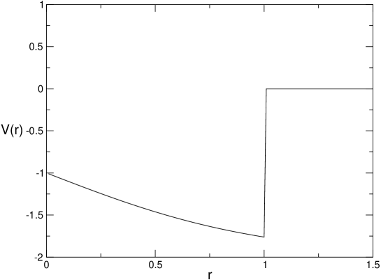
Figure 1: Plot of the truncated hyperbolic tangent potential for $D=-1$, $k=1$, $B=1$ and $a=1$

The boundary conditions for our problem are

$$u_{l}(0)=0,$$ (3)

$$u_{l}(a)=u_{r}(a)$$ (4)

$$u^{\prime}_{l}(a)=u^{\prime}_{r}(a)$$ (5)

where $u_{l}$ and $u_{r}$ are the solutions of Eq (1) in $[0,a]$ and $[a,\infty)$, respectively. The prime indicates a derivative with respect to the radial variable. The solutions $u_{l}$ and $u_{r}$ are given by

$$\begin{split}&u_{l}(r)=\frac{(\tanh(kr)-1)^{a}}{r}\Big{(}C_{1}F\left[c,d,f;\frac{1+\tanh(kr)}{2}\right]\\ &+C_{2}\left(\frac{\tanh(kr)+1}{2}\right)^{-2b}F\left[g,h,j;\frac{1+\tanh(kr)}{2}\right]\Big{)}(1+\tanh(kr))^{b}\end{split}$$ (6)

where

$$a \equiv a\left(m,D,E,B,k\right)=\frac{\sqrt{m^{2}-(E+B)(E+B-2D)-D^{2}}}{2k}$$

$$b \equiv b\left(m,D,E,B,k\right)=\frac{\sqrt{m^{2}-(E+B)(E+B+2D)-D^{2}}}{2k}$$

$$c \equiv c\left(m,D,E,B,k\right)=\frac{k-\sqrt{k^{2}-4D^{2}}}{2k}+b\left(m,D,E,B,k\right)+a\left(m,D,E,B,k\right)$$

$$d \equiv d\left(m,D,E,B,k\right)=\frac{k+\sqrt{k^{2}-4D^{2}}}{2k}+b\left(m,D,E,B,k\right)+a\left(m,D,E,B,k\right)$$

$$f \equiv f\left(m,D,E,B,k\right)=1+2b\left(m,D,E,B,k\right)$$

$$g \equiv g\left(m,D,E,B,k\right)=\frac{k-\sqrt{k^{2}-4D^{2}}}{2k}-b\left(m,D,E,B,k\right)+a\left(m,D,E,B,k\right)$$

$$h \equiv h\left(m,D,E,B,k\right)=\frac{k+\sqrt{k^{2}-4D^{2}}}{2k}-b\left(m,D,E,B,k\right)+a\left(m,D,E,B,k\right)$$

$$j \equiv j\left(m,D,E,B,k\right)=1-2b\left(m,D,E,B,k\right)$$

and

$$u_{r}(r)=C_{3}\,\frac{e^{-k\,r}}{r}\,,$$ (7)

where $k^{2}=m^{2}-E^{2}$.

Making use of the boundary conditions (3), (4), and (5) we obtain an eigenvalue energy equation in terms of $B,D,k$ and $a$; that is, $E\equiv E\left(B,D,k,a\right)$. It should be mentioned that, if we impose the condition $D=0$ in the eigenvalue equation, we recover the equation governing the energy levels for a square well.

Now we proceed to illustrate the behavior of the eigenvalue energy equation for different values of the parameters $B,D,k$ y $a$: In Fig. (2) we observe the Schiff-Snyder-Weinberg effect, where antiparticles states emerge from the lower continuum. This phenomenon can be better understood noticing that the Klein-Gordon norm Greiner ; Fulling

$$N=2\int dx^{3}*(E-eA_{0})\phi^{2}$$ (8)

is not positive definite. Particle and antiparticle states are identified, with the exception of the accidental case $N=0$, according to the sign of the norm $N$ (8).

In contrast to the Schiff-Snyder effect case, Fig (3). shows an embedding of the energy levels into the negative continuum.

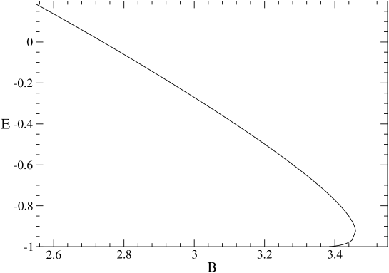
Figure 2: Spectrum of the Klein-Gordon equation with $B$ between 2.54 and 3.45, $D=$ 0.86, $k=1$, $a=1$

We observe that in the situation described by Fig. (2), we obtain complex energy values for values of $B$ larger than the turning point $B=3.459$ (for this critical value the energy reaches the value $E=-0.92355$ and starts generating antiparticle bound states coming form the negative energy continuum). The associated eigenstate with this critical value has a zero norm in the sense of Ref BL:79 and Eq. (8). Below this critical value, the norm associated with the energy states remains negative and above this value it becomes positive.

For the situation described in Fig. (3) the energy $E$ reaches the value $E=-1$ for $B=9.1305$. In this case, the norm remains always positive. Beyond this critical value, there is an embedding process into the negative energy continuum.

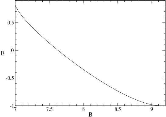
Figure 3: Spectrum of the Klein-Gordon equation with $B$ between 6.99 and 9.13, $D=-11$, $k=10$, $a=0.6$

Making $k^{2}=E^{2}-m^{2}\equiv-\kappa^{2}$ in Eq. (7), we obtain $u_{f}(r)$ for the $s$ waves belonging to the continuum:

$$u^{c}_{r}(r)=C_{3}\,\frac{e^{i\left(-\kappa\,r+\delta\right)}}{r}$$ (9)

Repeating the procedure applied in the derivation of the eigenvalue equation with this new function we obtain an expression giving $\delta$ in terms of the energy, that is: $\delta\left(E\left(B,D,k,a\right)\right)$.

We now show the figures depicting $\delta\left(E\left(B,D,k,a\right)\right)$ for the cases described by Fig. (2) and Fig. (3) respectively.

In order for a resonance to exist the Wigner time delay must be positive. This is defined as

$$\tau=2\frac{d\delta}{dE},$$ (10)

so the phase shift must increase through $\pi/2$ with the energy. A decrease in the phase shift as the energy increases through $\pi/2$ produces an unphysical negative time delay Kamke , and does not constitute a resonance.

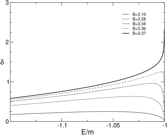
Figure 4: Phase shift associated with the energy spectrum described in Fig. (2).

In Fig. (4) the curves tend to the asymptotic value $\pi/2$ for $\delta$ without reaching it; here we are in the presence of an attempt of formation of a bound state but the potential is not strong enough in order to support such a state. Nevertheless, we are not in the presence of a resonance since, for this situation, the Wigner time delay EW:55 is not positive. Fig. (4) shows that the appearance of a antiparticle state, phenomenon that takes place for the value $B\approx 3.459$, and that does not represent a dramatic change in the phase shift (a jump to $\delta=\pi$) that experiences a bound state crossing through $E=-1$.

In Fig. (5) the curves overpass the value $\pi/2$, reaching the value of $\pi$ for $\delta$, finding us in this way in the presence of a resonance for the values of $B$ shown in the figure. It is worth noticing that in this case the Wigner time delay is positive. The phase shifts experiences a drastic change in the resonant value.

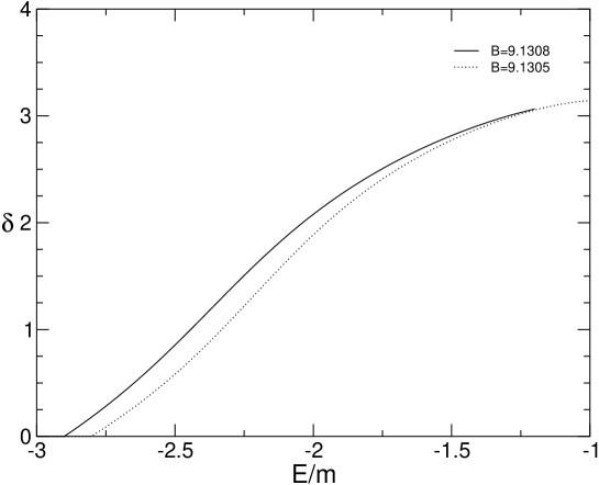
Figure 5: Phase shift associated with the energy spectrum described in Fig. (3)

From Fig (2) and Fig. (3) we observe that both curves possess different concavity, being positive in the resonant-embedding regime and negative when the Schiff-Snyder effect is present. This behavior is analogous to the one observed for $p$ states in the scalar well BL:79 . It is worth mentioning that both the Schiff-Snyder and the embedding effect depend on the sign of the shape constant $D$ in the potential $V(r)$ (2).

We have shown evidence of a short-range potential that for $s$ waves exhibit Fig. (3) and Fig. (5) show evidence that, for $s$ waves, there is a resonant behavior for a class of short range potentials, with $D<0$ in Eq. (2), this result is, based on the results reported in Ref.VP:71 , new and unexpected.

- (1) W. Greiner, B. Müller J and Rafelski Quantum Electrodynamics of Strong Fields (Springer, Berlin 1985)
- (2) W. Greiner, Relativistic Quantum Mechanics, Wave equations (Springer, 1990)
- (3) S. A. Fulling, Aspects of Quantum Field Theory in Curved Space-Time (Cambridge UP, Cambridge 1991).
- (4) V. R. Khalilov, and C. L. Ho, Phys. Rev. D. 60 033003 (1999).
- (5) V. R. Khalilov Electrons in strong magnetic fields. (Energoatomizdat, Moscow 1988)
- (6) W. Fleischer, and G. Soff, Z. Naturforsch 39A, 703 (1984).
- (7) M. Bawin and J. P. Lavine, Lett. Nuovo Cimento 26, 586 (1979).
- (8) L. I. Schiff, H. Snyder and J. Weinberg, Phys. Rev. 57, 315 (1940).
- (9) H. Snyder and J. Weinberg, Phys. Rev. 57, 307 (1940).
- (10) J. Rafelski, L. P. Fulcher and A. Klein, Phys. Rep. C 38, 227 (1978).
- (11) R. G. Newton, Scattering Theory of Waves and Particles (Springer-Verlag, Berlin 1982).
- (12) E. Wigner, Phys. Rev. 98, 145 (1955).
- (13) V. S. Popov, Sov. Phys. JETP 32, 526 (1971).
- (14) D. Kamke, Am. J. Phys. 53, 274 (1985).