Discreteness and its effect on the water-wave turbulence.

Abstract

We perform numerical simulations of the dynamical equations for free water surface in finite basin in presence of gravity. Wave Turbulence (WT) is a theory derived for describing statistics of weakly nonlinear waves in the infinite basin limit. Its formal applicability condition on the minimal size of the computational basin is impossible to satisfy in present numerical simulations, and the number of wave resonances is significantly depleted due to the wavenumber discreteness. The goal of this paper will be to examine which WT predictions survive in such discrete systems with depleted resonances and which properties arise specifically due to the discreteness effects. As in [1, 2, 3], our results for the wave spectrum agree with the Zakharov-Filonenko spectrum predicted within WT. We also go beyond finding the spectra and compute probability density function (PDF) of the wave amplitudes and observe an anomalously large, with respect to Gaussian, probability of strong waves which is consistent with recent theory [4, 5]. Using a simple model for quasi-resonances we predict an effect arising purely due to discreteness: existence of a threshold wave intensity above which turbulent cascade develops and proceeds to arbitrarily small scales. Numerically, we observe that the energy cascade is very “bursty” in time and is somewhat similar to sporadic sandpile avalanches. We explain this as a cycle: a cascade arrest due to discreteness leads to accumulation of energy near the forcing scale which, in turn, leads to widening of the nonlinear resonance and, therefore, triggering of the cascade draining the turbulence levels and returning the system to the beginning of the cycle.

1 Introduction

Normal state of the sea surface is chaotic with a lot of waves at different scales propagating in random directions. Such a state is referred to as Wave Turbulence (WT). Theory of WT was developed by finding a statistical closure based on the small nonlinearity and on the Wick splitting of the Fourier moments, the later procedure is often interpreted as closeness of statistics to Gaussian or/and to phase randomness (the two are not the same, see [6, 4, 5]). This closure yields a wave-kinetic equation (WKE) for the waveaction spectrum. Such WKE for the surface waves was first derived by Hasselmann [7]. A significant achievement in WT theory was to realize that the most relevant states in WT are energy cascades through scales similar to the Kolmogorov cascades in Navier-Stokes turbulence, rather than thermodynamic equilibria as in the statistical theory of gases. This understanding came when Zakharov and Filonenko found an exact power-law solution to WKE which is similar to the famous Kolmogorov spectrum [8].

Numerical simulation of the moving water surface is a challenging problem due to a tremendous amount of computing power required for computing weakly nonlinear dispersive waves. This arises due to presence of widely separated spatial and time scales. As will be explained below, the weaker we take nonlinearity, the larger we should take the computational box in order to overcome the $k$-space discreteness and ignite wave resonances leading to the energy cascade through scales. In order to maximize the inertial range, one tries to force at the lowest wavenumbers possible, but without forgetting that the forcing should be strong enough for the resonance broadening to overcome the discreteness effect. But nonlinearity tends to grow along the energy cascade toward high $k$’s [9, 10] and, therefore, the forcing at low wavenumbers should not be too strong for the nonlinearity to remain weak throughout the inertial range. A simple estimate [11] says that for the resonant interactions to be fully efficient, one must have a $N\times N$ computational box with the number of modes $N$ related to the mean surface angle $\alpha$ as

$$N>1/\alpha^{4}.$$

Thus, for small enough nonlinearity $\alpha\sim 0.1$ one must have at least $10000\times 10000$ resolution which is far beyond present computational capacity. Thus, in none of the existing numerical experiments, nor in near future, the formal applicability conditions of WT can be realized. On the other hand, a small fraction of the resonances can be activated at levels of nonlinearity which is much less than in the above estimate and this reduced set of resonant modes can, in principle, be sufficient to carry the turbulent cascade through scales. In this paper we estimate the minimal resonance broadening which is sufficient to generate the cascade.

It is necessary to examine which of the WT predictions survive beyond the formal applicability conditions when the cascade is carried by a depleted set of resonant modes, and which specific features arise due to such resonance depletion.

As in other recent numerical experiments [1, 2, 3], here we observe formation of a spectrum consistent with the ZF spectrum corresponding to the direct energy cascade. For this, the resonance broadening at the forcing scale should be maintained at about an order of magnitude larger than the minimal level necessary for triggering the cascade. Further, in agreement with more recent WT predictions about the higher-order statistics [4, 5], we observe an anomalously high (with respect to Gaussian) probability of the large-amplitude waves. Also in agreement with recent WT findings [5], we observe a buildup of strong correlations of the wave phases $\phi_{k}$ whereas the factors $e^{i\phi_{k}}$ remain de-correlated.

There are also distinct features arising due to discreteness. We analyze them by exploiting the two-peak structure of the time-Fourier transform at each $k$: a dominant peak at (very close to) linear frequency $\omega_{k}$, and a weaker one with a frequency approximately equal to $2\omega_{k/2}$. The second peak is a contribution of the $k/2$-mode in the nonlinear term of the canonical transformation relating the normal variable and the observables (e.g. surface elevation). In fact, the nature of the second frequency peak is quite well understood in literature and it has even been used for remote sensing of vertical sheer by VHF frequency radars [13]. In absence of nonlinearity one would observe only the first but not the second peak and, therefore, one can quantify the nonlinearity level as the ratio of the amplitudes of these two peaks. When the second peak becomes stronger than the first one, the wave phase experiences a rapid and persistent monotonic change. Detecting such phase “runs” gives an interesting picture of the nonlinear activity in the 2D $k$-space. In particular, we notice a “bursty” nature of the energy cascade resembling sandpile avalanches. Possible explanation of such behavior is the following. When nonlinearity is weak, there is no wave-wave resonances, consequently there is no effective energy transfer, and system behaves like “frozen turbulence” (term introduced in [14] for the capillary wave turbulence). Energy generated at the forcing scale will accumulate near this scale and the nonlinearity will grow. When resonance broadening gets wide enough, so that the resonances are not inhibited by discreteness, the nonlinear wave-wave energy transfer starts, which diminishes nonlinearity and subsequently “arrests” resonances. Thus the system oscillates between having almost linear oscillations with stagnated energy and occasional avalanche-like discharges.

2 Equations for the free surface

Let us consider motion of a water volume of infinite depth embedded in gravity and bounded by a surface separating it from air at height $z=\eta({\bf x},t)$ where ${\bf x}=(x,y)$ is the horizontal coordinate. Let the velocity field be irrotational, ${\bf u}=\nabla\Phi$, so that the incompressibility condition becomes

$$\Delta\Phi=0,\hskip 28.45274pt\hbox{for\;\;}z<\eta({\bf x},t).$$ (1)

Rate of change of the surface elevation must be equal to the vertical velocity of the fluid particle on this surface, which gives

$$D_{t}\eta=\partial_{z}\Phi,\hskip 28.45274pt\hskip 28.45274pt\hbox{for\;\;}z=\eta({\bf x},t),$$ (2)

where $D_{t}=\partial_{t}+{\bf u}\cdot\nabla_{\perp}$ is the material time derivative. The second condition at the surface arises from the Bernoulli equation in which pressure is taken equal to its atmospheric value. This condition gives

$$\partial_{t}\Phi+{1\over 2}|\nabla\Phi|^{2}=-g\eta,\hskip 28.45274pt\hskip 28.45274pt\hbox{for\;\;}z=\eta({\bf x},t),$$ (3)

where $g$ is the free-fall acceleration.

Although equations (2) and (3) involve only two-dimensional coordinate ${\bf x}$, the system remains three-dimensional due to the 3D equation (1). One can transform these equations to a truly 2D form by assuming that the surface deviates from its rest plane only by small angles and by truncating the nonlinearity at the cubic order with respect to the small deviations. This procedure yields the following dynamical equations (see e.g. [17, 15]):

$$\eta_{t} = \mathbf{\Gamma}\left[\Psi\right]$$

$$-\varepsilon\left(\mathbf{\Gamma}\left[\mathbf{\Gamma}\left[\Psi\right]\eta\right]+\nabla_{\bot}\cdot\left[\left(\nabla_{\bot}\Psi\right)\eta\right]\right)$$

$$+\varepsilon^{2}\left(\Gamma\left[\mathbf{\Gamma}\left[\mathbf{\Gamma}\left[\Psi\right]\eta\right]\eta\right]+\frac{1}{2}\Gamma\left[\left(\Delta_{\bot}\Psi\right)\eta^{2}\right]+\frac{1}{2}\Delta_{\bot}\left(\mathbf{\Gamma}\left[\Psi\right]\eta^{2}\right)\right),$$

$$\Psi_{t} = -g\eta$$

$$-\varepsilon\frac{1}{2}\left(\left|\nabla_{\bot}\Psi\right|^{2}-\left(\Gamma[\Psi]\right)^{2}\right)$$

$$-\varepsilon^{2}\Gamma[\Psi]\left(\mathbf{\Gamma}\left[\mathbf{\Gamma}\left[\Psi\right]\eta\right]+\left(\Delta_{\bot}\Psi\right)\eta\right),$$

where

$$\Psi=\Phi|_{z=\eta({\bf x},t)},$$ (6)

and $\Gamma$ is the Gilbert transform which in the Fourier space corresponds to multiplication by $k=|{\bf k}|$, i.e.

$$\Gamma\left[f\right](\mathbf{x},t)=\frac{1}{2\pi}\int k\widehat{f}(\mathbf{k},t)e^{i\mathbf{k}\cdot\mathbf{x}}d\mathbf{k}.$$

Here, we have the following convention for defining the Fourier transform

$$\widehat{f}(\mathbf{k})={1\over 2\pi}\int e^{i(\mathbf{k}\cdot\mathbf{x})}f(\mathbf{x})\,d\mathbf{k}.$$ (7)

In equations (2) and (2), we rescaled variables $\eta$ and $\Psi$ to make them order one, so that the nonlinearity smallness is now in a formal parameter $\epsilon\ll 1$.

Truncated equations (2) and (2) will be used for our numerical simulations. They have a convenient form for the pseudo-spectral method which computes evolution of the Fourier modes but switches back to the coordinate space for computing the nonlinear terms. However, for theoretical analysis these equations have to be diagonalised in the $k$-space and a near-identity canonical transformation must be applied to remove the nonlinear terms of order $\epsilon$ since the gravity wave dispersion $\omega=\sqrt{gk}$ does not allow three-wave resonances. The resulting equation is also truncated at $\epsilon^{2}$ order and it is called the Zakharov equation [17, 18, 19, 16],

$$i\dot{a}_{l}=\epsilon^{2}\sum_{\alpha\mu\nu}{W^{l\alpha}_{\mu\nu}}\bar{a}_{\alpha}a_{\mu}a_{\nu}e^{i\omega^{l\alpha}_{\mu\nu}t}\delta^{l\alpha}_{\mu\nu},$$ (8)

where $\omega^{l\alpha}_{\mu\nu}=\omega_{l}+\omega_{\alpha}-\omega_{\mu}-\omega_{\nu}$, $\omega_{l}=\sqrt{gk_{l}}$ is the frequency of mode ${\bf l}$ ($\;{\bf l}\in{\cal Z}^{2}$), ${\bf k}_{l}=2\pi{\bf l}/L$ is the wavenumber, $L$ is the box size and $k_{l}=|{\bf k}_{l}|$. Here, $a_{l}$ is the wave action variable in the interaction representation, $a_{l}=e^{i\omega_{l}t}b_{l}$ where $b_{l}$ is a normal variable,

$$b_{l}=\sqrt{\omega_{l}\over 2k_{l}}\eta_{l}+i\sqrt{k_{l}\over 2\omega_{l}}\Psi_{l}+0(\epsilon).$$ (9)

Here, $0(\epsilon)$ terms appear because of the near-identity canonical transformation needed to remove the quadratic terms from the evolution equations [17, 21, 16, 20, 18, 19]. Expression for the interaction coefficient $W^{l\alpha}_{\mu\nu}$ is lengthy and can be found in [21].

Zakharov equation is of fundamental importance for theory and it is also sometimes used for numerics. However, in our work we choose to compute equations (2) and (2) because this allows us to use the standard trick of pseudo-spectral methods via computing the nonlinear term in the real thereby accelerating the code.

3 Statistical Quantities in Wave Turbulence

Let us consider a wavefield in a periodic square basin of side $L$ and let the Fourier representation of this field be $a_{l}(t)$ where index ${\bf l}{\in}{\cal Z}^{2}$ marks the mode with wavenumber ${\bf k}_{l}=2\pi{\bf l}/L$ on the grid in the $2$-dimensional Fourier space. Discrete $k$-space is important for formulating the statistical problem. For simplicity let us assume that there is a cut-off wavenumber $k_{max}$ so that thee is no modes with wavenumber components greater than $k_{max}$, which is always the case in numerical simulation. In this case, the total number of modes is $N=(k_{max}/\pi L)^{2}$ and index ${\bf l}$ will only take values in a finite box, ${\bf l}\in{\cal B}_{N}\subset{\cal Z}^{2}$ which is centered at 0 and all sides of which are equal to $N^{1/2}$. To consider homogeneous turbulence, the large box (i.e. continuous $k$) limit, $N\to\infty$, will have to be taken later.

Let us write the complex $a_{l}$ as $a_{l}=A_{l}\psi_{l}$ where $A_{l}$ is a real positive amplitude and $\psi_{l}$ is a phase factor which takes values on ${\cal S}^{1}$, a unit circle centered at zero in the complex plane. The most general statistical object in WT [5] is the $N$-mode joint PDF ${\cal P}^{(N)}$ defined as the probability for the wave intensities $A_{l}^{2}$ to be in the range $(s_{l},s_{l}+ds_{l})$ and for the phase factors $\psi_{l}$ to be on the unit-circle segment between $\xi_{l}$ and $\xi_{l}+d\xi_{l}$ for all ${\bf l}\in{\cal B}_{N}$.

The fundamental statistical property of the wavefield in WT is that all the amplitudes $A_{l}$ and phase factors $\psi_{l}$ are independent statistical variables and that all $\psi_{l}$’s are uniformly distributed on ${\cal S}^{1}$. This kind of statistics was introduced in [6, 4, 5] and called “Random Phase and Amplitude” (RPA) field. In terms of the PDF, we say that the field $a$ is of RPA type if it can be product-factorized,

$${\cal P}^{(N)}\{s,\xi\}={1\over(2\pi)^{N}}\prod_{{\bf l}\in{\cal B}_{N}}P^{(a)}_{l}(s_{l}),$$ (10)

where $P^{(a)}_{l}(s_{l})$ is the one-mode PDF for variable $A_{l}^{2}$.

Note that in this formulation the distributions of $A_{l}$ remain unspecified and, therefore, the amplitudes do not have to be deterministic (as in earlier works using RPA) nor do they have to correspond to Gaussianity,

$$P^{(a)}_{l}(s_{l})={1\over n_{l}}\,\exp{(-s_{l}/n_{l})}$$ (11)

where $n_{l}=\langle s_{l}\rangle$ is the waveaction spectrum.

Importantly, RPA formulation involves independent phase factors $\psi=e^{i\phi}$ and not phases $\phi$. Firstly, the phases would not be convenient because the mean value of the phases is evolving with the rate equal to the nonlinear frequency correction [5]. Thus one could not say that they are “distributed uniformly from $-\pi$ to $\pi$”. Moreover the mean fluctuation of the phase distribution is also growing and they quickly spread beyond their initial $2\pi$-wide interval [5]. But perhaps even more important, it was shown in [5] that $\phi$’s build mutual correlations on the nonlinear timescale whereas $\psi$’s remain independent. In the present paper we are going to check this theoretical prediction numerically by directly measuring the properties of $\phi$’s and $\psi$’s.

In [6, 4] RPA was assumed to hold over the nonlinear time. In [5] this assumption was examined a posteriori, i.e. based on the evolution equation for the multi-point PDF. Note that only the phase randomness is necessary for deriving this equation, whereas both the phase and the amplitude randomness are required for the WT closure for the one-point PDF or the kinetic equation for the spectrum. This fact allows to prove that, if valid initially, the RPA properties survive in the leading order in small nonlinearity and in the large-box limit [5]. Such an approximate leading-order RPA is sufficient for the WT closure.

4 Theoretical WT predictions

When the wave amplitudes are small, the nonlinearity is weak and the wave periods, determined by the linear dynamics, are much smaller than the characteristic time at which different wave modes exchange energy. In the other words, weak nonlinearity results in a timescale separation and this fact is exploited in WT to describe the slowly changing wave statistics by averaging over the fast linear oscillations.

4.1 Evolution equations for the PDF’s, moments and spectrum.

In [5] the following equation for for the $N$-mode PDF was obtained for the four-wave systems,

$$\dot{\cal P}={\pi{\epsilon}^{2}}\int|W^{jl}_{nm}|^{2}\delta(\tilde{\omega}^{jl}_{nm})\delta^{jl}_{nm}\left[{\delta\over\delta s}\right]_{4}\left(s_{j}s_{l}s_{m}s_{n}\left[{\delta\over\delta s}\right]_{4}{\cal P}\right)\,d{\bf k}_{j}d{\bf k}_{l}d{\bf k}_{m}d{\bf k}_{n},$$ (12)

where

$$\left[{\delta\over\delta s}\right]_{4}={\delta\over\delta s_{j}}+{\delta\over\delta s_{l}}-{\delta\over\delta s_{m}}-{\delta\over\delta s_{n}}.$$ (13)

Here $N\to\infty$ limit has already been taken and ${\delta\over\delta s_{j}}$ means the variational derivative. Using this equation, one can prove that RPA property holds over the nonlinear time, i.e. the $N$-mode PDF remains of the product factorized form with accuracy sufficient for the WT closures to work [5]. Using RPA, we get for the one-point marginals [5],

$${\partial P_{a}\over\partial t}+{\partial F\over\partial s_{j}}=0,$$ (14)

with $F$ is a probability flux in the s-space,

$$F=-s_{j}(\gamma P_{a}+\eta_{j}{\delta P_{a}\over\delta s_{j}}),$$ (15)

where

$$\eta_{j} = 4\pi\epsilon^{2}\int|W^{jl}_{nm}|^{2}\delta^{jl}_{nm}\delta(\omega^{jl}_{nm})n_{l}n_{m}n_{n}\,d{{\bf k}_{l}}d{{\bf k}_{m}}d{{\bf k}_{n},}$$ (16)

$$\gamma_{j} = 4\pi\epsilon^{2}\int|W^{jl}_{nm}|^{2}\delta^{jl}_{nm}\delta(\omega^{jl}_{nm})\Big{[}n_{l}(n_{m}+n_{n})-n_{m}n_{n}\Big{]}\,d{{\bf k}_{l}}d{{\bf k}_{m}}d{{\bf k}_{n}.}$$ (17)

Here we introduced the wave-action spectrum,

$$n_{j}=\langle A_{j}^{2}\rangle.$$ (18)

From (14) we get the following equation for the moments $M^{(p)}_{j}=\langle A_{j}^{2p}\rangle$:

$$\dot{M}^{(p)}_{j}=-p\gamma_{j}M^{(p)}_{j}+p^{2}\eta_{j}M^{(p-1)}_{j}.$$ (19)

which, for $p=1$ gives the standard wave kinetic equation (WKE),

$$\dot{n}_{j}=-\gamma_{j}n_{j}+\eta_{j}.$$ (20)

4.2 Preservation of the RPA property.

Validity of the WT theory relies on persistence of the RPA property of the wavefield over the nonlinear evolution time. Such persistence was demonstrated in [5] based on the evolution equation for the multi-mode PDF, where the product factorization of PDF was shown to hold with an accuracy sufficient for the WT closure. It was also emphasized in [5] that RPA must use independent phase factors $\psi_{k}$ rather than the phases $\phi_{k}$ independence of which does not survive over the nonlinear time. The theoretical prediction of persistent independence of $A_{k}$’s and $\psi_{k}$’s and about the growth of correlations of $\phi_{k}$’s will be checked in this paper numerically.

Further, the WT approach predicts that the mean value of the phase grows with a rate given by the nonlinear frequency correction and that the r.m.s. fluctuation of the phase also grows in time [5]. In this paper we will see that in reality the time evolution of the phase is more complicated than this WT prediction: the phase exhibits quasi-periodic fluctuations intermittent by rare “phase runs”, - monotonic changes over several linear periods by large values which can significantly exceed $2\pi$.

4.3 Steady state solutions.

Steady power-law solutions of WKE which correspond to a direct cascade of energy and an inverse waveaction cascade are,

$$n(k) = C_{1}P^{1/3}k^{-4}$$ (21)

$$n(k) = C_{2}Q^{1/3}k^{-23/6},$$ (22)

where $P$ and $Q$ are the energy and the waveaction fluxes respectively and $C_{1}$ and $C_{2}$ are constants, and $k=|{\bf k}|$. The first of these solutions is the famous ZF spectrum [8] and it has a great relevance to the small-scale part of the sea surface turbulence. It has been confirmed in a number of recent numerical works [1, 2, 3], but we will also confirm it in our simulation.

Now, let us consider the steady state solutions for the one-mode PDF. Note that in the steady state $\gamma/\eta=n$ which follows from WKE (20). Then, the general steady state solution to (14) is

$$P=\hbox{const}\,\exp{(-s/n)}-({F}/{\eta})Ei({s}/{n})\exp{(-s/n)},$$ (23)

where $Ei(x)$ is the integral exponential function. At the tail $s\gg n_{k}$ we have

$$P\to-\frac{F}{s\gamma}$$ (24)

if $F\neq 0$. The $1/s$ tail decays much slower than the exponential (Rayleigh) part and, therefore, it describes strong intermittency. On the other hand, $1/s$ tail cannot be infinitely long because otherwise the PDF would not be normalizable. As it was argued in [5], the $1/s$ tail should with a cutoff because the WT description breaks down at large amplitudes $s$. This cutoff can be viewed as a wavebreaking process which does not allow wave amplitudes to exceed their critical value, $P(s)=0$ for $s>s_{nl}$.

Relation between intermittency and a finite flux in the amplitude space was observed numerically also for the Majda-Mc-Laughlin-Tabak model by Rumpf and Biven [22].

5 Resonant interaction in discrete $k$-space

Importance of the $k$-space discreteness for weakly nonlinear waves in finite basins were realized by Kartashova [23] and it was later discussed in a number of papers, [14, 28, 29, 30]. Nonlinear wave interactions crucially depend on the sort of resonances the dispersion relation allows. The dispersion relation of the surface gravity waves is concave and hence it forbids three-wave interactions, so that the dominant process is four-wave. Resonant manifold is defined by resonant conditions $\mathbf{k}+\mathbf{k}_{1}=\mathbf{k}_{2}+\mathbf{k}_{3}$, $\omega_{\mathbf{k}}+\omega_{\mathbf{k}_{1}}=\omega_{\mathbf{k}_{2}}+\omega_{\mathbf{k}_{3}}$ or, substituting $\omega_{\mathbf{k}}=\sqrt{gk}$,

$$\mathbf{k}+\mathbf{k}_{1} = \mathbf{k}_{2}+\mathbf{k}_{3}$$

$$\sqrt{k}+\sqrt{k_{1}} = \sqrt{k_{2}}+\sqrt{k_{3}}$$ (25)

The problem of finding exact resonances in discrete $k$-space was first formulated by Kartashova [23] who gave a detailed classification of for some types of waves, e.g. Rossby waves. For the deep-water gravity waves, Kartashova only considered symmetric solutions, i.e. of the form $k=k_{2},k_{1}=k_{3}$ (or $k=k_{3},k_{1}=k_{2}$). Interestingly, there appear to be also asymmetric solutions,

Solutions for collinear quartets and the tridents are easy to find by rewriting the resonant conditions (25) as polynomial equations (appropeiately re-arranging and taking squares of the equations) and using rational parametrisations of their solutions. This way we get the following family of the collinear quartets [24],

$$\mathbf{k}=(a,0),\;\;\mathbf{k}_{1}=(b,0),\;\;\mathbf{k}_{2}=(c,0),\;\;\mathbf{k}_{3}=(d,0)$$

with

$$a=m^{2}(m+n)^{2},\;\;b=n^{2}(m+n)^{2},\;\;c=-m^{2}n^{2},\;\;d=(m+n)^{4}+m^{2}n^{2},$$

where $m$ and $n$ are natural numbers, and “tridents”,

$$\mathbf{k}=(a,0),\;\;\mathbf{k}_{1}=(-b,0),\;\;\mathbf{k}_{2}=(c,d),\;\;\mathbf{k}_{3}=(c,-d)$$

with

$$a=(s^{2}+t^{2}+st)^{2},\;\;b=(s^{2}+t^{2}-st)^{2},\;\;c=2st(s^{2}+t^{2}),\;\;d=s^{4}-t^{4},$$

where $s$ and $t$ are integers. Both of these classes can be easily extended by re-scaling, i.e. multiplying all four vectors by an integer. Even more solutions can be obtained via rotation by an angle with rational-valued cosine (this gives a new rational solution) and further re-scaling (to obtain integer solution out of the rational one).

There are other, rather rare, exact nontirvial resonances, for example one provided to us by Kartashova [25]:

$${\bf k}=(495,90),\ {\bf k_{1}}=(64,128),\ {\bf k_{2}}=(359,118),\ {\bf k_{3}}=(200,100).$$

The complete investigation of the exact resonance types and their respective roles is a facinating subject of future work).

Note that the interactions coefficient vanishes on the collinear quartets [27] and, therefore, these quartets do not contribute into the turbulence evolution. Secondly, there appears to be much more symmetric quartets than tridents, so the later are relatively unimportant for the nonlinear dynamics too.

Because of nonlinearity, the wave resonances have a finite width. Even though this width is small in weakly nonlinear systems, it may be sufficient for activating new mode interactions on the $k$-space grid and thereby trigger the turbulent cascade through scales. Such quasi-resonances can be roughly modeled through $\mathbf{k}_{1}+\mathbf{k}_{2}=\mathbf{k}_{3}+\mathbf{k}_{4}$, $\left|\omega_{\mathbf{k}_{1}}+\omega_{\mathbf{k}_{2}}-\omega_{\mathbf{k}_{3}}-\omega_{\mathbf{k}_{4}}\right|<\delta$, where $\delta$ describes the resonance broadening. Figure 1 shows quasi-resonant generations of modes on space $[-64,64]^{2}$, where initially (generation 1) only modes in the ring $6<k<9$ were present (as in our numerical experiment). With broadening of the resonant manifold smaller than the critical $\delta_{crit}\sim 1.4\ast 10^{-5}$, a finite number of modes outside the initial region get excited due to exact resonances (generation 2) but there are no quasi-resonances to carry energy to outer regions in further generations. If broadening is larger than critical, energy cascades infinitely. Contrary to the the case of capillary waves where quasi-resonant cascades die out if broadening is not large enough [28], in the case presented here quasi-resonant cascades either do not happen at all (if $\delta<\delta_{\rm crit}$) or they spread through the wavenumber space infinitely (if $\delta>\delta_{\rm crit}$), as happens on Figure (1).

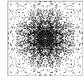
Figure 1: Quasi-resonant generations of modes on Fourier space $[-64,64]^{2}$, where initially (generation 1) only modes in the ring $6<k<9$ were present. Each next generation consists of the union of the modes of the current generation and the new modes which satisfy the quasi-resonance condition with the modes of the current generation. Here the value of the broadening is slightly above $\delta_{crit}$

6 Numerical simulation

Numerical simulations presented in this work were performed on a single-processor workstation (2.5GHz, 1Gb RAM). We performed a direct numerical simulation, integrating the dynamical equations of motion (2) and (2) using pseudo-spectral method with resolution of $256\times 256$ wavenumbers. Numerical integrator used for advancing in time was RK7(8) presented in [31]. Time step was $\frac{T_{min}}{35}$ where $T_{min}$ is the period of the shortest wave on the axis. Approximate processor time for this work was 4.5 weeks.

In our numerical experiment, we force the system in the $k$-space ring $k_{*}<k<k^{*}$ with $k_{*}=6$ and $k^{*}=9$. This ring is located at the low wavenumber part of the $k$-space in order to generate energy cascade toward large $k$’s, but we deliberately avoid forcing even longer waves ($k<6$) because our experience shows that this would lead to undesirable strong anisotropic effects. In the ring, we fix the shape to coincide with the ZF spectrum, $<|a_{\mathbf{k}}(t)|^{2}>\sim k^{-4}$, and hence we set $|\eta_{\mathbf{k}}|\sim k^{-7/4}$, $|\Psi_{\mathbf{k}}|\sim k^{-9/4}$. These fixed amplitudes were then multiplied by random phase factors. Thus, surface $\eta_{\mathbf{k}}$ and velocity potential $\Psi_{\mathbf{k}}$ were set to $2\pi^{3}\,e^{i\theta_{\mathbf{k}}}\ast k^{\alpha_{\mathbf{k}}}$, where $\theta_{\mathbf{k}}$ were uniformly distributed in $[0,2\pi]$ and

$$\alpha_{k}=x\left\{\begin{array}[]{cc}\left[1+\left(\frac{k_{\ast}-k}{k^{\ast}}\right)^{2}\right]^{3/4}&\hbox{if}\;k\in\left(0,k_{\ast}\right)\\ 1&\hbox{if}\;k\in[k_{\ast},k^{\ast}]\\ \left(\frac{k}{k^{\ast}}\right)^{3/4}&\hbox{if}\;k\in\left(k^{\ast},\frac{N}{2}\right)\end{array}\right\}$$

where $x=-7/4$ for the surface and $x=-9/4$ for velocity potential. Damping was applied in both small and large wavenumber regions. At small wavenumbers inside the forcing ring, we applied an adaptive damping to prevent formation of undesirable “condensate” which could spoil isotropy and locality of scale interactions. At large wavenumbers, damping is needed to absorb the energy cascade and, therefore, to avoid “bottleneck” spectrum accumulation near the cutoff wavenumber. In our simulations, we implemented the damping as a low-pass filter $\gamma_{\mathbf{k}}$ applied to the $k$-space variables at each time step. The damping function had the form

$$\gamma_{\mathbf{k}}=\left\{\begin{array}[]{cc}5\left(k-6\right)^{3/2}&k<6\\ 0&k\in\left[6,64\right]\\ 0.028\left(k-64\right)^{2}&k>64\end{array}\right\}$$

Nonlinearity parameter was set to $\varepsilon=2\cdot 10^{-2}$, which is a sufficient value to produce a resonance broadening for supporting energy cascade.

7 Results

7.1 Spectrum

Measuring the spectrum has by far dominated WT studies because this is the most basic and robust theoretical object and because this quantity is easier to observe experimentally that more subtle statistical quantities. For the surface gravity waves, the WT prediction about the energy cascade spectrum have been confirmed in several recent numerical studies [2, 3, 1]. Here, we also start by presenting the spectrum. Figure 2 shows the spectrum at $t=300T_{p}$ at $t=2000T_{p}$, where $T_{p}$ is period of the slowest mode ($k=10$). The obtained spectrum is in agreement with the $k^{-4}$ shape predicted by WT theory in the inertial range, and this serves as a validation of our code. Our subsequent statistical measurements will be made at the time where this steady state spectrum has already got established.

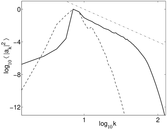
Figure 2: Waveaction spectrum of waves. Dashed and solid lines show spectra after 300 and 2000 periods of mode $k=10$. The straight line corresponds to the ZF spectrum ($-4$ slope).

7.2 Wave-amplitude probability density function and its moments

Now we consider the PDF of amplitudes for which predictions where made recently within the WT approach. To measure the PDF of amplitudes $\left|a_{\mathbf{k}}(t)\right|^{2}$, we set two radial regions in $\mathbf{k}$-space $k_{15}=[13,17],$ and $k_{35}=[33,37]$. These regions were inside the inertial range and had well mixed phases and amplitudes since the experiment was done after performing 2000 rotations of the peak mode. We looked at the time-span of approximately 855 rotations of modes $k=15$ or 1230 rotations of modes $k=35$ and collected amplitudes of all modes from these three regions. The number of amplitudes collected was over 1.1 million in region $k_{15}$ and over 2.1 million in region $k_{35}$.

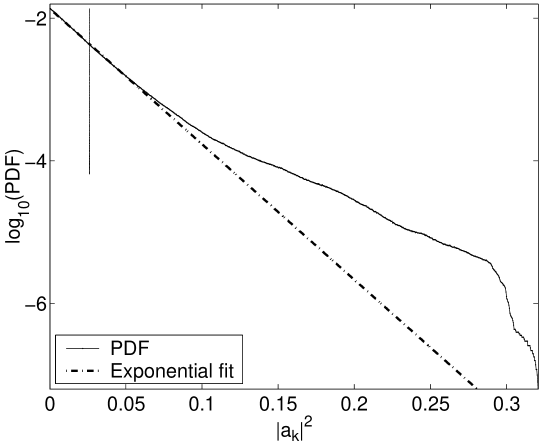
Figure 3: Probability density function for the amplitude $|a_{k}|^{2}$ with $k\in[13,17]$. The linear fit is shown based on the slope of the low-amplitude part (the Gaussian core). The vertical straight line marks the mean value (spectrum) $n_{k}=\langle|a_{k}|^{2}\rangle$.

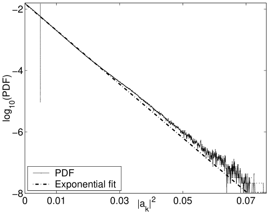
Figure 4: Probability density function for the amplitude $|a_{k}|^{2}$ with $k\in[33,37]$. Same notations as in Figure 3.

Figure 3 shows a log-plot of the PDF the amplitude $A_{k}^{2}$ in $k_{15}$ and an exponential fit of its low-amplitude part. One can see intermittency, i.e., an anomalously large probability of strong waves. We can also see that this discrepancy from Gaussianity happens in the tail, i.e. well below the mean amplitude value $s=n_{k}$. While the PDF tail in not long enough for drawing decisive conclusions about realization of the theoretically predicted $1/s$ scaling, it certainly gives a conclusive evidence that the probabilities of large amplitudes are orders of magnitude higher than in Gaussian turbulence. Figure 4 shows the PDF of $A_{k}^{2}$ in $k_{35}$. We can see some non-Gaussianity in $k_{35}$ as well, although much less than in $k_{15}$. Similar conclusion that the gravity wave turbulence is more intermittent at low rather than high wavenumbers was reached on the basis of numerical simulations in [3].

Deviations from Gaussianity can be also seen in figure 5 which shows ratio of the moments $M^{(p)}=\langle|a|^{2p}\rangle$ to their values in Gaussian turbulence, $n\,p!$. Again, we can see that such deviations are greater at the small-$k$ part of the inertial range.

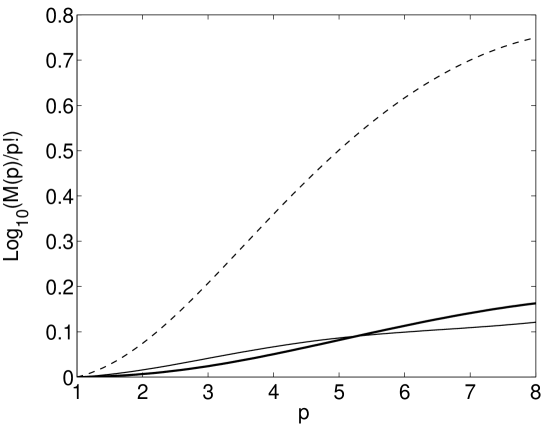
Figure 5: Ratio of the moments $M^{(p)}=\langle|a|^{2p}\rangle$ to their values in Gaussian turbulence, $n\,p!$, for $k\in[13,17]$ (dashed line), $k\in[23,27]$ (thin solid line) and $k\in[33,37]$ (thick solid line).

7.3 Frequency properties.

We examine the frequency properties of waves by performing the time-Fourier transform at each fixed wavenumber. A typical plot, for ${\bf k}=(17,0)$, is shown in Figures 6. Our first observation is that we always see two peaks - the bigger one at the linear frequency and a smaller peak at a shifted frequency. We interpret the second peak as a nonlinear effect since there is no frequency shift in the linear system.

Figure 6: Frequency distribution of waveaction at a fixed wavenumber ${\bf k}=(17,0)$.

Also, it appears that the measured ratio of squares of the peak frequencies is approximately equal to 2 for all wavenumbers (within 10% accuracy). This can be explained by the nonlinear term in the canonical transformation (9), e.g. $0(\epsilon)$-term which is quadratic with respect to the wave amplitude. In particular, the mode ${\bf k}/2$ makes contribution to this term which oscillates at frequency $2\omega({\bf k}/2)=\sqrt{2k}$ which appears to coincide with the second peak’s frequency. Thus we see that contribution of ${\bf k}/2$ dominates in the nonlinear term of the canonical transformation.

The two-frequency character at each wavenumber has an interesting relation to the amplitude and phase dynamics as will be seen in the next section.

7.4 Amplitude and phase evolution.

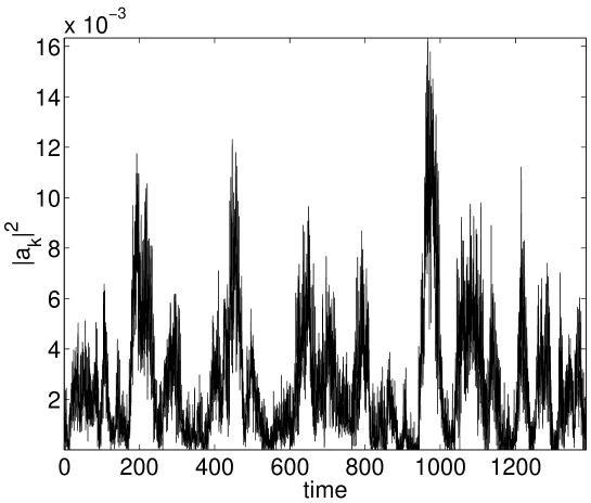
Figure 7: Graph of $A_{k}^{2}(t)$ at wavenumber ${\bf k}=(25,0)$.

Figure 8: Phase evolution, $\phi_{k}(t)$, at wavenumber ${\bf k}=(25,0)$.

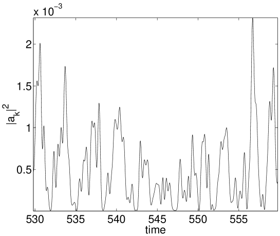
Figure 9: Detailed graph of $A_{k}^{2}(t)$ at wavenumber ${\bf k}=(25,0)$ corresponding to a time interval characterized by low amplitudes and, therefore, phase runs. The linear wave period for this mode is $2\pi/\omega_{k}\approx 1.256$ and the characteristic nonlinear time is of the same order of magnitude.

Figures 7 and 8 show time evolution of the amplitude $A_{k}$ and the (interaction representation) phase $\phi_{k}$ respectively for ${\bf k}=(17,0)$. The phase evolution seen in figure 8 consists of the time intervals when it oscillates quasi-periodically (with amplitude less than $2\pi$) which are inter-leaved by sudden “phase runs”, - fast monotonic phase changes by values which can significantly exceed $2\pi$. By juxtaposing figures 7 and 8, one can see that when the phase runs happen then the amplitude is close to zero. We zoom in at the amplitude graph in a time interval characterized by low amplitudes (and therefore phase runs) in figure 9. One can see large-amplitude quasi-periodic oscillations on $A_{k}$, - it changes in value several-fold over a time comparable to the linear wave period. This indicates that such phase run intervals mark the places where the WT assumption of weak nonlinearity breaks down.

This behavior, together with the two-peak character of the time-Fourier spectrum, suggest that at each wavenumber ${\bf k}$ there are two modes:

$$a_{k}=c_{1}+c_{2}e^{-i\omega^{*}t},$$

where $\omega^{*}>\omega_{k}$ and the complex amplitudes are $c_{1}$ and $c_{2}$ varying in time slower than the linear oscillations. Most of the time $|c_{1}|>|c_{2}|$ and, therefore, the phase $\phi_{k}$ oscillates periodically about the some mean value (equal to the phase of $c_{1}$). However, sometimes $c_{2}$ becomes greater than $c_{1}$ and then the path of $a_{k}$ will encircle zero in the complex plane, so that $\phi_{k}$ starts gaining $2\pi$ for each rotation. These are the phase runs, and in order to trigger these runs the complex-plane path of $a_{k}$ must encircle zero, which explains the observed small values of this quantity during the phase runs. This effect is related to the general phenomenon of phase singularities of complex fields at points of zero amplitude (e.g. [34]). However, our phase runs continue all the time until $c_{2}$ becomes greater than $c_{1}$ and during this time interval (excluding its ends) the amplitude is non-zero and the phase is perfectly regular.

Note that such observed behavior of the phase is very dependent on the wave variables: it occurs in natural variables such as the surface height and velocity but is absent for the waveaction variable after the canonical transformation leading to the Zakharov equation. Thus, the phase runs can say nothing about the dynamics or statistics of the waveaction amplitude used in WT, but they mark short time intervals when nonlinearity fails to be weak for a particular $k$-mode, and this will be used as a diagnostic tool in our simulations.

Figure 10: Phase runs detected in the 2D wavenumber grid over the time period.

In figure 11 we show comparison of the mean rate of the phase change during the upward phase runs and the second peak’s frequency at different wavenumbers. A significant coincidence of these two curves supports the proposed above two-mode explanation.

Figure 11: Mean rate of the phase change during the upward phase runs (thick curve) and the second peak’s frequency (thin curve) as functions of wavenumber.

A word of caution is due about the simple two-mode explanation of the phase runs. Indeed, according to this picture the phase should always run to higher values whereas in figure 8 we see both upward and downward runs. A possible explanation of this is that phase runs may be triggered not only by sharp peaks but also by broadband distributions with frequencies less than the linear one. Such broadband distributions could be made of modes which are strong (and therefore can produce phase runs) but whose duration in time is short and sporadic and at different frequencies (hence a broad spectrum). This picture is supported by the fact that the amount of total wave energy in the frequency range below the linear frequency is similar (and for low wavenumbers even greater) than the amount of energy in the range above the linear frequencies, see figure 13. Evidence of relation of the sub-linear modes and the downward phase runs is shown in figure 12 where the mean rate of the phase change during the downward phase runs and the frequency of the highest sub-linear peak. Again, we can see agreement of these two curves although with a greater level of fluctuations due to the fact the sub-linear modes are very spread over different frequencies.

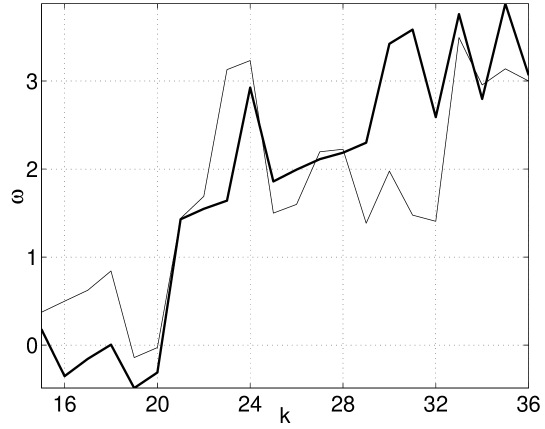
Figure 12: Mean rate of the phase change during the downward phase runs (thick curve) and the frequency of the highest sub-linear peak (thin curve) as functions of wavenumber.

Figure 13: Total energy of modes with frequencies below the linear frequency (solid line) and the modes with frequencies above the linear frequency (dashed line).

7.5 Nonlinearly active modes and cascade “avalanches”

Component with the shifted frequency $\omega^{*}$ is clearly a nonlinear effect (there is no frequency shift in linear dynamics). Thus, the relative strength of $c_{2}$ and $c_{1}$ can be used as a measure of nonlinearity. Particularly, the phase runs mark the events when nonlinearity becomes strong. Figure 10 shows locations of the phase runs in the 2D wavenumber space which happened at $t=500$. Note that at that time ZF steady spectrum has already formed. In the energy cascade range, we see that the phase run density is increasing toward high $k$’s, which is in agreement with the WT prediction that the nonlinearity grows as one cascades down-scale [9, 10]. Curiously, we also observe high density of the phase runs within th circle $k<6$, which is, perhaps, manifestation of a waveaction accumulation via an inverse cascade process. However, this range is too small for any meaningful conclusions to be made about the inverse cascade properties.

The energy cascade from the forcing region toward the high wavenumber region proceeds in a non-uniform in time fashion somewhat resembling sporadic sandpile avalanches. This arises due to the $k$-grid discreteness effects which tend to block the resonant wave interaction when the wave intensities are small. This situation resembles “frozen turbulence” of [14]. Thus, the wave energy does not cascade to high wavenumbers and it tends to accumulate near the forcing scales until the wave intensity is strong enough to restore the resonant interaction via the nonlinear resonance broadening. At this moment the energy cascade toward high wavenumbers sets in, and this leads to depletion of energy at the forcing scale, - “sandpile tips over”. In turn, depletion of energy at the forcing scale leads to blocking of the energy cascade, and the process continues in a repetitive manner. As a result system oscillates between the state of “frozen turbulence” and the state of “avalanche cascade”. This behavior is illustrated in figure 14 which shows percentage of modes experiencing phase runs in two different wavenumber ranges $13<k<29$ and $30<k<45$. One can see that the shapes of these two curves bear a great degree of similarity up to a certain time delay and a vertical shift in the second curve with respect to the first one. The vertical shift reflects the fact that the energy cascade gets stronger as it proceeds to large wavenumbers. The time delay, on the other hand indicates the direction and the character of the sporadic energy cascade. It shows that a higher (lower) nonlinear activity at low $k$’s after a finite delay causes a higher (lower) activity at higher $k$’s, which could be compared with propagation of an avalanche (quenching) down a sandpile.

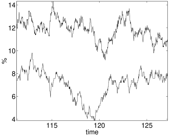
Figure 14: Percentage of modes experiencing phase runs in the range $13<|k|<29$ (lower curve) and in the range $30<|k|<45$ (upper curve).

7.6 Correlations of phases, phase factors and amplitudes.

WT closure relies on the RPA properties of the wave fields, i.e. that the amplitudes $A_{k}$ and the phase factors $\psi_{k}$ are statistically independent variables. On the other hand, WT calculation for the phases $\phi_{k}$ shows that these quantities get correlated. In order to check these properties and predictions numerically, let us introduce a function that measures the degree of statistical dependence (or independence) of some Fourier-space variables $X({\bf k}_{1})$ and $Y({\bf k}_{2})$,

$${\cal C}_{X,Y}({\bf k}_{1},{\bf k}_{2}) = \frac{\langle X({\bf k}_{1})Y({\bf k}_{2})\rangle-\langle X({\bf k}_{1})\rangle\langle Y({\bf k}_{2})\rangle}{\sqrt{\langle X^{2}({\bf k}_{1})\rangle-\langle X({\bf k}_{1})\rangle^{2}}\sqrt{\langle Y^{2}({\bf k}_{2})\rangle-\langle Y({\bf k}_{2})\rangle^{2}}}.$$ (26)

For example, we can examine to what degree amplitudes $A$ and independent of the phase factors $\psi$ by looking at the function ${\cal C}_{A,\psi}({\bf k}_{1},{\bf k}_{2})$ for different values of ${\bf k}_{1}$ and ${\bf k}_{2}$. Independence of the amplitudes at different wavenumbers can be examined by the auto-correlation function ${\cal C}_{A,A}({\bf k}_{1},{\bf k}_{2})$, and similar for the phase factors and the phases. We restrict ourselves with choosing ${\bf k}_{1}=(15,0)$ and ${\bf k}_{2}=(k,0)$ with $k\in(10,64)$. Figure 15 shows the values of correlators ${\cal C}_{\phi,\phi}({\bf k}_{1},{\bf k}_{2})$ and ${\cal C}_{\psi,\psi}({\bf k}_{1},{\bf k}_{2})$ as functions of $k$. In agreement with WT predictions, auto-correlations of $\psi_{k}$’s are very small whereas the ones of $\phi_{k}$’s are significant (except, of course, for $k=15$ where by definition these correlators are equal to one). Correlators ${\cal C}_{A,A}({\bf k}_{1},{\bf k}_{2})$ and ${\cal C}_{A,\psi}({\bf k}_{1},{\bf k}_{2})$ are shown in figure 16. Again, we see a good agreement with the WT prediction: these correlations are very small (except, again, ${\cal C}_{A,A}(15,15)=1$).

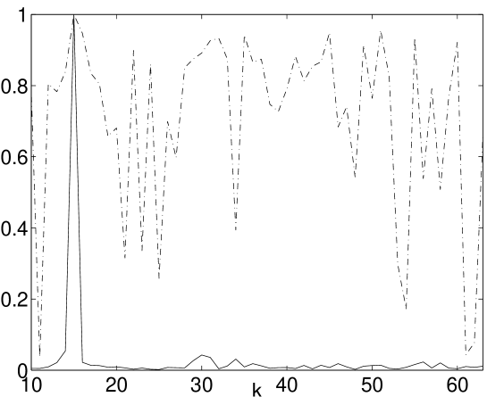
Figure 15: Two-point auto-correlations for the phases ${\cal C}_{\phi,\phi}({\bf k_{1}},{\bf k})$ (dashed line) and for the phase factors ${\cal C}_{\psi,\psi}({\bf k_{1}},{\bf k})$ (solid line) with one point fixed at ${\bf k}=(15,0)$.

Figure 16: Two-point auto-correlation of amplitudes ${\cal C}_{A,A}({\bf k_{1}},{\bf k})$ (thin curve) and two-point correlation between the amplitudes and phase factors ${\cal C}_{A,\psi}({\bf k_{1}},{\bf k})$ (thick curve) with one point fixed at ${\bf k}=(15,0)$.

8 Discussions

In this paper, we used direct numerical simulations of the free water surface in order to examine the statistical properties of the water-wave field beyond the energy spectrum. Our first aim was to check recent predictions of the WT theory about the PDF and intermittency, about the character of correlations of the wave amplitudes and phases. We particularly focused on the question how the effects of discreteness and finite nonlinearity change statistics with respect to the WT closure developed for weak nonlinearities and for a continuous wavenumber space.

Firstly, following [1, 2, 3] we see formation of a quasi-steady spectrum consistent with the Zakharov-Filonenko spectrum predicted by WT. Secondly, we measured PDF for the wave amplitudes and observe an anomalously large, with respect to Gaussian fields, probability of strong waves. This result is in agreement with recent theoretical predictions of [4, 5]. Thirdly, we measure correlations for the amplitudes, phases and phase factors and we observe agreement with predictions of [4, 5]. Namely, the amplitude and the phase correlations behave as statistically independent variables, whereas the phases develop strong auto-correlations over the nonlinear time. Note that these properties are fundamental for the WT closure to work, so in a way we provide a numerical validation for the WT approach.

We also find that at each $k$ there are two sharp frequency peaks: a dominant one at the linear frequency and a weaker one with a frequency shift arising due to the $k/2$-mode. Somewhat related to this two-peak frequency structure is the observed time behavior of the phase. We observe calm periods during which the phase oscillates within $2\pi$-wide margins intermittent with sudden phase runs during which it experiences a monotonic change significantly greater than $2\pi$.

Finally, we observe that the energy cascade is “bursty” in time and is somewhat similar to sporadic sandpile avalanches. We give a plausible explanation of this behavior as an interplay of effects of discreteness and nonlinearity. Because in between of the avalanche discharges the resonances are absent then, at least qualitatively, one can refer to the KAM theory and say that the evolution should remain close to the corresponding integrable case, - the linear system in our case. This picture is supported by a simple analysis of quasi-resonances given in this paper which indicates that there exists a single threshold value of turbulence intensity at the forcing scale separating the no-cascade and unlimited (in $k$) cascade regimes.

A further numerical study of the avalanche effect is desirable, particularly using a different wavenumber grid and using a more direct method of measuring the turbulent flux and its correlations for different inertial interval points.

9 Acknowledgments

We thank Miguel Onorato and Victor Shrira for helping us to understand the nature of the second frequency peak, and Miles Reid for teaching us some Number Theory basics.

References

- [1] A.I. Dyachenko, A.O. Korotkevich, V.E. Zakharov, Weak turbulence of gravity waves, JETP Letters, 77, No. 10, 2003; Phys. Rev. Lett., 92, 13, 134501 (2004).
- [2] M. Onorato et.al., Freely decaying weak turbulence for sea surface gravity waves, Phys.Review L 89 No.14, September 2002.
- [3] N. Yokoyama, Statistics of Gravity Waves obtained by direct numerical simulation, JFM 501, 169-178 (2004).
- [4] Y. Choi, Y.V. Lvov, S. Nazarenko,B. Pokorni, Anomalous probability of large amplitudes in wave turbulence, Physics Letters A, 339, Issue 3-5, p. 361-369 (also on arXiv:math-ph/0404022 v1 & Apr 2004).
- [5] Y. Choi, Y.V. Lvov, S. Nazarenko, Probability Densities and Preservation of Randomness in Wave Turbulence Physics Letters A, 332, 230-238 (2004); Joint statistics of amplitudes and phases in wave turbulence, Physica D 201 (2005) 121-149; Y.Choi, Y.V. Lvov, S. Nazarenko; Wave turbulence, in ”Recent developments in fluid dynamics” 5 (2004), Transworld Research Network, Kepala, India (also on arXiv.org:math-ph/0412045).
- [6] Y. Lvov and S. Nazarenko, ”Noisy” spectra, long correlations and intermittency in wave turbulence, Phys. Rev. E 69, 066608 (2004)
- [7] K. Hasselmann, J. Fluid Mech 12 481 (1962).
- [8] V.E.Zakharov and Filonenko, J. Appl. Mech. Tech. Phys. 4 506-515 (1967).
- [9] A.C. Newell, V.E. Zakharov, Rough sea foam, PRL 69 No.8, August 1992.
- [10] L. Biven, S.V. Nazarenko and A.C. Newell, ”Breakdown of wave turbulence and the onset of intermittency” Phys Lett A, 280, 28-32, (2001). A.C. Newell, S.V. Nazarenko and L. Biven, Physica D, 152-153, 520-550, (2001).
- [11] S. Nazarenko, “Sandpile behaviour in discrete water-wave turbulence”, J. Stat. Mech. (2006) L02002 doi:10.1088/1742-5468/2006/02/L02002 (arXiv: nlin.CD/0510054).
- [12] Peter A.E.M. Janssen, Nonlinear four-wave interactions and freak waves, Journal of Phys.Oceanography, 33, April 2003.
- [13] V.I. Shrira, D.V. Ivonin, P. Broche and J.C. Maistre, On remote sensing of vertical sheer of ocean surface currents by means of a single-frequency VHF radar, Geophys. Res. Lett, 28, p 3955 (2001).
- [14] A.N. Pushkarev, On the Kolmogorov and frozen turbulence in numerical simulation of capillary waves, Eur. J. Mech. B/Fluids 18, 345-352 (1999)
- [15] Choi, W. Nonlinear evolution equations for two-dimensional surface waves in a fluid of finite depth. J. Fluid Mech. 295, 381-394, (1995).
- [16] V.E. Zakharov, V.S. L’vov and G.Falkovich, ”Kolmogorov Spectra of Turbulence”, Springer-Verlag, 1992.
- [17] V.E. Zakharov, Stability of periodic waves of finite amplitude on surface of deep water, PMFT, No 2 (1968) 86-94.
- [18] V.E. Zakharov, Inverse and direct cascade in the wind-driven surface wave turbulence and wave-breaking, Proceedings of IUTAM Meeting on Wave Breaking (Sydney, 1991).
- [19] V.E. Zakharov, Weakly nonlinear waves on the surface of an ideal fluid, AMS Transl. 182, 1998.
- [20] A.N. Pushkarev, D. Resio, V.E. Zakharov, Weak turbulent approach to the wind-generated gravity sea waves, Physica D 184 (1-4) 29-63 (2003).
- [21] V. P. Krasitskii, On reduced equations in the Hamiltonian theory of weakly nonlinear surface-waves, J. Fluid Mech. 272, (1994) 1.
- [22] B. Rumpf and L. Biven, Weak turbulence and collapses in the Majda-Mc-Laughlin-Tabak equation: Fluxes in wavenumber and in amplitude space. Physica D 204 (2005), 188-203 (also on oai:arXiv.org:nlin/0503005 ).
- [23] E.A. Kartashova, On properties of weakly nonlinear wave interactions in resonators Physica D 54 (1-2): 125-134 Dec 1991; E.A. Kartashova, Weakly nonlinear theory of finite-size effects in resonators Phys.Rev.Lett 72 (13) 2013-2016, Mar 28, 1994; E. Kartashova, Wave resonances in systems with discrete spectra, AMS Transl. (2) 182, 1998.
- [24] A.I. Dyachenko, Y.V. Lvov, V.E. Zakharov, Five-wave interaction on the surface of deep fluid, Physica D 87 (1-4) 233-261 (1995).
- [25] Kartashova, Private Communications, 2006.
- [26] O. M. Phillips, On the dynamics of unsteady gravity waves of finite amplitude. 1. The elementary interactions J. Fluid Mech. 9 (1960) 193.
- [27] A.I. Dyachenko and V.E. Zakharov, Is free surface hydrodynamics an integrable system?, Physics Letters A 190 (2) (1994) 144-148.
- [28] C.Connaughton, S.Nazarenko, A. Pushkarev, Discreteness and quasiresonances in weak turbulence of capillary waves, Physical Review E, 63, 046306, (2001).
- [29] M.Tanaka, N.Yokoyama, Effects of discretization of the spectrum in water-wave turbulence, Fluid Dynamics Research 34 (2004) 199-216.
- [30] V.E. Zakharov, A.O. Korotkevich, A.N. Pushkarev and A.I. Dyachenko, Mesoscopic wave turbulence, 82, 8, 487-491 (2005).
- [31] S.N. Papakostas, Ch. Tsitouras, High phase-lag-order Runge-Kutta and Nystrom pairs, SIAM J.Sci.Comput. 21 No2, 1999.
- [32] V.E.Zakharov Statistical theory of gravity and capillar y waves on the surface of a finite-depth fluid, Eur.J.Mech. B/Fluids, 1999.
- [33] A.I.Dyachenko, Y.V.Lvov On the Hasselmann and Zakharov approaches to the kinetic equation for gravity waves, J.Phys.Oceanography, 2 5, No.12, December 1995.
- [34] M.V. Berry and M.R. Dennis, Phase singularities in isotropic random waves, Proc. Roy. Soc A 456 2059-2079 (2000).