Relations between Potts and RSOS models on a torus

Abstract

We study the relationship between $Q$-state Potts models and staggered RSOS models of the $A_{p-1}$ type on a torus, with $Q^{1/2}=2\cos(\pi/p)$. In general the partition functions of these models differ due to clusters of non-trivial topology. However we find exact identities, valid for any temperature and any finite size of the torus, between various modified partition functions in the two pictures. The field theoretic interpretation of these modified partition function is discussed.

I Introduction

The two-dimensional Potts model Wu82 ; Saleur91 can be defined in terms of integer valued spins $S_{i}=1,2,\ldots,Q$ living on the vertices $\{i\}$ of a lattice. Its partition function reads

$$Z_{\rm spin}=\sum_{\{S_{i}\}}\prod_{\langle ij\rangle}{\rm e}^{K\delta(S_{i},S_{j})},$$ (1)

where $\delta$ is the Kronecker delta and $\langle ij\rangle$ are the lattice edges. In this paper we take the lattice to be an $L\times N$ square lattice (say, of vertical width $L$ and horizontal length $N$) with toroidal boundary conditions (i.e., periodic boundary conditions in both lattice directions). We denote $V=LN$ the number of vertices of the lattice and $E=2LN$ the number of edges.

This initial definition can be extended to arbitrary real values of $Q$ by means of a cluster expansion Kasteleyn . One finds

$$Z_{\rm cluster}=\sum_{\cal C}v^{e({\cal C})}Q^{c({\cal C})},$$ (2)

where $v={\rm e}^{K}-1$. Here, the sum is over the $2^{E}$ possible colourings ${\cal C}$ of the lattice edges (each edge being either coloured or uncoloured), $e({\cal C})$ is the number of coloured edges, and $c({\cal C})$ is the number of connected components (clusters) formed by the coloured edges. For $Q$ a positive integer one has $Z_{\rm spin}=Z_{\rm cluster}$.

Yet another formulation is possible when $Q^{1/2}=q+q^{-1}$ and $q$ is a root of unity

$$q={\rm e}^{i\pi/p},\qquad p=3,4,5,\ldots,$$ (3)

this time in terms of a restricted height model with face interactions ABF ; Pasquier ; PS , henceforth referred to as the RSOS model. This formulation is most easily described in an algebraic way. The Potts model transfer matrix $T$ that adds one column of the square lattice can be written in terms of the generators $e_{j}$ of the Temperley-Lieb algebra TL as follows

$$T = Q^{L/2}H_{L}\cdots H_{2}H_{1}V_{L}\cdots V_{2}V_{1},$$ (4)

$$H_{i} = xI_{2i-1}+e_{2i-1},$$

$$V_{i} = I_{2i}+xe_{2i}.$$

Here, $H_{i}$ and $V_{i}$ are operators adding respectively horizontal and vertical edges to the lattice, $I_{j}$ is the identity operator acting at site $j$, and the parameter $x=Q^{-1/2}v=Q^{-1/2}({\rm e}^{K}-1)$. The generators satisfy the well-known algebraic relations

$$e_{i}e_{i\pm 1}e_{i} = e_{i},$$

$$(e_{i})^{2} = Q^{1/2}e_{i},$$ (5)

$$e_{i}e_{j} = e_{j}e_{i}\mbox{ for $|i-j|\geq 2$}.$$ (6)

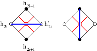
Figure 1: Graphical rendering of $V_{i}=I_{2i}+xe_{2i}$. Direct (resp. dual) vertices are shown as full (resp. empty) circles. Coloured edges (direct and dual) in the cluster picture are depicted as thick blue lines. Their surrounding cluster boundaries are given as thin red lines. RSOS heights $h_{j}$ are defined on both direct and dual vertices as shown. The action of $I_{2i}$ (resp. $e_{2i}$) is illustrated on the left (resp. right) part of the figure. Our convention is that the transfer matrix acts towards the right.

More precisely, $V_{i}$ can be thought of as adding a face to the lattice, surrounded by two direct and two dual vertices, as shown in Fig. 1. $H_{i}$ is similarly defined, by exchanging direct and dual sites on the figure.

Meanwhile, the operators $I_{j}$ and $e_{j}$ can be represented in various ways, thus giving rise to different transfer matrices. When $Q$ is a positive integer, a spin representation of dimension $Q^{L}$ can be defined in an obvious way, and one has

$$Z_{\rm spin}={\rm Tr}\ (T_{\rm spin})^{N}.$$ (7)

For any real $Q$ a cluster representation Blote82 of dimension $C_{L}=\frac{(2L)!}{(L+1)!\,L!}$ can be defined by letting $I_{j}$ and $e_{j}$ act on the boundaries BKW ; BaxterBook that separate direct and dual clusters, represented as thin red lines in Fig. 1. But it is impossible to write $Z_{\rm cluster}$ as a trace of $T_{\rm cluster}$ defined in this way. This is due to the existence of loops of cluster boundaries that are non contractible with respect to the periodic boundary conditions in the horizontal direction of the lattice. For this reason, we shall not discuss $T_{\rm cluster}$ much further in this paper, but we maintain Eq. (2) as the definition of $Z_{\rm cluster}$ for real $Q$.

Finally, when $Q$ is given by Eq. (3) the RSOS model is introduced by letting $I_{j}$ and $e_{j}$ act on heights $h_{j}=1,2,\ldots,p-1$ defined on direct and dual vertices ABF ; Pasquier . A pair of neighbouring direct and dual heights are constrained to differ by $\pm 1$. In this representation we have

$$I_{j}=\delta(h_{j},h^{\prime}_{j}),\qquad e_{j}=\delta(h_{j-1},h_{j+1})\left(S_{h_{j}}S_{h^{\prime}_{j}}\right)^{1/2}\left(S_{h_{j-1}}\right)^{-1},$$ (8)

where $S_{h}=\sin(\pi h/p)$. Note that the clusters (direct and dual) are still meaningful as they are surfaces of constant height. The constants $S_{h}$ are actually the components of the Perron-Frobenius eigenvector of the incidence matrix (of size $p-1$)

$$G_{p-1}=\left(\begin{tabular}[]{ccccc}0&1&0&$\cdots$&0\vspace{-0.2cm}\\ 1&0&1&&$\vdots$\vspace{-0.2cm}\\ 0&$\ddots$&$\ddots$&$\ddots$&0\vspace{-0.2cm}\\ $\vdots$&&1&0&1\vspace{0.05cm}\\ 0&$\cdots$&0&1&0\\ \end{tabular}\right)$$ (9)

of the Dynkin diagram $A_{p-1}$ Pasquier . In this representation, of dimension ${\rm Tr}\,(G_{p-1})^{2L}\sim Q^{L}$, we now define the transfer matrix $T_{\rm RSOS}$ by Eq. (4) and the partition function $Z_{\rm RSOS}={\rm Tr}\,(T_{\rm RSOS})^{N}$, the trace being over allowed height configurations.

In this paper we discuss the relations between $Z_{\rm RSOS}$ and $Z_{\rm cluster}$, with $Q^{1/2}=2\cos(\pi/p)$ cf. Eq. (3). These partition functions are in general different, due to clusters of non-trivial topology wrapping around the torus.

We start by showing numerically, in section II, that for $Q=3$ the transfer matrices $T_{\rm spin}$ and $T_{\rm RSOS}$ have nonetheless many identical eigenvalues. Defining various sectors (motivated by duality and parity considerations) and also twisting the periodic boundary conditions in different ways, we are able to conjecture several relations between the corresponding transfer matrix spectra.

With this numerical motivation we then go on, in section III, to prove these relations on the level of the RSOS and cluster model partition functions on finite $L\times N$ tori. Some of the relations are specific to $Q=2$ ($p=4$) and $Q=3$ ($p=6$), and some hold for general values of $p$. All of them hold for arbitrary values of the temperature variable $x$. We stress that in all cases the proofs are based on rigorous combinatorial considerations.

We conclude the paper, in section IV, by interpreting our results, and the various partition functions introduced, on the level of conformal field theory, at the selfdual temperature $x=1$ where the Potts model is at a critical point.

II Transfer matrix spectra

The spectra of the transfer matrices $T_{\rm spin}$ and $T_{\rm RSOS}$ are easily studied numerically by exact diagonalisation techniques. Denoting the eigenvalues as $\Lambda_{i}$, with $i=1,2,\ldots,{\rm dim}(T)$, the results are most conveniently stated in terms of the corresponding free energies per spin, $f_{i}=-L^{-1}\log(\Lambda_{i})$. Sample results for $Q=3$, width $L=2$, and temperature variable $x=5$ are shown in Table 1.

Transfer matrix:	$T_{\rm RSOS}^{\rm even}$	$T_{\rm RSOS}^{\rm odd}$	$T_{\rm spin}$	$T_{\rm spin}^{\rm dual}$
Twist:	$I$  $Z_{2}$	$I$  $Z_{2}$	$I$  $Z_{2}$  $Z_{3}$	$I$  $Z_{2}$  $Z_{3}$
-4.547135105405	1   0	1   0	1    0    0	1    0    0
-4.536300662409	1   0	1   0	0    1    0	0    1    0
-4.530748290953	1   1	0   0	2    0    0	0    0    1
-3.512711596812	0   0	1   1	0    0    1	2    0    0
-3.502223380184	1   0	1   0	0    1    0	0    1    0
-3.441474985184	0   0	0   0	0    0    2	0    0    2
-3.397645107750	0   2	0   2	0    2    0	0    2    0
-3.348639214318	0   0	0   0	0    0    2	0    0    2
-3.292754029664	1   0	2   1	0    1    1	2    1    0
-2.335814864962	1   0	1   0	1    0    0	1    0    0
-2.307465012288	2   1	1   0	2    1    0	0    1    1
-2.285900912958	1   0	1   0	0    1    0	0    1    0
-2.251579827634	0   0	0   0	0    0    2	0    0    2
-2.236228400659	0   0	1   1	0    0    1	2    0    0
-2.203480723895	1   1	0   0	2    0    0	0    0    1
-2.202573934202	0   2	0   2	0    2    0	0    2    0
-2.158744056768	0   1	0   1	1    0    0	1    0    0

Table 1: Spectra of various transfer matrices with $Q=3$, subject to periodic ($I$) or different twisted periodic ($Z_{2}$ and $Z_{3}$) boundary conditions, as defined in the text. The first column gives the free energies $f_{i}=-L^{-1}\log(\Lambda_{i})$, here for width $L=2$ and temperature variable $x=5$. Subsequent columns give the multiplicity of each $f_{i}$.

Due to the rules of the RSOS model, the heights living on the direct and dual lattices have opposite parities. The transfer matrix can therefore be decomposed in two sectors, $T_{\rm RSOS}=T_{\rm RSOS}^{\rm even}\oplus T_{\rm RSOS}^{\rm odd}$, henceforth referred to as even and odd. In the even sector, direct heights take odd values and dual heights even values (and vice versa for the odd sector). Results with standard (i.e., untwisted) periodic boundary conditions in the vertical direction are given in the columns labeled $I$ in Table 1.

In the spin representation $T_{\rm spin}(x)$ has been defined above (recall that $x=Q^{-1/2}({\rm e}^{K}-1)$). We also introduce a related transfer matrix

$$T_{\rm spin}^{\rm dual}(x)\equiv x^{2L}T_{\rm spin}(x^{-1}),$$ (10)

as well as the corresponding partition function $Z_{\rm spin}^{\rm dual}(x)\equiv{\rm Tr}\,(T_{\rm spin}^{\rm dual}(x))^{N}$. The appearance of the dual temperature, $x_{\rm dual}=x^{-1}$ explains the terminology. More precisely, on a planar lattice one has the fundamental duality relation Wu82

$$Z_{\rm spin}(x)=Q^{-1}x^{E}\tilde{Z}_{\rm spin}(x^{-1}),$$ (11)

where $\tilde{Z}$ must be evaluated on the dual lattice. For a square lattice with toroidal boundary conditions, the dual and direct lattices are isomorphic, but Eq. (11) breaks down because of effects of non-planarity.

Referring to Table 1, we observe that the leading eigenvalues of the four transfer matrices introduced this far (i.e., $T_{\rm RSOS}^{\rm even}$, $T_{\rm RSOS}^{\rm odd}$, $T_{\rm spin}$ and $T_{\rm spin}^{\rm dual}$) all coincide. On the other hand, for any two $T$ chosen among these four, some of the sub-leading eigenvalues coincide, whilst others are different. So the discrepancy between the four corresponding partition functions appears to be a boundary effect which vanishes in limit $N\to\infty$. However, when taking differences of the multiplicities we discover a surprising relation:

$$2(Z^{\rm even}_{\rm RSOS}(x)-Z^{\rm odd}_{\rm RSOS}(x))=Z_{\rm spin}(x)-Z^{\rm dual}_{\rm spin}(x).$$ (12)

Note that the leading eigenvalues cancel on both sides of this relation.

At the selfdual point $x=1$, we find that the spectra of $T_{\rm RSOS}^{\rm even}$ and $T_{\rm RSOS}^{\rm odd}$ coincide completely, as do those of $T_{\rm spin}$ and $T_{\rm spin}^{\rm dual}$. In particular, both sides of Eq. (12) vanish. It is however still true that subleading eigenvalues of $T_{\rm RSOS}^{\rm even}$ and $T_{\rm spin}$ differ.

More relations can be discovered by introducing twisted periodic boundary conditions in the transfer matrices. For the RSOS model this can be done by twisting the heights, $h\to p-h$, when traversing a horizontal seam. Note that this transformation makes sense at it leaves the weights of Eq. (8) invariant, since $S_{h}=S_{p-h}$. The shape of the seam can be deformed locally without changing the corresponding partition function; we can thus state more correctly that the seam must be homotopic to the horizontal principal cycle of the torus. Note also that the twist is only well defined for even $p$ (and in particular for $Q=3$, $p=6$), since the heights on the direct and dual lattice must have fixed and opposite parities in order to satisfy the RSOS constraint. In Table 1, this twist is labeled $Z_{2}$, since it amounts to exploiting the $Z_{2}$ symmetry of the underlying Dynkin diagram $A_{p-1}$. Comparing again multiplicities we discover a second relation

$$Z^{\rm even}_{\rm RSOS}(x)-Z^{\rm odd}_{\rm RSOS}(x)=Z^{{\rm even},Z_{2}}_{\rm RSOS}(x)-Z^{{\rm odd},Z_{2}}_{\rm RSOS}(x).$$ (13)

The relations (12) and (13) are special cases of relations that hold for all $x$, $L$ and $N$, and for all even $p$. The general relations (see Eqs. (30) and (37)) are stated and proved in section III below.

In the particular case of $Q=3$ one can define two different ways of twisting the spin representation, which will lead to further relations. The first type of twist shall be referred to as a $Z_{2}$ twist, and consist in interchanging spin states $S_{i}=1$ and $S_{i}=2$ across a horizontal seam, whereas the spin state $S_{i}=3$ transforms trivially. The second type of twist, the $Z_{3}$ twist, consists in permuting the three spin states cyclically when traversing a horizontal seam. The spectra of the corresponding transfer matrices are given in Table 1.

This leads to another relation between the spectra in the spin representation (stated here in terms of the corresponding partition functions)

$$Z^{Z_{2}}_{\rm spin}(x)=Z^{{\rm dual},Z_{2}}_{\rm spin}(x),$$ (14)

as well a two further relations linking the spin and RSOS representations:

$$Z^{\rm even}_{\rm RSOS}(x)-Z^{\rm odd}_{\rm RSOS}(x) = -\left(Z^{Z_{3}}_{\rm spin}(x)-Z^{{\rm dual},Z_{3}}_{\rm spin}(x)\right),$$ (15)

$$Z^{\rm even}_{\rm RSOS}(x)+Z^{{\rm even},Z_{2}}_{\rm RSOS}(x) = Z_{\rm spin}(x)+Z^{Z_{2}}_{\rm spin}(x).$$ (16)

These relations are proved in section III.10 below.

III Relations between partition functions

III.1 Weights in the cluster and RSOS pictures

A possible configuration of clusters on a $6\times 6$ torus is shown in Fig. 2. It can be thought of as a random tessellation using the two tiles of Fig. 1. For simplicity we show here only the clusters (direct or dual) and not their separating boundaries (given by the thin red lines in Fig. 1). Two clusters having a common boundary are said to be neighbouring. For convenience in visualising the periodic boundary conditions the thick lines depicting the clusters have been drawn using different colours (apart from clusters consisting of just one isolated vertex, which are all black).

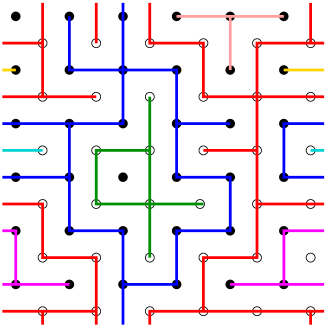
Figure 2: A possible cluster configuration on a $6\times 6$ torus. Direct and dual vertices are shown as filled and empty black circles. Clusters (direct or dual), other than isolated vertices, are depicted here using distinct colours, for convenience in appreciating the periodic boundary conditions. There are six direct clusters and four dual clusters. One direct cluster and one dual cluster are non-homotopic to a point.

To compute the contribution of this configuration to $Z_{\rm cluster}(x)$, each direct cluster is weighed by a factor of $Q$, and each coloured direct edge carries a factor of $v=Q^{1/2}x$. Note in particular that the cluster representation does not distinguish clusters of non-trivial topology (i.e., clusters which are not homotopic to a point). In the following we shall call such clusters non-trivial; clusters which are homotopic to a point are then referred to as trivial.

The contribution of this same configuration to $Z_{\rm RSOS}$ consists of

1. a global factor of $Q^{V/2}$ coming from the prefactor of Eq. (4),

2. a factor of $x$ for each coloured direct edge SB , and

3. an $x$-independent factor due to the topology of the (direct and dual) clusters Pasquier .

The interest is clearly concentrated on this latter, topological factor which we denote $w$ in the following. For a given cluster configuration its value can be computed from the adjacency information of the clusters. This information is conveniently expressed in the form of a Pasquier graph Pasquier ; for the cluster configuration of Fig. 2 this graph is shown in Fig. 3.

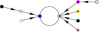
Figure 3: Pasquier graph corresponding to the cluster configuration of Fig. 2. Direct (resp. dual) clusters are shown as filled (resp. empty) circles, using the same colour coding as in Fig. 2. Neighbouring clusters are connected by an edge. The arrows are explained in the text.

The rules for drawing the Pasquier graph in the general case are as follows. Each cluster is represented by a vertex, and vertices representing neighbouring clusters (i.e., clusters having a common boundary) are joined by a directed edge. An edge directed from vertex $A$ to vertex $B$ means that the common boundary is surrounding cluster $A$ and is surrounded by cluster $B$. In particular, the in-degree $b_{\rm in}$ of a cluster is the number of boundaries surrounded by that cluster, and the out-degree $b_{\rm out}$ is the number of boundaries surrounding the cluster. By definition, a boundary separating a non-trivial cluster from a trivial one is said to be surrounded by the non-trivial cluster; note that there is necessarily at least one non-trivial cluster. We do not assign any orientation to edges joining two non-trivial clusters, since in that case the notion of surrounding is nonsensical.

The topological structure of the Pasquier graph is characterised by the following three properties:

1. The graph is bicolourable, with one colour (represented by filled circles in Fig. 3) corresponding to direct clusters and the other (empty circles in Fig. 3) to dual clusters.

2. The vertices corresponding to non-trivial clusters and the undirected edges form a cycle.

3. Each vertex corresponding to a non-trivial cluster is the root of a (possible empty) tree, whose vertices correspond to trivial clusters. The edges in the tree are directed towards the root.

Property 3 is easily proved by noticing that vertices corresponding to trivial clusters have all $b_{\rm out}=1$, i.e., such clusters have a unique external boundary. Regarding property 2, we shall define the order $n$ of the Pasquier graph as the number of undirected edges. By property 1, $n$ is even. When $n=0$ we shall call the graph degenerate; this corresponds to a situation in which a single cluster (direct or dual) is non-trivial.

In the RSOS picture, each configuration of the clusters (such as the one on Fig. 2) corresponds to many different height configurations. The topological ($x$-independent) contribution to the weight of a cluster configuration in $Z_{\rm RSOS}$ is therefore obtained by summing weights in the RSOS model with $x=1$ over all height configurations which are compatible with the given cluster configuration Pasquier . This contribution can be computed from the Pasquier graph by using the incidence matrix $G_{p-1}$ of the Dynkin diagram $A_{p-1}$, as we now review.

Let $w$ be the weight of a given Pasquier graph, and let $w^{\prime}$ be the weight of the graph in which a leaf of one of its trees (as well as its adjacent outgoing edge) has been removed. More precisely, $w$ is the weight of a cluster configuration with given heights on each cluster, and $w^{\prime}$ is the partial sum of such weights over all possible heights of the leaf cluster. Let $j$ be the height of the leaf, and let $i$ be the height of its parent. Then

$$w=w^{\prime}(S_{i})^{-1}\sum_{1\leq j\leq p-1}(G_{p-1})_{ij}S_{j}=w^{\prime}(S_{i})^{-1}Q^{1/2}S_{i}=Q^{1/2}w^{\prime},$$ (17)

where in the first equality we used that the weight of a cluster at height $h$ is $S_{h}^{b_{\rm out}-b_{\rm in}}$ Pasquier , and in the second that $\{S_{j}\}$ is an eigenvector of $G_{p-1}$ with eigenvalue $Q^{1/2}$. Iterating the argument until all the trees of the Pasquier graph have been removed, we conclude that each trivial cluster carries the weight $Q^{1/2}$.

We have then

$$w=Q^{(l-n)/2}w_{\rm c},$$ (18)

where $w_{\rm c}$ is the weight of the cycle of the Pasquier graph. It corresponds to the number of closed paths of length $n$ on the Dynkin diagram

$$w_{\rm c}={\rm Tr}\,(G_{p-1})^{n}=\sum_{1\leq k\leq p-1}\left(2\cos(k\pi/p)\right)^{n},$$ (19)

where we have used the eigenvalues of $G_{p-1}$. Note that, in contrast to the case of trivial clusters, all the eigenvalues contribute to the combined weight $w_{\rm c}$ of the non-trivial clusters, and that this weight cannot in general be interpreted as a product of individual cluster weights. (We also remark that it is not a priori obvious that the right-hand side of Eq. (19) is an integer.)

III.2 Coincidence of highest eigenvalues

As an application we now argue that the dominant eigenvalues of the transfer matrices $T_{\rm RSOS}$, $T_{\rm cluster}$, $T_{\rm spin}$ coincide for any width $L$. We suppose $x>0$ so that all weights are positive; this guarantees in particular that standard probabilistic arguments apply.

Consider first $T_{\rm cluster}$ and $T_{\rm spin}$, supposing $Q$ a positive integer. Since the system is quasi one-dimensional, with $L\ll N$, configurations having clusters of linear extent much larger than $L$ are exceedingly rare and can be neglected. In particular, almost surely no cluster will wrap around the system in the horizontal direction. Writing $Z_{\rm cluster}\sim(\Lambda_{\rm c})^{N}$ and $Z_{\rm spin}\sim(\Lambda_{\rm s})^{N}$, the choice of boundary conditions in the horizontal direction will thus have no effect on the values of $\Lambda_{\rm c}$ and $\Lambda_{\rm s}$. We therefore switch to free boundary conditions in the horizontal direction. Then it is possible Salas01 to write $Z_{\rm cluster}=\langle f|(T_{\rm cluster})^{N}|i\rangle$ for suitable initial and final vectors $|i\rangle$ and $\langle f|$. It is not difficult to see, using the Perron-Frobenius theorem, that these vectors both contain a non-vanishing component of the dominant eigenvector of $T_{\rm cluster}$. We conclude that $\Lambda_{\rm c}$ must be the dominant eigenvalue of $T_{\rm cluster}$. Likewise, $\Lambda_{\rm s}$ is the dominant eigenvalue of $T_{\rm spin}$. The conclusion follows by noting that $Z_{\rm cluster}=Z_{\rm spin}$ by construction.

We now turn to $T_{\rm RSOS}$ and $T_{\rm cluster}$, supposing $Q^{1/2}=2\cos(\pi/p)$, cf. Eq. (3). As before we impose free horizontal boundary conditions on the cluster model. Then, since the resulting lattice is planar, we recall that $Z_{\rm cluster}$ can be written as well in terms of the boundaries separating direct and dual clusters BKW ; BaxterBook

$$Z_{\rm cluster}=Q^{V/2}\sum_{\cal C}x^{e({\cal C})}Q^{l({\cal C})/2},$$ (20)

where the configurations ${\cal C}$ correspond bijectively to those of Eq. (2), and $l({\cal C})$ is the number of cluster boundaries (loops). For $N\to\infty$ we have $Z_{\rm RSOS}\sim(\Lambda_{\rm r})^{N}$, and to conclude that $\Lambda_{\rm r}=\Lambda_{\rm c}$ it suffices to show that asymptotically $Z_{\rm RSOS}\sim Z_{\rm cluster}$. Consider now a typical cluster configuration. Almost surely, the corresponding Pasquier diagram will be of order $n\sim N$, and in particular $n\gg 1$. Hence $w_{\rm c}\sim Q^{n/2}$ from Eq. (19). It follows that also in the RSOS picture each cluster boundary carries the weight $Q^{1/2}$, regardless of its homotopy. The conclusion follows.

In section II we have introduced the decomposition of the RSOS model into even and odd subsectors. In the even sector, heights on direct (resp. dual) clusters are odd (resp. even). In particular, we have $Z_{\rm RSOS}=Z_{\rm RSOS}^{\rm even}+Z_{\rm RSOS}^{\rm odd}$. Note that since that the largest and smallest eigenvalue in Eq. (19) differ just by a sign change, we have the slightly more precise statement for $N\to\infty$:

$$Z_{\rm RSOS}\simeq 2Z_{\rm RSOS}^{\rm even}\simeq 2Z_{\rm RSOS}^{\rm odd}\simeq 2Z_{\rm cluster}.$$ (21)

In particular, the largest eigenvalues of $T_{\rm RSOS}^{\rm even}$ and $T_{\rm RSOS}^{\rm odd}$ coincide, in agreement with the numerical data of Table 1.

III.3 Duality relation for $Z_{\rm RSOS}^{\rm even}-Z_{\rm RSOS}^{\rm odd}$

We now compare the contributions to the partition functions $Z_{\rm RSOS}^{\rm even}$ and $Z_{\rm RSOS}^{\rm odd}$ for a given cluster configuration (summed over all possible heights assignments with the specified parity). The argument that trivial clusters carry a weight $Q^{1/2}$ is unchanged, cf. Eq. (17), and holds irrespective of parity. We can thus limit the discussion to the weight $w_{\rm c}$ of the cycle in the Pasquier graph.

We first show that

$$w_{\rm c}^{\rm even}=w_{\rm c}^{\rm odd}=\frac{1}{2}{\rm Tr}\,(G_{p-1})^{n}$$ (22)

for non-degenerate Pasquier graphs (i.e., of order $n\neq 0$). In this non-degenerate case, the numbers of direct and dual non-trivial clusters are equal, whence $n=2k$ is even. By definition $w_{\rm c}^{\rm even}$ is the number of height assignments $\{h_{1},h_{2},\ldots,h_{2k}\}$ such that $h_{i}=1,2,\ldots,p-1$ and $|h_{i+1}-h_{i}|=1$ (we consider $i$ modulo $2k$), with $h_{1}$ even. Now by a cyclic relabeling, $i\to i+1$ (mod $2k$), each such height assignment is mapped bijectively to a height assignment in which $h_{1}$ is odd. It follows that $w_{\rm c}^{\rm even}=w_{\rm c}^{\rm odd}$.

Consider now the degenerate case $n=0$ with just a single non-trivial cluster (which will then span both periodic directions of the torus). Then, counting just the number of available heights of a given parity, the contribution of the cycle to respectively $Z_{\rm RSOS}^{\rm even}$ and $Z_{\rm RSOS}^{\rm odd}$ read ($\lfloor x\rfloor$ denotes the integer part of $x$)

$$w_{\rm c}^{\rm even}=\lfloor p/2\rfloor,\qquad w_{\rm c}^{\rm odd}=\lfloor(p-1)/2\rfloor,$$ (23)

if the non-trivial cluster is direct (if it is dual, permute the labels even and odd). In particular, $w_{\rm c}^{\rm even}=w_{\rm c}^{\rm odd}$ for $p$ odd and we deduce that

$$Z_{\rm RSOS}^{\rm even}(x)=Z_{\rm RSOS}^{\rm odd}(x)\mbox{ for $p$ odd}.$$ (24)

Of course, Eq. (24) can be proved in a much more elementary way by noticing that for $p$ odd the RSOS model is symmetric under the transformation $h\to p-h$, which exchanges the parity of the heights. This even implies the stronger statement $T_{\rm RSOS}^{\rm even}=T_{\rm RSOS}^{\rm odd}$. On the other hand, for $p$ even, the transformation $h\to p-h$ does not change the parity, and $T_{\rm RSOS}^{\rm even}\neq T_{\rm RSOS}^{\rm odd}$; the two matrices do not even have the same dimension.

The purpose of presenting the longer argument leading to Eq. (24) is to make manifest that this relation breaks down for even $p$ exactly because of configurations represented by degenerate Pasquier graphs. However a weaker relation holds true for any parity of $p$:

$$Z_{\rm RSOS}^{\rm even}(x)=x^{E}Z_{\rm RSOS}^{\rm odd}(x^{-1}).$$ (25)

Note that it implies, as a corollary, that Eq. (24) also holds for $p$ even provided that $x=1$.

To prove Eq. (25) we again argue configuration by configuration. Each cluster configuration is in bijection with a “shifted” configuration obtained by keeping fixed the coloured edges and moving the whole lattice by half a lattice spacing in both directions (or equivalently, exchanging the direct and dual vertices). The shifted configuration has the same Pasquier graph as the original one, except for an exchange of direct and dual vertices and thus of the parity of the heights on direct vertices. We conclude that $w_{\rm c}^{\rm even}$ computed for the original configuration equals $w_{\rm c}^{\rm odd}$ computed for the shifted configuration, and vice versa. This implies Eq. (25) upon noticing that the factors of $x$ correct the weighing of the coloured direct edges (we have used that the sum of direct and dual coloured edges equals $E$).

Subtracting Eq. (25) from the relation obtained from Eq. (25) under $x\to x^{-1}$ gives a duality relation for $Z_{\rm RSOS}^{\rm even}-Z_{\rm RSOS}^{\rm odd}$:

$$Z_{\rm RSOS}^{\rm even}(x)-Z_{\rm RSOS}^{\rm odd}(x)=-x^{E}\left(Z_{\rm RSOS}^{\rm even}(x^{-1})-Z_{\rm RSOS}^{\rm odd}(x^{-1})\right).$$ (26)

We shall now see that the left-hand side of this relation can be related to a difference of partition functions in the cluster picture.

III.4 A relation between RSOS and cluster partition functions

We have already mentioned above, in Eq. (20), that for a planar lattice $Z_{\rm cluster}$ can be written in terms of the boundaries (loops) that separate direct and dual clusters BKW ; BaxterBook

$$Z_{\rm cluster}=Q^{V/2}\sum_{\cal C}x^{e({\cal C})}Q^{l({\cal C})/2},$$ (27)

where $l({\cal C})$ is the number of cluster boundaries. This result is obtained from Eq. (2) by using the Euler relation for a planar graph, $l({\cal C})+V=2c({\cal C})+e({\cal C})$.

On a torus, things are slightly more complicated. The Euler relation must be replaced by

$$2+l({\cal C})+V = 2c({\cal C})+e({\cal C})\mbox{ if a direct cluster spans both periodic directions},$$

$$l({\cal C})+V = 2c({\cal C})+e({\cal C})\mbox{ otherwise}.$$ (28)

To prove Eq. (28) we proceed by induction. Initially, when ${\cal C}$ is the state with no coloured direct edge, we have $l({\cal C})=c({\cal C})=V$ and $e({\cal C})=0$, whence the second of the relations indeed holds true. Any other configuration ${\cal C}$ can be obtained from the initial one by successively colouring direct edges (and uncolouring the corresponding dual edges). When colouring a further direct edge, there are several possibilities:

1. The edge joins two clusters which were formerly distinct. The changes in the parameters of Eq. (28) are then $\Delta l=-1$ (the outer boundaries of the two clusters join to form the outer boundary of the amalgamated cluster), $\Delta c=-1$ and $\Delta e=1$. Thus, the changes to the left- and right-hand sides of Eq. (28) cancel out.

2. The edge joins two vertices which were already in the same cluster. Then $\Delta l=1$ (the operation creates a cycle in the cluster which must then acquire an inner boundary), $\Delta c=0$ and $\Delta e=1$. This again maintains Eq. (28). The same changes are valid when the added edge makes the cluster wrap around the first of the two periodic directions: no inner boundary is created in this case, but the cluster’s outer boundary breaks into two disjoint pieces.

3. The edge makes, for the first time, the cluster wrap around both periodic directions. Then $\Delta l=-1$ (the two outer boundaries coalesce), $\Delta c=0$ and $\Delta e=1$. Thus one jumps from the second to the first of the relations (28).

We conclude that on a torus, Eq. (27) must be replaced by

$$Z_{\rm cluster}=Q^{V/2}\sum_{\cal C}x^{e({\cal C})}Q^{l({\cal C})/2+\eta({\cal C})},$$ (29)

where, in the language of Pasquier graphs, $\eta({\cal C})=1$ if $n=0$ and the non-trivial cluster is direct, and $\eta({\cal C})=0$ in all other cases. Note that $n$ is the number of non-trivial cluster boundaries and $l-n$ the number of trivial boundaries.

Eq. (29) can be used to prove the following relation between RSOS and cluster partition functions:

$$(Q-1)\left(Z_{\rm RSOS}^{\rm even}(x)-Z_{\rm RSOS}^{\rm odd}(x)\right)=Z_{\rm cluster}(x)-x^{E}Z_{\rm cluster}(x^{-1})\mbox{ for $p$ even}.$$ (30)

Note that we do not claim the validity of Eq. (30) for $p$ odd, since then the left-hand side vanishes by Eq. (24) whereas the right-hand side is in general non-zero. We also remark that for $p=6$, Eq. (30) reduces to Eq. (12) which was conjectured based on numerical evidence in section II.

We now prove Eq. (30) by showing the each cluster configuration gives equal contributions to the left- and the right-hand sides. When evaluating the second term on the right-hand side we consider instead the shifted configuration. This ensures that the contribution to all terms in Eq. (30) yields the same power of $x$; we therefore only the topological weight $w$ (cf. Eq. (18) in the following argument.

The contribution of non-degenerate Pasquier graphs to the left-hand side of Eq. (30) is zero by Eq. (22) and the discussion preceding it. The contribution of such graphs to the right-hand side also vanishes, since the original and shifted configurations have the same number of cluster boundaries $l$, and in both cases $\eta=0$ in Eq. (29).

Consider next the contribution of a degenerate Pasquier graph where the non-trivial cluster is direct. The contribution to the left-hand side of Eq. (30) is $(Q-1)Q^{l/2}$, since from Eq. (23) $w_{\rm c}^{\rm even}-w_{\rm c}^{\rm odd}=1$. As to the right-hand side, note that for the first term, $Z_{\rm cluster}(x)$, we have $\eta=1$ in Eq. (29), whereas for the second term, $x^{E}Z_{\rm cluster}(x^{-1})$, we use the shifted configuration as announced, whence $\eta=0$. The total contribution to the right-hand side of Eq. (30) is then $Q^{l/2+1}-Q^{l/2}$ as required.

When the non-trivial cluster is dual a similar argument can be given (there is a sign change on both sides); Eq. (30) has thus been proved.

Note that while Eq. (30) itself reduces to a tautology at the selfdual point $x=1$, one can still obtain a non-trivial relation by taking derivatives with respect to $x$ on both sides before setting $x=1$. For example, deriving once one obtains for $x=1$:

$$\langle e\rangle_{\rm RSOS}^{\rm even}-\langle e\rangle_{\rm RSOS}^{\rm odd}=2Z_{\rm cluster}((Q-1)Z_{\rm RSOS})^{-1}(\langle e\rangle_{\rm cluster}-\langle e_{\rm dual}\rangle_{\rm cluster})$$ (31)

where $e_{\rm dual}=E-e$ is the number of coloured dual edges. Higher derivatives give relations involving higher moments of $e$ and $e_{\rm dual}$. Eq. (25) gives similar relations using the same procedure, for example:

$$\langle e\rangle_{\rm RSOS}^{\rm even}=\langle e_{\rm dual}\rangle_{\rm RSOS}^{\rm odd}$$ (32)

which can be proved directly considering shifted configurations.

III.5 Topology of the non-trivial clusters

In the following sections we consider twisted models, and it is necessary to be more careful concerning the topology of the non-trivial clusters.

Consider first the non-degenerate case, $n\neq 0$. Each of the boundaries separating two non-trivial clusters takes the form of a non-trivial, non-self intersecting loop on the torus. Assign to each of these loops an arbitrary orientation. The homotopy class of an oriented loop is then characterised by a pair of integers $(i_{1},i_{2})$, where $i_{1}$ (resp. $i_{2}$) indicates how many times the horizontal (resp. vertical) principal cycle of the torus is crossed in the positive direction upon traversing the oriented loop once. We recall a result FSZ stating that 1) $|i_{1}|$ and $|i_{2}|$ are coprime (in particular they have opposite parities), and 2) the relative orientations of the non-trivial loops defined by a given cluster configuration can be chosen so that all the loops have the same $(i_{1},i_{2})$. Further, by a global choice of orientations, we can suppose that $i_{1}\geq 0$. The sign of $i_{2}$ is then changed by taking an appropriate mirror image of the configuration; since this does not affect the weights in the cluster and RSOS models we shall henceforth suppose that $i_{2}\geq 0$ as well.

By an abuse of language, we shall define the homotopy class of the non-trivial clusters by the same indices $(i_{1},i_{2})$ that characterise the non-trivial loops. For example, clusters percolating only horizontally correspond to homotopy class $(1,0)$, and clusters percolating only vertically correspond to class $(0,1)$. Note that there are more complicated clusters which have both $i_{1}>0$ and $i_{2}>0$, and that if one of the indices is $\geq 2$ the other must be $\geq 1$.

Finally, in the degenerate case $n=0$, all the loops surrounded by the non-trivial cluster are actually trivial. The homotopy class of the cluster is then defined to be $(i_{1},i_{2})=(0,0)$.

III.6 Twisted RSOS model

For even $p$, the RSOS model can be twisted by imposing the identification $h\to p-h$ upon crossing a horizontal seam, as already explained before Eq. (13). We refer to this as $Z_{2}$ type twisted boundary conditions.

Those new boundary conditions change the weights of the Pasquier graphs. The trivial clusters still have weight $Q^{1/2}$ (the seam can be locally deformed so as to avoid traversing these clusters), whereas the weight of the cycle $w_{\rm c}$ is modified.

Consider first the non-degenerate case $n\neq 0$. If a non-trivial cluster has $i_{2}$ odd (where $i_{2}$ corresponds to the direction perpendicular to the seam) its height $h$ is fixed by $h=p-h$, whence $h=p/2$. But since $n\geq 2$, there must be both a direct and a dual cluster wrapping in this way, and since their heights have opposite parities they cannot both equal $p/2$. So such a configuration is incompatible with the $Z_{2}$ boundary conditions.

Suppose instead that $n>0$ clusters (i.e., necessarily $n/2$ direct and $n/2$ dual) have $i_{2}$ even. The weight $w_{\rm c}$ is no longer given by Eq. (19), but rather by

$$w_{\rm c}^{Z_{2}}={\rm Tr}\,\left[(G_{p-1})^{n}J_{p-1}\right],$$ (33)

where the matrix

$$J_{p-1}=\left(\begin{tabular}[]{ccccc}0&$\cdots$&$\cdots$&0&1\vspace{-0.2cm}\\ $\vdots$&&&1&0\vspace{-0.2cm}\\ $\vdots$&&/&&$\vdots$\vspace{-0.2cm}\\ 0&1&&&$\vdots$\vspace{0.00cm}\\ 1&0&$\cdots$&$\cdots$&0\\ \end{tabular}\right)$$ (34)

of dimension $p-1$ implements the jump in height $h\to p-h$ due to the seam. It is easy to see that the matrices $G_{p-1}$ and $J_{p-1}$ commute (physically this is linked to the fact that the cut can be deformed locally) and thus have the same eigenvectors. These are of the form $|v_{k}\rangle=\left\{\sin(\pi kh/p)\right\}_{h=1,2,\ldots,p-1}$. The corresponding eigenvalues of $G_{p-1}$ read $\lambda_{k}=2\cos(\pi k/p)$ for $k=1,2,\ldots,p-1$. Since the eigenvectors with $k$ odd (resp. even) are symmetric (resp. antisymmetric) under the transformation $h\to p-h$, the eigenvalues of $J_{p-1}$ are $(-1)^{k+1}$. We conclude that Eq. (19) must be replaced by

$$w_{\rm c}^{Z_{2}}=\sum_{1\leq k\leq p-1}(-1)^{k+1}\left(2\cos(k\pi/p)\right)^{n}\mbox{ for $n\neq 0$}.$$ (35)

For the degenerate case $n=0$, one has simply $w_{\rm c}^{Z_{2}}=1$, since the height of the non-trivial cluster is fixed to $p/2$.

As in the untwisted sector we can impose given parities on the direct and dual clusters. This does not change the weighing of trivial clusters. For non-trivial clusters with $n\neq 0$ we have $w_{\rm c}^{{\rm even},Z_{2}}=w_{\rm c}^{{\rm odd},Z_{2}}=\frac{1}{2}w_{\rm c}^{Z_{2}}$ for the same reasons as in Eq. (22), but with $w_{\rm c}^{Z_{2}}$ now given by Eq. (35). Finally, for $n=0$ one finds for a direct non-trivial cluster

$$w_{\rm c}^{{\rm even},Z_{2}}=p/2\mbox{ mod }2,\qquad w_{\rm c}^{{\rm odd},Z_{2}}=1-p/2\mbox{ mod }2.$$ (36)

For a dual non-trivial cluster, exchange the labels even and odd.

We have the following relation between the twisted and untwisted RSOS models:

$$Z_{\rm RSOS}^{\rm even}(x)-Z_{\rm RSOS}^{\rm odd}(x)=(-1)^{p/2+1}\left(Z_{\rm RSOS}^{{\rm even},Z_{2}}(x)-Z_{\rm RSOS}^{{\rm odd},Z_{2}}(x)\right)\mbox{ for $p$ even}.$$ (37)

Indeed, the two sides are non-zero only because of parity effects in $w_{\rm c}$ when $n=0$. The relation then follows by comparing Eqs. (23) and (36). Note that Eq. (37) generalises Eq. (13) which was conjectured based on numerical evidence in section II.

III.7 Highest eigenvalue of the twisted RSOS model

We now argue that the dominant eigenvalue of $T_{\rm RSOS}^{Z_{2}}(x)$ coincides with a subdominant eigenvalue of $T_{\rm RSOS}(x)$ for any width $L$. We consider first the case of $p/2$ odd.

The configurations contributing to $Z_{\rm RSOS}^{Z_{2}}(x)$ are those in which non-trivial clusters have $i_{2}$ even, which includes in particular the degenerate case (the non-trivial cluster being direct or dual depending on the parity considered). In the limit where $L\ll N$, the typical configurations correspond therefore to degenerate configurations, with the non-trivial cluster being direct in the even sector and dual in the odd sector, see Eq. (36). Because of these parity effects, the dominant eigenvalues are not the same for both parities (except of course for $x=1$).

For such degenerate configurations, the weights corresponding to the twisted and untwisted models are different, but since the difference $w_{c}^{\rm even}-w_{c}^{\rm odd}$ is the same independently of the twist, we have Eq. (37). Since the dominant eigenvalues do not cancel from the right-hand side of that relation, they also contribute to the left-hand side.

We can therefore write, in each parity sector, $Z_{\rm RSOS}(x)\sim Z_{\rm RSOS}^{Z_{2}}(x)+Z_{\rm RSOS}^{0}(x)$, where $Z_{\rm RSOS}^{0}(x)$ accounts for configurations in which no cluster percolates horizontally (there will therefore be at least one, and in fact almost surely many, clusters percolating vertically). If this had been an exact identity, we could resolve on eigenvalues of the corresponding transfer matrices and conclude that the eigenvalues of $T_{\rm RSOS}^{Z_{2}}(x)$ form a proper subset of the eigenvalues of $T_{\rm RSOS}(x)$. While it is indeed true that the leading eigenvalue of $T_{\rm RSOS}^{Z_{2}}(x)$ belongs to the spectrum of $T_{\rm RSOS}(x)$ (see Table 1 for a numerical check), this inclusion is not necessarily true for subdominant eigenvalues of $T_{\rm RSOS}^{Z_{2}}(x)$.

Finally note that the leading eigenvalue of $T_{\rm RSOS}^{Z_{2}}(x)$ coincides with a subdominant eigenvalue of $T_{\rm RSOS}(x)$, as $Z_{\rm RSOS}^{0}(x)$ dominates $Z_{\rm RSOS}^{Z_{2}}(x)$.

In the case where $p/2$ is even, the difference $w_{c}^{\rm even}-w_{c}^{\rm odd}$ is the opposite between the twisted and untwisted models. Therefore, the conclusion is unchanged, except that the leading eigenvalue of $T_{\rm RSOS}^{{\rm even},Z_{2}}(x)$ coincides with a subdominant eigenvalue of $T_{\rm RSOS}^{\rm odd}(x)$, and the leading eigenvalue of $T_{\rm RSOS}^{{\rm odd},Z_{2}}(x)$ coincides with a subdominant eigenvalue of $T_{\rm RSOS}^{\rm even}(x)$.

III.8 Twisted cluster model

We want to extend the partition functions $Z^{Z_{2}}_{\rm spin}(x)$ and $Z^{Z_{3}}_{\rm spin}(x)$, considered in section II by twisting the spin representation for $Q=3$, to arbitrary values of $Q$. Within the cluster representation we introduce a horizontal seam. We define $Z_{\rm cluster}^{Q_{0}=1}(x)$ by giving a weight $1$ to the non-trivial direct clusters with $i_{2}$ odd and to degenerate cycles with a direct cluster percolating, while other direct clusters continue to have the weight $Q$. We define too $Z_{\rm cluster}^{Q_{0}=0}(x)$ by giving a weight $0$ to the non-trivial direct clusters with $i_{2}$ coprime with $3$ and to degenerate cycles with a direct cluster percolating, while other direct clusters continue to have the weight $Q$. $Z_{\rm cluster}^{Q_{0}=1}(x)$ and $Z_{\rm cluster}^{Q_{0}=0}(x)$ are extensions to arbitrary real values of $Q$ of, respectively, $Z^{Z_{2}}_{\rm spin}(x)$ and $Z^{Z_{3}}_{\rm spin}(x)$.

We have the following duality relation for the $Q_{0}=1$ model:

$$Z_{\rm cluster}^{Q_{0}=1}(x)=x^{E}Z_{\rm cluster}^{Q_{0}=1}(x^{-1})$$ (38)

Indeed, for $Q_{0}=1$, the weight of a degenerate cycle is always 1, the cluster percolating being direct or dual. That is the reason why this equality is true, whereas it was false for the untwisted model because of the degenerate Pasquier graphs. For $Q=3$, one retrieves Eq. (14).

For the $Q_{0}=0$ model, there is a duality relation of the form:

$$Z_{\rm cluster}(x)-x^{E}Z_{\rm cluster}(x^{-1})=-(Q-1)\left(Z_{\rm cluster}^{Q_{0}=0}(x)-x^{E}Z_{\rm cluster}^{Q_{0}=0}(x^{-1})\right).$$ (39)

Indeed, the two sides are non-zero only because of the degenerate Pasquier graphs, so the relation follows by comparing weight of cycles in the twisted and untwisted models. Combining this equation with Eq. (30) enables us to relate the $Q_{0}=0$ twisted cluster model to the RSOS model:

$$Z_{\rm RSOS}^{\rm even}(x)-x^{E}Z_{\rm RSOS}^{\rm odd}(x^{-1})=-\left(Z_{\rm cluster}^{Q_{0}=0}(x)-x^{E}Z_{\rm cluster}^{Q_{0}=0}(x^{-1})\right)\mbox{ for $p$ even}.$$ (40)

For $Q=3$, this reduces to Eq. (15) as it should.

Note that these equations are correct because of the weight $Q_{0}$ chosen for degenerate cycles with a direct cluster percolating, so the partition functions of other models, with the same value of $Q_{0}$ but differents weights for other configurations, would verify the same equations.

III.9 The Ising case

Let us now discuss in more detail the Ising case, $Q=2$ and $p=4$. In this case, the relationship between the RSOS and spin pictures is actually trivial, as the two transfer matrices are isomorphic. Consider for example $T_{\rm RSOS}^{\rm even}(x)$. All direct clusters have height $h_{i}=2$, and dual clusters have $h_{i}=1$ or $3$. The dual heights thus bijectively define Ising spin variables $S_{i}=1$ or $2$ on the dual vertices.

To examine the weight of a lattice face, we decide to redistribute the factor $Q^{L/2}$ in Eq. (4) as a factor of $Q^{1/2}$ for each $V_{i}$ operator, i.e., on faces which are like in Fig. 1. If $h_{2i}=h^{\prime}_{2i}=1$ or $3$ the weight is then $Q^{1/2}(x+S_{1}/S_{2})={\rm e}^{K}$, and if $h_{2i}\neq h^{\prime}_{2i}$ the weight is $Q^{1/2}S_{1}/S_{2}=1$. A similar reasoning holds on the faces associated with an $H_{i}$ operator, this time with no extra factor of $Q^{1/2}$. So these are exactly the weights needed to define an Ising model on the dual vertices. Arguing in the same way in the odd RSOS sector, we conclude that

$$T_{\rm RSOS}^{\rm even}(x)=T_{\rm spin}(x),\qquad T_{\rm RSOS}^{\rm odd}(x)=x^{2L}T_{\rm spin}(x^{-1}),$$ (41)

cf. Eq. (10).

Using again the explicit relation between heights and (dual) spins, the $Z_{2}$ twist in the RSOS model is seen to be the standard $Z_{2}$ twist of the Ising model (antiperiodic boundary conditions for the spins). Since all local face weights are identical in the two models we have as well

$$T_{\rm RSOS}^{{\rm even},Z_{2}}(x)=T_{\rm spin}^{Z_{2}}(x),\qquad T_{\rm RSOS}^{{\rm odd},Z_{2}}(x)=x^{2L}T_{\rm spin}^{Z_{2}}(x^{-1}).$$ (42)

III.10 The $Q=3$ case

For $Q=3$, we have conjectured an additional relation, given by Eq. (16), which we recall here:

$$Z_{\rm RSOS}^{\rm even}(x)+Z_{\rm RSOS}^{{\rm even},Z_{2}}(x)=Z_{\rm spin}(x)+Z_{\rm spin}^{Z_{2}}(x)$$ (43)

This equation can be proved by considering the weights of all kinds of Pasquier graphs that one might have. The contribution of non-degenerate Pasquier graphs with clusters percolating vertically is $w=Q^{(l-n)/2}(Q^{n/2}+1)$ on both sides. The contribution of non-degenerate Pasquier graphs with clusters percolating horizontally is $2Q^{(l-n)/2}Q^{l/2}$. The contribution of degenerate Pasquier graphs is $Q^{l/2}(Q+1)$ if the non-trivial cluster is direct, and $2Q^{l/2}$ if the non-trivial cluster is dual. Note that this relation cannot be extended to other values of $p$, as we used the explicit expressions for the eigenvalues of $G_{5}$ and that $p/2=Q$ and $(p-2)/2=2$.

IV Discussion

In this paper we have studied the subtle relationship between Potts and RSOS model partition functions on a square-lattice torus. The subtleties come from clusters of non-trivial topology, and in particular from those that wind around both of the periodic directions. Treating these effects by means of rigorous combinatorial considerations on the associated Pasquier graphs has produced a number of exact identities, valid on finite $L\times N$ tori and for any value of the temperature variable $x=Q^{-1/2}({\rm e}^{K}-1)$. These identities link partition functions in the RSOS and cluster representations of the Temperley-Lieb algebra, in various parity sectors and using various twisted versions of the periodic boundary conditions.

Our main results are given in Eqs. (25), (30), (37), (38), (40) and (43). At the selfdual (critical) point $x=1$, some of these relations reduce to tautologies, but taking derivatives of the general relations with respect to $x$ before setting $x=1$ nevertheless produces non-trivial identities, such as Eq. (31).

Note that we have proved the identities on the level of partition functions, but the fact that they are valid for any $N$ means that there are strong implications for the eigenvalues of the transfer matrices. Let us write for a given partition function $Z(x)=\sum_{i}\alpha_{i}\big{(}\Lambda_{i}(x)\big{)}^{N}$, where (for a given width $L$) $\Lambda_{i}(x)$ are the eigenvalues of the corresponding transfer matrix and $\alpha_{i}$ their multiplicities. Consider now, as an example, Eq. (30) for $Q>1$ integer. Since it is valid for any $N$, we have that the multiplicities satisfy

$$(Q-1)\big{(}\alpha_{\rm RSOS}^{\rm even}-\alpha_{\rm RSOS}^{\rm odd}\big{)}=\alpha_{\rm spin}-\alpha_{\rm spin}^{\rm dual}$$ (44)

for any eigenvalue. For instance, if $\alpha_{\rm RSOS}^{\rm even}>\alpha_{\rm RSOS}^{\rm odd}$ we can conclude that the corresponding eigenvalue also appears at least in $T_{\rm spin}(x)$, and possibly also in $T_{\rm spin}^{\rm dual}(x)$ with a smaller multiplicity. The possibility that for some eigenvalues $\alpha_{\rm RSOS}^{\rm even}=\alpha_{\rm RSOS}^{\rm odd}$ explains why only some but not all the eigenvalues of the transfer matrices contributing to the individual terms in Eq. (30) coincide. Similar considerations can of course be applied to our other identities. For example, considering Eq. (37), one deduces that the eigenvalues of the RSOS transfer matrix with a different multiplicity between the even and odd sectors are eigenvalues of the twisted RSOS transfer matrix.

The methods and results of this paper can straightforwardly be adapted to other boundary conditions (e.g., with twists in both periodic directions) or to other lattices (in which case the relations will typically link partition functions on two different, mutually dual lattices).

It is of interest to point out the operator content of the twisted boundary conditions that we have treated. We here consider only the case $x=1$ for which the continuum limit of the RSOS model is Huse ; PS the unitary minimal model ${\cal M}_{p,p-1}$. By standard conformal techniques, the ratio of twisted and untwisted partition functions on a cylinder can be linked to two-point correlation function of primary operators.

In the case of the $Z_{2}$ twist of the RSOS model (which is possible only for even $p$) the relevant primary operator is $\phi_{p/2,p/2}$, the magnetic operator of the Potts model, of conformal weight $h_{p/2,p/2}=\frac{p^{2}-4}{16p(p-1)}$. To see this, first note that the argument given in section III.7 implies that the ratio of partition functions is proportional to the probability that both endpoints of the $Z_{2}$ seam are contained in the same (dual) cluster. As we are at the selfdual point ($x=1$) we may as well refer to a direct cluster. Now this probability is proportional to both the connected spin-spin correlation function (in the spin or cluster formulations) and to the connected height-height correlation function (in the RSOS formulation). The corresponding decay exponent is then the conformal weight $h_{p/2,p/2}$ of the magnetisation operator.

For the special case of $p=6$ ($Q=3$) we have also discussed $Z_{2}$ and $Z_{3}$ type twists in the spin representation. The former is linked to the operator $\phi_{2,2}$ of conformal weight $h_{2,2}=\frac{1}{40}$, and the latter is linked to $\phi_{4,4}$ with $h_{4,4}=\frac{1}{8}$. The astute reader will notice that both operators are actually not present in the 3-state Potts model but belong to the larger Kac table of the minimal model ${\cal M}_{6,5}$. This is consistent with the fact that the RSOS model with parameter $p$ is precisely PS a microscopic realisation of the minimal model ${\cal M}_{p,p-1}$. In other words, the two types of twists generate operators which cannot be realised by fusing local operators in the spin model, but are nevertheless local operators in the RSOS model.

The operators $\phi_{2,2}$ and $\phi_{4,4}$ are most conveniently represented as the two types of fundamental disorder operators ZamFat in the $Z_{3}$ symmetric parafermionic theory (the coset $su(2)_{3}/u(1)$) which is an extended CFT realisation of ${\cal M}_{6,5}$. More precisely, in the notation of Eq. (3.38) in Ref. ZamFat we have $h_{4,4}=\Delta_{(0)}=\frac{1}{8}$ and $h_{2,2}=\Delta_{(1)}=\frac{1}{40}$.

Finally note that $T_{\rm RSOS}^{Z_{2}}$ contains levels which are not present in $T_{\rm RSOS}$, cf. Table 1. Thus, at $x=1$ the corresponding operator content is different from that of ${\cal M}_{p,p-1}$. In particular, correlation functions must be defined on a two-sheet Riemann sphere, and we expect half-integer gaps in the spectrum. This expectation is indeed brought out by our numerical investigations: for $p=6$ the second scaling level in the twisted sector is a descendant of $\phi_{2,2}$ at level $1/2$. These issues will be discussed further elsewhere.

References

- (1) F. Y. Wu, Rev. Mod. Phys. 54, 235 (1982).
- (2) H. Saleur, Nucl. Phys. B 360, 219 (1991).
- (3) P. W. Kasteleyn and C. M. Fortuin, J. Phys. Soc. Jap. (suppl.) 26, 11 (1969).
- (4) G. E. Andrews, R. J. Baxter and P. J. Forrester, J. Stat. Phys. 35, 193 (1984).
- (5) V. Pasquier, J. Phys. A 20, 1229 (1987).
- (6) V. Pasquier and H. Saleur, Nucl. Phys. B 320, 523 (1989).
- (7) H. N. V. Temperley and E. H. Lieb, Proc. Roy. Soc. London A 322, 251 (1971).
- (8) H. W. J. Blöte and M. P. Nightingale, Physica A 112, 405 (1982).
- (9) R. J. Baxter, S. B. Kelland and F. Y. Wu, J. Phys. A 9, 397 (1976).
- (10) R. J. Baxter, Exactly solved models in statistical mechanics (Academic Press, New York, 1982).
- (11) J. L. Jacobsen and J. Salas, cond-mat/0407444.
- (12) H. Saleur and M. Bauer, Nucl. Phys. B 320, 591 (1989).
- (13) J. Salas and A. D. Sokal, J. Stat. .Phys. 104, 609 (2001).
- (14) P. Di Francesco, H. Saleur and J. B. Zuber, J. Stat. Phys. 49, 57 (1987).
- (15) D. A. Huse, Phys. Rev. B 30, 3908 (1984).
- (16) V. A. Fateev and A. B. Zamolodchikov, Sov. Phys. JETP 63, 913 (1986).