Point transformations in invariant difference schemes

Abstract

In this paper, we show that when two systems of differential equations admitting a symmetry group are related by a point transformation it is always possible to generate invariant schemes, one for each system, that are also related by the same transformation. This result is used to easily obtain new invariant schemes of some differential equations.

1 Introduction

In modern numerical analysis, the development of geometric integration has become an increasingly active field of research. Geometric integration is related to the development of new numerical schemes that incorporate additional structures of the differential equation which is being discretized in order to reproduce the qualitative features of the continuous solution, [1].

For differential equations possessing symmetries, a natural thing to ask for, when discretizing such equations, is to preserve as much symmetry as possible. There are mainly two approaches of dealing with such a problem. The first one consists of defining invariant schemes on fixed lattices, [2, 3, 4], and consider only transformations that do not act on the lattices. In order to obtain interesting symmetries, transformations acting simultaneously on more than one point of the mesh must be considered. A second point of view consists of defining invariant numerical schemes over evolutive lattices. Such an approach is used when considering groups of transformations acting both on the dependent and independent variables. In the latter case, two different methods of addressing the issue are found in the literature. The first one is based on the application of the moving frame method, [5, 6], while the other uses a method based on the infinitesimal generators of symmetries, [7, 8, 9, 10]. In this paper, we shall be concerned only with invariant schemes generated using the last approach.

The applications of the Lie groups to discrete equations is quite recent compared to its continuous conterpart, which goes back to the work of Sophus Lie, [11, 12]. The first articles in this new field appeared at the beginning of the 1990-ties, [13, 14]. The goal is to develop the applications of the Lie groups to discrete equations into tools that will be as powerful as for differential equations. The interested reader can find a review of important results and an extensive bibliography in [15].

The aim of this work is to systematize a result obtained in a paper of Dorodnitsyn and Kozlov, [16]. In the article it shown that the invariant schemes for the one dimensional Burgers’ equation in the potential form, $w_{t}+\frac{1}{2}w_{x}^{2}=w_{xx}$, are related to the invariant schemes for the one dimensional linear heat equation, $u_{t}=u_{xx}$, by the point transformation $w=-2\ln(u)$, the same transformation relating the continuous equations. We shall see that this is just an example of a more general result. It is well known that when two realizations of Lie symmetry algebras of differential equations by vector fields can be transformed into each other by a point transformation, then the same transformation will map the two differential equations one to the other. In fact, this result is also true for the invariants schemes approximating the differential equations. In other words, when to differential equations are related by a point transformation, it is possible to define invariants schemes for the two equations that are also related by the same transformation. This result has some interesting applications. For example, it can happen that the discretisation of a differential equation is easier to find if a change of coordinates is performed. If that is so, one can then generate an invariant scheme in the new variables and find the desired result by performing the inverse transformation. A second direct application consists of obtaining solutions of an invariant scheme from known solutions of a related invariant scheme.

The article can be outlined in the following way. First of all, we recall the algorithm for generating invariant schemes for a system of differential equations. It is possible to generate symmetry-preserving schemes of systems of ordinary differential equations (ODEs) as well as systems of partial differential equations (PDEs) with the algorithm. Secondly, we show that when two systems of differential equations are related by a point transformation, the transformation will also relate the invariant schemes for the two systems. Finally, we apply the result to different types of point transformations.

2 Invariant Difference Schemes

Let $x=(x^{1},\ldots,x^{p})\in X=\mathbb{R}^{p}$, $p\in\mathbb{N}$, be the independent variables and $u:X\to U\subset\mathbb{R}^{q}$, $x\mapsto u(x)=(u^{1}(x),\ldots,u^{q}(x))$, the dependant variables of the system of differential equations

$$\Delta(x,u^{(n)})=0.$$ (1)

In the equation (1), $u^{(n)}$ denotes all the derivatives of $u(x)$ up to order $n$ with respect to all the independent variables. Since we want to generate invariant numerical schemes, we suppose that (1) is invariant under a group of Lie point symmetries $G$, of order $N$, generated by the vector fields

$$\mathbf{V}_{k}=\sum_{i=1}^{p}\xi^{k,i}(x,u)\partial_{{x^{i}}}+\sum_{\alpha=1}^{q}\phi^{k,\alpha}(x,u)\partial_{u^{\alpha}},\qquad k=1,\ldots,N.$$ (2)

The set $\{\mathbf{V}_{k}\}$ forms a basis of a Lie algebra $L$.

The discretisation of (1) consists of sampling in the space of independent variables $X$ some points $x$, each labelled by a set of discrete indices,

$$x_{m}=(x^{1}_{m},\ldots,x^{p}_{m}),\qquad m\in\mathbb{Z}^{p}.$$ (3)

The discretisation of the independant variables induces a natural discretisation of the dependent ones:

$$u_{m}=(u^{1}_{m},\ldots,u^{q}_{m}).$$ (4)

The construction of an invariant numerical scheme consists of determining a consistent way of sampling the points $x_{m}$ and defining the evolution of the solution $u_{m}$ so as to preserve the symmetries of the continuous system of equations. Since the symmetry transformations act on independent and dependent variables, we must let the symmetry group $G$ act both on the finite difference equations approximating the system of differential equations and the lattice on which the approximation is made.

To adequately model the discrete problem we consider a system of $q+p$ finite difference equations

$$E_{k}(\{(x_{m+j},u_{m+j})\}_{j\in J})=0,\qquad 1\leq k\leq q+p,\qquad{\rm where}\;\{0\}\subset J\subset\mathbb{Z}^{p},$$ (5)

relating the quantities $(x,u)$ at a finite number of points. The set $J$ in (5) is of finite order and serves to identify the neighbouring points of $(x_{m},u_{m})$. By choice, we suppose that the first $q$ equations approximate the system of differential equations while the last $p$ equations specify the mesh. The $p$ equations for the lattice do not completely determine the lattice in general. In fact, they impose restrictions on it. The number of points related with each other in (5) depends on the order of the original differential equation and the precision we look for. In the continuous limit, we impose that the first $q$ equations of (5) go to the system of differential equations while the $p$ other go to the identity $0=0$. Finally, to have an invariant scheme, we request that the system (5) be invariant under the group of transformations generated by (2).

The procedure for generating invariant finite difference equations from a known symmetry group is analogous to the continuous case. As for the continuous case, we define a prolongation of the group action, but in a different fashion, [15, 7, 8, 9, 10, 16, 17]. The prolongation of the group action for the discrete problem is realized by requiring that the group acts on all points figuring in (5)

Definition 2.1.

Let $G$ be a group of point transformations acting on the space $X\times U$. The discrete prolongation of the group action is defined as

$$\mathbf{pr}\;g\cdot\{(x_{m+j},u_{m+j})\}_{j\in J}=\{g\cdot(x_{m+j},u_{m+j})\}_{j\in J},\qquad\forall g\in G.$$ (6)

In fact, the most general definition of the discrete prolongation of the group action would require that the transformation acts simultaneously on all the points of the discrete space. Since the system of difference equations (5) only involves a finite number of discrete points, we can restrict the prolongation of the action to those points. With this definition of the discrete prolongation of the group action, it is straightforward to derive an expression for the discrete prolongation of an infinitesimal generator of tranformations.

Definition 2.2.

Let $\mathbf{V}_{k}$ be vector fields, as in (2) defining a basis of $L$. The discrete prolongation of $\mathbf{V}_{k}$ is defined as

$$\mathbf{pr}\;\mathbf{V}_{k}:=\sum_{j\in J}[\sum_{i=1}^{n}\xi_{m+j}^{i,k}\partial_{{x_{m+j}^{i}}}+\sum_{\alpha=1}^{q}\phi_{m+j}^{\alpha,k}\partial_{{u^{\alpha}_{m+j}}}],$$ (7)

where $\xi_{m+j}^{i}=\xi^{i}(x_{m+j},u_{m+j})\;{\rm and}\;\phi_{m+j}^{\alpha}=\phi^{\alpha}(x_{m+j},u_{m+j})$.

The method for generating a set of fundamental invariants in the discrete case is identical to the continuous one, [19, 20]. The only difference is that instead of using the continuous prolongation of the group action we use the discrete prolongation. In the discrete situation, an invariant involving the points $\{(x_{m+j},u_{m+j})\}_{j\in J}$is a quantity that satisfies

$$I(\mathbf{pr}\;g\{(x_{m+j},u_{m+j})\}_{j\in J})=I(\{(x_{m+j},u_{m+j})\}_{j\in J}),\qquad\forall g\in G.$$ (8)

Hence, given a basis of the Lie symmetry algebra $L$, (2), we look for the quantities $I$ satisfying

$$\mathbf{pr}\;\mathbf{V}_{k}[I(\{x_{m+j},u_{m+j}\}_{j\in J})]=0,\qquad k=1,\ldots,N.$$ (9)

Using the method of characteristics, we obtain a set of elementary invariants $I_{1},\ldots,I_{\mu}$. Their number is given by the formula

$$\mu={\rm dim}\;M-{\rm rank}\;Z,$$ (10)

where $M$ is the manifold that $G$ acts on, i.e. $M\sim\{\{x_{m+j},u_{m+j}\}_{j\in J}\}$. So ${\rm dim}\;M=p+q\times\#J$, where $\#J$ denotes the order of the set $J$. $Z$ is the $N\times(p+q)\times\#J$ matrix

$$Z=\left(\begin{array}[]{c}\{\xi^{1,1}_{m+j},\xi^{1,2}_{m+j},\ldots,\phi^{1,q-1}_{m+j},\phi^{1,q}_{m+j}\}_{j\in J}\\ \vdots\\ \{\xi^{N,1}_{m+j},\xi^{N,2}_{m+j},\ldots,\phi^{N,q-1}_{m+j}\phi^{N,q}_{m+j}\}_{j\in J}\end{array}\right)$$ (11)

formed using the coefficients of the prolonged symmetry generators (7). Since the quantities $I_{1},\ldots,I_{\mu}$ form a basis of elementary invariants, any invariant difference equation must be written as

$$E(I_{1},\ldots,I_{\mu})=0.$$ (12)

Equations (12) obtained in this manner are said to be strongly invariant and satisfy $\mathbf{pr}\;\mathbf{V}_{k}[E]=0$ identically, [15].

Further invariant equations can be obtained if the rank of the matrix $Z$ is not maximal on some manifolds described by equations of the form $E(\{x_{m+j},u_{m+j}\}_{j\in J})=0$ and satisfy

$$\mathbf{pr}\;\mathbf{V}_{k}[E]\bigg{|}_{E=0}=0,\qquad k=1,\ldots,N.$$ (13)

Such equations are said to be weakly invariant, [15]. In practice we usually start by computing the invariant manifolds since it can facilitate the computation of the set of fundamental invariants afterwards. In order for the system of finite difference equations (5) to be invariant under the group of symmetries $G$, it must be formed out of weakly or strongly invariant difference equations and so each equation will satisfy (13) on the space of solutions. Many different invariant schemes can be formed using the obtained invariants. The only requirement is that the continuous limit of the invariant scheme gives back the system of differential equations we are discretizing.

3 Point transformations for invariant schemes

In this section, we enunciate the main result of this article.

Theorem 3.1.

Let $\Delta(x,u^{(n)})=0$ and $\widetilde{\Delta}(\widetilde{x},\widetilde{u}^{(n)})=0$ be two systems of differential equations related by an invertible point transformation

$$\psi:X\times U\to\widetilde{X}\times\widetilde{U},\qquad(x,u)\mapsto(\widetilde{x},\widetilde{u})=(\psi|_{x}(x,u),\psi|_{u}(x,u)),$$ (14)

that also relates their respective symmetry groups $G$ and $\widetilde{G}$. Then under the point transformation (14) invariants schemes of $\Delta(x,u^{(n)})=0$ are mapped to invariant schemes of $\widetilde{\Delta}(\widetilde{x},\widetilde{u}^{(n)})=0$.

Proof.

Let

$$\{I_{1},\ldots,I_{\mu}\},$$ (15)

be a basis of discrete invariants under $G$ and

$$E_{k}(\{(x_{m+j},u_{m+j})\}_{j\in J})=0,\qquad k=1,\ldots,p+q,$$ (16)

a invariant scheme of $\Delta(x,u^{(n)})=0$. We want to show that under the point transformation (14), the invariant scheme (16) is mapped to an invariant scheme of the system of differential equations

$$\widetilde{\Delta}(\widetilde{x},\widetilde{u}^{(n)})=\Delta(\psi|_{x}(x,u),(\psi|_{u}(x,u))^{(n)})=0.$$

First of all, under the point transformation (14) the set of points $\{(x_{m+j},u_{m+j})\}_{j\in J}$ is mapped to

$$\{(\widetilde{x}_{m+j},\widetilde{u}_{m+j})\}_{j\in J}=\{\psi(x_{m+j},u_{m+j})\}_{j\in J}.$$ (17)

Hence, a set of elementary invariants of $\widetilde{G}$ relating the discrete points (17) is given by

$$\widetilde{I}_{k}(\{\widetilde{x}_{m+j},\widetilde{u}_{m+j}\}_{j\in J})=I_{k}(\{\psi^{-1}(\widetilde{x}_{m+j},\widetilde{u}_{m+j})\}_{j\in J}),\qquad k=1,\ldots\mu,$$ (18)

where the $I_{k}$ are given in (15). Indeed, using the fact that the relation between the symmetry groups $G$ and $\widetilde{G}$ is givent by

$$\widetilde{g}=\psi\circ g\circ\psi^{-1},\qquad\forall g\in G.$$ (19)

we see that the invariance condition (8) is satisfied by the quantities $\widetilde{I}_{k}$,

$$\widetilde{I}_{k}(\mathbf{pr}\;\widetilde{g}\{(\widetilde{x}_{m+j},\widetilde{u}_{m+j})\}_{j\in J}) =I_{k}(\{\psi^{-1}\circ\psi\circ g\circ\psi^{-1}\circ\psi(x_{m+j},u_{m+j})\}_{j\in J})$$

$$=I_{k}(\{x_{m+j},u_{m+j}\}_{j\in J})=\widetilde{I}_{k}(\{\widetilde{x}_{m+j},\widetilde{u}_{m+j}\}_{j\in J}),\qquad\forall\;\widetilde{g}\in\widetilde{G}.$$

So all strongly invariant equations of (16) are mapped by (14) to new strongly invariant equations in terms of the discrete variables (17).

The same affirmation is true for weakly invariant equations. Given a weakly invariant equation $E(\{(x_{m_{j}},u_{m+j})\}_{j\in J})=0$, the equation

$$\widetilde{E}(\{(\widetilde{x}_{m_{j}},\widetilde{u}_{m+j})\}_{j\in J})=E(\{\psi^{-1}(\widetilde{x}_{m_{j}},\widetilde{u}_{m+j})\}_{j\in J})=0$$ (21)

is weakly invariant under $\widetilde{G}$. Indeed,

$$\widetilde{E}(\mathbf{pr}\;\widetilde{g}\{(\widetilde{x}_{m_{j}},\widetilde{u}_{m+j})\}_{j\in J})\bigg{|}_{\widetilde{E}(\{(\widetilde{x}_{m_{j}},\widetilde{u}_{m+j})\}_{j\in J})=0}$$

$$\hbox to0.0pt{\hss${}={}$}E(\{\psi^{-1}\circ\psi\circ g\circ\psi^{-1}\circ\psi(x_{m_{j}},u_{m+j})\}_{j\in J})\bigg{|}_{E(\{(x_{m_{j}},u_{m+j})\}_{j\in J})=0}=0.$$ (22)

So from (3) and (22) we conclude that the new system of finite difference equations

$$\widetilde{E}_{k}(\{(\widetilde{x}_{m_{j}},\widetilde{u}_{m+j})\}_{j\in J})=E_{k}(\{\psi^{-1}(\widetilde{x}_{m_{j}},\widetilde{u}_{m+j})\}_{j\in J})=0,\qquad k=1,\ldots,p+q,$$ (23)

is invariant under the group of symmetry $\widetilde{G}$.

The convergence of (23) to $\widetilde{\Delta}(\widetilde{x},\widetilde{u})=0$, in the continuous limit, is verified since the diagram

$$\lx@ams@matrix@{name=CD,datameaning=commutative-diagram}\Delta(x,u^{(n)})=0@>{\psi}>{}>\widetilde{\Delta}(\widetilde{x},\widetilde{u}^{(n)})=0\\ @A{\mathchoice{\hbox{{Continuous}}}{\hbox{{\firstchoice@false Continuous}}}{\hbox{{\firstchoice@false Continuous}}}{\hbox{{\firstchoice@false Continuous}}}}A{\mathchoice{\hbox{{limit}}}{\hbox{{\firstchoice@false limit}}}{\hbox{{\firstchoice@false limit}}}{\hbox{{\firstchoice@false limit}}}}A@A{\mathchoice{\hbox{{Continuous}}}{\hbox{{\firstchoice@false Continuous}}}{\hbox{{\firstchoice@false Continuous}}}{\hbox{{\firstchoice@false Continuous}}}}A{\mathchoice{\hbox{{limit}}}{\hbox{{\firstchoice@false limit}}}{\hbox{{\firstchoice@false limit}}}{\hbox{{\firstchoice@false limit}}}}A\\ E(\{x_{m+j},u_{m+j}\}_{j\in J})=0@<{}<{\psi^{-1}}<\widetilde{E}(\{\widetilde{x}_{m+j},\widetilde{u}_{m+j})\}_{j\in J})=0$$ (24)

commutes.

∎

Also, let us mention that any exact solution $u=f(x)$ of (5), which means that $E(\{(x_{m+j},f(x_{m+j})\}_{j\in J})=0$ is satisfied identically, is mapped by (14) to an exact solution of (23) $\widetilde{u}=\psi|_{u}\circ f(\psi^{-1}|_{x}(\widetilde{x}))$ since

$$\widetilde{E}(\{(\widetilde{x}_{m+j},\widetilde{u}_{m+j})\}_{j\in J})=E(\{\psi\circ\psi^{-1}(x_{m+j},f(x_{m+j}))\}_{j\in J})=0.$$ (25)

4 Applications

In our applications, we restrict ourself to scalar differential equations involving at most two independant variables.

To simplify the writing we introduce the following notation

$$(x^{1}_{m,n},x^{2}_{m,n},u_{m,n})\equiv(x^{1},x^{2},u), (x^{1}_{m,n\pm 1},x^{2}_{m,n\pm 1},u_{m,n\pm 1})\equiv(x^{1}_{\pm},x^{2}_{\pm},u_{\pm}),$$ (26)

$$(x^{1}_{m+1,n},x^{2}_{m+1,n},u_{m+1,n})\equiv(\hat{x}^{1},\hat{x}^{2},\hat{u}), (x^{1}_{m-1,n},x^{2}_{m-1,n},u_{m-1,n})\equiv(\check{x}^{1},\check{x}^{2},\check{u}),$$ (27)

and introduce the steps

$$\Delta x^{i}\pm=\pm(x^{i}_{\pm}-x),\quad\hat{\Delta x^{i}}=\hat{x}^{i}-x^{i},\quad\check{\Delta x^{i}}=x^{i}-\check{x}^{i},\quad i=1,2.$$ (28)

There are a lot of interesting point transformations that can be considered. We have chosen to look at three different transformations. The first application is concerned with the hodograph transformation. The transformation is used to generate symmetry-preserving schemes of new equations and obtain exact solutions from known ones. In the second example we consider the wave equation in one spatial dimension with a source term. By reformulating the problem in the characteristic variables, we shall see that it is easy to derive an invariant scheme. Then, by taking the inverse transformation, an invariant scheme in the original system of coordinates is obtained. Finally, we investigate a particular example involving a change of variables from cartesian to polar coordinates.

4.1 The hodograph transformation

Let us start by recalling the definition of a hodograph transformation for a scalar differential equation.

Definition 4.1.

Let $x=(x^{1},\ldots,x^{p})\in\mathbb{R}^{p}$, and $u(x):\mathbb{R}^{p}\to\mathbb{R}$. The transformation

$$\eqalign{H:\mathbb{R}^{p+1}\to\mathbb{R}^{p+1}\\ (x^{1},\ldots,x^{p},u)\mapsto(y=u,x^{2},\ldots,x^{p},v=x^{1})}$$

is called a pure hodograph transformation.

The quantity $v$ now plays the role of the independant variable. Under such a transformation, the derivatives transform as

$$u_{x^{i}}=-\frac{v_{x^{i}}}{v_{y}},\qquad i=2,\ldots,n,$$

$$u_{x^{1}}=\frac{1}{v_{y}},\qquad u_{x^{1}x^{1}}=-\frac{v_{yy}}{v_{y}^{3}},\qquad u_{x^{1}x^{1}x^{1}}=-\frac{v_{yyy}}{v_{y}^{4}}+3\frac{v_{yy}^{2}}{v_{y}^{5}},$$

and so on, [18].

This transformation is found in the study of nonlinear differential equations. Such a transformation is usually used to linearize differential equations. In our examples, we will be interested in going the opposite direction. Given a linear differential equation and its invariant scheme we use what we have seen in Section 3 to obtain an invariant scheme for the nonlinear differential equation related to the linear one by (4.1).

4.1.1 First Order Inhomogeneous Linear Equation

Let us consider the first order linear inhomogeneous ODE

$$u_{x}-A^{\prime}(x)u-B^{\prime}(x)e^{A(x)}=0.$$ (29)

This differential equation admits the two dimensional symmetry algebra

$$\mathbf{V}_{1}=e^{A(x)}\partial_{u},\qquad\mathbf{V}_{2}=(u-B(x)e^{A(x)})\partial_{u}$$ (30)

and its general solution is

$$u(x)=(B(x)+c)e^{A(x)},$$ (31)

where $c$ is an integration constant, [10].

To discretize (29) we need one discrete variable, $m\in\mathbb{Z}$. The schemes that we will generate will involve the minimum number of points necessary to approximate the first order derivative. This means that it will only involve two points.

In order to generate an invariant scheme of (29) we first start by finding a set of fundamental invariants on the two-point scheme $\{(x,u),(x_{+},u_{+})\}$. Hence we look for the quantities that satisfy

$$\eqalign{(e^{A(x)}\partial_{u}+e^{A(x_{+})}\partial_{u_{+}})I(x,x_{+},u,u_{+})=0,\\ ((u-B(x)e^{A(x)})\partial_{u}+(u_{+}-B(x_{+})e^{A(x_{+})})\partial_{u_{+}})I(x,x_{+},u,u_{+})=0.}$$ (32)

The solutions of (32) are

$$I_{1}=x,\qquad I_{2}=x_{+}.$$ (33)

With these two invariants it is not possible to obtain a symmetry-preserving scheme of (29). However, the symmetry algebra (30) admits the invariant manifold

$$u_{+}e^{-A(x_{+})}-ue^{-A(x)}-B(x_{+})+B(x)=0.$$ (34)

Hence an invariant scheme of (29) is given by the system of two equations

$$\eqalign{u_{+}e^{-A(x_{+})}-ue^{-A(x)}-B(x_{+})+B(x)=0,\\ I_{2}-I_{1}=\epsilon,}$$ (35)

where $\epsilon$ is a parameter that goes to zero in the continuous limit. This system of invariant difference equations forms an invariant scheme of (29), since in the continuous limit (35) goes to (29). We recall that there are no recipes to obtain (35). The only requirements are that the system (35) must be formed out of the elementary invariants (33) and the weakly invariant equation (34) and that in the continuous limit we recover the ODE (29).

By substituing the continuous solution (31) into (35) it is immediate to verify that it is also an exact solution of the discrete problem [10].

Now, if we apply the hodograph transformation $H:\mathbb{R}^{2}\to\mathbb{R}^{2}$, $(x,u)\mapsto(y=u,v=x)$, equation (29) transforms to the nonlinear ODE

$$v_{y}(A^{\prime}(v)y+B^{\prime}(v)e^{A(v)})-1=0$$ (36)

The symmetry generators of (36) are

$$\widetilde{\mathbf{V}}_{1}=e^{A(v)}\partial_{y},\qquad\qquad\widetilde{\mathbf{V}}_{2}=(y-B(v)e^{A(v)})\partial_{y}.$$ (37)

If we apply the hodograph transformation to (35) we obtain

$$\widetilde{E}_{1}=y_{+}e^{-A(v_{+})}-ye^{-A(v)}-B(v_{+})+B(v)=0,$$ (38a)

$$\widetilde{E}_{2}=v_{+}-v=\epsilon,$$ (38b)

and this system of equations satisfies the infinitesimal invariance condition

$$\mathbf{pr}\;\widetilde{\mathbf{V}}_{k}[\widetilde{E}_{i}]\bigg{|}_{\widetilde{E}_{1}=0,\widetilde{E}_{2}=0}=0,\qquad i=1,2,\quad k=1,2.$$ (38am)

When taking the continuous limit of (38a) and (38b) we recover from (38a) the nonlinear ODE (36) while (38b) goes to the identity $0=0$. The invariant scheme obtained is quite different from standard discretisation. Indeed, in standard numerical methods, the lattice can be chosen to have a variable step size, but the choice does not incorporate any information on the problem being discretized. Usually, all the information is incorporated in the finite difference equation approximating the ODE. In the invariant scheme, (38a) and (38b), we have the opposite situation. Solving (38a) and (38b) we find that

$$v=m\;\epsilon+v_{0}\qquad\mathchoice{\hbox{{and}}}{\hbox{{\firstchoice@false and}}}{\hbox{{\firstchoice@false and}}}{\hbox{{\firstchoice@false and}}}\qquad y=(B(v)+c)e^{A(v)},$$ (38an)

where $\epsilon$, $v_{0}$ and $c$ are constants. The second equation of (38an) defines the evolution of the mesh in such a way that the difference in $v$ between two iterations is constant. Hence, all the information of the continuous problem is now incorporated entirely in the definition of the mesh. In Fig. 1, we have plotted a particular solution to illustrate the situation.

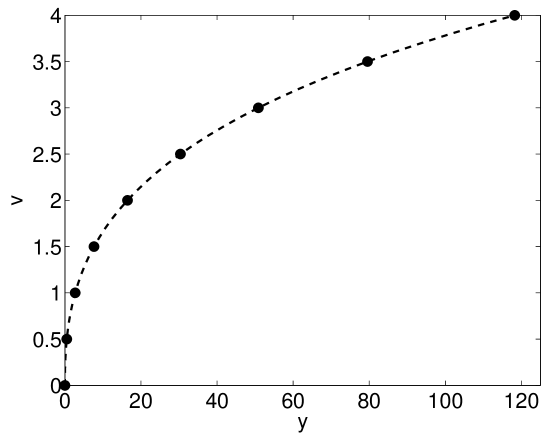
Figure 1: Solution of $v_{y}(1+4v^{3/2}\exp(\frac{1}{2}\sqrt{v}))=2\sqrt{v}$,

-  -  -  -	exact solution,
●	discrete solution.

4.1.2 One Dimensional Linear Heat Equation

The one dimensional linear heat equation

$$u_{t}=u_{xx}$$ (38ao)

admits an infinite dimensional group of Lie point symmetries generated by ,[19],

$$\eqalign{\mathbf{V}_{1}=\partial_{x},\qquad\mathbf{V}_{2}=\partial_{t},\qquad\mathbf{V}_{3}=u\partial_{u},\qquad\mathbf{V}_{4}=x\partial_{x}+2t\partial_{t},\\ \mathbf{V}_{5}=2t\partial_{x}-xu\partial_{u},\qquad\mathbf{V}_{6}=4tx\partial_{x}+4t^{2}\partial_{t}-(x^{2}+2t)u\partial_{u},}$$ (38apa)

$$\mathbf{V}_{\alpha}=\alpha(x,t)\partial_{u}\qquad\mathchoice{\hbox{{where}}}{\hbox{{\firstchoice@false where}}}{\hbox{{\firstchoice@false where}}}{\hbox{{\firstchoice@false where}}}\qquad\alpha_{t}=\alpha_{xx}.$$ (38apb)

To discretize (38ao), we need two discrete indices, $(m,n)\in\mathbb{Z}^{2}$.

To perform our invariant discretisation procedure of the heat equation we consider only the six dimensional Lie algebra (38apa). Before computing the invariants of (38apa), we point out the important fact that

$$\Delta t_{+}=0$$ (38apaq)

is an invariant manifold of (38apa), which we will take to be one of our equations describing the lattice. Hence, the invariants are to be computed on a grid with flat time layers. This restriction is important since we want to be able, at any time iteration, to move everywhere in the spatial domain.

The invariants are computed on a scheme involving the points $(x,t,u)$, $(x_{\pm},t,u_{\pm})$ and $(\hat{x},\hat{t},\hat{u})$. This is the minimum of point necessary to approximate the derivatives present in the heat equation and generate an explicit scheme. The set of elementary invariants is obtained by solving the system of linear partial differential equations

$$\mathbf{pr}\;\mathbf{V}_{k}[I(x,t,u,x_{+},u_{+},x_{-},u_{-},\hat{x},\hat{t},\hat{u})]=0,\qquad k=1,\ldots,6,$$ (38apar)

where the quantity $I$ is supposed to depend on the discrete points involved in the scheme and the $\mathbf{V}_{k}$ are given in (38apa). The solution of (38apar), by the method of characteristics, gives the set of elementary invariants, [21],

$$\eqalign{I_{1}=\frac{\Delta x_{+}}{\Delta x_{-}},\qquad I_{2}=\frac{\Delta x_{+}^{2}}{\hat{\Delta t}}\left(\frac{u}{\hat{u}}\right)^{2}\exp\left[\frac{-\hat{\Delta x}^{2}}{2\hat{\Delta t}}\right],\\ I_{3}=\frac{\Delta x_{+}^{2}}{4\hat{\Delta t}}-\frac{\Delta x_{+}^{2}}{\Delta x_{+}+\Delta x_{-}}\left\{\frac{1}{\Delta x_{+}}\ln\left(\frac{u_{+}}{u}\right)+\frac{1}{\Delta x_{-}}\ln\left(\frac{u_{-}}{u}\right)\right\},\\ I_{4}=\frac{\Delta x_{+}\hat{\Delta x}}{\hat{\Delta t}}+\frac{2\Delta x_{+}}{\Delta x_{+}+\Delta x_{-}}\left\{\frac{\Delta x_{-}}{\Delta x_{+}}\ln\left(\frac{u_{+}}{u}\right)-\frac{\Delta x_{+}}{\Delta x_{-}}\ln\left(\frac{u_{-}}{u}\right)\right\},\\ }$$ (38apas)

The number of elementary invariants is coherent with the formula (10). Indeed, since the scheme involves the points $(x,t,u)$, $(x_{\pm},t,u_{\pm})$ and $(\hat{x},\hat{t},\hat{u})$, the manifold $M$ introduce in equation (10) is given by $M\sim\{x,t,u,x_{+},u_{+},x_{-},u_{-},\hat{x},\hat{t},\hat{u}\}$ so dim $M$=10. Furthermore, since the prolongation of the 6 vector fields given in (38apa) are independent we get from (10), $\mu=10-6=4$.

From the set (38apas) and the weakly invariant equation (38apaq) we define the explicit invariant scheme

$$I_{2}=4I_{3},\qquad\Delta t_{+}=0,\qquad I_{4}=0,$$ (38apat)

which gives in terms of the original variables

$$\left(\frac{u}{\hat{u}}\right)^{2}\exp\left[-\frac{\hat{\Delta x}^{2}}{2\hat{\Delta t}}\right]=1-\frac{4\hat{\Delta t}}{\Delta x_{+}+\Delta x_{-}}\left\{\frac{1}{\Delta x_{+}}\ln\left(\frac{u_{+}}{u}\right)+\frac{1}{\Delta x_{-}}\ln\left(\frac{u_{-}}{u}\right)\right\},$$ (38apaua)

$$\Delta t_{+}=0,$$ (38apaub)

$$\hat{\Delta x}=\frac{2\hat{\Delta t}}{\Delta x_{+}+\Delta x_{-}}\left\{\frac{\Delta x_{+}}{\Delta x_{-}}\ln\left(\frac{u_{-}}{u}\right)-\frac{\Delta x_{-}}{\Delta x_{+}}\ \ln\left(\frac{u_{+}}{u}\right)\right\}.$$ (38apauc)

Notice that the invariant scheme is not linear even though the PDE is. This is due to the fact that we have neglected, in our derivation of the discrete invariants (38apas), the infinite dimensional symmetry generator (38apb), which states that to any solution of the heat equation we can add another solution.

Let us prove that the system of equations (38apaua), (38apaub) and (38apauc) is a valid approximation of the heat equation (38ao) by computing its continuous limit.

We first start by taking the continuous limit in the discrete variable $n$, meaning that $\Delta x_{\pm}$ and $\Delta t_{+}$ go to zero. By doing so, the equations (38apaua), (38apaub) and (38apauc) go to

$$\left(\frac{u}{\hat{u}}\right)^{2}\exp\left[-\frac{\hat{\Delta x}^{2}}{2\hat{\Delta t}}\right]=1-2\hat{\Delta t}\left(\frac{u_{xx}}{u}-\left(\frac{u_{x}}{u}\right)^{2}\right),$$ (38apauava)

$$0=0,$$ (38apauavb)

$$\hat{\Delta x}=-2\hat{\Delta t}\frac{u_{x}}{u},$$ (38apauavc)

respectively. The development of (38apauava) in Taylor series in term of $\hat{\Delta x}$ and $\hat{\Delta t}$ gives, if we keep only the terms that don’t go to zero in the continuous limit,

$$-2\frac{\sigma}{\tau}\frac{u_{x}}{u}-2\frac{u_{t}}{u}-\frac{1}{2}\frac{\sigma^{2}}{\tau^{2}}=-2\frac{u_{xx}}{u}+2\left(\frac{u_{x}}{u}\right)^{2},$$ (38apauavaw)

Using (38apauavc), we replace the occurances of $\hat{\Delta x}$ by $\hat{\Delta t}$ in (38apauavaw) and take the limit $\hat{\Delta t}$ and $\hat{\Delta x}$ to zero. Doing so, the equation (38apauavaw) goes to the heat equation while (38apauavc) goes to $0=0$.

It can be shown, [21], that

$$u(x,t)=\frac{1}{\sqrt{4\pi t}}e^{-x^{2}/4t}, \qquad t=\tau\;m+t_{0}, \qquad x=(h\;n+x_{0})(\tau\;m+t_{0}),$$

$$u(x,t)=Ke^{-cx+c^{2}t}, \qquad t=\tau\;m+t_{0}, \qquad x=h\;n+x_{0}+2c(\tau\;m+t_{0}),$$ (38apauavax)

where $K$, $h$, $x_{0}$, $t_{0}$ $\tau$ and $c$ are constants, are non-trivial exact solutions of the invariant scheme composed of the equations (38apaua), (38apaub) and (38apauc).

Now let us perform the pure hodograph transformation $H:\mathbb{R}^{3}\to\mathbb{R}^{3}$, $(x,t,u)\mapsto(y=u,t,v=x)$. Under such a transformation, the heat equation maps to the nonlinear equation

$$v_{t}=\frac{v_{yy}}{v^{2}_{y}}.$$ (38apauavay)

The symmetry generators of this equation are, [20]

$$\eqalign{\widetilde{\mathbf{V}}_{1}=\partial_{v},\qquad\widetilde{\mathbf{V}}_{2}=\partial_{t},\qquad\widetilde{\mathbf{V}}_{3}=y\partial_{y},\qquad\widetilde{\mathbf{V}}_{4}=v\partial_{v}+2t\partial_{t},\\ \widetilde{\mathbf{V}}_{5}=2t\partial_{v}-vy\partial_{y},\qquad\widetilde{\mathbf{V}}_{6}=4tv\partial_{v}+4t^{2}\partial_{t}-(v^{2}+2t)y\partial_{y},}$$ (38apauavaza)

$$\widetilde{\mathbf{V}}_{\alpha}=\alpha(v,t)\partial_{y}\qquad\mathchoice{\hbox{{where}}}{\hbox{{\firstchoice@false where}}}{\hbox{{\firstchoice@false where}}}{\hbox{{\firstchoice@false where}}}\qquad\alpha_{t}=\alpha_{vv}.$$ (38apauavazb)

Clearly, since $t$ is unaffected by the hodograph transformation, the expression $\Delta t_{+}=0$ will remain an invariant manifold of the new symmetry algebra. The discrete invariants on such an invariant manifold are obtained directly from (38apas), we just perform the hodograph transformation on the set of invariants. Hence we obtain, [21]

$$\eqalign{\widetilde{I}_{1}=\frac{v_{+}-v}{v-v_{-}},\qquad\widetilde{I}_{2}=\frac{(v_{+}-v)^{2}}{\hat{\Delta t}}\left(\frac{y}{\hat{y}}\right)^{2}\exp\left[\frac{-(\hat{v}-v)^{2}}{2\hat{\Delta t}}\right],\\ \widetilde{I}_{3}=\frac{(v_{+}-v)^{2}}{4\hat{\Delta t}}-\frac{(v_{+}-v)^{2}}{v_{+}-v_{-}}\left\{\frac{1}{v_{+}-v}\ln\left(\frac{y_{+}}{y}\right)+\frac{1}{v-v_{-}}\ln\left(\frac{y_{-}}{y}\right)\right\},\\ \widetilde{I}_{4}=\frac{(v_{+}-v)(\hat{v}-v)}{\hat{\Delta t}}+\frac{2(v_{+}-v)}{v_{+}+v_{-}}\left\{\frac{v-v_{-}}{v_{+}-v}\ln\left(\frac{y_{+}}{y}\right)-\frac{v_{+}-v}{v-v_{-}}\ln\left(\frac{y_{-}}{y}\right)\right\},}$$ (38apauavazba)

Using the same invariant expressions as for the discrete heat equation, i.e.

$$\widetilde{I}_{2}=4\widetilde{I}_{3},\qquad\Delta t_{+}=0,\qquad\widetilde{I}_{4}=0,$$ (38apauavazbb)

we get the explicit invariant scheme for (38apauavay),

$$\left(\frac{y}{\hat{y}}\right)^{2}\exp\left[-\frac{(\hat{v}-v)^{2}}{2\hat{\Delta t}}\right]=1-\frac{4\hat{\Delta t}}{v_{+}-v_{-}}\left\{\frac{1}{v_{+}-v}\ln\left(\frac{y_{+}}{y}\right)+\frac{1}{v-v_{-}}\ln\left(\frac{y_{-}}{y}\right)\right\},$$ (38apauavazbca)

$$\Delta t_{+}=0,$$ (38apauavazbcb)

$$\frac{\hat{v}-v}{\hat{\Delta t}}=\frac{2}{v_{+}-v_{-}}\left\{\frac{v_{+}-v}{v-v_{-}}\ln\left(\frac{y_{-}}{y}\right)-\frac{v-v_{-}}{v_{+}-v}\ln\left(\frac{y_{+}}{y}\right)\right\}$$ (38apauavazbcc)

The computation of the continuous limit of (38apauavazbca), (38apauavazbcb) and (38apauavazbcc) is similar to the case of the heat equation. Firstly, by letting the steps generated by the discrete variable $n$ go to zero we get respectively for equation (38apauavazbca), (38apauavazbcb) and (38apauavazbcc)

$$\left(\frac{y}{\hat{y}}\right)^{2}\exp\left[-\frac{2\hat{\Delta t}}{y^{2}v_{y}^{2}}\right]=1+2\hat{\Delta t}\left(\frac{v_{yy}}{yv_{y}^{3}}+\frac{1}{y^{2}v_{y}^{2}}\right)$$ (38apauavazbcbda)

$$0=0$$ (38apauavazbcbdb)

$$\frac{\hat{v}-v}{\hat{\Delta t}}=-\frac{2}{yv_{y}}$$ (38apauavazbcbdc)

By developping the two nontrivial equations in Taylor series with respect to the step generated by the discrete variable $m$ we get

$$\frac{\hat{\Delta y}}{\hat{\Delta t}}v_{y}+v_{t}+\mathcal{O}(\frac{\hat{\Delta y^{2}}}{\hat{\Delta t}},\hat{\Delta t},\hat{\Delta y})=-\frac{2}{yv_{y}}$$ (38apauavazbcbdbea)

$$\hat{\Delta y}=-\hat{\Delta t}\left(\frac{v_{yy}}{v_{y}^{3}}+\frac{2}{yv_{y}^{2}}\right).$$ (38apauavazbcbdbeb)

By replacing the appearances of $\hat{\Delta y}$ in terms of $\hat{\Delta t}$ in (38apauavazbcbdbea) with the help of (38apauavazbcbdbeb) and then taking the limit $\hat{\Delta y}$ and $\hat{\Delta t}$ to zero we recover from (38apauavazbcbdbea) the PDE (38apauavay) while (38apauavazbcbdbeb) goes to $0=0$.

Finally, by a direct substitution we can verify that the exact solutions of the linear heat equation, (38apauavax), are again solutions of the invariant schemes of the nonlinear partial differential equation (38apauavay), after performing the hodograph transformation on them. Namely, we have that

$$v=(h\;n+v_{0})(\tau\;m+t_{0}), \qquad t=\tau\;m+t_{0}, \qquad y=\frac{1}{\sqrt{4\pi t}}e^{-v^{2}/4t},$$

$$v=h\;n+v_{0}+2c(\tau\;m+t_{0}), \qquad t=\tau\;m+t_{0}, \qquad y=Ke^{-cv+c^{2}t},$$ (38apauavazbcbdbebf)

are exact solutions of the invariant system composed of equations (38apauavazbca), (38apauavazbcb) and (38apauavazbcc), where $K$, $h$, $v_{0}$, $t_{0}$, $\tau$ and $c$ are constants.

From this last example, we notice that even though a pure hodograph transformation can linearize a differential equation, it does not mean that the transformation on a discrete invariant scheme will have the same effect. Indeed, the inverse hodograph transformation can be use to transform the nonlinear equation (38apauavay) to (38ao). However, since the invariant scheme of the latter is not linear, the discrete invariant scheme for $v_{t}=v_{y}^{-2}v_{yy}$ will not be linearized.

4.2 (1+1) dimensional wave equation with a source term

In this section we obtain a symmetry-preserving scheme of the (1+1) dimensional wave equation

$$u_{tt}-u_{xx}=-4F(u),$$ (38apauavazbcbdbebg)

where $F(u)$ is an arbitrary function of $u$. The symmetry algebra of (38apauavazbcbdbebg) is generated by

$$\mathbf{V}_{1}=t\partial_{x}+x\partial_{t},\qquad\mathbf{V}_{2}=\partial_{x},\qquad\mathbf{V}_{3}=\partial_{t}.$$ (38apauavazbcbdbebh)

instead of finding an invariant scheme in the space $\{x,t,u\}$ we make the change of coordinates to the characteristic variables

$$\psi:\mathbb{R}^{2}\to\mathbb{R}^{2},\qquad(x,t)\mapsto(y,z)=(x+t,x-t).$$ (38apauavazbcbdbebi)

Under the transformation (38apauavazbcbdbebi), the PDE (38apauavazbcbdbebg) is mapped to

$$u_{yz}=F(u).$$ (38apauavazbcbdbebj)

A basis of the Lie symmetry algebra of (38apauavazbcbdbebj) is

$$\widetilde{\mathbf{V}}_{1}=y\partial_{y}-z\partial_{z},\qquad,\widetilde{\mathbf{V}}_{2}=\partial_{y},\qquad\widetilde{\mathbf{V}}_{3}=\partial_{z},$$ (38apauavazbcbdbebk)

where $\widetilde{\mathbf{V}}_{2}=1/2(d\psi(\mathbf{V}_{2}+\mathbf{V}_{3}))$ and $\widetilde{\mathbf{V}}_{3}=1/2(d\psi(\mathbf{V}_{2}-\mathbf{V}_{3}))$.

Before computing any invariants we have that

$$\hat{y}-y=0,\qquad z_{+}-z=0$$ (38apauavazbcbdbebl)

are two weakly invariant equations of the symmetry algebra (38apauavazbcbdbebk) since they verify the condition (13). By including these two equations in our invariant scheme we can compute the invariants on an orthogonal lattice, figure 2.

Figure 2: Invariant lattice of equation (38apauavazbcbdbebj).

A basis of elementary invariants in the space of discrete points $\{(y,\hat{z},\hat{u}),$ $(y,z,u),$ $(y,\check{z},\check{u}),$ $(y_{+},z,u_{+}),$ $(y_{-},z,u_{+}),$ $(y_{+},\hat{z}_{+},\hat{u}_{+})\}$ is

$$\eqalign{\widetilde{I}_{1}=u,\quad\widetilde{I}_{2}=u_{+},\quad\widetilde{I}_{3}=u_{-},\quad\widetilde{I}_{4}=\check{u},\widetilde{I}_{5}=\hat{u},\quad\widetilde{I}_{6}=\hat{u}_{+},\\ \widetilde{I}_{7}=\frac{\Delta y_{+}}{\Delta y_{-}},\quad\widetilde{I}_{8}=\frac{\hat{\Delta y}_{+}}{\Delta y_{+}},\quad\widetilde{I}_{9}=\frac{\hat{\Delta z}}{\check{\Delta z}},\quad\widetilde{I}_{10}=\Delta y_{+}\hat{\Delta z},}$$ (38apauavazbcbdbebm)

where $\hat{\Delta y}_{+}=\hat{y}_{+}-\hat{y}$.

From this set of invariants we generate a symmetry-preserving scheme by setting

$$\frac{\widetilde{I}_{6}-\widetilde{I}_{5}}{\widetilde{I}_{8}\widetilde{I}_{10}}-\frac{\widetilde{I}_{2}-\widetilde{I}_{1}}{\widetilde{I}_{10}}=F(\widetilde{I}_{1}),$$ (38apauavazbcbdbebna)

$$\hat{y}-y=0,\qquad z_{+}-z=0.$$ (38apauavazbcbdbebnb)

The equations for the lattice, (38apauavazbcbdbebnb), can be solved and give

$$y=\epsilon(m)\;n+y_{0}(m),\qquad z=\delta(n)\;m+z_{0}(n).$$

From (38apauavazbcbdbebm) we see that it is also possible to impose $\Delta y_{+}=\Delta y_{-}$, by setting $\widetilde{I}_{7}=1$ and $\hat{\Delta z}=\check{\Delta z}$ by setting $\widetilde{I}=1$ without loosing any symmetries. So if we do so, the final solution for the lattice is

$$y=\epsilon\;n+y_{0},\qquad z=-\delta\;m-z_{0},$$ (38apauavazbcbdbebnbo)

where $\epsilon$, $y_{0}$, $\delta$ and $z_{0}$ are constants. On this rectangular lattice, the equation (38apauavazbcbdbebna) becomes in term of the discrete variables

$$\frac{\hat{u}_{+}-\hat{u}-u_{+}+u}{\epsilon\delta}=F(u),$$ (38apauavazbcbdbebnbp)

which correspond to a standard discretisation of (38apauavazbcbdbebg). The interesting thing to do now is to come back to the original variables $\{x,t,u\}$ by applying the inverse transformation of (38apauavazbcbdbebi)

$$\psi^{-1}(x,t)=(\frac{1}{2}(y+z),\frac{1}{2}(y-z)).$$ (38apauavazbcbdbebnbq)

First of all, the invariant equations (38apauavazbcbdbebl) become

$$\hat{\Delta x}=-\hat{\Delta t},\qquad\Delta x_{+}=\Delta t_{+}.$$ (38apauavazbcbdbebnbr)

The equations (38apauavazbcbdbebnbr) are weakly invariant equations of (38apauavazbcbdbebh) and are chosen to be part of the invariant scheme of (38apauavazbcbdbebg). The basis of invariants (38apauavazbcbdbebm) on the invariant manifold (38apauavazbcbdbebnbr) becomes

$$\eqalign{I_{1}=u,\quad I_{2}=u_{+},\quad I_{3}=u_{-},\quad I_{4}=\check{u},\quad I_{5}=\hat{u},\quad I_{6}=\hat{u}_{+},\\ I_{7}=\frac{\Delta x_{+}}{\Delta x_{-}},\quad I_{8}=\frac{\hat{\Delta x}_{+}}{\Delta x_{+}},\quad I_{9}=\frac{\hat{\Delta t}}{\check{\Delta t}},\quad I_{10}=-4\Delta x_{+}\hat{\Delta t},}$$ (38apauavazbcbdbebnbs)

under the transformation (38apauavazbcbdbebnbq). By setting the same combination of invariants as in (38apauavazbcbdbebna) and (38apauavazbcbdbebnb) and adding the equations $I_{7}=1$ and $I_{9}=1$ we get an invariant scheme of (38apauavazbcbdbebg)

$$\eqalign{\frac{I_{6}-I_{5}}{I_{8}I_{10}}-\frac{I_{2}-I_{1}}{I_{10}}=F(I_{1}),\\ \hat{\Delta x}=-\hat{\Delta t},\quad\Delta x_{+}=\Delta t_{+},\quad I_{7}=1,\quad I_{9}=1.}$$ (38apauavazbcbdbebnbt)

Which gives in term of the original variables

$$\frac{\hat{u}_{+}\hat{u}}{\hat{\Delta x}_{+}\hat{\Delta t}}-\frac{u_{+}-u}{\Delta x_{+}\hat{\Delta t}}=-4F(u),$$ (38apauavazbcbdbebnbua)

$$\hat{\Delta x}=-\hat{\Delta t},\qquad\hat{\Delta t}=\check{\Delta t},$$ (38apauavazbcbdbebnbub)

$$\Delta x_{+}=\Delta x_{-},\qquad\Delta x_{+}=\Delta t_{+},$$ (38apauavazbcbdbebnbuc)

where $\hat{\Delta x}_{+}=\hat{x}_{+}-\hat{x}$. The solution for the lattice is obtain from the known solution for the mesh in $y$ and $z$ and using the transformation (38apauavazbcbdbebnbq)

$$x=\frac{1}{2}(\epsilon\;n+y_{0}-\delta\;m-z_{0}),\qquad t=\frac{1}{2}(\epsilon\;n+y_{0}+\delta\;m+z_{0}).$$ (38apauavazbcbdbebnbubv)

The solution for the mesh (38apauavazbcbdbebnbubv) is drawn in figure 3.

Figure 3: Invariant lattice of equation (38apauavazbcbdbebg).

We compute the continuous to show that the finite difference equation (38apauavazbcbdbebnbua) is a valid approximation of the partial differential equation (38apauavazbcbdbebg) on the lattice given by (38apauavazbcbdbebnbubv). Taking into account that the lattice implies

$$\Delta x_{+}=\Delta t_{+}\qquad\mathchoice{\hbox{{and}}}{\hbox{{\firstchoice@false and}}}{\hbox{{\firstchoice@false and}}}{\hbox{{\firstchoice@false and}}}\qquad\hat{\Delta x}_{+}=\Delta x_{+},$$ (38apauavazbcbdbebnbubw)

we find by taking the Taylor series in the steps involving the variation of the discrete variable $n$ of (38apauavazbcbdbebnbua) that

$$\eqalign{\left\{\hat{u}_{x}+\hat{u}_{t}+\frac{\Delta x_{+}}{2}(\hat{u}_{xx}+\hat{u}_{tt}+2\hat{u}_{xt})+\mathcal{O}(\Delta x_{+}^{2})\right.\\ \left.-\left(u_{x}+u_{t}+\frac{\Delta x_{+}}{2}(u_{xx}+u_{tt}+2u_{xt})+\mathcal{O}(\Delta x_{+}^{2})\right)\right\}\frac{1}{\hat{\Delta t}}=-4F(u),}$$ (38apauavazbcbdbebnbubx)

where the hat over the derivatives of $u$ means that they are evaluated at $(\hat{x},\hat{t})$. By developping the hat derivatives around $(x,t)$ we get

$$u_{tt}-u_{xx}+\mathcal{O}(\Delta x_{+},\hat{\Delta t})=-4f(u),$$ (38apauavazbcbdbebnbuby)

which goes to the desired limit when $\Delta x_{+}$ and $\hat{\Delta t}$ go to zero.

The invariant discretisation (38apauavazbcbdbebnbua) of (38apauavazbcbdbebg) is quite different from the standard discretisation

$$\eqalign{\frac{u_{+}-2u+u_{-}}{\epsilon^{2}}-\frac{\hat{u}-2u+\check{u}}{\delta^{2}}=-4F(u),\\ x=\epsilon\;n+x_{0},\qquad t=\delta\;m+t_{0}.}$$

The difference is due to the counterclockwise rotation of 45 degrees of the rectangular lattice in the invariant case.

4.3 Polar coordinates transformation

A more interesting transformation of coordinates to be considered is the passage for cartesian to polar coordinates. Unlike the other examples the two spaces of variables are different since the metric is not the same for each space.

We consider the elliptic partial differential equation

$$u_{xx}+u_{yy}=F(u,x^{2}+y^{2}),$$ (38apauavazbcbdbebnbubz)

where $F$ is an arbitrary function. The only symmetry of (38apauavazbcbdbebnbubz) is the invariance under rotation

$$\mathbf{V}=-y\partial_{x}+x\partial_{y}.$$ (38apauavazbcbdbebnbuca)

Nevertheless it is not obvious how to discretize (38apauavazbcbdbebnbubz) in cartesian coordinates and preserve the rotationnal symmetry. The natural thing to do is to pass to polar coordinates

$$x=r\cos\theta,\qquad y=r\sin\theta.$$ (38apauavazbcbdbebnbucb)

In polar coordinates the equation (38apauavazbcbdbebnbubz) becomes

$$u_{rr}+\frac{1}{r}u_{r}+\frac{1}{r^{2}}u_{\theta\theta}=F(u,r)$$ (38apauavazbcbdbebnbucc)

and (38apauavazbcbdbebnbuca) becomes the generator of translation in $\theta$

$$\widetilde{\mathbf{V}}=\partial_{\theta}.$$ (38apauavazbcbdbebnbucd)

Without going through the whole algorithm for finding an invariant scheme, it is clear that the standard discretisation of (38apauavazbcbdbebnbucc)

$$\eqalign{\frac{u_{+}-2u+u_{-}}{\epsilon^{2}}+\frac{1}{r}\frac{u_{+}-u}{\epsilon}+\frac{1}{r^{2}}\frac{\hat{u}-2u+\check{u}}{\delta^{2}}=F(u,r),\\ \hat{r}-r=0,\quad r_{+}-r=\epsilon,\quad\theta_{+}-\theta=0,\quad\hat{\theta}-\theta=\delta,}$$ (38apauavazbcbdbebnbuce)

is invariant under translation in theta since it only involves the difference between two values of theta. The solution for the lattice is given by

$$r=\epsilon\;n+r_{0},\qquad\theta=\delta\;m+\theta_{0}.$$ (38apauavazbcbdbebnbucf)

where $\epsilon$, $\delta$, $r_{0}$ and $\theta_{0}$ are constants.

Now, if we go back to cartesian coordinates

$$r=\sqrt{x^{2}+y^{2}},\qquad\theta=\arctan\left(\frac{y}{x}\right),$$

the invariant scheme (38apauavazbcbdbebnbuce) becomes

$$\eqalign{\frac{u_{+}-2u+u_{-}}{\epsilon^{2}}+\frac{1}{\sqrt{x^{2}+y^{2}}}\frac{u_{+}-u}{\epsilon}+\frac{1}{x^{2}+y^{2}}\frac{\hat{u}-2u+\check{u}}{\delta^{2}}=F(u,\sqrt{x^{2}+y^{2}}),\\ \sqrt{\hat{x}^{2}+\hat{y}^{2}}-\sqrt{x^{2}+y^{2}}=0,\quad\sqrt{x_{+}^{2}+y_{+}^{2}}-\sqrt{x^{2}+y^{2}}=\epsilon,\\ \arctan\bigg{(}\frac{y_{+}}{x_{+}}\bigg{)}-\arctan\bigg{(}\frac{y}{x}\bigg{)}=0,\quad\arctan\bigg{(}\frac{\hat{y}}{\hat{x}}\bigg{)}-\arctan\bigg{(}\frac{y}{x}\bigg{)}=\delta,}$$ (38apauavazbcbdbebnbucg)

and is invariant under (38apauavazbcbdbebnbuca). From (38apauavazbcbdbebnbucb) and (38apauavazbcbdbebnbucf) we have that the lattice in the $x$, $y$ variables is given by

$$x=(\epsilon\;n+r_{0})\cos(\delta\;m+\theta_{0}),\qquad y=(\epsilon\;n+r_{0})\sin(\delta\;m+\theta_{0}).$$ (38apauavazbcbdbebnbuch)

In the Fig. 4 we have illustrated the lattice. By carefully taking continuous limit of (38apauavazbcbdbebnbucg) on the lattice (38apauavazbcbdbebnbuch) we obtain, as expected, the PDE (38apauavazbcbdbebnbubz).

Figure 4: Invariant lattice of equation (38apauavazbcbdbebnbubz),

●	discrete points involved in (38apauavazbcbdbebnbucg),
○	other discrete points.

Conclusion

It is a well known fact that if the symmetry groups of two systems of differential equations are related by a point transformation then these two systems are mapped into each other by the same point transformation. In this work, we have shown that same result is true for invariant schemes. That is, given a system of differential equations and its invariant scheme, any point transformation will map the system of differential equations to a new system and the invariant scheme to a new invariant scheme of the new system. This result has been used to derive new invariant schemes of differential equations from known ones, section 4.1. We have obtained exact solutions of these new schemes by applying the point transformation to known solutions. In section 4.2 and 4.3, we have seen that a change of coordinates can be used to facilitate the computation of an invariant scheme of a differential equation.

The validity of the results obtained in this article rely heavily on the point aspect of the transformation $\psi$. The result does not apply to nonlocal transformations since such transformations will inevitably break the local character of the symmetry transformations.

References

References

- [1] Hairer E, Lubich C and Wanner G 2002 Geometric Numerical Integration (New York:Springer-Verlag)
- [2] Floreanini R, Negro J, Nieto L M and Vinet L 1996 J. Math. Phys. 36 351–5
- [3] Levi D, Vinet, L and Winternitz P 1997 J. Phys. A: Math. Gen. 30 633–49
- [4] Levi D, Tempesta P and Winternitz P 2004 J. Math. Phys. 45, 4077-105
- [5] Kim P and Olver P J 2004 Regular and Chaotic Dynamics 9 213–26
- [6] Olver P J 2001 Appl. Alg. Engin. Comp. Commun. 11 417–36
- [7] Dorodnitsyn V A and Kozlov R 2003 J. Non. Math. Phys 10 16–50
- [8] Dorodnitsyn V, Kozlov R and Winternitz P 2000 J. Math. Phys. 41 480–504
- [9] Dorodnitsyn V, Kozlov R and Winternitz P 2004 J. Math. Phys. 45 336–59
- [10] Rodiguez M A and Winternitz P 2004 J. Phys. A: Math. Gen. 37 6129–42
- [11] Lie S 1893 Vorlesungen über Continuirliche Gruppen mit Geometrischen und Anderen Anwendungen, Bearbeited und Herausgegeben von Dr. G. Scherffers (Leipzig:Taubner)
- [12] Lie S 1893 Theorie Der Transformationsgruppen, Dritter Abschnitt, Abteilun. I. Unter Mitwirkung von Pr. F. Engel (Leipzig:Taubner)
- [13] Dorodnitsyn V A, J. Sov. Math. 55 1490–517
- [14] Levi D and Winternitz P 1991 Phys. Lett. A 152 335–8
- [15] Levi D and Winternitz P 2005 Preprint arXiv:nlin/0502004 s
- [16] Dorodnitsyn V A and Kozlov R 1997 Preprint SYNODE preprint Numerics No. 4
- [17] Levi D, Tremblay S and Winternitz P 2001 J. Phys. A: Math. Gen. 34 9507–24
- [18] Ames W F 1996 Nonlinear Partial Differential Equations in Engineering (New York:Academic Press)
- [19] Olver P J 1993 Applications of Lie Groups to Differential Equations (New York:Springer Verlag)
- [20] Olver P J 1995 Equivalence, Invariants, and Symmetries (New York:Cambridge University Press)
- [21] Valiquette F 2005 Discrétisation des équations différentielles aux dérivées partielles avec préservation de leurs symétries (Master Thesis, University of Montréal)