Discretizations preserving all Lie point symmetries of the Korteweg-de Vries equation

Abstract

• † Centre de Recherches Mathématiques, Université de Montréal, C.P. 6128, succ. Centre-ville, Montréal, QC, H3C 3J7, Canada

• Abstract. We show how to descritize the Korteweg-de Vries (KdV) equation in such a way as to preserve all the Lie point symmetries of the continuous differential equation. It is shown that, for a centered implicit scheme, there are at least two possible ways of doing so.

• † Centre de Recherches Mathématiques, Université de Montréal, C.P. 6128, succ. Centre-ville, Montréal, QC, H3C 3J7, Canada

• Abstract. We show how to descritize the Korteweg-de Vries (KdV) equation in such a way as to preserve all the Lie point symmetries of the continuous differential equation. It is shown that, for a centered implicit scheme, there are at least two possible ways of doing so.

  1 Introduction

  Symmetries play an important role in our understanding of nature, they are intrinsic and fundamental features of differential equations in mathematical physics. Hence, they should be retained when discrete analogs of such equations are constructed. The aim of this paper is to give a systematic approach for discretizing partial differential equations (PDEs), involving one function of two variables $u(x,t)$, such that all the Lie point symmetries of the original problem are preserved. To illustrate the procedure we investigate the case of the KdV equation. We will show how it is possible to obtain invariant implicit schemes. Explicit schemes can also be derived but they often exhibit numerical instability. Finally, a numerical application is realized using the schemes obtained.

  2 Discretization procedure

  The discretization of a PDE involving one depend variable $u$ and two independant ones, $x$ and $t$, consists of sampling, couples $(x,t)$ in the real plane. Each point is labelled by a set of discrete indices:

  $$(x_{m,n},t_{m,n}),\qquad m,n\in\mathbb{Z}.$$ (1)

  The discretization of the independant variables induces a natural discretization of the dependant one

  $$u_{m,n}=u(x_{m,n},t_{m,n}).$$ (2)

  A two-variable partial difference scheme (P$\Delta$S) approximating the original PDE will be a set of three equations relating the quantities $\{x,t,u\}$ at a finite number of points

  $$\left.\begin{aligned} &E_{k}(\{x_{m+i,n+j},t_{m+i,n+j},u_{m+i,n+j}\})=0,\\ &1\leq k\leq 3,\qquad i_{1}\leq i\leq i_{2},\qquad j_{1}\leq j\leq j_{2},\end{aligned}\right.$$ (3)

  such that, in the continous limit, all three equations (3) reduce to the original PDE. By choice, we suppose that $E_{1,2}=0$ describe the lattice and impose that in the continous limit these equations go to the identity $0=0$ while $E_{3}=0$ goes to the PDE. We also require that the system (3) be invariant under the same group of symmetries as the original PDE.

  2.1 Lie point symmetries of P$\Delta$S

  Let $G$ be the group of Lie point symmetries, of order $N$, for a given PDE

  $$\left.\begin{aligned} x^{*}_{l}&=X_{l}(x,t,u,\epsilon)=x+\epsilon\xi^{l}(x,t,u)+\mathop{\rm O}\nolimits(\epsilon^{2})\\ t^{*}_{l}&=T_{l}(x,t,u,\epsilon)=t+\epsilon\tau^{l}(x,t,u)+\mathop{\rm O}\nolimits(\epsilon^{2}),\qquad l=1,\ldots,N\\ u^{*}_{l}&=U_{l}(x,t,u,\epsilon)=u+\epsilon\phi^{l}(x,t,u)+\mathop{\rm O}\nolimits(\epsilon^{2}).\end{aligned}\right.$$ (4)

  To this group is associated the Lie algebra of vector fields

  $$\mathbf{V}_{l}=\xi^{l}(x,t,u)\partial_{x}+\tau^{l}(x,t,u)\partial_{t}+\phi^{l}(x,t,u)\partial_{u},\qquad l=1,\ldots,N.$$ (5)

  As in the continous case, we define a prolongation of (5), but in a different fashion. The prolongation is realized by requiring that the vector field acts at all points figuring in (3):

  $$\text{pr}\mathbf{V}_{l}:=\sum_{i=m+i_{1}}^{m+i_{2}}\sum_{j=n+j_{1}}^{n+j_{2}}[\xi_{ij}^{l}\partial_{x_{ij}}+\tau_{ij}^{l}\partial_{t_{ij}}+\phi_{ij}^{l}\partial_{u_{ij}}]$$ (6)

  where

  $$\xi_{ij}^{l}=\xi^{l}(x_{ij},t_{ij},u_{ij}),\quad\tau_{ij}^{l}=\tau^{l}(x_{ij},t_{ij},u_{ij})\quad\text{and}\quad\phi_{ij}^{l}=\phi^{l}(x_{ij},t_{ij},u_{ij}).$$

  Let $M$ be the manifold on which $G$ acts, i.e. $M\thicksim\{x_{m+i_{1},n+j_{1}},t_{m+i_{1},n+j_{1}},u_{m+i_{1},n+j_{1}},\ldots,$ $x_{m+i_{2},n+j_{2}},t_{m+i_{2},n+j_{2}},u_{m+i_{2},n+j_{2}}\}$. The quantity $I:M\to\mathbb{R}$ is said to be strongly invariant if it satisfies

  $$\text{pr}\mathbf{V}_{l}I=0,\qquad l=1,\ldots,N.$$ (7)

  Using the method of the characteristics, we obtain a set of elementary invariants $\{I_{1},\ldots,I_{\alpha}\}$. The number of them is given by

  $$\alpha=\text{dim }M-\text{rank }Z,\qquad\alpha\geq 0,$$ (8)

  where $Z$ is the $N\times(i_{2}-i_{1}+j_{2}-j_{1})$ matrix

  $$Z=\begin{pmatrix}\xi^{1}_{m+i_{1},n+j_{1}}&\tau^{1}_{m+i_{1},n+j_{1}}&\phi^{1}_{m+i_{1},n+j_{1}}&\ldots&\xi^{1}_{m+i_{2},n+j_{2}}&\tau^{1}_{m-+i_{2},n+j_{2}}&\phi^{1}_{m+i_{2},n+j_{2}}\\ \vdots&\vdots&\vdots&\ddots&\vdots&\vdots&\vdots\\ \xi^{N}_{m+i_{1},n+j_{1}}&\tau^{N}_{m+i_{1},n+j_{1}}&\phi^{N}_{m+i_{1},n+j_{1}}&\ldots&\xi^{N}_{m+i_{2},n+j_{2}}&\tau^{N}_{m+i_{2},n+j_{2}}&\phi^{N}_{m+i_{2},n+j_{2}}\end{pmatrix}.$$ (9)

  A difference equation will be strongly invariant under $G$ if it can be written as

  $$E(I_{1},\ldots,I_{\alpha})=0.$$ (10)

  Other invariant difference equations can be obtain if there exist expressions

  $$E(x_{m+i_{1},n+j_{1}},t_{m+i_{1},n+j_{1}},u_{m+i_{1},n+j_{1}},\ldots,x_{m+i_{2},n+j_{2}},t_{m+i_{2},n+j_{2}},u_{m+i_{2},n+j_{2}})=0$$

  such that the rank of $Z$ is not maximal. Such equations are said to be weakly invariant and satisfy

  $$\text{pr}\mathbf{V}_{l}E\bigg{\lvert}_{E=0}=0,\qquad l=1,\ldots,N.$$ (11)

  3 Discretization of the Korteweg-de Vries equation

  It is well known [2], that the KdV equation

  $$u_{t}=uu_{x}+u_{xxx}$$ (12)

  admits a 4-parameter Lie symmetry group of point transformations, generated by the infinitesimal operators:

  $$\begin{split}\mathbf{V}_{1}=\partial_{x},\qquad\mathbf{V}_{2}=\partial_{t},\qquad\mathbf{V}_{3}=t\partial_{x}-\partial_{u},\\ \mathbf{V}_{4}=x\partial_{x}+3t\partial_{t}-2u\partial_{u}.\qquad\quad\end{split}$$ (13)

  Before computing the strong invariants of (13), we point out the fact that

  $$T_{+}\equiv t_{m,n+1}-t_{m,n}=0$$ (14)

  is a weakly invariant equation. Hence, the strong invariants can be computed on a scheme with flat time layers, which is physically desirable. For numerical stability reasons, we compute the invariants on an implicit scheme involving the points shown below

  For notational simplicity, we write

  $$(x_{m,n},t_{m,n},u_{m,n})\equiv(x,t,u),\;(x_{m+1,n},t_{m+1,n},u_{m+1,n})\equiv(\hat{x},\hat{t},\hat{u}),\;(x_{m,n\pm 1},t_{m,n\pm 1},u_{m,n\pm 1})\equiv(x_{\pm},t_{\pm},u_{\pm})$$

  and so on. The results of the computations are:

  $$I_{1}=\frac{\hat{h}_{+}}{\hat{h}_{-}}\qquad\;\;I_{2}=\frac{\hat{h}_{++}}{\hat{h}_{+}}\qquad\qquad\;\;I_{3}=\frac{\hat{h}_{-}}{\hat{h}_{--}}\qquad\;\;I_{4}=\frac{\hat{h}_{+}^{3}}{\tau_{+}}$$ (15)

  $$I_{5}=\frac{\sigma+\tau u}{\hat{h}_{+}}\qquad\qquad\qquad\qquad\quad I_{6}=\hat{h}_{+}^{2}(\hat{u}_{+}-u)$$

  $$I_{7}=\tau\hat{u}_{x}^{--}=\tau\left(\frac{\hat{u}_{-}-\hat{u}_{--}}{\hat{h}_{--}}\right)\qquad I_{8}=\tau\hat{u}_{x}^{-}=\tau\left(\frac{\hat{u}-\hat{u}_{-}}{\hat{h}_{-}}\right)$$

  $$I_{9}=\tau\hat{u}_{x}^{+}=\tau\left(\frac{\hat{u}_{+}-\hat{u}}{\hat{h}_{+}}\right)\qquad\quad\;\;I_{10}=\tau\hat{u}_{x}^{++}=\tau\left(\frac{\hat{u}_{++}-\hat{u}_{+}}{\hat{h}_{++}}\right)$$

  From the set of invariants (15), different type of schemes can be obtained. We will restrict our attention to schemes for which the evolution of the solution is given implicitly over a lattice that can be determined explicitly.

  3.1 Lattice with uniform steps in $x$

  $$T_{+}=0$$

  $$I_{1}=1$$ (16)

  $$I_{6}=\frac{1}{2}{(I_{6}+I_{5}I_{4})(I_{9}+I_{8})+(I_{10}-I_{9})-(I_{8}-I_{7})}.$$

  In terms of the original variables, system (16) reduces to

  $$T_{+}=0$$

  $$\hat{h}_{+}=\hat{h}_{-}\equiv\hat{h}$$ (17)

  $$\frac{(\hat{u}-u)}{\tau}=\hat{u}\frac{(\hat{u}_{+}-\hat{u}_{-})}{2\hat{h}}+\frac{(\hat{u}_{++}-2\hat{u}_{+}+2\hat{u}_{-}-\hat{u}_{--})}{2\hat{h}^{3}}+\frac{\sigma}{\tau}\frac{(\hat{u}_{+}-\hat{u}_{-})}{2\hat{h}}.$$

  The third equation of (17) converges in the continuous limit to the KdV equation if

  $$\left\lvert\frac{\sigma}{\tau}\right\rvert\xrightarrow[\tau\to 0]{\sigma\to 0}\lvert R\rvert<\infty.$$ (18)

  Hence $\sigma=\mathop{\rm O}\nolimits(\tau)$. Further more, the equations for the lattice can be solved and give

  $$t_{m,n} =\gamma(m),$$ (19)

  $$x_{m,n} =\alpha(m)n+\beta(m),$$

  where $\gamma(m)$, $\alpha(m)$ and $\beta(m)$ are arbitrary functions that we can choose. The extra term

  $$\frac{\sigma}{\tau}\frac{(\hat{u}_{+}-\hat{u}_{-})}{2\hat{h}}$$

  in the discrete KdV equation is geometrically seen to be a correction term to the solution taking in account the possible displacement of the points in $x$ as the time evolves.

  3.2 Lattice depending on the solution

  Schemes for which the evolution of the lattice depends on the solution have already been obtained by Dorodnitsyn et al , [1]. They use the concept of Lagrangian coordinates which is a point of view that differs from ours. Nevertheless, we get

  $$T_{+}=0$$

  $$I_{5}=0$$ (20)

  $$I_{6}=\frac{6}{I_{2}+2+2I_{1}^{-1}+(I_{3}I_{1})^{-1}}\left\{\frac{I_{10}-I_{9}}{I_{2}+1}-\frac{I_{8}-I_{7}}{I_{3}^{-1}+1}I_{1}\right\}$$

  which in terms of the original variables gives

  $$T_{+}=0$$

  $$\sigma=-\tau u$$ (21)

  $$\frac{\hat{u}-u}{\tau}=\frac{6}{\hat{h}_{++}+2\hat{h}_{+}+2\hat{h}_{-}+\hat{h}_{--}}\left\{\frac{\hat{u}_{x}^{++}-\hat{u}_{x}^{+}}{\hat{h}_{++}+\hat{h}_{+}}-\frac{\hat{u}_{x}^{-}-\hat{u}_{x}^{--}}{\hat{h}_{--}+\hat{h}_{-}}\right\}.$$

  From the numerical point of view, the scheme (21) is interesting since there is no nonlinear term in the equation governing the evolution of the solution. Hence, the computation time is reduced since we avoid nonlinear numerical methods. The absence of the nonlinear term is compensated by the specific evolution of the lattice.

  4 Numerical application

  This section is not meant to be an exhaustive investigation of all the numerical aspects of our invariant schemes. Actually, the aim is to give an illustration of the usefulness of such schemes for computing numerical solutions.

  The solution we have choosen to investigate is

  $$u(x,t)=-\frac{x}{t}.$$ (22)

  Now, if we want to use the scheme (17), we must first specify the lattice over which the numerical solution is to be computed. From all the possible choices, we will look at two specific cases. As a first choice, since (22) is linear in $x$, we may take

  $$x_{m+1,n}-x_{m,n}\equiv\sigma=\tau\frac{x}{t}.$$ (23)

  The solution of (23) is given by

  $$x_{m,n}=h_{0}\left(\frac{t+\tau}{t}\right)^{m}n$$ (24)

  where $h_{0}$ is the initial step in $x$. With this choice, scheme (17) reduces to the scheme (21). As a second choice, we choose $\sigma$ to be zero. In that case, the lattice is orthogonal and the discretization reduces to the standard implicit discretization of the KdV equation.

  

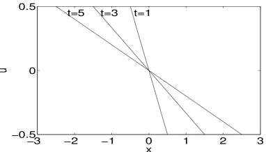
  Figure 1: Numerical solution on the evolutive lattice scheme.

  

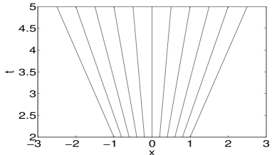
  Figure 2: Evolution of the lattice.

  

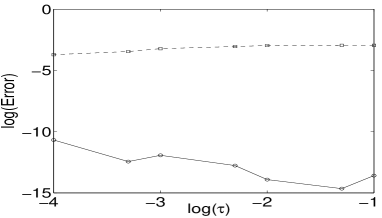
  Figure 3: Evolution of the error as a fonction of $\tau$: $h(t_{0})=0.1$, —— evolutive lattice, – – – orthogonal lattice.

  

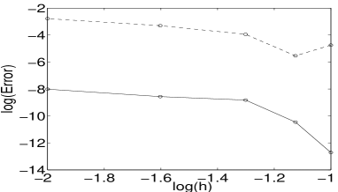
  Figure 4: Evolution of the error as a fonction of $h_{0}$: $\tau=0.000001$ —— evolutive lattice, – – – orthogonal lattice.

  In the Figures 2 and 2 we have plotted the evolution of the solution and lattice for the scheme define on the evolutive grid. The initial step in $x$ was $h_{0}=0.1$ and in the time variable, we’ve taken a constant step, $\tau=0.1$.

  We’ve also plotted the evolution of the error as a fonction of the step sizes in the figures 4 and 4 for the two schemes choosen. The error has been computed using the $l_{\infty}$ norm. As it can be seen, the error due to the evolutive lattice is much smaller than the one generated with the orthogonal mesh.

  From this numerical simulation, we clearly see, that for the scheme (17), the choice of the lattice influences a lot the numerical precision. At the moment, we don’t have a systematic way of determining the lattice that will give the best numerical results. On the other hand, with the scheme (21) everything is determined by the system. The only unknowns are the initial steps in $x$ and those in $t$.

  5 Conclusion

  We have shown that it is possible to discretize the KdV on an implicit scheme such as to preserve all the symmetries of the original equation in at least two ways. From the theoretical point of view, these schemes are interesting since they preserve all the group properties of the original equation. Hence, symmetry reduction can hopefully be used to obtain exact solutions. From the numerical point of view, we see from our exemple, that the invariant schemes have the potential of giving better numerical results.

  Acknowledgements

  I would like to thank Pavel Winternitz for all his judicious advice throught out the process of this work and NSERC for their financial support.

References

• [1] Dorodnitsyn V 1996 CRM Proceedins and Lecture Notes 9 103–12
• [2] Olver P J 1993 Application of Lie Groups to Differential Equation (New York: Springer–Verlag)
• [3] Kröner D 1997 Numerical Schemes for Conversation Laws (New York: John Wiley & Sons Ltd)