On the geometrical thermodynamics of chemical reactions

Abstract.

The formal structure of geometrical thermodynamics is reviewed with particular emphasis on the geometry of equilibria submanifolds. On these submanifolds thermodynamic metrics are defined as the Hessian of thermodynamic potentials. Links between geometry and thermodynamics are explored for single and multiple component, closed and open systems. For single component, closed thermodynamic systems a detailed exposition is given which establishes a clear connection between the degeneracy and the scalar curvature of the Weinhold metric (Journal of Chemical Physcis, I-V, vol 63) and physical properties such as phase transition and non-ideal inter-particle interactions. Compelling evidence for the relationship is provided by several specific applications. These include the Ideal gas, the van der Waals and the Berthelot gases. For these cases, the degeneracy and the scalar curvature of the Weinhold metric are entirely consistent with the actual physical situation. That is, for an Ideal gas no phase transition occurs and there are no interparticle interactions meanwhile the Weinhold metric is never degenerate and has zero scalar curvature. For the van der Waals and Berthelot gases, both display a phase transition and experience interparticle interactions, the Weinhold metric is generally degenerate along a sub-manifold of co-dimension one and has non-zero scalar curvature. For multi-component closed and open systems the Gibbs free energy is employed as the thermodynamic potential to investigate the connection between geometry and thermodynamics. The Gibbs free energy is chosen for the analysis of multicomponent systems and, in particular, chemical reactions. Major emphasis is focused on a detailed examination of single chemical reactions in a multi-component closed system. Then the approach is extended to consideration of $l$ independent chemical reactions. For single chemical reactions, the general Gibbs metric for the Ideal gas mixture is provided. Specific applications include the isothermal and isothermal-isobaric cases for a simple synthesis and single displacement chemical reactions. For these simple systems, results suggest an intriguing relationship between non-ideal interparticle interactions and phase transitions. Finally, the Gibbs metric is provided for multi-component open systems, including both ideal and non-ideal solutions.

1. Introduction

In the traditional approach to present the basic structure of homogeneous thermodynamics, it is customary to fix a set of variables describing the state of a system, the processes going on in the system and interactions with the outside world. Such a set usually includes the internal energy U of the thermodynamic system. A set of values of these functions form the extended state space of the system (referred to as the energy-phase space in $[8]$, and thermodynamic phase space in $[11]$). All but one of these variables, named thermodynamic potential in this representation, are set into couples ($y$,$x$) of intensive and extensive variables in such a way that to each extensive variable $x$ there corresponds an intensive variable, $y$, and the infinitesimal work (change of energy U or a chosen thermodynamic potential) related to the change in the extensive variable $x$ is,

$$dW=ydx$$

These couples are often collected into larger groups, corresponding to the tensorial type of the process they describe or to the process in whose description they participate. Collecting all such pairs, the first law of thermodynamics in its geometrical form postulates that during the process, the change in the internal energy, $U$, is given by integration over the trajectory in the state space of the one form,

$$dU=dQ+\sum_{i}y_{i}dx^{i}$$

Here $dQ$ is the heat change one form. The second law of thermodynamics in the formulation of C. Caratheodory [6,7] states that the form,

$$dQ=dU-\sum_{i}y_{i}dx^{i}$$

has an integrating factor (see also [3]). After some effort [6,7], this integrating factor is determined to be $\frac{1}{T}$ ($T$ is the absolute temperature). Thus,

$$dQ=TdS$$

where the new state variable S is the entropy.

The couple of variables ($S$,$T$), (entropy/temperature), plays a special role in this formulation. If one lists all the extensive variables $x_{i}$ (including entropy) and the corresponding intensive variables $y_{i}$, the infinitesimal change of the internal energy of the system is given by,

$$dU=\sum^{k}_{i=1}y_{i}dx^{i}$$

Thus, if the thermodynamic phase space in variables $(U;x^{i},y_{i})$ is denoted as $P$, there is a one-form $\theta$ defined by the choice of the process and the variables related to it, namely,

$$\theta=dU-\sum^{k}_{i=1}y_{i}dx^{i}$$ (1.1)

Processes that might occur in the system should be such that, along the curve $t\rightarrow{r(t)}=(U(t),x^{i}(t),y_{i}(t))$, $\theta(r^{\prime}(t))=0$. Thus, in this geometrical situation the 1-form $\theta$ defines the contact structure on $P$ and all the physically admissible processes should be integrable curves of the contact distribution $D_{p}=ker(\theta_{p})$, with $p\in{P}$, of this structure [6,7].

1.1. Geometrical thermodynamics

Geometrical interpretations of equilibrium thermodynamics have proved that state space is endowed with a canonical contact structure that underlines the first law of thermodynamics. Different representations of this structure in a canonical D’Arbois-chart are related to different forms of the law of conservation of energy which can be expressed through the internal energy, entropy, Helmholtz free energy, or other extensive variables [11,15]. Hermann [10] and later Mrugala [11] argued that extended phase space of a homogeneous thermodynamic system, endowed with the contact structure, is the natural geometric space for descriptions of equilibrium thermodynamics. Until now, explicit application of this geometric analysis to gain insight into, among other things, the critical behavior of real chemical systems has not been presented. Applications of this geometric approach to the analysis of simple thermodynamic systems is the focus of the present study.

To begin, R.Hermann [10] and later R.Mrugala [11] defined the extended state space of a homogeneous thermodynamic system as a (2k+1)-dimensional manifold $P$ endowed with the contact structure given by a differential $1$-form $\theta$ such that

$$\theta\wedge{(d\theta)^{k}}\neq{0}$$ (1.2)

where $\theta$ is called the contact form. This condition is equivalent to the property of the smooth subbundle $D\subset{T(P)}$ being as far from integrable as possible [1].

Locally, the association $p\rightarrow{ker(\theta_{p})}$ defines a 2k-dimensional distribution

$$p\rightarrow{D_{p}\subset{T_{p}(P)}}$$

independent of the choice of $\theta$.

Moreover, it is possible to show that replacement of $\theta$ by $f(p)\theta$, with some function $f(p)$ positive at all points of domain of $\theta$, does not violate this condition. Any contact form $\theta$, in an appropriate local canonical chart $\mathcal{C}$ of variables $(x^{0},x^{i},y_{i},i=1,\ldots k)$, called the D’Arbois chart, is expressed by [1],

$$\theta=dx^{0}-\sum_{i=1}^{k}y_{i}dx^{i}.$$ (1.3)

In such a canonical chart, the distribution D at the point $p$ is generated by the vector fields,

$$D_{p}=<\frac{\partial{}}{\partial{y_{i}}},y_{j}\frac{\partial{}}{\partial{x^{0}}}+\frac{\partial{}}{\partial{x^{j}}}>$$ (1.4)

and the differential of the form $\theta$, $d\theta$, defines on each hyperplane, $D_{p}$, the symplectic structure $(D_{p},d\theta)$. In local coordinates $d\theta$ has the canonical form,

$$d\theta_{p}=\sum^{k}_{i=1}dx^{i}\wedge{dy_{i}}$$

Replacement of $\theta$ by $f(p)\theta$ leads to the replacement of $d\theta$ by $df\wedge{\theta}+fd\theta$ which, after restriction to a hyperplane $D_{p}$, becomes $fd\theta$. Thus, contact structure alone defines only conformally symplectic structure on the distribution D.

On the manifold $P$ there exists a unique smooth vector field $Y$ called the Reeb vector field [5] such that,

$$\theta(Y)=1\qquad\iota_{Y}(d\theta)=0$$ (1.5)

In particular one gets the canonical splitting,

$$T_{p}(P)=D_{p}\oplus{\ker{d\theta_{p}}}$$ (1.6)

of the tangent bundle of $P$ into the direct sum of two subbundles, the first being the subbundle of horizontal vectors of the distribution D, while the second being the characteristic subbundle of the form $d\theta$ [5]. Correspondingly, the cotangent bundle $T^{*}(P)$ splits as well.

In the canonical D’Arbois chart, the Reeb vector field is just,

$$Y=\frac{\partial{}}{\partial{x^{0}}}$$

Couples of variables $(x^{i},y_{i})$ denote pairs of independent parameters ($x^{i}$) and corresponding conjugate variables ($y_{i}$) with respect to the chosen thermodynamic potential $x^{0}$. Examples of $(x^{i},y_{i})$ pairs are: (1) temperature and entropy $(T,S)$; (2) pressure and volume $(p,V)$; (3) mole number of $i$-th component and corresponding chemical potential $(N_{i},\mu_{i})$; extent of reaction and corresponding affinity $(\xi,A)$.

1.2. Thermodynamic Equilibrium

Thermodynamic equilibrium is a key notion in thermodynamics. In particular,
in all systems there is a tendency to evolve toward states in which the properties are determined by intrinsic factors and not by previously applied external influences. Such simple terminal states are, by definition, time independent. They are called equilibrium states [4].

In a state of thermodynamic equilibrium, intensive variables are functions of the extensive variables, namely

$$y_{i}=y_{i}(x^{j})$$ (1.7)

Then, choosing the internal energy $U$ as the potential, the form $\theta$ becomes

$$\theta=dU-\sum^{k}_{i=1}y_{i}(x^{j})dx^{i}$$ (1.8)

Along the contact distribution $D=ker(\theta)$,

$$dU=\sum_{i}y_{i}(x^{j})dx^{i}$$ (1.9)

Thus, the relation $y_{i}(x^{j})=\frac{\partial{U}}{\partial{x^{i}}}$ exists just on the maximal integral submanifold of the contact manifold $P$.

Denoting $\Phi$ as a generic thermodynamic potential, it is known that equilibrium states belong to a maximal integrable surface of contact form $\theta$ in the space P determined by the choice of k independent variables $x^{i}$ and by the thermodynamic potential $\Phi(x^{i})$ as a function of these variables (constitutive relations). Another choice of independent variables together with some other specification of $\Phi(x^{i})$ leads to another equilibrium surface corresponding in general to another constitutive relation. The core of the present study focuses on Legendre submanifolds defined to be maximal integral k-dimensional submanifolds of $P$ on which the Pfaff equation $\theta=0$ holds [1,11]. The standard approach to locally defining such a submanifold, $\mathcal{S}_{\Phi}$, in terms of a generating function, $\Phi$, is given by the following theorem:

Theorem 1.

(V.Arnold, [1]).

For any partition $I\cup{J}$ of the set of indices (1,…,k) into two disjoint subsets I,J and for a function $\Phi{(y_{I},x^{J})}$ of k variables $y_{i}$ with $i\in{I}$ and $x^{j}$ with $j\in{J}$, the following equations,

$$x^{0}=\Phi-y_{i}\frac{\partial{\Phi}}{\partial{y_{i}}},x^{i}=-\frac{\partial{\Phi}}{\partial{y_{i}}},y_{j}=\frac{\partial{\Phi}}{\partial{x^{j}}}$$ (1.10)

define a Legendre submanifold $\mathcal{S}_{\Phi}$ of a contact manifold $(P^{2k+1},D)$.

Conversely, every Legendre submanifold of $(P^{2k+1},D)$, in a neighborhood of any point, is defined by these equations for at least one of $2^{k}$ possible choices of the subset I.

In the special case in which $\Phi$ is a function of only the independent variables ($x^{1}$,…,$x^{k}$), the Legendre submanifold (submanifold of equilibria states) $\mathcal{S}_{\Phi}$ is given by,

$$\mathcal{S}_{\Phi}=\{(\Phi,x^{i},y_{j},i=1,\ldots k)\in P|\Phi=\Phi(x^{i}),y_{i}=\frac{\partial\Phi}{\partial x^{i}},i\in{I})$$ (1.11)

On the integral submanifold $\mathcal{S}_{\Phi}$, the function $\Phi{(x^{i})}$ can be defined in terms of the variables $x^{i},y_{i}$ as,

$$\Phi{(x^{1},...,x^{k})}=\sum_{i}x^{i}y_{i}(x^{1},...,x^{k})$$ (1.12)

In most cases, $(1.12)$ is homogeneous of order one and satisfies the Euler equation, i.e.

$$\Phi{(\lambda{x^{1}},...,\lambda{x^{k}})}=\lambda{\Phi{(x^{1},...x^{k})}}$$ (1.13)

(see [9]). The expression in $(1.12)$ leads directly to the Gibbs-Duhem relation between variables along the integral submanifold $\mathcal{S}_{\Phi}$. Indeed, taking the differential of $\Phi$, we obtain

$$0=\theta|_{\mathcal{S}_{\Phi}}=d\Phi-\sum_{i}y_{i}dx^{i}=\sum_{i}x^{i}dy_{i}$$

Thus, the basic contact condition $\theta=0$ is equivalent to the Gibbs-Duhem constitutive relation,i.e.

$$\sum_{i}x^{i}dy_{i}=0$$

In order to apply the contact formalism to equilibrium thermodynamics, all variables $x^{0}$, $y_{i}$, $x^{i}$, $i=1,...,k$, must be identified with the thermodynamic parameters such that $\theta=dx^{0}-y_{i}dx^{i}$ satisfies the first law of thermodynamics. These parameters only have physical meaning on the k-dimensional Legendre submanifold defined by the Pfaff equation $\theta=0$. In this context, $x^{0}=\Phi$ is a thermodynamic potential function of the independent variables $x^{1}$,…$x^{k}$; and $y_{1}$,…,$y_{k}$ are the corresponding conjugate parameters with respect to the potential. On the Legendre submanifold, the parameters $y_{i}=\frac{\partial{\Phi}}{\partial{x^{i}}}$ [13].

One of the goals of the present study is, in the context of geometrical thermodynamics, to show how the choice of extensive variables and thermodynamic potential is crucial for a reasonable physical interpretation of geometrical objects.

In the present development, two sets of variables are chosen. In the case of a single component system, $k=3$ and $x^{0}$ is identified with the internal energy, while, $x^{1}$, $x^{2}$, $x^{3}$ are equated to the independent variables S, V, N, respectively. Likewise $p_{1}$, $p_{2}$, $p_{3}$ are the corresponding conjugate variables T, -p, $\mu$, respectively, and the contact form becomes $\theta=dU-TdS+pdV-\mu{dN}$. This is an extension of previous work [20] with the addition of a more detailed exposition on the relation between geometry and thermodynamics.

In the case of an $r$-component system, $k=r+2$ and $x^{0}$ is identified with the Gibbs free energy; $x^{1}$, $x^{2}$, $x^{3}$,…,$x^{r+2}$ with the independent variables T, p, $N_{1}$,…,$N_{r}$; and $p_{1}$, $p_{2}$, $p_{3}$,…,$p_{r+2}$ with the conjugate variables -S, V, $\mu_{1}$,…,$\mu_{r}$, respectively. Then, the contact form becomes $\theta=dG+SdT-Vdp-\mu_{1}dN_{1}-...-\mu_{r}dN_{r}$.

1.3. Thermodynamic Metric

A thermodynamic metric $\eta_{\Phi}$ defined by the constitutive relation $\Phi=\Phi(x^{i})$ on the Legendre submanifold $\mathcal{S}_{\Phi}$ of the contact structure $\theta$ has the form([14,20]),

$$\eta_{\Phi}=\sum_{ij}\frac{\partial^{2}\Phi}{\partial x^{i}\partial x^{j}}dx^{i}\otimes dx^{j}.$$ (1.14)

For the case where $\Phi$ is the internal energy, $U$, the metric, $\eta_{U}$, is called the Weinhold metric([21]). When $\Phi$ is the entropy, $S$, the metric, $\eta_{S}$, is called the Ruppeiner metric([17]). Here a new metric, $\eta_{G}$, is introduced for the case where $\Phi$ is the Gibbs free energy, G.

Remark 1.

A thermodynamic metric, $\eta_{\Phi}$, of the form $(1.14)$ is induced on $\mathcal{S}_{\Phi}$ by the following symmetrical tensor([20]),

$${\tilde{\eta}}=\frac{1}{2}\sum_{i=1}^{k}(dy_{i}\otimes dx^{i}+dx^{i}\otimes dy^{i}).$$ (1.15)

Up to a conformal factor, this tensor is the symmetrical tensor in $P$ annihilating the Reeb vector field, $Y$, of structure $\theta$, ($Y=\frac{\partial}{\partial x^{0}}$), and is invariant under substitution of indices, $i$. ${\tilde{\eta}}$ is obtained as the sum of symmetrical tensors in the 2-dimensional subspaces $D_{i}^{*}$ of $D_{x}^{*}$ spanned by pairs of covectors $(dx^{i},dy_{i})$ of thermodynamic conjugate variables [20].

Moreover, thermodynamic metrics are generally degenerate and non-definite. In particular the Legendre submanifold or (as it is referred to hereafter) the thermodynamic state space, is the union of domains where these metrics have different signatures separated by the submanifold (generically of codimension one) of states where these metrics are degenerate [20].

1.4. Scalar Curvature of the Thermodynamic Metric

Now consider a thermodynamic potential, $\Phi=\Phi(x^{i})$, a function of the independent variables, $x^{i}$, and calculate the scalar curvature of the corresponding thermodynamic metric defined on the Legendre submanifold $\mathcal{S}_{\Phi}$. According to expression $(1.14)$,

$$\eta_{\Phi ij}=\frac{\partial^{2}\Phi}{\partial{x^{i}}\partial{x^{j}}}.$$ (1.16)

Christoffel symbols for this metric are given by (see also [18]),

$$\Gamma^{k}_{ij}=\frac{1}{2}\sum_{m}\eta_{ij,m}\eta^{km},$$ (1.17)

where $\eta_{ij,m}=\frac{\partial\eta_{ij}}{\partial x^{m}}.$

It can be shown that the curvature tensor of the metric $\eta_{\Phi}$ is given by,

$$\mathcal{R}^{l}_{ijk}=\Gamma^{l}_{ki,j}-\Gamma^{l}_{ji,k}+\Gamma^{l}_{jp}\Gamma^{p}_{ki}-\Gamma^{l}_{kp}\Gamma^{p}_{ji}=\frac{1}{4}(\eta_{ij,m}\eta_{sn,k}-\eta_{sn,j}\eta_{ki,m})\eta^{mn}\eta^{ls}$$ (1.18)

Therefore, the Ricci Tensor of metric $\eta_{\Phi}$ is given by,

$$\mathcal{R}_{ik}=\mathcal{R}^{j}_{ijk}=\frac{1}{4}(\eta_{ij,m}\eta_{sn,k}-\eta_{sn,j}\eta_{ki,m})\eta^{mn}\eta^{js},$$ (1.19)

and the scalar curvature $\mathcal{R}_{\eta_{\Phi}}$ by (see also [18]),

$$\mathcal{R}_{\eta_{\Phi}}=\mathcal{R}_{ik}\eta^{ik}=\frac{1}{4}(\eta_{ij,m}\eta_{sn,k}-\eta_{sn,j}\eta_{ki,m})\eta^{mn}\eta^{js}\eta^{ik}.$$ (1.20)

Remark 2.

Consider the scalar curvature of the metric defined on two-dimensional integral surfaces $\mathcal{S}_{\Phi}$. Components of the Ricci tensor are given by([20]),

$$\mathcal{R}_{11}=\frac{1}{4}(((\eta_{{21,}_{1}})^{2}-\eta_{{11,}_{1}}\eta_{{21,}_{2}})\eta^{11}\eta^{22}+(\eta_{{21,}_{1}}\eta_{{21,}_{2}}-\eta_{{11,}_{1}}\eta_{{22,}_{2}})\eta^{12}\eta^{22}+$$

$$((\eta_{{21,}_{2}})^{2}-\eta_{{11,}_{2}}\eta_{{22,}_{2}})(\eta^{22})^{2})$$ (1.21)

$$\mathcal{R}_{12}=\mathcal{R}_{21}=\frac{1}{4}((\eta_{{11,}_{1}}\eta_{{21,}_{2}}-(\eta_{{21,}_{1}})^{2})\eta^{11}\eta^{12}+(\eta_{{11,}_{1}}\eta_{{22,}_{2}}-\eta_{{21,}_{2}}\eta_{{11,}_{2}})({\eta^{12}})^{2}+$$

$$(\eta_{{11,}_{2}}\eta_{{22,}_{2}}-(\eta_{{21,}_{2}})^{2})\eta^{12}\eta^{22})$$ (1.22)

$$\mathcal{R}_{22}=\frac{1}{4}((\eta_{{21,}_{1}})^{2}-\eta_{{22,}_{1}}\eta_{{11,}_{1}})(\eta^{11})^{2}+(\eta_{{21,}_{2}}\eta_{{11,}_{2}}-\eta_{{11,}_{1}}\eta_{{22,}_{2}})\eta^{11}\eta^{12}+$$

$$((\eta_{{21,}_{2}})^{2}-\eta_{{12,}_{1}}\eta_{{22,}_{2}})\eta^{11}\eta^{22})$$ (1.23)

It is straight forward to show that,

$$\mathcal{R}_{11}\eta^{11}=\mathcal{R}_{22}\eta^{22}$$ (1.24)

Thus, the scalar curvature is given by([20]),

$$\mathcal{R}=2(\mathcal{R}_{11}\eta^{11}+\mathcal{R}_{12}\eta^{12})$$ (1.25)

These general expressions for curvature are employed to characterize the thermodynamics of several systems.

1.5. Closed and Open Thermodynamic Systems

Consider the thermodynamic state of a system as a function of a certain number of independent variables such as the entropy, S, volume, V, and number of moles, $N_{1}$,…,$N_{r}$, of r components. Any function expressed in terms of these variables is a state function of the system. The First Law of Thermodynamics or Conservation of Energy postulates the existence of a state function, called the energy function, such that the change in internal energy of the universe, given as the sum of the energies of our system and of the surroundings, is always constant, namely([16]),

$$0=dU_{univ.}=dU_{sys.}+dU_{surr.}$$ (1.26)

This expression states that,

$$dU_{sys.}=-dU_{surr.}$$ (1.27)

The minus sign indicates a loss of energy by the surroundings. Denoting $d_{E}U=-dU_{surr.}$ as the change in energy supplied to the system by the surroundings, Conservation of Energy dictates,

$$dU_{sys.}=dU=d_{E}U\qquad or\qquad d_{I}U=0$$ (1.28)

Subscript $I$ indicates the energy change of the system. Note, $d_{I}U=0$, is equivalent to $dU_{univ.}=0$.

The Second Law of Thermodynamics or the principle of Entropy Production postulates the existence of a state function, called the entropy function, which possesses the following properties: the entropy is an extensive variable, and the change in entropy $dS$ can be separated into the flow of entropy, $d_{E}S$, due to interactions with surroundings and a term, $d_{I}S$, corresponding to entropy changes in the system ([16]). That is,

$$dS=d_{E}S+d_{I}S$$ (1.29)

where $d_{I}S$ is denoted as the entropy production. $d_{I}S$ is always non-negative, zero for reversible processes and positive for irreversible ones.

For closed systems, conservation of energy in $(1.28)$ can be expressed as,

$$dU=dQ+dW_{M}=dQ-pdV$$ (1.30)

with pressure, $p$, normal to the surface. For open systems,

$$dU=d\Psi+dW_{M}=d\Psi-pdV$$ (1.31)

where $d\Psi$ is the infinitesimal rate of change of heat transfer and exchange of matter of the system with the external environment [16]. These expressions are employed to examine the geometries of three different thermodynamic systems. First, work done on single component thermodynamic systems is reviewed while stressing the importance of choosing the right thermodynamic variables suitable for a particular situation. For a one component thermodynamic system physical interpretations are deduced from geometrical objects such as the degeneracy and scalar curvature of the Weinhold metric. Choosing the Gibbs free energy as the preferable thermodynamic potential certain physical aspects of chemical behaviour can be described through the geometry. This approach is also used in studying chemical reactions in multicomponent systems.

1.6. System 1: Single Component Closed System

Consider a closed system containing a single component in the absence of an external field ([20]). The energy supplied by the surroundings is derived from the sum of the heat transfer, $dQ$, and mechanical work, $dW_{M}$. In this case the entropy production $d_{I}S=0$, and the entropy of the system is given by,

$$dS=d_{E}S=\frac{dQ}{T}$$ (1.32)

Therefore, in molar form the $1$-form of the energy, $du$, is given by,

$$du=dQ+dW_{M}=Tds-pdv$$ (1.33)

1.7. System 2: Multi-Component Closed System

Consider a multi-component system in which changes in internal energy can occur due to chemical reactions. In this case, the entropy production $d_{I}S$ is given by [16],

$$d_{I}S=\frac{A}{T}d\xi$$

where A is the affinity of the chemical reaction related to the chemical potentials $\mu_{i}$ by $A=-\sum_{i}\mu_{i}\nu_{i}$. The $\nu_{i}$ are the stoichiometric coefficients and $\xi$ is the extent of reaction. Note, for a single chemical reaction the entropy of the system is given by,

$$dS=d_{E}S+d_{I}S=\frac{dQ}{T}+\frac{A}{T}d\xi$$ (1.34)

Now introduce another state function, the Gibbs free energy, G, defined by,

$$G=U-TS+pV$$

In terms of this function, conservation of energy can be written as [16],

$$dG=dQ-TdS-SdT+Vdp=-SdT+Vdp-Ad\xi$$ (1.35)

While this expression is central to the present study, useful geometrical tools are also introduced allowing a more general treatment of the case of $l$ independent chemical reactions. In this context, $(1.34)$ and $(1.35)$ can be restated as,

$$dS=\frac{dQ}{T}+\sum_{n}\frac{A_{n}}{T}d\xi_{n},$$ (1.36)

and

$$dG=-SdT+Vdp-\sum_{n}A_{n}d\xi_{n}$$ (1.37)

where $n=1,...,l$ is the number of chemical reactions that occur.

1.8. System 3: Open Systems

Consider an open system in the absence of an external field without entropy production. The expression in $(1.29)$ can be generalized to consider changes in the number of moles $N_{1}$,…,$N_{r}$ [16], viz.

$$dS=d_{E}S=\frac{d\Psi}{T}-\sum_{i}\frac{\mu_{i}}{T}dN_{i}$$ (1.38)

where $d\Psi=TdS+\sum_{i}\mu_{i}dN_{i}$ is the energy flow due to heat transfer and exchange of matter. The corresponding Gibbs free energy is given by,

$$dG=-SdT+Vdp+\sum_{i}\mu_{i}dN_{i}$$ (1.39)

with $i=1,...,r$, the number of moles of each reaction component.

2. System 1: Single component system

Consider a $7$-dimensional thermodynamic phase space P of variables
$(U,(S,T),(V,-p),(N,\mu))$ with the contact $1$-form given by,

$$\theta=dU-TdS+pdV-\mu{dN}$$ (2.1)

where $N$ is the number of moles of the component and $\mu$ its chemical potential. Next, consider a $3$-dimensional Legendre submanifold $\mathcal{S}_{U}(S,V,N)$ of this system defined by the constitutive relation,

$$U=U(S,V,N)$$ (2.2)

By homogeneity of degree one of the internal energy, consider the molar form of the constitutive relation $(2.2)$ and obtain the following constitutive relation for a closed system with a single component [4],

$$u=u(s,v)$$ (2.3)

The differential is given by $(1.33)$, i.e.

$$du=Tds-pdv$$

Introduce the following thermodynamic parameters:

1. $C_{V}$ is the heat capacity at constant volume:

   $$C_{V}=T(\frac{\partial S}{\partial T})_{V},$$ (2.4)

2. $C_{p}$ is the heat capacity at constant pressure:

   $$C_{p}=T(\frac{\partial S}{\partial T})_{p},$$ (2.5)

3. $\alpha$ is the thermal coefficient of expansion:

   $$\alpha=\frac{1}{V}(\frac{\partial V}{\partial T})_{p}$$ (2.6)

4. $k_{T}$ is the isothermal compressibility:

   $$k_{T}=-\frac{1}{V}(\frac{\partial V}{\partial p})_{T}$$ (2.7)

For the molar case the above parameters are represented in lower case type. The following expression relates the above molar parameters:

$$c_{p}-c_{v}=vT\frac{\alpha^{2}}{k_{T}}$$ (2.8)

Considering the expression in $(1.14)$, the Weinhold metric $\eta_{u}$ is defined on the two-dimensional integral surface $\mathcal{S}_{u}$ by [12],

$$\eta_{ij_{u}}=\frac{\partial^{2}u}{\partial{x^{i}}\partial{x^{j}}}=\frac{1}{c_{v}}\begin{pmatrix}T&-\frac{T\alpha}{k_{T}}\\ -\frac{T\alpha}{k_{T}}&\frac{c_{p}}{vk_{T}}\end{pmatrix}$$ (2.9)

It follows, if $T\neq{0}$, the Weinhold metric is degenerate along the curve $\gamma_{\eta}$ given by,

$$(\frac{\partial p}{\partial v})_{T}=0$$ (2.10)

which is presented in one of two forms: $p=p(v)$ or $T=T(v)$ [20].

The main points of focus are as follows [20]:

1) The equilibrium surface is the union of regions where the Weinhold metric has different signature separated by the curve $\gamma_{\eta}$ where the metric is degenerate;

2) The critical point $(p_{c},T_{c},v_{c})$ of the system is the extremum of the functions $p=p(v)$ and $T=T(v)$;

3) Along the curve of degeneracy, $\gamma_{\eta}$, a first order phase transition seems to occur;

4) Scalar curvature of the Weinhold metric is strongly influenced by parameters related to non-ideal inter-particle interactions within the system.

Remark 3.

For a two dimensional state space, the determinant $det(\eta_{\Phi})$ and the scalar curvature $\mathcal{R}$ of a thermodynamic metric $\eta_{\Phi}$ are inversely related [20],

$$\mathcal{R}=-\frac{1}{4det(\eta_{\Phi})^{2}}det\begin{pmatrix}\eta_{11}&\eta_{11,1}&\eta_{11,2}\\ \eta_{12}&\eta_{12,1}&\eta_{12,2}\\ \eta_{22}&\eta_{22,1}&\eta_{22,2}\\ \end{pmatrix}.$$ (2.11)

In point 4) above, it was noted that the scalar curvature of the Weinhold metric is strongly related to interparticle interactions in the system. Moreover, as the determinant of the matrix approaches zero, point 3) implies that the system approaches a phase transition at which point the scalar curvature $\mathcal{R}$ of the metric goes to infinity. Thus, the connection of points 3) and 4) suggests the following interpretation:

5) If the system approaches a state ”close enough” to the curve of degeneracy, $\gamma_{\eta}$, the scalar curvature of the metric goes to infinity. Physically this is consistent with a relevant increase in inter-particle interactions between the reactant and product species when the system approaches a phase transition.

Such behavior suggests an intriguing relationship between degeneracy, scalar curvature and inter-particle interactions. In particular, this suggests a geometrical condition for a phase transition might be degeneracy (or infinite curvature) of the Weinhold metric $\eta_{ij_{u}}$. The following examples support this suggestion.
Example I: Ideal gas.
Given the equation of state for an Ideal gas, $pv=RT$, the Weinhold metric, $\eta_{ij_{u}}$, is given by [19],

$$\eta_{ij_{u}}=\frac{1}{c_{v}}\begin{pmatrix}T&-p\\ -p&\frac{c_{p}p}{v}\end{pmatrix}$$ (2.12)

In this case $c_{p}-c_{v}=R$, and [20],

$$det(\eta_{ij_{u}})=\frac{p}{vc^{2}_{v}}(Tc_{p}-pv)=\frac{pT}{vc_{v}}=\frac{RT^{2}}{c_{v}v^{2}}>0$$ (2.13)

The above metric is positive definite on the costitutive surface $\mathcal{S}_{u}$. Thus, for an Ideal gas, the energy metric is never degenerate except for trivial cases, i.e. $T=0$. This lack of degeneracy is consistent with the characteristics of an Ideal Gas (i.e. it does not display a critical point and therefore does not exhibit a phase transition). Moreover scalar curvature of the Weinhold metric is zero, [17,20], i.e.

$$\mathcal{R}_{\eta_{ij_{u}}}=0$$ (2.14)

Ruppeiner [17] was the first to suggest that zero curvature might be evidence for the absence of inter-particle interactions. Their absence is precisely the case for an ideal gas. Table $1$ gives parallels between the geometric and thermodynamic features of an Ideal Gas.

Geometry	Thermodynamics
No curve of degeneracy	No phase transition - no critical point
Zero scalar curvature	No inter-particle interaction

Table 1. Ideal Gas: Geometry-Thermodynamics

Example II: van der Waals gas
The equation of state for the van der Waals gas is given by,

$$(p+\frac{a}{v^{2}})(v-b)=RT$$ (2.15)

where a and b are positive constants. Expression $(2.15)$ provides a more realistic representation of the actual behavior of real (non-ideal) gases by introducing the additional positive constants a and b, characteristic of the particular gas under consideration. The factor $(v-b)$ indicates the excluded volume of the molecules, while the factor $\frac{a}{v^{2}}$ is the ”interaction” term.

For the van der Waals gas, the Weinhold metric is given by [20],

$$\eta_{ij_{u}}=\begin{pmatrix}\frac{T}{c_{v}}&-\frac{TR}{(v-b)c_{v}}\\ -\frac{TR}{(v-b)c_{v}}&(\frac{TR}{(v-b)^{2}}(1+\frac{R}{c_{v}})-\frac{2a}{v^{3}})\end{pmatrix}$$ (2.16)

which is degenerate along the curve $\gamma_{\eta}$ written in the following forms:

$$s=s(v)=c_{v}[(2+\frac{R}{c_{v}})\ln{(v-b)}+\ln{(\frac{2ac_{v}}{Rv^{3}})}]$$

$$p(v)=(v-2b)\frac{a}{v^{3}},\qquad\qquad\qquad T(v)=\frac{2a(v-b)^{2}}{Rv^{3}}$$

Note, in the limit $a=b=0$, the ideal case is recovered with the metric in $(2.12)$. Taking the derivatives of the last two expressions $p=p(v)$ and $T=T(v)$ and setting them to zero, the critical point is obtained,

$$(p_{c},T_{c},v_{c})=(\frac{a}{27b^{2}},\frac{8a}{27bR},3b)$$ (2.17)

Moreover, for the van der Waals gas the scalar curvature of the Weinhold metric $\mathcal{R}_{\eta_{ij_{u}}}$ is given by [20],

$$\mathcal{R}_{\eta_{ij_{u}}}=\frac{aRv^{3}}{c_{v}(pv^{3}-av+2ab)^{2}}$$ (2.18)

In general, the scalar curvature $\mathcal{R}_{\eta_{ij_{u}}}\rightarrow{0}$ as $a\rightarrow{0}$ and as the system approaches the degeneracy curve, $\mathcal{R}_{\eta_{ij_{u}}}\rightarrow{\infty}$. On the other hand, expression $(2.18)$ does not vanish if the parameter $b\rightarrow{0}$. So while the scalar curvature of the Weinhold metric is not related to the excluded volume, it is strongly influenced by the parameter $a$, that includes non-ideal interactions in the system. This finding is entirely consistent with the physical behavior of the van der Waals gas which exhibits both a critical point and phase transition. Indeed in the $(p-T)$ plane, the following solutions are obtained [20],

$$p^{i}_{r}({T})=\frac{3v^{i}_{r}({T})-2}{(v^{i}_{r}({T}))^{3}}\qquad i=1,...,3$$

One of the these solutions is the Pressure-Temperature Phase Boundary (Fig.$1$).

Figure 1. p-T phase boundary

Table $2$ summarizes parallels between geometric and thermodynamic features of the Van der Waals gas.

Geometry	Thermodynamics
Curve of degeneracy $\gamma_{\eta}$	phase transition (see Fig.1)
Extremum of $\gamma_{\eta}$	Critical point
Non-zero scalar curvature	Inter-particle interaction

Table 2. van der Waals: Geometry-Thermodynamics

Example III: Berthelot gas

As a third example consider the Berthelot gas with the equation of state,

$$(p+\frac{a}{Tv^{2}})(v-b)=RT$$ (2.19)

where a and b are positive constants (analogous to the van der Waals gas).

The Weinhold metric for the Berthelot gas is given by [20],

$$\eta_{ij_{u}}=\begin{pmatrix}\frac{T}{c_{v}}&-\frac{1}{c_{v}}(\frac{RT}{(v-b)}+\frac{a}{Tv^{2}})\\ -\frac{1}{c_{v}}(\frac{RT}{(v-b)}+\frac{a}{Tv^{2}})&\frac{RT^{2}v^{3}-2a(v-b)^{2}}{Tv^{3}(v-b)^{2}}+\frac{T}{c_{v}}(\frac{R}{(v-b)}+\frac{a}{T^{2}v^{2}})^{2}\end{pmatrix}$$ (2.20)

whose degeneracy is [20],

$$RT^{2}v^{3}-2a(v-b)^{2}=2p^{2}v^{3}(v-b)^{2}-aR(v-2b)^{2}=0$$ (2.21)

In analogy to what was done for the van der Waals gas, it follows that

$$(v_{c},p_{c},T_{c})=(3b,\pm{(\frac{aR}{216b^{3}})^{\frac{1}{2}}},\pm{(\frac{8a}{27Rb})^{\frac{1}{2}}})$$

and that the scalar curvature of the Weinhold metric, $\mathcal{R}_{\eta_{ij_{u}}}$, is given by [20],

$$\mathcal{R}_{\eta_{ij_{u}}}=2a\frac{\left(T^{4}v^{4}Rc_{v}L(c_{v},v)+T^{2}v^{3}RaQ(c_{v},v)+a^{2}W(c_{v},v)\right)}{c^{3}_{v}T^{3}v(RT^{2}v^{3}-2a(v-b)^{2})^{2}},$$ (2.22)

where

$$L(c_{v},v)=(2c_{v}-R)v^{2}-3c_{v}bv+c_{v}b^{2}$$

$$Q(c_{v},v)=-Rv^{5}+3Rbv^{4}-3Rb^{2}v^{3}+(Rb^{3}+c_{v}+R)v^{2}-b(b-2v)(R+c_{v})$$

and

$$W(c_{v},v)=-Rv^{7}+4Rbv^{6}-6Rb^{2}v^{5}+(2c_{v}+R+4Rb^{3})v^{4}-(8c_{v}+3R+Rb^{3})bv^{3}+(12c_{v}+3R)b^{2}v^{2}-$$

$$-(8c_{v}+R)b^{3}v+2c_{v}b^{4}$$

The scalar curvature, $\mathcal{R}_{\eta_{ij_{u}}}$, goes to zero as $a\rightarrow{0}$, and is strongly influenced by this parameter which corresponds to non-ideal interactions in the system. Furthermore, $\mathcal{R}_{\eta_{ij_{u}}}\rightarrow{\infty}$ as the system approaches a phase transition. Once again, degeneracy of the Weinhold metric and non-zero scalar curvature are consistent with the characteristic physical behavior of the Berthelot Gas. Parallels displayed in Table 2 for the van der Waals gas are equally applicable to the Berthelot gas.

3. System 2: chemical reactions in a closed system

3.1. Single chemical reaction

Consider a closed system comprised of r components among which chemical reactions can occur. First, we focus our attention on single chemical reactions and then introduce multi-component reactions. In a closed system, any change in the masses of the components will occur only from a chemical reaction. Thus, denoting the mass of component i by $m_{i}$, with $i=1,...,r$, the infinitesimal change in mass can be written as [16],

$$dm_{i}=\nu_{i}M_{i}d\xi$$ (3.1)

where $M_{i}$ is the molar mass of component $i$. The principle of conservation of mass for a closed system is expressed as [16],

$$dm=\sum_{i}\nu_{i}M_{i}d\xi=0$$ (3.2)

with $m=\sum_{i}m_{i}$. The equation $\sum_{i}\nu_{i}M_{i}=0$ is referred to as the stoichiometric equation.

Alternatively, rather than the component masses it is more convenient to consider the number of moles $N_{1}$,…,$N_{r}$ involved in the reaction. Since $\frac{dm_{i}}{M_{i}}=dN_{i}$, the infinitesimal change in the mole number of the $i$ component, can be expressed as

$$dN_{i}=\nu_{i}d\xi$$

Let $N^{0}_{i}$ be the number of moles of component $i$ in the initial state of the system. When a reaction occurs, as indicated by the stoichiometric coefficients $\nu_{i}$, the variations of the number of moles of each component $N_{i}$ are not independent. This can be expressed as [9],

$$\frac{dN_{1}}{\nu_{1}}=...=\frac{dN_{i}}{\nu_{i}}=...=d\xi$$ (3.3)

where the extent of the reaction, $\xi$, is an extensive variable just like the number of moles. Integrating and taking $\xi=0$ as the initial state of the system, we obtain [9],

$$N_{i}=N^{0}_{i}+\nu_{i}\xi\qquad i=1,...,r$$

In this context, the Legendre submanifold $\mathcal{S}_{G}$ can be defined by the constitutive relation, $G=G(T,p,\xi)$. Restriction of the contact $1$-form, $\theta=dG+SdT-Vdp+Ad\xi$ to the submanifold $\mathcal{S}_{G}$ provides,

$$dG=-SdT+Vdp-Ad\xi$$ (3.4)

Thus, the general metric $\eta_{ij_{G}}=\frac{\partial^{2}{G}}{\partial{x^{i}}\partial{x^{j}}}$, where $x^{i}$ and $x^{j}$ are the extensive variables, is given by,

$$\eta_{ij_{G}}=\begin{pmatrix}-\frac{C_{p}}{T}&{\alpha}V&-\Delta_{r}S\\ {\alpha}V&-k_{T}V&\Delta_{r}V\\ -\Delta_{r}S&\Delta_{r}V&-(\frac{\partial{A}}{\partial{\xi}})_{T,p}\end{pmatrix}$$ (3.5)

where $-A=\Delta_{r}G$ is the Gibbs free energy of the reaction and $\Delta_{r}S$ and $\Delta_{r}V$ are the entropy and volume of reaction, respectively. Here, the affinity and Gibbs free energy of reaction are used interchangebly.

Naturally, as a reaction takes place, the chemical potential of the components varies and so does the affinity of the reaction. At constant temperature and pressure, the system is at equilibrium whenever the affinity $A=0$. Since $(\frac{\partial{A}}{\partial{\xi}})_{T,p}\leq{0}$, the determinant of the matrix in Eqn.$(3.5)$ is given by,

$$\det{\eta_{ij_{G}}}=-\frac{C_{v}k_{T}V}{T}(\frac{\partial{A}}{\partial{\xi}})_{T,p}+\frac{C_{v}}{T}(\Delta_{r}V)^{2}+Vk_{T}[\Delta_{r}S-\frac{\alpha}{k_{T}}\Delta_{r}V]^{2}\geq{0}$$ (3.6)

Of primary interest is what type of information is provided by the degeneracy and, in some simple cases, by the scalar curvature of the metric $\eta_{ij_{G}}$. As an example consider the three-dimensional case of the Ideal gas mixture.
Example I: Ideal gas mixture.

Consider a simple reaction in which substance A converts into substance B. Starting with one mole of A, the relative amounts at some later point in the reaction are $N_{A}=1-\xi$ and $N_{B}=\xi$ with $\xi\in{[0,1]}$. Therefore, the Gibbs free energy can be written in terms of the extent of reaction as,

$$G=(1-\xi)\mu_{A}+\xi\mu_{B}$$

Now, the chemical potential of an ideal gas mixture is given by $\mu_{i}=\mu^{\theta}_{i}(T)+RT\ln({\frac{p_{i}}{p^{\theta}}})$ where $i=A,B$ and the superscript $\theta$ indicates some standard state at pressure $p^{\theta}$. This reaction resulting in conversion of the ideal component A into the ideal component B is analogous to a homogeneous mixture of two ideal components, in that the two components are mixed but do not interact.

Considering that $p_{A}=(1-\xi)p$ and $p_{B}=\xi{p}$, where $p$ is the total pressure, the Gibbs free energy can be written as,

$$G=(1-\xi)\mu^{\theta}_{A}+\xi\mu^{\theta}_{B}+RT\ln({\frac{p}{p^{\theta}}})+RT[(1-\xi)\ln({1-\xi})+\xi\ln{\xi}]$$

where $RT[(1-\xi)\ln({1-\xi})+\xi\ln{\xi}]=\triangle{G_{mix}}$ is the Gibbs free-energy of mixing.

Thus, the metric $(3.5)$ becomes,

$$\eta_{ij_{G}}=\begin{pmatrix}(1-\xi)\frac{d^{2}\mu^{\theta}_{A}}{dT^{2}}+\xi\frac{d^{2}\mu^{\theta}_{B}}{dT^{2}}&\frac{R}{p}&\frac{d\mu^{\theta}_{B}}{dT}-\frac{d\mu^{\theta}_{A}}{dT}+R\ln(\frac{\xi}{1-\xi})\\ \frac{R}{p}&-\frac{RT}{p^{2}}&0\\ \frac{d\mu^{\theta}_{B}}{dT}-\frac{d\mu^{\theta}_{A}}{dT}+R\ln(\frac{\xi}{1-\xi})&0&\frac{RT}{\xi(1-\xi)}\end{pmatrix}$$ (3.7)

where $-\Delta_{r}S=\frac{d\mu^{\theta}_{B}}{dT}-\frac{d\mu^{\theta}_{A}}{dT}+R\ln(\frac{\xi}{1-\xi})$, $\Delta_{r}V=0$ and $(\frac{\partial{A}}{\partial{\xi}})_{T,p}=-\frac{RT}{\xi(1-\xi)}$. The determinant in expression $(3.6)$ reduces to,

$$\det{\eta_{ij_{G}}}=\frac{RT}{p^{2}}([\frac{d}{dT}(\mu^{\theta}_{B}-\mu^{\theta}_{A})+R\ln(\frac{\xi}{1-\xi})]^{2}-\frac{RT}{\xi(1-\xi)}[\frac{R}{T}+(1-\xi)\frac{d^{2}\mu^{\theta}_{A}}{dT^{2}}+\xi\frac{d^{2}\mu^{\theta}_{B}}{dT^{2}}])$$ (3.8)

If the chemical potentials of the two ideal components in the standard state are explicitly known, useful general information could be extrapolated from the Gibbs metric, its degeneracy and its scalar curvature. Since in general this is not the case, our analysis is restricted to the $2$-dimensional isothermal case and to the $1$-dimensional isothermal-isobaric case.
3.2 Isothermal single chemical reaction.

When the temperature is kept constant during the chemical reaction, $dT=0$ and the expression in Eqn. $(3.4)$ reduces to,

$$dG=Vdp-Ad\xi$$ (3.9)

Thus, the metric $(3.5)$ reduces to,

$$\eta_{ij_{G}}=\begin{pmatrix}-k_{T}V&\Delta_{r}V\\ \Delta_{r}V&-(\frac{\partial{A}}{\partial{\xi}})_{p}\end{pmatrix}$$ (3.10)

with

$$\det{\eta_{ij_{G}}}=k_{T}V(\frac{\partial{A}}{\partial{\xi}})_{p}-(\Delta_{r}V)^{2}$$ (3.11)

In the case of an ideal gas mixture, the metric of Eqn.$(3.10)$ becomes,

$$\eta_{ij_{G}}=\begin{pmatrix}-\frac{RT}{p^{2}}&0\\ 0&\frac{RT}{\xi(1-\xi)}\end{pmatrix}$$ (3.12)

with determinant $\det{\eta_{ij_{G}}}=-\frac{R^{2}T^{2}}{p^{2}\xi(1-\xi)}$ which is always different than zero (except for trivial values of some thermodynamic parameters). This implies that the Gibbs metric is, in general, never degenerate for an Ideal mixture. Thus, the physical interpretation of this result is that there is no critical behavior displayed by an Ideal Gas Mixture. Moreover, the scalar curvature of the metric $(3.12)$ is zero. Indeed, since the inverse of $\eta_{ij_{G}}$ is given by,

$$\eta^{ij}_{G}=\begin{pmatrix}-\frac{p^{2}}{RT}&0\\ 0&\frac{\xi(1-\xi)}{RT}\end{pmatrix}$$ (3.13)

the third derivatives of the Gibbs potential are given by,

$$\eta_{{11,}_{1}}=\frac{2RT}{p^{3}},\qquad\eta_{{11,}_{2}}=\eta_{{12,}_{1}}=\eta_{{21,}_{1}}=0$$ (3.14)

$$\eta_{{22,}_{1}}=\eta_{{12,}_{2}}=\eta_{{21,}_{2}}=0,\qquad\eta_{{22,}_{2}}=\frac{RT(2\xi-1)}{\xi^{2}(1-\xi)^{2}}$$ (3.15)

Therefore, the components of the Ricci tensor $\mathcal{R}_{ij}$, $(1.21)$ to $(1.23)$, for an isothermal ideal mixture are all zero, namely

$$\mathcal{R}_{ij}=0\qquad\ \forall i,j=1,2.$$

Using the expression in Eqn.$(1.25)$,

$$\mathcal{R}_{\eta_{ij_{G}}}=0$$ (3.16)

Obviously, this result is consistent with the fact that the two Ideal components when mixed do not interact, and it is essentialy consistent with the features of the single-component Ideal case. This strongly suggests that even in the context of chemical reactions in closed systems, non-zero scalar curvature might provide useful information regarding interactions between components. Although beyond the scope of the present study, this is an interesting path to pursue and, due to the complexity of the system, will require the use of numerical mathematics.
3.3 Isothermal-isobaric single chemical reaction

It is interesting to note that in the case of constant temperature and pressure, the change in Gibbs free energy is given by,

$$dG=-Ad\xi$$ (3.17)

In this one-dimensional case, important information can be gleaned from examination of the convexity of the Gibbs free energy function. Consider the condition,

$$\frac{d^{2}G}{d\xi^{2}}=\frac{d\Delta_{r}G}{d\xi}=0$$ (3.18)

For an ideal gas mixture [9],

$$\frac{d^{2}G}{d\xi^{2}}=\frac{RT}{\xi(1-\xi)}>{0},\qquad\xi\in{[0,1]},\qquad T\neq{0}$$ (3.19)

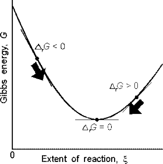
Figure 2. Ideal Gas Mixture: G vs. $\xi$

which implies that the Gibbs free energy is a convex function of the extent of reaction. An example of such a function is displayed in Fig.$2$, (see [22]), and defines the condition of stability. Initially, the Gibbs free energy decreases. As a reaction proceeds, the Gibbs free energy of the system continues to decrease until it reaches a minimum value. At equilibrium (constant T and p), the Gibbs energy is at the minimum, and $\Delta_{r}G$ is equal to zero. At greater extents of reaction the Gibbs free energy is greater than zero and increases.

This well-known result suggests for a non-ideal mixture the change in sign and vanishing of the second derivative of the Gibbs function might provide some insight into the stability of the system. In particular, consider the case in which the Gibbs free energy is not a simple convex function of the extent of the reaction everywhere, but rather, first convex, then concave, then convex again, as shown in Fig $3$. Points on the curve where changes between convex and concave behavior occur are inflection points which satisfy the expression in Eqn.$(3.18)$. Naturally, a shift of the equilibrium state from one local minimum to another constitutes a first order phase transition induced by a change in the extent of reaction [4]. For a chemical reaction, the system tends to approach chemical equilibrium where the forward and reverse reaction rates are the same and concentrations of the reactant and product species do not change with time. When the equilibrium condition is achieved, proportions of the various compounds remain unchanged, and the reaction ceases to progress. Prior to reaching the point of equilibrium, the system fluctuates between different equilibrium microstates. Suppose that the system is confined in a lower (more stable) Gibbs free-energy minimum and, occasionally, a fluctuation may be large enough to push the system over the maximum to the region of higher energy, i.e. a matastable minimum. A small fluctuation can overcome the shallow barrier back to the more stable equilibrium state [4]. Any thermodynamic system, in this case a chemical reaction, tends to eventually reach the lowest minimum in the Gibbs free energy. Naturally, if the ”unstable” barrier is too high or the minima are far apart a shift of the equilibrium from one local minimum state to another is less probable.

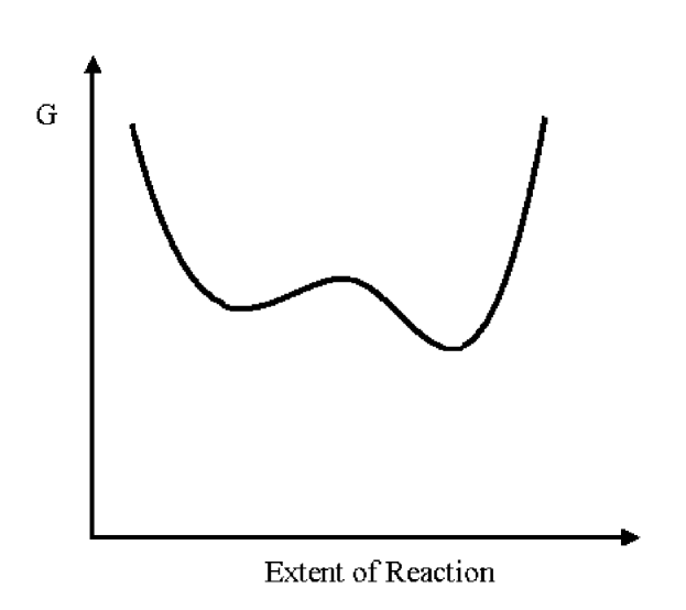
Figure 3. Non-ideal Mixture: G vs. $\xi$

Within this picture, the local curvature of the Gibbs free energy is positive for all points except those between the two inflection points. Moreover, the portion of the curve between the minima at the inflection points is said to be locally stable but globally unstable. In this region on the curve metastable states occur which appear to be stable to small perturbations, but mixed configurations at the same extent of reaction represent more stable states with lower free energy. A straight line connecting the two minima corresponds to a phase boundary [4], i.e. a phase transition from the phase at one minimum to the phase at the other minimum. Positive local curvature fails at the points of inflection. Local stability determines whether, after a small perturbation, a system will return to the original equilibrium state. Here our focus is on examining conditions leading to failure of local stability.

Remark 4.

Ideal Mixture. For an isothermal and isobaric ideal mixture,

$$\frac{d\Delta_{r}G}{d\xi}=\frac{RT}{\xi(1-\xi)}$$ (3.20)

When $T\neq{0}$, consider that

$$\frac{d\xi}{d\Delta_{r}G}=\frac{\xi(1-\xi)}{RT}=k\xi(1-\xi),\qquad k=\frac{1}{RT}>0$$ (3.21)

which is the so-called logistic equation [2]. The process described by this equation has two equilibrium positions, namely $\xi=0$ and $\xi=1$. Between these two points the field is directed from $0$ to $1$. As a result the equilibrium position $\xi=0$ is unstable (as soon as the reaction proceeds away from $\xi=0$ reactants are converted to products). Meanwhile the equilibrium position $\xi=1$ is stable. Moreover, integral curves tend asymptotically to the line $\xi=1$ as $\Delta_{r}G\rightarrow{+\infty}$ and to the line $\xi=0$ as $\Delta_{r}G\rightarrow{-\infty}$. Such curves describe the passage from one state (0) to another (1) in an infinite $\Delta_{r}G$.

3.2. Compounds

Consider a generic chemical reaction written as,

$$|\nu_{A}|A+|\nu_{B}|B+...\rightarrow{|\nu_{S}|S+|\nu_{T}|T+...}$$

where components on the left side are designated reactants while components on the right hand side are products [9]. The $|\nu_{i}|$, $i=A,B,...$ are stoichiometric coefficients of the reaction. Another formal representation of a chemical reaction which better lends itself to mathematical manipulation is given by [9],

$$\nu_{S}S+\nu_{T}T+...+\nu_{A}A+\nu_{B}B=\sum_{i}\nu_{i}i=0$$ (3.22)

The chemical potential of each component is given by [9],

$$\mu_{i}=\mu^{*}_{i}(T,p)+RT\ln{\gamma_{i}x_{i}}=\mu^{*}_{i}(T,p)+RT\ln{a_{i}}\qquad i=A,B,...$$ (3.23)

where $a_{i}$ is the activity of component $i$. Recall that $x_{i}=\frac{N_{i}}{\sum_{j}N_{j}}$, with $N_{i}=N^{0}_{i}+\nu_{i}\xi$ and that $\gamma_{i}$ depends on the extent of reaction. Thus, the Gibbs free-energy of the reaction is given by [9],

$$\Delta_{r}G=\sum_{i}\mu_{i}\nu_{i}=\sum_{i}\nu_{i}\mu^{*}_{i}+RT\ln{\prod_{i}a^{\nu_{i}}_{i}}=\sum_{i}\nu_{i}\mu^{*}_{i}+RT\ln{\prod_{i}\gamma^{\nu_{i}}_{i}x^{\nu_{i}}_{i}}$$ (3.24)

Introducing the quotient of reaction, $Q_{a}=\prod_{i}a^{\nu_{i}}_{i}=\prod_{i}\gamma^{\nu_{i}}_{i}\prod_{i}x^{\nu_{i}}_{i}=Q_{\gamma}Q_{c}$, where the subscript $c$ denotes concentration, the expression $(3.24)$ can be written as [9],

$$\Delta_{r}G=\Delta_{r}G^{\theta}+RT\ln{Q_{a}}$$ (3.25)

where $\Delta_{r}G^{\theta}=\sum_{i}\nu_{i}\mu^{*}_{i}(T,p^{\theta})$ is the standard Gibbs free energy of reaction. It follows that,

$$Q_{a}(\xi)=e^{\frac{\Delta_{r}G(\xi)-\Delta_{r}G^{\theta}}{RT}}$$ (3.26)

Naturally, if the system reaches equilibrium, namely $\Delta_{r}G=0$, the parameter $Q_{a}$ is denoted by $K_{a}$, the equilibrium constant, and the expression in $(3.26)$ becomes [9],

$$Q^{eq}_{a}=K_{a}=e^{-\frac{\Delta_{r}G^{\theta}}{RT}}$$ (3.27)

Thus, for an isothermal and isobaric single chemical reaction,

$$\frac{d\Delta_{r}G}{d\xi}=RT\frac{d{\ln{Q_{a}}}}{d{\xi}}=RT[\frac{d{\ln{Q_{c}}}}{d{\xi}}+\frac{d{\ln{Q_{\gamma}}}}{d{\xi}}]$$

$$=RT[\sum_{i}(\frac{\nu^{2}_{i}}{N_{i}})-\frac{(\sum_{i}\nu_{i})^{2}}{\sum_{i}N_{i}}+\frac{d}{d{\xi}}\ln{(\prod_{i}\gamma^{\nu_{i}}_{i})}]$$ (3.28)

where

$$\frac{d{\ln{Q_{c}}}}{d{\xi}}=\sum_{i}(\frac{\nu^{2}_{i}}{N_{i}})-\frac{(\sum_{i}\nu_{i})^{2}}{\sum_{i}N_{i}}$$ (3.29)

For simplicity, denote $\frac{d}{d{\xi}}\ln{(\prod_{i}\gamma^{\nu_{i}}_{i})}=W(\xi)$. Then, the expression in $(3.28)$ can be rewritten as,

$$\frac{d^{2}G}{d\xi^{2}}=RT[\sum_{i}(\frac{\nu^{2}_{i}}{N_{i}})-\frac{(\sum_{i}\nu_{i})^{2}}{\sum_{i}N_{i}}+W(\xi)]$$ (3.30)

The expression in $(3.29)$ denotes the influence of the relative amounts of reactants and products at each extent of the reaction while $W(\xi)$ represents the relative strength of non-ideal (inter-particle) interactions existent between products and reactants. Consequently, at any value of the extent of reaction, there is a ”possible” value of W such that the two mentioned forces exactly balance one another. Thus, at a given certain extent of the reaction determined by the relative amounts of reactants and products, $W$ at that point corresponds to the relative strength of non-ideal interactions that must exist between products and reactants for a failure of local stability.

Remark 5.

For the ideal gas mixture, $Q_{a}=Q_{c}=\frac{\xi}{1-\xi}$ and therefore, $\frac{dQ_{a}}{d\xi}=\frac{1}{(1-\xi)^{2}}>0$ (see Fig. $4$). In this case, $Q_{\gamma}=1$ and the expression in $(3.30)$ reduces to,

$$\frac{d^{2}G}{d\xi^{2}}=RT[\sum_{i}(\frac{\nu^{2}_{i}}{N_{i}})-\frac{(\sum_{i}\nu_{i})^{2}}{\sum_{i}N_{i}}]$$ (3.31)

Moreover, when the sum of the stoichiometric coefficients vanishes (i.e the isothermal-isobaric Ideal gas mixture, see $(3.19)$), the expression in $(3.30)$ reduces further to,

$$\frac{d^{2}G}{d\xi^{2}}=RT\sum_{i}(\frac{\nu^{2}_{i}}{N_{i}})>0$$ (3.32)

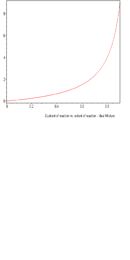
Figure 4. Ideal Mixture

Theorem 2.

Let $T\neq{0}$. Then, for an isobaric and isothermal single chemical reaction, $\frac{d^{2}G}{d\xi^{2}}=0$ if and only if

$$W(\xi)=\frac{(\sum_{i}\nu_{i})^{2}}{\sum_{i}N_{i}(\xi)}-\sum_{i}\frac{\nu^{2}_{i}}{N_{i}(\xi)}$$ (3.33)

The Gibbs free energy, $G$, is a convex function of the extent of reaction whenever,

$$W(\xi)>\frac{(\sum_{i}\nu_{i})^{2}}{\sum_{i}N_{i}(\xi)}-\sum_{i}\frac{\nu^{2}_{i}}{N_{i}(\xi)}$$ (3.34)

and a concave function whenever,

$$W(\xi)<\frac{(\sum_{i}\nu_{i})^{2}}{\sum_{i}N_{i}(\xi)}-\sum_{i}\frac{\nu^{2}_{i}}{N_{i}(\xi)}$$ (3.35)

The curve described by the expression in $(3.33)$ is denoted as the curve of phase boundary in the $W$-$\xi$ plane. Such a curve traces the phase boundary between the convex and concave regions of the Gibbs free energy. In particular, at a fixed value of the extent of reaction, the system is locally stable whenever the value of $W$ is less (in absolute value) than the value on the curve of phase boundary. If instead the value of $W$ is greater, the system is locally unstable.

In early stages of the reaction, reactant species are far in excess of product species, and $W$ is (in absolute value) relatively large. Since a change from reactant phase to product phase is improbable early in the reaction, interactions between products, favoring product formation, must be greater than those between reactants, favoring the reactant phase. $W$ indicates the balance of the strengths of the product and reactant interactions required for failure of local stability. As the reaction progresses toward the extremum of the curve of phase boundary, $\frac{dW}{d\xi}=0$, the relative difference in strength between the two types of interactions is a minimum. At this critical extent of reaction, a change between reactant and product phases requires the smallest difference between their constituent interactions and is thus most probable. Past this critical point the extent of reaction increases. To achieve local instability the relative strength of the interactions favoring reactants must be increasingly greater than those favoring the products.
Example II: Synthesis Reaction

Consider a simple synthesis reaction in which two or more substances combine to form a more complex substance. For example, $2$ moles of di-hydrogen react with $1$ mole of oxygen to give $2$ moles of water,

$$2H_{2}+O_{2}\rightarrow{2H_{2}O}$$ (3.36)

with

$$N_{H_{2}}=2-2\xi\qquad N_{O_{2}}=1-\xi\qquad and\qquad N_{H_{2}O}=2\xi$$

and the corresponding stoichiometric coefficients given by,

$$\nu_{H_{2}}=-2\qquad\nu_{O_{2}}=-1\qquad and\qquad\nu_{H_{2}O}=2$$

Then, from $(3.33)$,

$$W(\xi)=-\frac{6}{\xi(1-\xi)(3-\xi)}<0$$ (3.37)

A plot of the curve of phase boundary for this reaction is given in Fig.5.

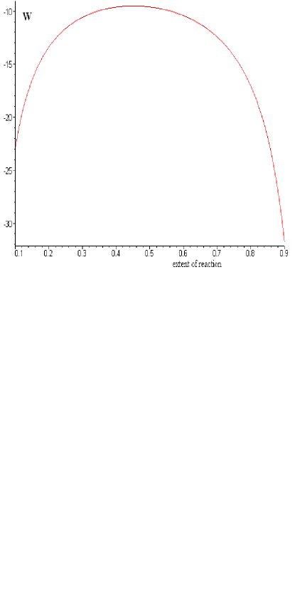
Figure 5. Synthesis Reaction: W vs. $\xi$

The extremum of this curve defines the ”most probable” transition point between the reactant and product phases. At this point differences in the relative amounts of reactant and product species, and relative differences in the strengths of their non-ideal interactions, are minimal. Taking the derivative with respect to $\xi$ (Fig.$6$) and setting it to zero yields,

$$\xi=0.4514$$

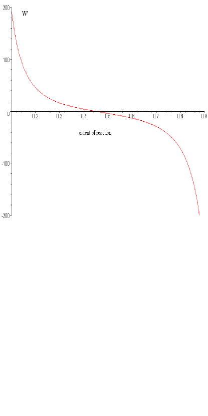
Figure 6. Synthesis Reaction: W’ vs. $\xi$

It follows that $W=-9.5$. The fact that the critical extent of the reaction is less than 0.5 suggests that the products and associated non-ideal interactions are more strongly favored such that the product phase is preferred even before half the extent of reaction is reached.

Now in analogy, consider the dissociation reaction, i.e. the synthesis reaction in the opposite direction. In this case $2$ moles of water split into $2$ moles of hydrogen and $1$ mole of oxygen. Namely,

$$2H_{2}O\rightarrow{2H_{2}+O_{2}}$$ (3.38)

Following the same steps as for analysis of the synthesis reaction, the following expression for $W$ is obtained,

$$W(\xi)=-\frac{6}{\xi(1-\xi)(2+\xi)}<0$$ (3.39)

The graph of this curve of phase boundary is shown in Fig.7.

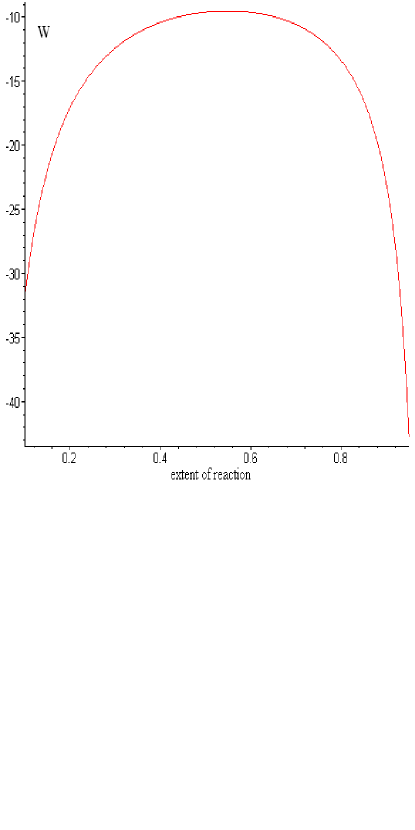
Figure 7. Dissociation Reaction: W vs. $\xi$

Taking the derivative with respect to $\xi$ and setting it to zero (see Fig.$8$),

$$\xi=0.5486$$

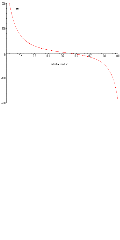
Figure 8. Dissociation Reaction: W’ vs. $\xi$

Note, $W=-9.5$ is apparently ”invariant” to the direction of the chemical reaction. The critical extent of reaction, $\xi$ = 0.5486 for the dissociation reaction, consistent with inferences drawn from analysis of the synthesis reaction. That is, interactions between the synthetic species ($H_{2}O$) are more favorable than those between the individual species ($H_{2}$, $O_{2}$). The sum of the two critical extents of reactions is $0.4514+0.5486=1$.
Example III: Single Displacement Reaction

A single displacement reaction is one in which an atom (or ion) of a single compound replaces an atom of another compound. As an example, consider the single displacement in which copper ions in a copper sulfate solution are displaced by zinc, forming zinc sulfate:

$$Zn+CuSO_{4}\rightarrow{Cu+ZnSO_{4}}$$ (3.40)

with,

$$N_{Zn}=1-\xi\qquad N_{CuSO_{4}}=1-\xi\qquad N_{Cu}=\xi\qquad and\qquad N_{ZnSO_{4}}=\xi$$

The corresponding stoichiometric coefficients are given by,

$$\nu_{Zn}=-1\qquad\nu_{CuSO_{4}}=-1\qquad\nu_{Cu}=1\qquad and\qquad\nu_{ZnSO_{4}}=1$$

Then, the expression in $(3.33)$ is given by,

$$W(\xi)=-\frac{2}{\xi(1-\xi)}<0$$ (3.41)

The graph of this curve of phase boundary for this reaction is shown in Fig.9.

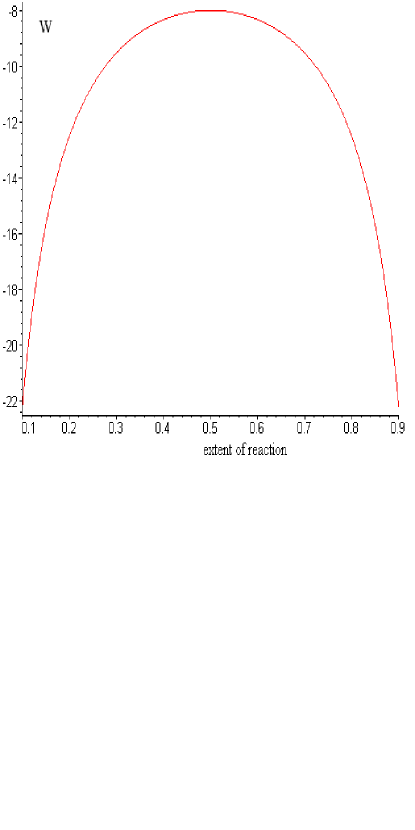
Figure 9. Single Displacement Reaction: W vs. $\xi$

Taking the derivative with respect to $\xi$ and setting it to zero (see Fig.$10$),

$$\xi=0.5$$

It follows that $W=-8$. In this case $\xi=0.5$ corresponds to the minimum difference between interactions associated with the product and reactant species for a phase transition to occur. Note that, for the displacement reaction, the critical extent of the reaction is $0.5$. In this case, the number of products species equals the number of reactants species and the critical extent of the reaction is independent of the direction of the process. This is in contrast to what was found for obtain in the synthesis and dissociation reactions where product and reactant species are not equal and the critical extent of the reaction depends on the reaction direction.

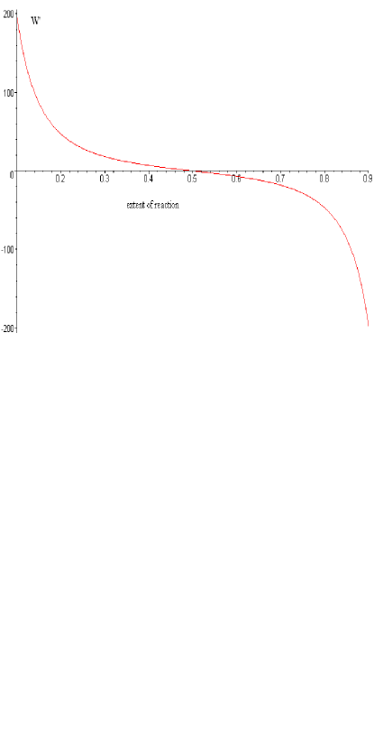
Figure 10. Single Displacement Reaction: W vs. $\xi$

3.3. Multi-chemical reaction

Here the Gibbs metric is introduced for a closed system with r chemical species in which $l$ independent reactions can occur. The total change of mass, $dm_{i}$, is equal to the sum of the changes resulting from the different reactions, [16],

$$dm_{i}=M_{i}\sum_{n}\nu_{in}d\xi_{n}\qquad n=1,..,l$$ (3.42)

The principle of Conservation of Mass can be stated as [16],

$$dm=\sum_{i}\sum_{n}\nu_{in}M_{i}d\xi_{n}=0$$ (3.43)

As done previously, consider the number of moles of the components in the system instead of their masses. The change in number of moles of component $i$ is given by,

$$dN_{i}=\sum_{n}\nu_{in}d\xi_{n}$$

The Legendre submanifold $\mathcal{S}_{G}$ is defined by the constitutive relation $G=G(T,p,\xi_{1},...\xi_{l})$ and the expression in Eqn.$(3.3)$ becomes,

$$\frac{dN_{1,n}}{\nu_{1,n}}=...=\frac{dN_{i,n}}{\nu_{i,n}}=...=d\xi_{n}$$

where $\xi_{n}$ is the extent of the n-th reaction with $i=1,...,r$ and $n=1,...,l$, [9]. Now, consider the differential of the Gibbs free-energy,

$$dG=-SdT+VdP-\sum_{n}A_{n}d\xi_{n}$$ (3.44)

By recalling the expression in $(1.16)$, the following metric is obtained,

$$\eta_{ij_{G}}=\begin{pmatrix}-\frac{C_{p}}{T}&{\alpha}V&-\Delta_{r}S_{1}&...&-\Delta_{r}S_{r}\\ {\alpha}V&-k_{T}V&\Delta_{r}V_{1}&...&\Delta_{r}V_{r}\\ -\Delta_{r}S_{1}&\Delta_{r}V_{1}&-(\frac{\partial{A_{1}}}{\partial{\xi_{1}}})_{T,p,\xi_{2},...\xi_{l}}&...&-(\frac{\partial{A_{l}}}{\partial{\xi_{1}}})_{T,p,\xi_{2},...\xi_{l}}\\ \vdots&\vdots&\vdots&...&\vdots\\ -\Delta_{r}S_{r}&\Delta_{r}V_{r}&-(\frac{\partial{A_{l}}}{\partial{\xi_{1}}})_{T,p,\xi_{2},...\xi_{l}}&...&-(\frac{\partial{A_{l}}}{\partial{\xi_{l}}})_{T,p,\xi_{1},...\xi_{l-1}}\end{pmatrix}$$ (3.45)

This is the Gibbs metric for a multicomponent thermodynamic system in which $l$ independent chemical reactions occur.

4. System 3: Open systems

Finally, consider open systems in the absence of external fields. Recall that the contact $1$-form $\theta$, restricted to the Legendre submanifold $\mathcal{S}_{G}$ described by the constitutive relation $G=G(T,p,N_{1},...,N_{r})$, gives the following differential, see $(1.39)$,

$$dG=-SdT+Vdp+\sum_{i}\mu_{i}dN_{i}$$ (4.1)

Define a partial molar quantity as [9],

$$\overline{X_{i}}=(\frac{\partial{X}}{\partial{N_{i}}})_{T,p,N_{j\neq{i}}}$$ (4.2)

Since the Gibbs metric is defined as the Hessian of the Gibbs potential, $\eta_{ij_{G}}=\frac{\partial^{2}{G}}{\partial{x^{i}}\partial{x^{j}}}$, where $x^{i}$ and $x^{j}$ are the extensive variables, the following result is obtained,

$$\eta_{ij_{G}}=\begin{pmatrix}-\frac{C_{p}}{T}&{\alpha}V&-\overline{S_{1}}&\cdots&-\overline{S_{r}}\\ {\alpha}V&-k_{T}V&\overline{V_{1}}&\cdots&\overline{V_{r}}\\ -\overline{S_{1}}&\overline{V_{1}}&\overline{\mu_{11}}&\cdots&\overline{\mu_{r1}}\\ \vdots&\vdots&\vdots&\cdots&\vdots\\ -\overline{S_{r}}&\overline{V_{r}}&\overline{\mu_{r1}}&\cdots&\overline{\mu_{rr}}\end{pmatrix}$$ (4.3)

where $\overline{\mu_{ik}}=(\frac{\partial{\mu_{i}}}{\partial{N_{k}}})_{T,p,N_{j\neq{k}}}$.

At constant temperature and pressure, conservation of energy $(4.1)$ reduces to,

$$dG=\sum_{i}\mu_{i}dN_{i}$$ (4.4)

Therefore, the metric in Eqn.$(4.3)$ becomes,

$$\eta_{ij_{G}}=\begin{pmatrix}\overline{\mu_{11}}&\overline{\mu_{21}}&\cdots&\overline{\mu_{r1}}\\ \overline{\mu_{21}}&\overline{\mu_{22}}&\cdots&\overline{\mu_{r2}}\\ \vdots&\vdots&\cdots&\vdots\\ \overline{\mu_{r1}}&\overline{\mu_{r2}}&\cdots&\overline{\mu_{rr}}\end{pmatrix}$$ (4.5)

4.1. Ideal solutions

Now, introduce the Gibbs metric for the cases of an ideal and non-ideal solution in an open thermodynamic system without chemical reactions. A component $i$ in solution is said to be ideal when its chemical potential is given by, [9],

$$\mu_{i}=\mu^{*}_{i}(T,p)+RT\ln{x_{i}}$$ (4.6)

where $\mu^{*}_{i}(T,p)$ is the standard state chemical potential which is independent of the composition and $x_{i}=\frac{N_{i}}{\sum_{j}N_{j}}=\frac{N_{i}}{N}$ is the mole fraction. Note, the total number of moles, N, depends on the number of moles of the r components, namely $N=N(N_{1},...,N_{r})$.

Using the expression $(4.6)$, the metric for an ideal solution that depends on the temperature and the pressure of the system is obtained,

$$\eta_{ij_{G}}=\begin{pmatrix}-\frac{C_{p}}{T}&{\alpha}V&(\frac{\partial{\mu^{*}_{1}}}{\partial{T}})_{p,N_{i}}+R\ln{x_{1}}&\cdots&(\frac{\partial{\mu^{*}_{r}}}{\partial{T}})_{p,N_{i}}+R\ln{x_{r}}\\ {\alpha}V&-k_{T}V&(\frac{\partial{\mu^{*}_{1}}}{\partial{p}})_{T,N_{i}}&\cdots&(\frac{\partial{\mu^{*}_{r}}}{\partial{p}})_{T,N_{i}}\\ (\frac{\partial{\mu^{*}_{1}}}{\partial{T}})_{p,N_{i}}+R\ln{x_{1}}&(\frac{\partial{\mu^{*}_{1}}}{\partial{p}})_{T,N_{i}}&RT(\frac{1}{N_{1}}-\frac{1}{N})&\cdots&-\frac{RT}{N}\\ \vdots&\vdots&\vdots&\cdots&\vdots\\ (\frac{\partial{\mu^{*}_{r}}}{\partial{T}})_{p,N_{i}}+R\ln{x_{r}}&(\frac{\partial{\mu^{*}_{r}}}{\partial{p}})_{T,N_{i}}&-\frac{RT}{N}&\cdots&RT(\frac{1}{N_{r}}-\frac{1}{N})\end{pmatrix}$$ (4.7)

For an isothermal-isobaric system such a metric becomes,

$$\eta_{ij_{G}}=\begin{pmatrix}RT(\frac{1}{N_{1}}-\frac{1}{N})&-\frac{RT}{N}&\cdots&-\frac{RT}{N}\\ -\frac{RT}{N}&RT(\frac{1}{N_{2}}-\frac{1}{N})&\cdots&-\frac{RT}{N}\\ \vdots&\vdots&\cdots&\vdots\\ -\frac{RT}{N}&-\frac{RT}{N}&\cdots&RT(\frac{1}{N_{r}}-\frac{1}{N})\end{pmatrix}$$ (4.8)

This metric is degenerate everywhere since $\det(\eta_{ij_{G}})=0$ for all values of the number of moles of the r components. This result indicates the Gibbs free energy metric for an open system does not distinguish differences between ideal components. As far as the metric is concerned, due to the explicit lack of inter-component interactions, the system is apparently comprised of a single, indistinguishable, ideal component.

4.2. Non-Ideal solutions

For non-ideal systems, the chemical potential of component $i$ takes the form, [9],

$$\mu_{i}=\mu^{*}_{i}(T,p)+RT\ln{\gamma_{i}x_{i}}$$ (4.9)

where $\gamma_{i}$ is the activity coefficient of species $i$ that depends on temperature, pressure and composition of the solution. Expression $(4.9)$ considers deviations from ideality. The partial molar entropy, $\overline{S_{i}}$, and the partial molar volume of component $i$, $\overline{V_{i}}$, are given by,

$$-\overline{S_{i}}=(\frac{\partial{\mu^{*}_{i}}}{\partial{T}})_{p,N_{i}}+R[\ln{\gamma_{i}x_{i}}+T(\frac{\partial{\ln{\gamma_{i}}}}{\partial{T}})_{p,N_{i}}]$$ (4.10)

and

$$\overline{V_{i}}=(\frac{\partial{\mu^{*}_{i}}}{\partial{p}})_{T,N_{i}}+RT(\frac{\partial{\ln{\gamma_{i}}}}{\partial{p}})_{T,N_{i}}$$ (4.11)

Moreover,

$$\overline{\mu_{ii}}=(\frac{\partial{\mu_{i}}}{\partial{N_{i}}})_{T,p,N_{j\neq{i}}}=RT[(\frac{1}{N_{i}}-\frac{1}{N})+(\frac{\partial{\ln{\gamma_{i}}}}{\partial{N_{i}}})_{T,p,N_{j\neq{i}}}]$$ (4.12)

and,

$$\overline{\mu_{ik}}=(\frac{\partial{\mu_{i}}}{\partial{N_{k}}})_{T,p,N_{j\neq{k}}}=RT[-\frac{1}{N}+(\frac{\partial{\ln{\gamma_{i}}}}{\partial{N_{k}}})_{T,p,N_{j\neq{k}}}]$$ (4.13)

For symplicity, denote $(\frac{\partial{\ln{\gamma_{i}}}}{\partial{N_{k}}})_{T,p,N_{j\neq{k}}}=\overline{(\ln{\gamma_{i}})}_{k}$ and retain the usual notation for partial molar entropy and volume. Substituting the expressions $(4.10)$-$(4.13)$ into the metric $(4.3)$, the general metric of a multicomponent non-ideal solution is obtained,

$$\eta_{ij_{G}}=\begin{pmatrix}-\frac{C_{p}}{T}&{\alpha}V&-\overline{S_{1}}&\cdots&-\overline{S_{r}}\\ {\alpha}V&-k_{T}V&\overline{V_{1}}&\cdots&\overline{V_{r}}\\ -\overline{S_{1}}&\overline{V_{1}}&RT[(\frac{1}{N_{1}}-\frac{1}{N})+\overline{(\ln{\gamma_{1}})}_{1}]&\cdots&RT[-\frac{1}{N}+\overline{(\ln{\gamma_{r}})}_{1}]\\ \vdots&\vdots&\vdots&\cdots&\vdots\\ -\overline{S_{r}}&\overline{V_{r}}&RT[-\frac{1}{N}+\overline{(\ln{\gamma_{r}})}_{1}]&\cdots&RT[(\frac{1}{N_{r}}-\frac{1}{N})+\overline{(\ln{\gamma_{r}})}_{r}]\end{pmatrix}$$ (4.14)

and, in the case of an isobaric-isothermal non-ideal system, the Gibbs metric simplifies to,

$$\eta_{ij_{G}}=RT\begin{pmatrix}[(\frac{1}{N_{1}}-\frac{1}{N})+\overline{(\ln{\gamma_{1}})}_{1}]&[-\frac{1}{N}+\overline{(\ln{\gamma_{2}})}_{1}]&\cdots&[-\frac{1}{N}+\overline{(\ln{\gamma_{r}})}_{1}]\\ [-\frac{1}{N}+\overline{(\ln{\gamma_{2}})}_{1}]&[(\frac{1}{N_{2}}-\frac{1}{N})+\overline{(\ln{\gamma_{2}})}_{2}]&\cdots&[-\frac{1}{N}+\overline{(\ln{\gamma_{r}})}_{2}]\\ \vdots&\vdots&\vdots&\vdots\\ [-\frac{1}{N}+\overline{(\ln{\gamma_{r}})}_{1}]&[-\frac{1}{N}+\overline{(\ln{\gamma_{r}})}_{2}]&\cdots&[(\frac{1}{N_{r}}-\frac{1}{N})+\overline{(\ln{\gamma_{r}})}_{r}]\end{pmatrix}$$ (4.15)

$$=RT[\begin{pmatrix}(\frac{1}{N_{1}}-\frac{1}{N})&-\frac{1}{N}&\cdots&-\frac{1}{N}\\ -\frac{1}{N}&(\frac{1}{N_{2}}-\frac{1}{N})&\cdots&-\frac{1}{N}\\ \vdots&\vdots&\cdots&\vdots\\ -\frac{1}{N}&-\frac{1}{N}&\cdots&(\frac{1}{N_{r}}-\frac{1}{N})\end{pmatrix}+\begin{pmatrix}\overline{(\ln{\gamma_{1}})}_{1}&\overline{(\ln{\gamma_{2}})}_{1}&\cdots&\overline{(\ln{\gamma_{r}})}_{1}\\ \overline{(\ln{\gamma_{2}})}_{1}&\overline{(\ln{\gamma_{2}})}_{2}&\cdots&\overline{(\ln{\gamma_{r}})}_{2}\\ \vdots&\vdots&\cdots&\vdots\\ \overline{(\ln{\gamma_{r}})}_{1}&\overline{(\ln{\gamma_{r}})}_{2}&\cdots&\overline{(\ln{\gamma_{r}})}_{r}\end{pmatrix}]$$ (4.16)

$$=(\eta_{ij_{G}})_{ideal}+(\eta_{ij_{G}})_{deviation}$$ (4.17)

where the subscript ”deviation” indicates the degree of non-ideality.

5. Conclusions

Geometrical thermodynamics has been applied to study the behavior of several simple thermodynamic systems. For a single component, closed system intriguing relationships between the geometrical concepts of degeneracy and scalar curvature of the Weinhold metric, and the physical concepts of a phase transition and inter-particle, non-ideal interactions are divulged. For multi-component closed systems the Gibbs metric was presented and the scalar curvature and degeneracy of this metric was determined for a few simple cases and could be indicative of physical behavior. In summary, this study provides convincing examples that this geometrical approach to analysis of thermodynamic systems can be applied to actually divulge important physical and chemical behavior.

References

- [1] V. Arnold, Mathematical Methods of Classical Mechanics, Springer Verlag.
- [2] V. Arnold, Ordinary Differential Equations, Springer Verlag.
- [3] J. Boyling, Caratheodory’s Principle and the Existence of Global Integrating Factors, Commun.Math.Phys., 10, pp.52-68, 1968.
- [4] H.B. Callen, Thermodynamics, Whiley, 1960.
- [5] A. Cannas da Silva, Lectures on Symplectic Geometry, Lecture Notes in Mathematics, Springer, 2000.
- [6] C. Caratheodory, Unterschungen uber die Grundlagen der T, hermodynamyk, Mathematishe Annalen, 67, pp.355-386, 1909.
- [7] C. Caratheodory, Unterschungen uber die Grundlagen der Thermodynamyk, Gesammelte Mathematische Werke, B.2., Munchen, pp.131-177, 1955.
- [8] J. Gibbs, The Collected Works, v.1, Thermodynamics, Yale Univ. Press, 1948.
- [9] M. Graetzel, P. Infelta, The Bases of Chemical Thermodynamics, Vol. I,II, Universal Publishers.
- [10] R. Hermann, Geometry, Physics and Systems, Dekker, N.Y., 1973.
- [11] R. Mrugala, Geometrical Formulation of Equilibrium Phenomenological Thermodynamics,Reports of Mathematical Physics, v.14,No.3, pp.419-427, 1978.
- [12] R. Mrugala, On equivalence of two metrics in classical thermodynamics, Physica A,v.125, pp.631-639, 1984.
- [13] R. Mrugala, J.D. Nulton, J.C. Schoen, P. Salamon, Contact structure in thermodynamic theory, Reports of Mathematical Physics, v.29, No.1, pp.109-121, 1991.
- [14] R. Mrugala, On a Riemannian Metric on Contact Thermodynamic Spaces, Reports of Mathematical Physics, v.38, No.3, pp.339-348, 1996.
- [15] S.Preston, Notes on the geometrical structures of homogeneous thermodynamics, manuscript, 2004.
- [16] I. Prigogine, Thermodynamics of Irreversible Processes, Interscience Publishers, 1968.
- [17] G.Ruppeiner, Thermodynamics:A Riemannian geometric model, Phys. Review A. 20(4), pp.1608-1613, 1979.
- [18] G. Ruppeiner,Riemannian geometry approach to critical points: General theory, Phys. Review E, v.57,n.5, pp.5135-5145, 1998.
- [19] P.Salamon, J.Nulton, E. Ihrig,On the relation between entropy and energy versions of thermodynamic length J.Chem. Phys., 80, 436, 1984.
- [20] M. Santoro, S. Preston, Curvature of the Weinhold Metric for Thermodynamical Systems with 2 degrees of freedom, arXiv,org, math-ph/0505010, May 2005.
- [21] F. Weinhold, Metric Geometry of equilibrium thermodynamics,p. I-V,Journal of Chemical Physics, v.63, n.6,2479-2483, 2484-2487, 2488-2495,2496-2501,1976, v.65,n.2,pp.559-564,1976.
- [22] Fig. has been taken from ”http://www2.mcdaniel.edu/Chemistry/ch307.notes/ Chemical20Equilibrium.html”.