Further properties of causal relationship: causal structure stability, new criteria for isocausality and counterexamples

Abstract

Recently (Class. Quant. Grav. 20 625-664) the concept of causal mapping between spacetimes –essentially equivalent in this context to the chronological map one in abstract chronological spaces–, and the related notion of causal structure, have been introduced as new tools to study causality in Lorentzian geometry. In the present paper, these tools are further developed in several directions such as: (i) causal mappings –and, thus, abstract chronological ones– do not preserve two levels of the standard hierarchy of causality conditions (however, they preserve the remaining levels as shown in the above reference), (ii) even though global hyperbolicity is a stable property (in the set of all time-oriented Lorentzian metrics on a fixed manifold), the causal structure of a globally hyperbolic spacetime can be unstable against perturbations; in fact, we show that the causal structures of Minkowski and Einstein static spacetimes remain stable, whereas that of de Sitter becomes unstable, (iii) general criteria allow us to discriminate different causal structures in some general spacetimes (e.g. globally hyperbolic, stationary standard); in particular, there are infinitely many different globally hyperbolic causal structures (and thus, different conformal ones) on $\mathbb{R}^{2}$, (iv) plane waves with the same number of positive eigenvalues in the frequency matrix share the same causal structure and, thus, they have equal causal extensions and causal boundaries.

and

1 Introduction

Lorentzian (time-oriented) manifolds are naturally equipped with a notion of causal structure. Traditionally this has been related to two concepts: (A) the classical causality theory, based on the binary relations “$\leq$” (causality) and “$\ll$” (chronology) from which one defines the basic sets $I^{+}(p),I^{-}(p),J^{+}(p),J^{-}(p)$, and (B) the conformal structure generated by the Lorentzian metric. Even though all these approaches are well settled, the elements present in (A) and (B) have specific characteristics, and it is not clear if they must be regarded as the unique ingredients in a sensible definition of causal structure. As an extreme example, in any totally vicious spacetime all the points are related by “$\ll$”; but there are many different types of totally vicious spacetimes, and it is not evident why all of them should be deemed as bearing the same causal structure. On the other hand, the conformal structure is very restrictive and, frequently, it seems reasonable to consider some non–conformally related spacetimes as causally equivalent (otherwise, the concept of causality itself would mean just conformal structure in Lorentzian signature, and would be rather redundant). For example, most modifications of a Lorentzian metric around a point (say, any non-conformally flat perturbation of Minkowski spacetime in a small neighbourhood) imply a different conformal structure; but, one may have a very similar structure of future and past sets for all points.

Two points $p$, $q$ of a Lorentzian manifold are related by “$\ll$” (resp. “$\leq$”) if they can be joined by a future-directed timelike (resp causal) curve. Hence classical causality (a global concept) stems from the Lorentzian cone (a local concept) but the passage from the latter to the former is not fully grasped by the connectivity properties of the above binary relations as we hope to make clear in this paper with examples. Nevertheless, recall that, in any distinguishing spacetime, the (too restrictive) conformal structure is determined by the (too general) binary causal relations induced locally by the metric. Thus, to find a concept which retains the essentials of binary causal relations but not reducible (in causally well-behaved spacetimes) to the conformal structure, becomes a subtle question. This concept should lie somewhere in between the local information provided by the light cones and the global character of the binary causal relations.

In [14] a new viewpoint toward this issue was put forward. The idea is to define mappings between Lorentzian manifolds which transform causal vectors into causal vectors or causal mappings, and so they preserve the relations “$\ll$” and “$\leq$”. Their possible existence between two spacetimes induces a concept of causal equivalence or isocausality as well as a partial ordering on the set of all the Lorentzian manifolds. As causal mappings are more flexible than conformal ones, they are a new invaluable tool to address in precise terms what is meant by “the causal structure” of the spacetime (see sections 4.2 and 4.3 of [15] for a summary).

The present paper makes a deeper study of such mappings and the associated causal relationships, extending and improving [14] in several directions: (i) to consolidate the foundations of the theory, settling, for example, unsolved issues on the relation between causal mappings and causal hierarchy, (ii) to discuss new related ingredients, as the stability of the causal structure, (iii) to obtain criteria (such as obstructions to the existence of causal mappings) which make the theory more applicable, and (iv) to apply them in some relevant families of spacetimes, which include globally hyperbolic ones and pp-waves.

This paper is organised as follows: in section 2, firstly, the essential properties of causal mappings proven in [14] are briefly summarized and revisited. Some clarifying properties and examples are provided, such as example 2.1 on the role of time-orientation, example 2.2 on totally ordered chains by causal mappings, or proposition 2.6, which deals with the stability of the existence of a causal mapping. Also we put forward the notion of causal embedding boundary in subsection 2.3. Remarkably, in the last subsection the stability of the causal structure of Minkowski spacetime $\mathbb{L}^{n}$ is proven by finding a generic family of isocausal perturbations of the metric (theorem 2.2). The aim of this result is twofold: on one hand, it shows the (desirable) stability of the causal structure of $\mathbb{L}^{n}$; on the other hand, as these perturbed metrics are generically non-conformally flat, this supports the claim that the causal structure is induced from causal mappings and, thus, it is a more general structure than the conformal one.

In section 3, first we connect causal mappings with more abstract approaches such as Harris “chronological mappings” (which preserve “$\ll$”, see [18]), and we show that, even though the former are more restrictive than the latter, they become equivalent in causally well-behaved spacetimes, theorem 3.1. Then, we study at what extent the standard hierarchy of causality conditions is preserved by causal mappings. Despite being known that most of the conditions of this hierarchy are preserved ([14, theorem 5.1], see theorem 2.1 below), the preservation of two levels –causally simple and causally continuous– remained open. We give an explicit counterexample answering the question in the negative. We emphasize that this counterexample also works for related concepts such as chronological mappings, and the implications thereof are discussed.

In section 4, new obstructions to the existence of causal mappings between two spacetimes are provided. These obstructions have a different nature to those presented in [14] where all are rooted in the causal hierarchy and in proposition 2.3 below. So, our new criteria show the nonexistence of causal mappings between spacetimes belonging to the same level of the standard hierarchy (example 4.2), allowing us to find many different causal structures, even in spaces as simple as rectangles (example 4.1) or globally hyperbolic open subsets of $\mathbb{L}^{2}$ (example 4.3). In particular, results about the existence of infinitely many different simply-connected conformal Lorentz surfaces by Weinstein [43] are extended.

In the last two sections, a first causal classification of two relevant families of spacetimes is carried out. Concretely, in section 5 a general family of smooth products $I\times S,I\subseteq\mathbb{R}$, which includes both, standard stationary and globally hyperbolic spacetimes, is studied. Time arrival functions $T^{\pm}$ (introduced in [34, 32]) are shown to be related to the existence of particle horizons and, then, to obstructions to the existence of causal mappings. Among the many results of this section, we highlight the following three: (1) a general criterion on the existence of causal mappings applicable to globally hyperbolic spacetimes (theorem 5.1), (2) a classification of the causal structures of spatially closed generalized Robertson Walker (GRW) spacetimes, (theorem 5.2), and (3) the instability of the causal structure of de Sitter spacetime (theorem 5.3), in clear difference with the stability of its global hyperbolicity, or the stability of $\mathbb{L}^{n}$ or other GRW spacetimes, as Einstein static Universe.

In section 6 we consider a general family of metrics including the important case of $pp$-waves and we give a general criterion for the existence of causal mappings, theorem 6.1. Then, we focus on plane waves, and among other results, we prove that locally symmetric plane waves are isocausal whenever their frequency matrices have the same signature, proposition 6.1. In the last subsection, we explain how this approach yields information about causal boundaries of plane waves according to the notion introduced in subsection 2.3. In particular, we prove that in the case of the frequency matrix being negative definite the plane wave admits a causal extension to $\mathbb{L}^{n}$ and a causal embedding boundary consisting of two lightlike planes. This holds even if the spacetime is not conformally flat, a case never tackled before as far as we know.

2 Essentials of causal relationship

2.1 Basic framework

In next paragraphs we recall basic concepts of [14] which will be profusely used in this work. Italic capital letters $V,W,$ … will denote differentiable $C^{\infty}$ manifolds and eventually we will use subscripts $V_{1}$, $V_{2}$ or a tilde, $\tilde{V}$. Boldface letters will be reserved for elements of the tensor bundle associated to a manifold (we use this same convention to represent sections of this bundle leaving to the context the distinction between each case). The special case of vectors and vector fields will be distinguished by adding an arrow to the boldface symbol. $(V,{\bf g})$ will denote a time-oriented Lorentzian manifold with metric tensor ${\bf g}$ (eventually with subscripts, if there is more than one) but we will sometimes abuse of the notation and use only the capital symbol to denote the Lorentzian manifold. We choose the signature convention $(+,-,\dots,-)$ which means that a vector $\vec{\boldsymbol{u}}$ is timelike if ${\bf g}(\vec{\boldsymbol{u}},\vec{\boldsymbol{u}})>0$, lightlike if ${\bf g}(\vec{\boldsymbol{u}},\vec{\boldsymbol{u}})=0$ and spacelike otherwise. Timelike and lightlike vectors are called causal vectors and the causal vector $\vec{\boldsymbol{u}}$ is future-directed if ${\bf g}(\vec{\boldsymbol{u}},\vec{\boldsymbol{v}})>0$ where $\vec{\boldsymbol{v}}\neq\vec{\boldsymbol{u}}$ is the causal vector defining the causal orientation. As usual, we denote $I^{+}(p)=\{x\in V:p\ll x\},\ J^{+}(p)=\{x\in V:p\leq x\}$, and analogously for their past duals. Smooth maps between manifolds are represented by Greek letters and if $\Phi:V_{1}\rightarrow V_{2}$ is any of such maps then the push-forward and pull-back constructed from it are $\Phi_{*}\boldsymbol{T}$ and $\Phi^{*}\boldsymbol{T}$ respectively.

Definition 2.1.

Let $\Phi:V_{1}\rightarrow V_{2}$ be a global diffeomorphism between two manifolds. We say that the Lorentzian manifold $V_{2}$ is causally related to $V_{1}$ by $\Phi$, denoted $V_{1}\prec_{\Phi}V_{2}$, if for every causal future-directed $\vec{\boldsymbol{u}}\in T(V_{1})$, $\Phi_{*}\vec{\boldsymbol{u}}\in T(V_{2})$ is causal future directed too. The diffeomorphism $\Phi$ is then called a causal mapping. $V_{2}$ is said to be causally related to $V_{1}$, denoted simply by $V_{1}\prec V_{2}$, if there exists a causal mapping $\Phi$ such that $V_{1}\prec_{\Phi}V_{2}$.

Remark 2.1.

The diffeomorphism $\Phi$ is a causal mapping if and only if the lightcones of the pull-back metric $\Phi^{*}{\bf g}_{2}$ include the cones of ${\bf g}_{1}$, and the time-orientations are preserved. Thus, for practical purposes, one can consider a single differentiable manifold $V$ in which two Lorentzian metrics ${\bf g}_{1}$, ${\bf g}_{2}$ are defined and wonder when the cones of ${\bf g}_{2}$ are wider than the cones of ${\bf g}_{1}$ (i.e., the identity in $V$ is a causal mapping). Some of the forthcoming results are formulated in this picture. In our exposition we will resort to one or other picture depending on what we wish to emphasize in each context.

A similar definition in which causal past-directed vectors are mapped into causal future-directed ones (anticausal mapping) can also be given. All the results described below hold likewise for causal and anticausal mappings although we only make them explicit for causal mappings. Nevertheless, the existence of a causal mapping does not imply the existence of a anti-causal one, nor vice versa (example 2.1 below). Causal and anticausal mappings are then characterized by the condition

$${\bf g}_{2}(\Phi_{*}\vec{\boldsymbol{u}},\Phi_{*}\vec{\boldsymbol{u}})=\Phi^{*}{\bf g}_{2}(\vec{\boldsymbol{u}},\vec{\boldsymbol{u}})\geq 0,\ \ \ \forall\,\vec{\boldsymbol{u}},\in T(V_{1})\ \mbox{causal future-directed}.$$ (2.1)

This means that $\Phi^{*}{\bf g}_{2}$ satisfies the weak energy condition which is a well-known algebraic condition in General Relativity for the stress energy tensor, but also applicable to any symmetric rank-2 covariant tensor. Alternatively, we find that $\Phi$ is causal or anticausal iff

$${\bf g}_{2}(\Phi_{*}\vec{\boldsymbol{u}}_{1},\Phi_{*}\vec{\boldsymbol{u}}_{2})=\Phi^{*}{\bf g}_{2}(\vec{\boldsymbol{u}}_{1},\vec{\boldsymbol{u}}_{2})\geq 0,\ \ \ \forall\,\vec{\boldsymbol{u}}_{1},\ \vec{\boldsymbol{u}}_{2}\in T(V_{1})\ \mbox{causal future-directed},$$ (2.2)

which means that $\Phi^{*}{\bf g}_{2}$ satisfies the dominant property another of the standard energy conditions used in General Relativity. For a general rank 2 symmetric tensor, this condition is more restrictive than the weak energy condition but, as $\Phi^{*}{\bf g}_{2}$ is a Lorentzian scalar product at each point, both conditions become equivalent here (see remark 2.2 for further details).

Clearly the relation “$\prec$” is a preorder in the set of all the diffeomorphic Lorentzian manifolds. Other basic properties easy to prove are the following [14].

Proposition 2.1 (Basic properties of causal mappings).

If $V_{1}\prec_{\Phi}V_{2}$, then:

1. All timelike future-directed vectors on $V_{1}$ are mapped to timelike future-directed vectors. If the image $\Phi_{*}\vec{\boldsymbol{u}}$ of a causal vector $\vec{\boldsymbol{u}}$ is future-directed lightlike, then $\vec{\boldsymbol{u}}$ is a future-directed lightlike vector.

2. Every future-directed timelike (causal) curve is mapped by $\Phi$ to a future-directed timelike (causal) curve (this property characterizes causal mappings; the timelike curves can be regarded smooth or only continuous in a natural sense).

3. For every set $S_{1}\subseteq V_{1}$, $\Phi(I^{\pm}(S_{1}))\subseteq I^{\pm}(\Phi(S_{1}))$, $\Phi(J^{\pm}(S_{1}))\subseteq J^{\pm}(\Phi(S_{1}))$, and $D^{\pm}(\Phi(S_{1}))\subseteq\Phi(D^{\pm}(S_{1}))$.

4. If a set $S_{2}\subset V_{2}$ is acausal (achronal), then $\Phi^{-1}(S_{2})$ is acausal (achronal).

5. If $S_{2}\subset V_{2}$ is a Cauchy hypersurface, then $\Phi^{-1}(S_{2})$ is a Cauchy hypersurface in $V_{1}$.

6. $\Phi^{-1}(F)$ is a future set for every future set $F\subset V_{2}$; and $\Phi^{-1}(\partial F)$ is an achronal boundary for every achronal boundary $\partial F\subset V_{2}$.

The inverse of a causal mapping is not necessarily a causal mapping, in fact:

Proposition 2.2.

For a diffeomorphism $\Phi:(V_{1},{\bf g}_{1})\rightarrow(V_{2},{\bf g}_{2})$ the following assertions are equivalent:

1. $\Phi$ (and, thus, $\Phi^{-1}$) is conformal, i.e., $\Phi^{*}{\bf g}_{2}=\lambda{\bf g}_{1}$, for some function $\lambda>0$.

2. $\Phi$ and $\Phi^{-1}$ are both causal or both anticausal mappings.

Of course, one can find pairs of Lorentzian manifolds $V_{1}$, $V_{2}$ such that $V_{1}\prec V_{2}$ but $V_{2}\not\prec V_{1}$ (this last statement means that there is no diffeomorphism $\Phi:V_{2}\rightarrow V_{1}$ which is a causal mapping). Given two diffeomorphic Lorentzian manifolds $V_{1}$, $V_{2}$ whether $V_{1}\prec V_{2}$ or $V_{1}\not\prec V_{2}$ cannot in principle be solved in simple terms. In some relevant examples, the relation $V_{1}\prec V_{2}$ can be proved by constructing explicitly a causal mapping, but specific techniques are needed to prove $V_{1}\not\prec V_{2}$. This was partly tackled in [14], where explicit examples in which causal mappings could not be constructed were provided. In all of them, there is a global causal property or condition not shared by the spacetimes, which forbids the existence of the causal mapping in at least one direction. These criteria are essentially contained in the following two results.

Theorem 2.1.

If $V_{1}\prec V_{2}$ and $V_{2}$ is globally hyperbolic, causally stable, strongly causal, distinguishing, causal, chronological, or not totally vicious, then so is $V_{1}$.

The conditions appearing in this last result comprise most of the so-called standard hierarchy of causality conditions. They have been extensively studied in the literature; so, one may check by independent methods if these conditions are fulfilled. Even more, one can check that the whole scale of “virtuosity” between strongly and stably causal spacetimes introduced by Carter [10], is also preserved in the sense that if $V_{2}$ is virtuous to the $n$th-degree so is $V_{1}$ (an brief account of Carter’s classification can be found in [15]). Thus, according to theorem 2.1 if $V_{2}$ meets one of these conditions of the hierarchy but $V_{1}$ does not, we deduce that $V_{1}\not\prec V_{2}$.

Proposition 2.3.

Suppose that there is an inextendible causal curve $\gamma\in V_{1}$ such that $I^{+}(\gamma)=V_{1}$ (resp. $I^{-}(\gamma)=V_{1}$) but no such curve exists in $V_{2}$. Then $V_{1}\not\prec V_{2}$.

The assumptions in proposition 2.3 imply that any inextendible causal curve in $V_{2}$ has a particle horizon (future particle horizon if $I^{+}(\gamma)\neq V_{2}$, past particle horizon otherwise). The presence of particle horizons for any inextendible causal curve is known in simple Lorentzian manifolds. Perhaps the most famous example in which this property holds is de Sitter spacetime where any inextendible causal curve has both future and past particle horizons. In this case proposition 2.3 implies that there is no causal mapping from Einstein static universe to de Sitter spacetime, although a causal mapping in the opposite way does exist ([14, example 2]; this will be widely extended in corollaries 5.1, 5.3). We give now another straightforward application, in order to show the role of the time-orientation.

Example 2.1.

Consider the spacetime $V$ depicted in figure 1. Any inextendible causal curve $\gamma$ in this spacetime has a future particle horizon. Nevertheless, the timelike curve represented by the $t$-axis does not have a past particle horizon. If the time orientation is reversed, the roles of the future and past horizons are interchanged and, thus, there is no causal mapping from the original spacetime to the spacetime with the reversed time-orientation, and vice versa. This example is analogous to a flat Friedman-Robertson-Walker spacetime with no pressure.

Figure 1: Example of a two-dimensional spacetime with inequivalent causal orientations (in this and in the remaining pictures we colour in black the past sheet of the causal cone). With this causal orientation any (inextendible) causal curve $\gamma$ has a future particle horizon (this is the line $x=1$ if the curve lies in the region $x<1$ or $x=-1$ if the curve lies in the region $x>-1$) but no timelike curve has a past particle horizon. The spacetime is invariant under translations of the $t$ coordinate.

2.2 Causal structures

We have seen that $V_{1}\prec V_{2}$ can be true despite the spacetimes $V_{1}$, $V_{2}$ having rather different causal properties (for instance $V_{1}$ can be globally hyperbolic and $V_{2}$ totally vicious). Things are drastically different if $V_{1}\prec V_{2}$ and $V_{2}\prec V_{1}$, so one defines:

Definition 2.2.

Two Lorentzian manifolds $V_{1}$ and $V_{2}$ are called causally equivalent or isocausal if $V_{1}\prec V_{2}$ and $V_{2}\prec V_{1}$. The relation of causal equivalence is denoted by $V_{1}\sim V_{2}$.

Traditionally two Lorentzian manifolds have been regarded as “causally equivalent” when they are conformally related. In principle, this was a sensible point of view because conformal transformations put the light cones into a bijective correspondence. However, the existence of a conformal relation is a too restrictive assumption because, as shown in [14], there are many examples (isolated bodies, exterior of black hole regions, etc.) in which one may speak of “essentially equal global causal properties” or “equivalent causality” but no conformal relation exists. These examples are isocausal in the above sense. Interestingly enough any pair of Lorentzian manifolds $V_{1}$, $V_{2}$ are locally causally equivalent, this meaning that one can choose neighbourhoods of the points $p_{1}\in V_{1}$, $p_{2}\in V_{2}$ which are causally equivalent when regarded as Lorentzian submanifolds (see theorem 4.4 of [15]).

If $V_{1}\sim V_{2}$ and one of the Lorentzian manifolds complies with the causality conditions stated in the theorem 2.1, then so does the other. Therefore the relation “$\sim$” maintains these causality conditions (see subsection 3.2 for the causality conditions not included). However, as already explained in [14] and widely further exemplified below there are many non-isocausal spacetimes which lie in the same causality level, i.e., the relation “$\sim$” can be used to devise a refinement of the standard hierarchy introducing new causality conditions. More precisely, the relation “$\sim$” is an equivalence relation in the set of all the (time-oriented) Lorentzian metrics on a differentiable manifold $V$, Lor$(V)$. Lorentzian manifolds belonging to the same equivalence class can be thought of as sharing the “essential causal structure”, and so they deserve their own definition.

Definition 2.3 (Causal structure).

A causal structure on the differentiable manifold $V$ is any element of the quotient set Lor$(V)/\sim$. We denote each causal structure by coset$({\bf g})$ where

$$\mbox{coset}({\bf g})=\{\tilde{{\bf g}}\in\mbox{Lor}(V):(V,\tilde{{\bf g}})\sim(V,{\bf g})\}.$$

Now, a partial order $\preceq$ in Lor($V$) can be defined by

$$\mbox{coset}({\bf g}_{1})\preceq\mbox{coset}({\bf g}_{2})\Leftrightarrow(V,{\bf g}_{1})\prec(V,{\bf g}_{2}).$$

This is the natural partial order constructed from the preorder “$\prec$”. Causal structures can be naturally grouped in sets totally ordered by “$\preceq$” in the form

$$\underbrace{\dots\preceq\mbox{coset}({\bf g}_{1})\dots\preceq\mbox{coset}(\tilde{\bf g}_{1})\dots}_{\mbox{glob. hyp.}}\preceq\underbrace{\dots\preceq\mbox{coset}({\bf g}_{2})\preceq\dots}_{\mbox{causally stable}}\preceq\underbrace{\dots\mbox{coset}({\bf g}_{m})\preceq\dots}_{\dots\,\,\dots}.$$

Of course, some of the groups in a totally ordered chain may be empty; for example, if $V$ were compact no chain would contain chronological spacetimes. Furthermore the relation “$\preceq$” is not a total order and so a globally hyperbolic Lorentzian manifold need not be related to, say, a causally stable Lorentzian manifold. To see this consider the following example which also shows that even in the case that Lor$(V)$ contain globally hyperbolic metrics, such a metric may not exist in a totally ordered chain.

Example 2.2.

Let the base manifold be a cylinder $V=\mathbb{R}\times S^{1}$ and consider the Lorentzian metrics, in natural coordinates,

$${\bf g}_{1}=dt^{2}-d\theta^{2},$$

which is obviously globally hyperbolic, and

$${\bf g}_{2}=-\sin(2\varphi(t))\left(dt^{2}-d\theta^{2}\right)+2\cos(2\varphi(t))dtd\theta\quad\varphi(t)=\frac{\pi}{2}\sin^{2}t,\forall t\in\mathbb{R},$$

which is not chronological, and admits as globally defined lightlike vector fields (say, future-directed)

$$\vec{\boldsymbol{\xi}}_{1}=\cos(\varphi(t))\partial_{t}+\sin(\varphi(t))\partial_{\theta},\quad\vec{\boldsymbol{\xi}}_{2}=-\sin(\varphi(t))\partial_{t}+\cos(\varphi(t))\partial_{\theta},$$

see figure 2. Notice that theorem 2.1 implies directly ${\bf g}_{2}\not\prec{\bf g}_{1}$. But in this particular example, the converse ${\bf g}_{1}\not\prec{\bf g}_{2}$ is also true. In fact, note that the structure of the light cones of ${\bf g}_{2}$ imply that any inextendible causal curve remains totally imprisoned in some compact subset, say $K=[L-\pi/2,L+\pi/2]\times\mathbb{S}^{1}$ for some $L\in\mathbb{R}$. Thus, if ${\bf g}_{1}\prec_{\Phi}{\bf g}_{2}$ then any timelike curve such as the generatrix $\gamma(t)=(t,\theta_{0})$ will satisfy that $\Phi\circ\gamma$ is imprisoned in $K$ and, thus, $\gamma$ must be imprisoned in $\Phi^{-1}(K)$, a contradiction. More generally, we can assert: if ${\bf g}\in$Lor$(V)$ contains a non-totally imprisoned causal curve (in particular, if ${\bf g}$ is strongly causal) then ${\bf g}\not\prec{\bf g}_{2}$.

Figure 2: This picture represents the light cone pattern generated by the metric ${\bf g}_{2}$ of example 2.2. Note the presence of compact regions containing totally imprisoned inextendible causal curves (one of such curves is shown in the picture).

The orderings of causal structures are very appealing because they make clear that the causal structures defined thereof truly generalize most of the standard hierarchy of causality conditions. We will delve deeper in this generalization pointing out new examples and shedding new light as to the real meaning of this generalization.

2.3 Generalization of the causal boundary

Causal mappings are generalizations of conformal relations and thus one may expect that most of the concepts involving conformal relations can be somehow generalized using causal mappings. One of the most fruitful ideas coming up from the conformal techniques is Penrose’s definition of conformal boundary which allows us to extract a wealth of information from spacetimes with good enough causal properties. Generalizations of Penrose work have been pursued for many years in the literature (see [15] for a summary of them). Following these guidelines a causal boundary was introduced in [14] by using causal mappings. Here we elaborate on the causal boundary concept of [14] and put forward the notion of causal embedding boundary.

Definition 2.4.

Let $i:V\rightarrow\tilde{V}$ be a (non-onto) embedding and assume that $i$ is a causal mapping onto is image $i(V)$. In this case, when $V\sim i(V)$ then $i:V\rightarrow\tilde{V}$ is a causal extension of $V$, and the boundary $\partial_{i}V$ is called the causal embedding boundary of $V$ with respect to $i$. If, additionally, $i(V)$ has compact closure in $\tilde{V}$, the extension is complete.

In the definition of causal boundary presented in [14] the embedding $i$ was not required to be a causal mapping. By imposing this additional condition on $i$, we avoid causal extensions not related directly to the original manifold $V$. In particular, this would allow us to attach concrete points in the boundary to inextendible causal curves $\gamma$ in $V$ with $i\circ\gamma$ extendible in $\tilde{V}$, extending properly the classic conformal boundary (see definition 6.3 of [14]). Nevertheless, we must emphasize that (even in the complete case) the points in the boundary not necessarily can be reached by curves of type $i\circ\gamma$, as explicit examples by Harris [19] show (such examples are obtained in the more general ambient of chronological spaces, but they are applicable here, as well as his discussion on the significance of proper embeddings to find boundaries, ib. Subsection 5.3).

Example 2.3.

Let $V=\{(x,t)\in\mathbb{L}^{2}:-\pi/2<t<0\}$ and take $\tilde{V}=\mathbb{L}^{2}$ with $dt^{2}-dx^{2}$ as the metric for both manifolds. The map $i(x,t)=(t\arctan(x)/\pi,t)$ is a causal map from $V$ to $\tilde{V}$ and thus $\tilde{V}$ is a causal extension of $V$. The set $i(V)$ is the interior of a triangle whose vertices are the points $(-\pi/4,-\pi/2)$, $(0,0)$ and $(\pi/4,-\pi/2)$. However, only the point $(0,0)$ and the segment joining $(-\pi/4,-\pi/2)$ and $(\pi/4,-\pi/2)$ can be reached by causal curves in $V$.

As we see our concept of causal embedding boundary depends on the particular causal extension. Therefore we should not expect any kind of uniqueness or intrinsic property. This can be a drawback, but it already happens in the case of the conformal boundary. One of the main differences between the causal boundary of [14] and the conformal boundary is that the former can be very simple to construct (see [14] for explicit examples) whereas the latter can only be computed in few examples. In subsection 6.3 we present explicit relevant examples of causal embedding boundaries supporting this assertion.

2.4 Causal tensors and their algebraic characterization

Equation (2.2) tells us that the tensor $\Phi^{*}{\bf g}_{2}$ complies with the dominant energy condition. This condition has a natural interpretation in our ambient, because it means that the endomorphism canonically associated to $\Phi^{*}{\bf g}_{2}$ preserves the future-directed causal vectors (see below). The systematic study of this condition and the tensors satisfying it (future tensors) have been already performed in a number of references [3, 38, 30, 31] (see also [40, 21]). Here we review without proofs the basic facts needed in this work referring the reader to previous list of references for more details.

Definition 2.5.

A $m-$covariant tensor $\boldsymbol{T}\in T^{0}_{m}(x)$ (space of covariant tensors of rank $m$) is said to be a future tensor if $\boldsymbol{T}(\vec{\boldsymbol{u}}_{1},\dots,\vec{\boldsymbol{u}}_{m})\geq 0$ for any set of causal and future-directed vectors $\vec{\boldsymbol{u}}_{1},\dots,\vec{\boldsymbol{u}}_{m}$. Past tensors are defined in the same way replacing “$\geq$” by “$\leq$”. A tensor is said to be causal if it is either future or past.

The set of rank-$m$ future tensors at the point $x$ will be denoted by ${\cal DP}^{+}_{m}|_{x}$ and the whole set of rank-$m$ causal tensors by ${\cal DP}_{m}|_{x}$ (sometimes we will use the notation ${\cal DP}^{+}_{m}({\bf g})|_{x}$ if there are more than one metric defined in our manifold or vector space). Bundles of causal tensors for all the variants introduced before are defined in the obvious way (we drop the subscripts to denote these bundles). A very complete exposition of the basic properties of causal tensors can be found in [3]. Among them we highlight that ${\cal DP}^{+}_{m}|_{x}$ is a pointed convex cone in the vector space $T^{0}_{m}(x)$. An alternative characterization of future tensors is given next (see [3] for a proof).

Proposition 2.4.

$\boldsymbol{T}\in{\cal DP}^{+}_{m}|_{x}$ $\Leftrightarrow$ $\boldsymbol{T}(\vec{\boldsymbol{k}}_{1},\dots,\vec{\boldsymbol{k}}_{m})\geq 0$ for any set of lightlike future-directed vectors $\{\vec{\boldsymbol{k}}_{1},\dots,\vec{\boldsymbol{k}}_{m}\}$.

For our particular case of symmetric rank-2 tensors, notice first that any such $\boldsymbol{T}$ defines a self-adjoint endomorphism $\hat{\boldsymbol{T}}$ on $T_{x}(V)$ by means of

$$\boldsymbol{T}(\vec{\boldsymbol{u}}_{1},\vec{\boldsymbol{u}}_{2})={\bf g}(\vec{\boldsymbol{u}}_{1},\hat{\boldsymbol{T}}\vec{\boldsymbol{u}}_{2}).$$ (2.3)

If $\boldsymbol{T}\in{\cal DP}^{+}_{2}|_{x}$ then $\hat{\boldsymbol{T}}$ maps causal future-directed vectors onto causal future-directed vectors (future causal-preserving endomorphism) and vice versa.

The algebraic classification of self-adjoint endomorphisms is well-known, even though it is more involved than when the scalar product is positive definite (see e.g. [21, 27, 4]). In particular, one obtains for the causal-preserving case:

Proposition 2.5.

A self-adjoint endomorphism $\hat{\boldsymbol{T}}$ is causal-preserving if and only if either of the following conditions is satisfied

1. $\hat{\boldsymbol{T}}$ is of Segre type $[1,1\dots 1]$ or its degeneracies and the eigenvalue $\lambda_{0}$ associated to the timelike eigenvector is greater than or equal to the absolute value of the remaining eigenvalues.

2. $\hat{\boldsymbol{T}}$ is of Segre type $[21\dots 1]$ or its degeneracies and in the decomposition

   $$\hat{\boldsymbol{T}}=\hat{\boldsymbol{T}}_{0}+\lambda\vec{\boldsymbol{k}}\otimes{\boldsymbol{k}},$$

   with $\hat{\boldsymbol{T}}_{0}$ a degeneracy of the type $[(1,1)1\dots 1]$ and $\vec{\boldsymbol{k}}$ a double lightlike eigenvector of $\hat{\boldsymbol{T}}$ (which is also a lightlike eigenvector of $\hat{\boldsymbol{T}}_{0}$) the conditions of previous point hold true for $\hat{\boldsymbol{T}}_{0}$ plus $\lambda>0$.

Remark 2.2.

The symmetric covariant tensor $\boldsymbol{T}$ constructed from $\hat{\boldsymbol{T}}$ fulfills the weak energy condition if and only if $\hat{\boldsymbol{T}}$ satisfies any of the algebraic conditions of proposition 2.5 with the difference that in point $(i)$ $\lambda_{0}$ is greater than or equal to the remaining eigenvalues (and, subsequently, this modified property is claimed in $(ii)$ for $\hat{\boldsymbol{T}}_{0}$).

This characterization permits us to check that the dominant property and the weak energy condition are equivalent for any 2-covariant symmetric tensor $\boldsymbol{T}$ of Lorentzian signature. Clearly, the dominant condition implies the weak condition. To prove the converse, assume first that $\boldsymbol{T}$ satisfies the claimed modification of condition (i) in proposition 2.5. In this case, we can find an orthogonal basis of eigenvectors for $\hat{\boldsymbol{T}}$ whose eigenvalues are positive since $\boldsymbol{T}$ has the Lorentzian signature. Therefore the condition $\lambda_{0}-\lambda_{i}\geq 0$ can be rewritten as $\lambda_{0}\geq|\lambda_{i}|$, $\forall i=1,\dots,n-1$, as required for a causal tensor, i.e., condition $(i)$ is fulfilled. On the other hand, if $\boldsymbol{T}$ satisfies the claimed modification of $(ii)$, the assumed decomposition of $\boldsymbol{T}$ implies that $\boldsymbol{T}$ is of Lorentzian signature if and only if so is $\boldsymbol{T}_{0}$ and, thus, the problem is reduced to the previous case.

For any symmetric $\boldsymbol{T}$ we can define:

$$\mu(\boldsymbol{T})=\{\vec{\boldsymbol{k}}\ \mbox{null future directed}:\boldsymbol{T}(\vec{\boldsymbol{k}},\vec{\boldsymbol{k}})=0\}.$$

In the case that $\boldsymbol{T}\in{\cal DP}^{+}_{2}|_{x}$ then $\mu(\boldsymbol{T})$ coincides with the set of all the future lightlike eigenvectors of $\hat{\boldsymbol{T}}$, i.e., the so-called set of the canonical null directions for a future causal preserving endomorphism, $\mu(\hat{\boldsymbol{T}})=\{\vec{\boldsymbol{k}}$ lightlike future directed $:\hat{\boldsymbol{T}}\vec{\boldsymbol{k}}\propto\vec{\boldsymbol{k}}\}.$

Given two metrics ${\bf g},\tilde{{\bf g}}$ on $V$, the lightlike cones of $\tilde{{\bf g}}$ are strictly wider than the cones of ${\bf g}$ (i.e., causal vectors for ${\bf g}$ are timelike for $\tilde{{\bf g}}$) if and only if ${\bf g}\prec_{id}\tilde{{\bf g}}$ and $\mu(\tilde{{\bf g}})=\varnothing$ at each point ($id:V\rightarrow V$ denotes the identity map). In this case, the relation ${\bf g}\prec_{id}\tilde{{\bf g}}^{\prime}$ also holds for all the metrics $\tilde{{\bf g}}^{\prime}$ in some $C^{0}$ neighbourhood of ${\bf g}$; alternatively, the identity is stable as a causal mapping, in the following sense.

Proposition 2.6.

Fix ${\bf g}\in$Lor$(V)$ and let $\tilde{{\bf g}}$ be any metric whose light cones are strictly wider than the lightcones of ${\bf g}$. Then for any symmetric rank-2 tensor field $\boldsymbol{T}$ there exists a function $h_{0}>0$ such that ${\bf g}\prec_{id}\tilde{{\bf g}}+\boldsymbol{T}/h$ for any $h\geq h_{0}$.

That is, the identity remains a causal mapping under small perturbations of $\tilde{{\bf g}}$ (and then ${\bf g}$) created by any symmetric tensor field $\boldsymbol{T}$. The proof becomes straightforward from the following algebraic lemma.

Lemma 2.1.

Let $\boldsymbol{T}$, $\boldsymbol{\Omega}$ be two symmetric rank-2 tensor of $T_{2}^{0}(x)$.

1. If $\boldsymbol{\Omega}$ satisfies the weak energy condition and $\mu(\boldsymbol{\Omega})=\varnothing$ then there exists a positive constant $A_{0}$ such that $A\boldsymbol{\Omega}+\boldsymbol{T}$ satisfies the weak energy condition, for all $A\geq A_{0}$.

2. If, additionally, $\boldsymbol{\Omega}$ has Lorentzian signature then $A\boldsymbol{\Omega}+\boldsymbol{T}$ belongs to $\in{\cal DP}^{+}_{2}|_{x}$ and has Lorentzian signature for large $A$.

Proof :    Notice that, from the condition $\mu(\boldsymbol{\Omega})=\varnothing$, we have $\boldsymbol{\Omega}(\vec{\boldsymbol{v}},\vec{\boldsymbol{v}})>0$ for any causal future-directed vector $\vec{\boldsymbol{v}}\neq 0$. Choose a fixed future-directed unit timelike vector $\vec{\boldsymbol{u}}$, and recall that $\vec{\boldsymbol{v}}$ can be written as $\vec{\boldsymbol{v}}=\lambda(\vec{\boldsymbol{u}}+\nu\vec{\boldsymbol{e}})$ where $\vec{\boldsymbol{e}}$ is spacelike and unit, (${\bf g}(\vec{\boldsymbol{e}},\vec{\boldsymbol{e}})=-{\bf g}(\vec{\boldsymbol{u}},\vec{\boldsymbol{u}})$), $\lambda\in\mathbb{R}^{+}$, and $\nu\in[0,1]$. Thus taking into account that $\vec{\boldsymbol{e}}$ and $\nu$ vary on a compact set, we have, for any $A>0$ and causal future directed $\vec{\boldsymbol{v}}$:

$$A\boldsymbol{\Omega}(\vec{\boldsymbol{v}},\vec{\boldsymbol{v}})+\boldsymbol{T}(\vec{\boldsymbol{v}},\vec{\boldsymbol{v}})=\lambda(\vec{\boldsymbol{v}})^{2}(A\boldsymbol{\Omega}(\vec{\boldsymbol{u}}+\nu\vec{\boldsymbol{e}},\vec{\boldsymbol{u}}+\nu\vec{\boldsymbol{e}})+\boldsymbol{T}(\vec{\boldsymbol{u}}+\nu\vec{\boldsymbol{e}},\vec{\boldsymbol{u}}+\nu\vec{\boldsymbol{e}}))\geq$$

$$\geq\lambda(\vec{\boldsymbol{v}})^{2}(AL_{1}(\vec{\boldsymbol{u}})+L_{2}(\vec{\boldsymbol{u}}))$$

where the constants $L_{1}(\vec{\boldsymbol{u}})$ and $L_{2}(\vec{\boldsymbol{u}})$ gather the lower bounds of $\boldsymbol{\Omega}(\vec{\boldsymbol{u}}+\nu\vec{\boldsymbol{e}},\vec{\boldsymbol{u}}+\nu\vec{\boldsymbol{e}})$ and $\boldsymbol{T}(\vec{\boldsymbol{u}}+\nu\vec{\boldsymbol{e}},\vec{\boldsymbol{u}}+\nu\vec{\boldsymbol{e}})$ respectively. Furthermore $L_{1}(\vec{\boldsymbol{u}})$ is a strictly positive quantity due to the condition $\boldsymbol{\Omega}(\vec{\boldsymbol{v}},\vec{\boldsymbol{v}})>0$. Thus, as $\vec{\boldsymbol{u}}$ is fixed, the tensor $A\boldsymbol{\Omega}+\boldsymbol{T}$ satisfies the weak energy condition for any $A>2|L_{2}(\vec{\boldsymbol{u}})|/L_{1}(\vec{\boldsymbol{u}})$.

Finally, when $\boldsymbol{\Omega}$ has the Lorentzian signature, $A\boldsymbol{\Omega}+\boldsymbol{T}$ will be also Lorentzian for $A$ big enough. So, the last claim becomes straightforward from the equivalence between the weak and dominant properties in this case.

2.5 Stability of Minkowski spacetime causal structure

The simplest Lorentzian manifold in physical and mathematical terms is flat Minkowski spacetime $\mathbb{L}^{n}=(\mathbb{R}^{n},\boldsymbol{\eta})$,

$$\boldsymbol{\eta}=dt^{2}-\sum_{i=1}^{n-1}(dx^{i})^{2}$$

in canonical Cartesian coordinates $\{t,x=x^{1},\dots,x^{n-1}\}$. On physical grounds one would expect that a slight “perturbation” of this metric should be “close” to $\boldsymbol{\eta}$ in its main properties. This statement needs further clarification about what we mean by perturbation and by properties close to those of $\boldsymbol{\eta}$. Some results in this direction are: (i) Geroch [17, Sect. 6] claimed that global hyperbolicity is a stable property in the $C^{0}$ Whitney topology (this property becomes straightforward from the orthogonal splitting proven in [6]), (ii) Beem and his coworkers proved that geodesic completeness of $\boldsymbol{\eta}$ is stable in the $C^{1}$ topology [1, Proposition 7.38], and (iii) Christodoulou and Klainerman, in a landmark result [11], proved the non-linear stability of four dimensional Minkowski spacetime; i.e., roughly speaking, a perturbation of any initial data set of Einstein field equations giving rise to four dimensional Minkowski spacetime, will evolve into a spacetime similar to Minkowski spacetime in a certain sense –and not, say, to a black hole or to a solution with pathological properties.

In this subsection we show by simple means a result in the same direction regarding our notion of causal structure. In fact, the causality of Minkowski spacetime is preserved by quite a long range of perturbations. These perturbations will include neighbourhoods of $\boldsymbol{\eta}$ in the Whitney $C^{r}$-topology, and, in this sense, the causal structure is stable. Nevertheless, as we will see in theorem 5.3, this stability do not hold, in general, for the causal structure of globally hyperbolic spacetimes, de Sitter being a remarkable counterexample.

Fixing the parallel timelike direction $\partial_{t}$, consider the auxiliary canonical Euclidean product on $\mathbb{R}^{n}$: $\boldsymbol{\eta}_{R}=dt^{2}+\sum_{i=1}^{n}(dx^{i})^{2},$ with associated norm $\parallel\cdot\parallel_{R}$. For any Lorentzian metric ${\bf g}$ on $\mathbb{R}^{n}$ such that $\partial_{t}$ remains (future-directed) timelike, consider the continuous functions $\theta_{\mbox{max}},\theta_{\hbox{min}}:\mathbb{R}^{n}\rightarrow\mathbb{R}$ defined as

$$\theta_{\mbox{max}}(p)=$$

$$=\mbox{max}\left\{\arccos\frac{\boldsymbol{\eta}_{R}(\partial_{t},\partial_{t}+\vec{\boldsymbol{e}})}{\parallel\partial_{t}\parallel_{R}\parallel\partial_{t}+\vec{\boldsymbol{e}}\parallel_{R}}:\vec{\boldsymbol{e}}\in T_{p}\mathbb{R}^{n},\ {\bf g}(\partial_{t},\vec{\boldsymbol{e}})=0,\ {\bf g}(\partial_{t},\partial_{t})=-{\bf g}(\vec{\boldsymbol{e}},\vec{\boldsymbol{e}})\right\},$$

and analogously for $\theta_{\mbox{min}}(p)$, $\forall p\in\mathbb{R}^{n}$. Clearly, $\theta_{\mbox{max}}$, $\theta_{\mbox{min}}$ are continuous and take their values in the open interval $]0,\pi[$ (for ${\bf g}=\boldsymbol{\eta}$, $\theta_{\mbox{max}}\equiv\theta_{\mbox{min}}\equiv\pi/4$). Now, let $\theta_{+}\in]0,\pi]$ (resp. $\theta_{-}\in[0,\pi[$) be the supremum (resp. infimum) of the values of $\theta_{\mbox{max}}$ (resp. $\theta_{\mbox{min}}$).

Theorem 2.2.

If $0<\theta_{-}\leq\theta_{+}<\pi/2$, then $(\mathbb{R}^{n},{\bf g})$ is isocausal to $\mathbb{L}^{n}$.

Thus, the causal structure is stable in the Whitney $C^{0}$-topology (and, thus, in all the $C^{r}$-topologies).

Proof :    Consider the flat Lorentzian metric $\boldsymbol{\eta}_{+}$ (resp. $\boldsymbol{\eta}_{-}$) on $\mathbb{R}^{n}$ such that $\partial_{t}$ is unit and timelike, and the $\boldsymbol{\eta}_{R}$-angle between $\partial_{t}$ and any lightlike vector is equal to $\theta_{+}$ (resp. $\theta_{-}$). Clearly, $\boldsymbol{\eta}$, $\boldsymbol{\eta}_{+}$ and $\boldsymbol{\eta}_{-}$ are isometric and, by construction, $\boldsymbol{\eta}_{+}$ (resp. ${\bf g}$) is obtained from ${\bf g}$ (resp. $\boldsymbol{\eta}_{-}$) by opening the lightcones, i.e., $\boldsymbol{\eta}\sim\boldsymbol{\eta}_{-}\prec_{id}{\bf g}\prec_{id}\boldsymbol{\eta}_{+}\sim\boldsymbol{\eta}$.

For the last assertion, recall that, for any $0<\theta_{-}<\pi/4<\theta_{+}<\pi/2$, the subset of Lor$(\mathbb{R}^{n})$ which contains all the Lorentzian metrics with lightcones strictly between $\boldsymbol{\eta}_{-}$ and $\boldsymbol{\eta}_{+}$ defines an open neighbourhood of $\boldsymbol{\eta}$ in the Whitney $C^{0}$ topology.

Obviously, there are choices of ${\bf g}$ satisfying $\boldsymbol{\eta}_{-}\prec_{id}{\bf g}\prec_{id}\boldsymbol{\eta}_{+}$ which are not conformally flat and, for such choices, no conformal diffeomorphism between ${\bf g}$ and $\boldsymbol{\eta}$ exist. Nevertheless, it is reasonable to think that ${\bf g}$ and $\boldsymbol{\eta}$ behave qualitatively equal from the viewpoint of global causality.

Notice that, in particular, the result holds if $\boldsymbol{\eta}={\bf g}$ on all $\mathbb{R}^{n}$ but a compact subset $K$ and, thus, if ${\bf g}$ is any “compact perturbation” of $\boldsymbol{\eta}$ which preserves $\partial_{t}$ as timelike. Of course, such perturbed metric ${\bf g}$ is globally hyperbolic, geodesically complete and asymptotically flat. Therefore we are able to state very simply that a perturbation of $\mathbb{L}^{n}$ with compact support cannot create regions with strange or undesirable causal properties.

3 Chronological relations and causal hierarchy

In this section we explore further the interplay between causal mappings and two other typical topics of causality theory: mappings between chronological spaces and the standard causal hierarchy.

3.1 Causal mappings versus chronological relations

Any spacetime is a chronological space in Harris sense [18]. This is a pair $(X,\ll)$ where $X$ is a set and “$\ll$” a binary relation with the same abstract properties as the standard chronology relation of a spacetime. Given two such spaces $(X,\ll)$, $(X^{\prime},\ll^{\prime})$, a map $\varphi:X\rightarrow X^{\prime}$ is said chronological iff, for any $x,y\in X$, $x\ll y\Rightarrow\varphi(x)\ll^{\prime}\varphi(y)$. ¿From point (iv) of proposition 2.1, any causal mapping is a chronological mapping in Harris sense. Let us see that, if the spacetime has good enough causal properties, the converse also holds.

Theorem 3.1.

Let $V$, $V^{\prime}$ be two spacetimes with $V^{\prime}$ distinguishing and $\varphi:V\rightarrow V^{\prime}$ a diffeomorphism. Then $\varphi$ is a causal mapping if and only if it is a chronological mapping.

Proof :    The proof relies on the following property [14, lemma 5.2]: in a distinguishing spacetime, any curve $\gamma$ totally ordered by the relation “$\ll$” is timelike and causally oriented. Then, if $\varphi$ is a chronological mapping and $\gamma$ is a timelike future-directed curve in $V$, its image $\varphi(\gamma)$ is a totally ordered subset of $V^{\prime}$ by “$\ll^{\prime}$” and hence a timelike future directed curve. The result is now a consequence of point (2) of proposition 2.1. The converse is evident.

Causal mappings are more restrictive for non-distinguishing spacetimes than chronological mappings, and this makes them more useful in certain cases. For example, if $(V^{\prime},{\bf g}^{\prime})$ is totally vicious (say, Gödel’s metric on $\mathbb{R}^{4}$), and $(V,{\bf g})$ is any spacetime with the only restriction that $V$ be diffeomorphic to $V^{\prime}$ (in our example $\mathbb{L}^{4}$ would do) then any diffeomorphism from $V$ to $V^{\prime}$ is a chronological relation –but, of course, not necessarily a causal mapping. In general, for non-distinguishing spacetimes, the information provided by the chronology is small and, thus, the concept of causal mapping may provide more useful information. Chronological mappings between causal spaces have been considered many times in the literature (see e.g. [24, 8, 41, 42, 28]).

3.2 Relation with the causal hierarchy

As we explained in section 2 most of the levels of the hierarchy of causality conditions are preserved by isocausality. Nevertheless, we are going to give a counterexample which shows that the two remaining levels, causal continuity and causal simplicity are not preserved. We emphasize that, as causal mappings are more restrictive than chronological ones, this counterexample also works for chronological mappings when Alexandrov’s topology for chronological spaces is considered.

Example 3.1.

Consider in Minkowski 2-spacetime $\mathbb{L}^{2}=(\mathbb{R}^{2},\boldsymbol{\eta})$, null coordinates $(u,v)$, $\boldsymbol{\eta}=-2dudv$ with $-\partial_{u},\partial_{v}$ future-directed, and let $V$ be the open subset of $\mathbb{R}^{2}$ obtained by removing $N=\{(u,v):v\geq-u\geq 0\}$. Clearly, $(V,\boldsymbol{\eta})$ is not causally continuous (and, thus, neither causally simple); in fact:

$$R=\{(u,v)\in V:u<0,v>0\}\subset\bigcap_{k\in\mathbb{N}}I^{+}(1,-1/k)\quad\hbox{but}\quad R\cap I^{+}(1,0)=\varnothing$$

(see Fig. 3). Next, our aim is to construct a second metric ${\bf g}$ on $V$, with the light cone at each $p\in V$ strictly wider than the cone for $\boldsymbol{\eta}$ (i.e., $\boldsymbol{\eta}\prec_{id}{\bf g}$) and such that $(V,{\bf g})$ is causally simple. Let

$${\bf g}=-2dudv+2f(u,v)du^{2}$$

where $f>0$ is defined below. The two globally defined vector fields $\vec{\boldsymbol{\xi}}_{1}=-\partial_{u}-f\partial_{v}$, $\vec{\boldsymbol{\xi}}_{2}=\partial_{v}$ are lightlike future-directed with respect to ${\bf g}$ and thus they define the causal cone of ${\bf g}$ at each point of $V$. Hence $\boldsymbol{\eta}\prec_{id}{\bf g}$ because if $f>0$ the causal cone of ${\bf g}$ contains the causal cone of $\boldsymbol{\eta}$. Alternatively we can check that ${\bf g}\in{\cal DP}^{+}_{2}(\boldsymbol{\eta})$ by means of the conditions of proposition 2.5. To this end we calculate the endomorphism $\hat{{\bf g}}$ whose matrix form in the basis $\{\partial/\partial u,\partial/\partial v\}$ is

$$\left(\begin{array}[]{cc}2f(u,v)&-1\\ 1&0\end{array}\right).$$

The algebraic type of this matrix falls into second point of proposition 2.5 with $\lambda=f(u,v)>0$.

Now, let $\varphi:[0,1]\rightarrow\mathbb{R}$ be any smooth non-increasing function with $\varphi(0)=1,\varphi(1)=0$, and define:

$$f(u,v)=\left\{\begin{array}[]{lll}1&&\hbox{if}\;u\leq 0;\ \hbox{or}\;v\leq 0;\ \hbox{or};\ v\leq u-1\\ \frac{1+v}{u}&&\hbox{if}\;v\geq u>0\\ \left(\frac{1+v}{u}-1\right)\varphi(s_{uv}^{2})+1&&\hbox{if}\;u\geq v\geq\hbox{Max}\{u-1,0\}\end{array}\right.$$

where $s_{uv}=l_{uv}/L_{uv}$ with the following definitions: given the straight line $r_{uv}$ which joins $(u,v)$ and $(0,-1)$, then $Q_{uv}=\frac{u}{1-u+v}(1,1)$ is the intersection between $r_{uv}$ and the line $u=v$, $S_{uv}=(\frac{u}{1+v},0)$ is the intersection between $r_{uv}$ and the $u-$axis, and $l_{uv}$ (resp. $L_{uv}$) is the usual Euclidean distance between $(u,v)$ and $Q_{uv}$ (resp. $Q_{uv}$ and $S_{uv}$) (see figure 3). To check that $(V,{\bf g})$ is causally simple, notice that the causal future of any point $P=(u_{0},v_{0})$ (and analogously the causal past) is the region of $V$ lying between the integral curves $\gamma_{\vec{\boldsymbol{\xi}}_{1}}$, $\gamma_{\vec{\boldsymbol{\xi}}_{2}}$ of $\vec{\boldsymbol{\xi}}_{1}$, $\vec{\boldsymbol{\xi}}_{2}$ through $P$. These integral curves together with the causal future and past for different points are depicted in figure 4 being clearly seen that the causal future and past of any point are closed sets. This implies that $(V,{\bf g})$ is causally continuous too.

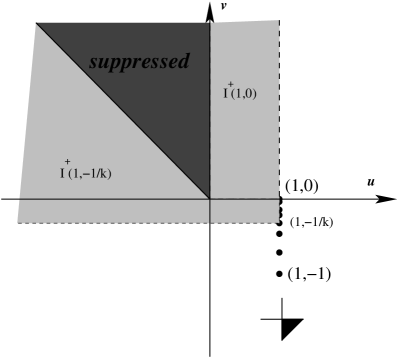
Figure 3: The left picture is the 2-dimensional spacetime $(V,\boldsymbol{\eta})$. We have coloured in grey the chronological future of a point of the sequence $\{(1,-1/k)\}_{k=1}^{\infty}$. The chronological future of $(1,0)$ is the grey region above the $u$ axis and positive $u$. The picture of the right describes the geometric construction needed to define $s_{uv}=l_{uv}/L_{uv}$.

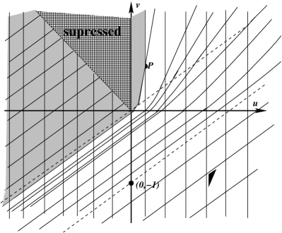
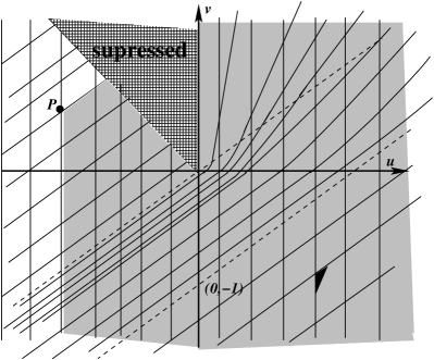
Figure 4: In these pictures we show the lightlike geodesics of $(V,{\bf g})$. The vertical lines are integral curves of $\vec{\boldsymbol{\xi}}_{2}$ whereas the oblique lines are the integral curves of $\vec{\boldsymbol{\xi}}_{1}$. In the left picture we have coloured in grey the causal future of a point $P$ lying in the first quadrant, whereas in the right picture the grey region corresponds to the causal past of a point $P$ now in the second one. In both cases these regions are closed sets. From these pictures we deduce that the causal future of any sequence of points approaching to $(0,0)$ converges toward the region $u<0$, $v>u$ whereas their causal past tends to the region $u>0$.

This example proves that theorem 2.1 does not hold if $V_{2}$ is causally simple or causally continuous. This raises the question as to why these two conditions behave differently under the action of causal mappings. The ultimate reason of this relies on the fact that causality conditions covered by theorem 2.1 only deal with global causal properties of the spacetime making them causality conditions in a strict sense (to see this observe that they can always be formulated in terms of a condition or conditions involving only causal curves, see e. g. [21, 1, 37]). As causal continuity and causal simplicity relate causal and topological properties of the differentiable manifold, they are not in the same footing as the other conditions. The moral is that although causal continuity and causal simplicity are not covered by theorem 2.1, definition 2.3 should not be affected by the existence of two spacetimes with the same causal structure but only one of them being causally simple.

4 New criteria for non-existence of causal mappings

In section 2 we saw some ways to disprove the existence of causal mappings. They involve a global causal property not shared by the Lorentzian manifolds under study and, essentially, they were reduced to two criteria: the standard causal hierarchy of spacetimes, theorem 2.1 (with the limitations pointed in subsection 3.2) and the nonexistence of horizons, proposition 2.3. Additionally, example 2.2 explains a property which can be used as a third criterion.

As we are going to see next, more elaborate criteria can be used in complex situations. The procedure is similar to what we did in section 2: we give a number of global causal properties on $V_{2}$ which are transferred to $V_{1}$ (or vice versa) if $V_{1}\prec V_{2}$, and this implies that $V_{1}\not\prec V_{2}$ if any of these properties fails in $V_{1}$.

In what follows, any hypersurface $S$ (or submanifold) will be considered smooth, embedded, connected and edgeless (thus without boundary). Recall that, for a subset of a spacetime $A\subseteq V$, the common past is defined by $\downarrow A\equiv\cap_{x\in A}I^{-}(x)$.

Proposition 4.1.

Assume that $V_{1}\prec V_{2}$ and that $V_{1}$ admits $j$ inextendible future-directed causal curves (or, in general, $j$ submanifolds at no point spacelike and closed as subsets of $V_{1}$) $\gamma_{i},i=1,\dots,j$ satisfying either of the following conditions:

1. $V_{1}=I^{+}(\gamma_{i})\cup\gamma_{i}\cup I^{-}(\gamma_{i})$.

2. $\gamma_{i}\subseteq\downarrow\gamma_{i+1}$, $\forall i=1,\dots,j-1$, $j>1$.

Then so does $V_{2}$.

Proof :    Denote by $\Phi:V_{1}\rightarrow V_{2}$ the causal mapping. From point (iv) of proposition 2.1 it is clear that the sets $\Phi(\gamma_{i})$, $i=1,\dots,j$ satisfy condition 1 in $V_{2}$ whenever $\gamma_{i}$, $i=1,\dots,j$ do in $V_{1}$. To prove the second point we have to use the property

$$\Phi(\downarrow A)\subseteq\downarrow\Phi(A),\ A\subset V_{1},$$

which again is a straightforward consequence of point (iv) of proposition 2.1.

Example 4.1.

As a simple application, we can show that there are infinitely many rectangles of $\mathbb{L}^{2}$, in standard Cartesian coordinates $(t,x)$, which are not isocausal (the example is obviously generalizable to $\mathbb{L}^{n}$, by using hypersurfaces at no point spacelike instead of causal curves). For each $L>0$, let $R_{L}=\{(t,x):t\in]0,L[,x\in]0,1[\}\subset\mathbb{L}^{2}$. Note that, if $L<L^{\prime}$, then $R_{L}\prec_{\Phi}R_{L^{\prime}}$, where $\Phi(t,x)=(L^{\prime}t/L,x)$. A set of $j$ curves satisfies both properties of proposition 4.1 if and only if $L\geq j$ (see figure 5). Thus, if $L^{\prime}-L\geq 1$ then $R_{L^{\prime}}\not\prec R_{L}$. This result can be refined if $L=1$ in which case we can actually show that $R_{1+\epsilon}\not\prec R_{1}\not\prec R_{1-\epsilon}$, for any $0<\epsilon<1$. To see this note that if $V_{1}\prec_{\Phi}V_{2}$ and $p\in V_{1}$ is any point such that $V_{1}=I^{+}(I^{-}(p))=I^{-}(I^{+}(p))$ then $\Phi(p)$ also satisfies these same properties. In the case of $R_{1}$ only the point $p=(1/2,1/2)$ satisfies previous conditions whereas there are infinitely many points for $R_{1+\epsilon}$ (a neighbourhood of its centre) and none for $R_{1-\epsilon}$.

Figure 5: The curves $\gamma_{1}$, $\gamma_{2}$, $\gamma_{3}$ of this picture meet both conditions of proposition 4.1. The dashed lines are the future boundaries of the common past of $\gamma_{2}$ and $\gamma_{3}$.

For the following result, recall that if $\Phi$ is a causal mapping then $\Phi^{-1}$ maps non-timelike vectors to non-timelike vectors.

Proposition 4.2.

Assume that $V_{1}\prec V_{2}$ and suppose that $V_{2}$ satisfies one of the following properties

1. There exists an acausal (resp. achronal; achronal and spacelike; a foliation by any of previous ones) hypersurface $S^{\prime}$, which is closed (resp. compact) as a subset of $V_{2}$.

2. There exists a hypersurface $S^{\prime}\subset V_{2}$ as in (1) such that $V_{2}\neq I^{+}(S^{\prime})\cup S^{\prime}\cup I^{-}(S^{\prime})$.

3. There are $k>1$ hypersurfaces $S^{\prime}_{j}\subset V_{2}$, $j=1,\dots k$ as in (1) such that no pair of them can be joined by a causal curve.

   Then the same property is satisfied by $V_{1}$. Moreover, if:

4. all the hypersurfaces in $V_{1}$ with any of the properties stated in (1) are homeomorphic,

   then so happens in $V_{2}$.

Proof :    We prove each case separately (in all cases we take as $\Phi:V_{1}\rightarrow V_{2}$ the diffeomorphism establishing the causal mapping).

(1)   If $S^{\prime}$ is the stated hypersurface of $V_{2}$ then by point $(\ref{point5})$ of proposition 2.1 $\Phi^{-1}(S^{\prime})$ has these same properties as a subset of $V_{1}$. Moreover if $S^{\prime}$ belongs to a foliation of $V_{2}$ then $\Phi^{-1}$ gives rise to a foliation of $V_{1}$ with the required properties.

(2).   If $V_{2}\neq I^{+}(S^{\prime})\cup S^{\prime}\cup I^{-}(S^{\prime})$ then

$$\Phi^{-1}(I^{+}(S^{\prime})\cup S^{\prime}\cup I^{-}(S^{\prime}))=\Phi^{-1}(I^{+}(S^{\prime}))\cup\Phi^{-1}(S^{\prime})\cup\Phi^{-1}(I^{-}(S^{\prime}))\neq V_{1}.$$

The result is now a consequence of the property

$$I^{+}(S^{\prime})\supseteq\Phi(I^{+}(\Phi^{-1}(S^{\prime}))),$$

(and analogously for $I^{-}$) which tells us that $\Phi^{-1}(S^{\prime})$ is the sought hypersurface.

(3).   If no pair of the set $\{S^{\prime}_{j}\}$, $j=1,\dots k$ can be joined by a causal curve then the same is true of the hypersurfaces $\Phi^{-1}(S^{\prime}_{j})$.

(4).  Pick any pair of acausal (resp. achronal, achronal and spacelike) closed (resp. compact) hypersurfaces $S^{\prime}_{1}$, $S^{\prime}_{2}\subset V_{2}$. The hypersurfaces $\Phi^{-1}(S^{\prime}_{1})$, $\Phi^{-1}(S^{\prime}_{2})$ are homeomorphic by assumption, and then so are $S^{\prime}_{1}$, $S^{\prime}_{2}$, since $\Phi$ is a homeomorphism.

Now, we present some examples showing how to apply conditions of this last proposition, and postpone further examples to the next section.

Example 4.2.

A simple spacetime complying with property (2) is $\mathbb{L}^{2}$ with any of the quadrants defined by Cartesian coordinate axes removed. If, instead of a quadrant, we remove the $m$ regions defined by $[j,j+a]\times]-\infty,0]$, $j=0,\dots m-1$, $a<1$ then property (3) is satisfied, see figure 6. Note that any of these spacetimes (denoted generically by $V$) is diffeomorphic to $\mathbb{L}^{2}$ but, as $\mathbb{L}^{2}$ does not fulfill either property, $\mathbb{L}^{2}\not\prec V$ (the opposite causal mapping is also forbidden because $V$ is never globally hyperbolic).

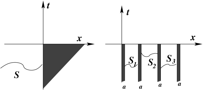
Figure 6: Examples of spacetimes satisfying properties (2) and (3). All the regions in dark grey are suppressed. In the left picture $V\neq I^{+}(S)\cup S\cup I^{-}(S)$ while in the right picture no pair of the set $\{S_{1},S_{2},S_{3}\}$ can be joined by a causal curve.

Example 4.3.

Another explicit example of property (3) yields infinitely many globally hyperbolic open subsets of $\mathbb{L}^{2}$ which are not isocausal, extending previous results on Lorentz surfaces [43]. We again resort to $\mathbb{L}^{2}$ but now in null coordinates $\{u,v\}$, $\boldsymbol{\eta}=2dudv,$ and we define the “stairway-shaped” open regions $\Omega_{m}$, $m\in\mathbb{N}$ (see figure 7). A Cauchy hypersurface can be obtained by drawing a spacelike curve from $(0,1)$ to $(1,0)$. All these regions comply with property (3) (the set of hypersurfaces $S^{\prime}_{j}$ are shown in the picture). The greatest number of such hypersurfaces is given by $m$ for each $\Omega_{m}$ so proposition 4.2 tells us that $\Omega_{m}\not\prec\Omega_{m^{\prime}}$ if $m<m^{\prime}$. In particular there is no conformal relation between $\Omega_{m}$ and $\Omega_{m^{\prime}}$ if $m\neq m^{\prime}$, and thus there are infinitely many simply connected Lorentz surfaces in the sense of [43] (see this reference for a different proof of this last result). Summing up, simple bi-dimensional diffeomorphic globally hyperbolic spacetimes with different causal structures are found.

In this same context, consider the manifold $\Omega_{1}$ (a square in the plane $u-v$) and define the manifold $\Omega^{*}_{1}$ as the open region of $\mathbb{L}^{2}$ shown in figure 7. Clearly there are acausal closed hypersurfaces in $\Omega^{*}_{1}$ fulfilling property (2) (the hypersurface $S^{\prime}$ of the figure is an example) but none in $\Omega_{1}$ so $\Omega_{1}\not\prec\Omega^{*}_{1}$.

Figure 7: The picture of the left is the globally hyperbolic set $\Omega_{8}$ where a set of hypersurfaces complying with point (3) of proposition 4.2 has been drawn. The picture of the right is $\Omega^{*}_{1}$.

Example 4.4.

Property (4) is satisfied by de Sitter spacetime $\mathbb{S}_{1}^{n}$ if the hypersurfaces are considered compact (see proposition 5.6 below), but it is not if they are only closed as a subset. In fact, not only does $\mathbb{S}_{1}^{n}$ admit compact spacelike (achronal) hypersurfaces, but also non-compact ones which are closed as a subset of $\mathbb{S}_{1}^{n}$. This can be easily seen if we resort to the representation of $\mathbb{S}_{1}^{n}$ as a unit sphere of $\mathbb{L}^{n+1}$ with respect to the pseudo-distance induced by the Lorentzian metric. The intersection of $\mathbb{S}_{1}^{n}$ with a null hyperplane of $\mathbb{L}^{n+1}$ through the origin is then one of such hypersurfaces.

As we will see in the next section, property (4), even in the case of hypersurfaces only closed as a subset (but non necessarily compact a priori), holds in spacetimes which include the standard stationary spacetimes (proposition 5.4, remark 5.1) and some generalizations of Robertson-Walker models (proposition 5.6). Thus, proposition 4.2 will forbid the isocausality of any of these spacetimes and $\mathbb{S}_{1}^{n}$.

It is not difficult to give other examples which show the applicability of previous criteria, as well as to find new criteria by making simple variations of proposition 4.2 (see, for example, remark 5.4).

5 Causal structures in smooth product spacetimes

5.1 Smooth time-product spacetimes

Consider a $n$-dimensional spacetime $(V,{\bf g})$ with base manifold the smooth product $V=I\times S$ where $I$ is an interval of $\mathbb{R}$, $S$ is a $n-1$ dimensional manifold and $t:V\rightarrow I$ the natural projection. If each slice $\{t\}\times S$ is spacelike as an embedded submanifold of $V$ and the vector field $\partial/\partial t$ is timelike (and will be assumed future-directed), then the metric ${\bf g}$ can be written globally as

$${\bf g}=\rho dt\otimes dt+{\bf\Omega}\otimes dt+dt\otimes{\bf\Omega}-{\bf h}[t],\ t\in I,$$ (5.1)

where $\rho\in C^{1}(V)$ is positive, ${\bf h}[t]$ is a family of Riemannian metrics on $S$ and $\boldsymbol{\Omega}$ is a 1-form on $I\times S$. The resulting spacetime is called a smooth time-product. Notice that one can assume $I=\mathbb{R}$ without loss of generality, but the interval $I$ will be maintained some times for convenience. A first interesting case are standard stationary spacetimes, studied in subsection 5.3. Another case, even more interesting, is when $\boldsymbol{\Omega}=0$ which entails

$${\bf g}=\rho dt^{2}-{\bf h}[t],\ t\in I.$$ (5.2)

We shall employ the terminology 1-timelike separable spacetimes for these Lorentzian manifolds. Locally, any spacetime can be written as in (5.2), even with $\rho\equiv 1$ (the role of $\rho^{1/2}dt$ can be played by any integrable timelike 1-form); thus, expressions as (5.1), (5.2) are restrictive only from a global viewpoint. However, metrics such as (5.1), and, especially, those which are 1-timelike separable, represent many physically interesting spacetimes and they arise in general settings. For instance, it has been recently shown that, for any globally hyperbolic spacetime, the metric tensor has the form (5.2) [5, 6], and in this case $t$ can be set to a time function with Cauchy hypersurfaces $t=$const (some extensions to stably causal spacetimes are also possible, see [6, 36]).

5.2 Arrival time functions

It is not difficult to check in certain particular cases of (5.1) whether there are curves with no particle horizons. To that end, following [32] we define the future arrival time function as the map $T^{+}:V\times S\rightarrow[0,\infty]$ given by

$$T^{+}((t_{1},x_{1}),x_{2})=\mbox{Inf}\{t-t_{1}:(t_{1},x_{1})\leq(t,x_{2}),t\in I\},\ \quad t_{1}\in I,\ x_{1},x_{2}\in S,$$

and dually for the past arrival time function $T^{-}$. Recall that if we define the comoving trajectory at $x_{2}$ as $R_{x_{2}}=\{(t,x_{2}):t\in I\}$, then, if $I=(a,b)\subseteq\mathbb{R}$:

$$\{t\in I:(t,x_{2})\in R_{x_{2}}\cap I^{+}(t_{1},x_{1})\}=(t_{1}+T^{+}((t_{1},x_{1}),x_{2}),b).$$

Thus, the meaning of the arrival functions is the following:

Proposition 5.1.

In a smooth time-product spacetime we have

$$(t_{1},x_{1})\ll(t_{2},x_{2})\Longleftrightarrow T^{+}((t_{1},x_{1}),x_{2})<t_{2}-t_{1}\Longleftrightarrow T^{-}((t_{2},x_{2}),x_{1})<t_{2}-t_{1}.$$

The study of time arrival functions permits us to draw interesting conclusions about global causal properties of smooth time-product spacetimes; general properties and applications have been studied in [34, 32]. In particular, if the hypersurfaces $t=$const are Cauchy hypersurfaces then $T^{\pm}$ are continuous functions in their variables. Arrival time functions are related to the existence of particle horizons for comoving trajectories (for simplicity, we put $I=\mathbb{R}$).

Proposition 5.2.

Consider a smooth time-product spacetime $V=\mathbb{R}\times S$. Fixed $x_{0}$, the comoving trajectory $R_{x_{0}}$ has no past (resp. future) particle horizon if and only if $T^{+}(p,x_{0})<\infty$, $\forall p\in V$ (resp. $T^{-}(p,x_{0})<\infty$).

Proof :    According to proposition 5.1 the condition on $T^{+}$ is clearly equivalent to $(t_{1},x_{1})\leq(t_{0},x_{0})$ for any point $p\equiv(t_{1},x_{1})$ and some $t_{0}\in\mathbb{R}$.

In particular, when $V_{1},V_{2}$ are time-product spacetimes and $V_{1}\prec_{\phi}V_{2}$ for a causal mapping which preserves the decomposition (5.1) (i.e., which maps each comoving trajectory $\{(t,x):t\in\mathbb{R}\}$ in $V_{1}$ into a comoving trajectory of $V_{2}$) then the finiteness of $T^{+}$ (resp. $T^{-}$) for $V_{1}$ implies the finiteness for $V_{2}$. Recall that sufficient conditions for the finiteness of $T^{\pm}$ are easy to obtain [32] (see also propositions 5.3, 5.5 below).

5.3 Standard stationary spacetimes

A smooth time-product spacetime $I\times S$ as in (5.1) is called standard stationary if $I=\mathbb{R}$ and all the elements of ${\bf g}$ are independent of $t$, i.e., $\vec{\boldsymbol{\xi}}=\partial/\partial t$ satisfies $\pounds_{\vec{\boldsymbol{\xi}}}\rho=0$, $\pounds_{\vec{\boldsymbol{\xi}}}\boldsymbol{\Omega}=0$ and ${\bf h}[t]\equiv{\bf h}$. Locally, any stationary spacetime (i.e., a spacetime which admits a timelike Killing vector field $\vec{\boldsymbol{\xi}}$) looks like a standard one. If the metric (5.1) is both, standard stationary and 1-timelike separable then the spacetime is called static standard (see [35] for a survey).

In such stationary $\mathbb{R}\times S$, any (non-constant) curve $\alpha$ contained in $S$ joining two fixed points $x_{0},x_{1}$ yields a unique future-directed (resp. past-directed) lightlike curve $\gamma$ connecting a fixed $(t_{0},x_{0})$ with some $(t_{1},x_{1})$, $t_{1}>t_{0}$ by means of the definition $\gamma:t\rightarrow(\tau(t),\alpha(t))$, $t\in[t_{0},t_{1}]$ where $\tau(t)$ satisfies the differential equation $\rho^{2}\tau^{\prime 2}+2\tau^{\prime}{\bf\Omega}(\alpha^{\prime})-{\bf h}(\alpha^{\prime},\alpha^{\prime})=0$ with ${}^{\prime}\equiv d/dt$. Thus:

Proposition 5.3.

In a standard stationary spacetime, both arrival functions $T^{+},T^{-}$ are always valued in $\mathbb{R}$.

Recall also that property (1) of proposition 4.2 is satisfied in standard stationary spacetimes where, by definition, a foliation by achronal and spacelike hypersurfaces exists. These spacetimes do not satisfy property (2) but they do satisfy property (4).

Proposition 5.4.

In a standard stationary spacetime $V=(\mathbb{R}\times S,{\bf g})$, any smooth achronal hypersurface $\hat{S}$ which is closed (as a subset of $\mathbb{R}\times S$) is diffeomorphic to $S$.

Proof :    As the vector field $\vec{\boldsymbol{\xi}}$ is complete its flow defines a local diffeomorphism $\Psi:\hat{S}\rightarrow S$, which is injective by achronality. Its image is then an open subset $\Psi(\hat{S})\subseteq S$. To check that it is closed and, thus, the equality holds, consider a sequence $\{x_{m}\}_{m=1}^{\infty}$ on $\Psi(\hat{S})$ which converges to a boundary point $x_{0}$. Take the sequence $\{\Psi^{-1}(x_{m})\}_{m=1}^{\infty}\subset\hat{S}$ and define the quantities $T^{\pm}(\Psi^{-1}(x_{1}),x_{m})$, $m\in\mathbb{N}$. By proposition 5.3 all of them are finite and even more they are bounded by a constant independent of $m$. To see this last assertion, note that $T^{\pm}(\Psi^{-1}(x_{1}),x)\leq T^{\pm}(\Psi^{-1}(x_{1}),x_{0})+C$ where $x$ lies in a neighbourhood of $x_{0}$ and $C$ is a constant. The main consequence of this is that all the values of $t$ for all the points of the sequence $\{\Psi^{-1}(x_{m})\}_{m=1}^{\infty}$ are in a bounded interval which implies that, since $\hat{S}$ is closed, $\{\Psi^{-1}(x_{m})\}_{m=1}^{\infty}$ lies in a compact subset of $V$. Thus, it has a subsequence convergent to a point $\bar{x}_{0}\in\hat{S}$, and $x_{0}=\Psi(\bar{x}_{0})\in\Psi(\hat{S})$, as required.

Remark 5.1.

1. If $S$ is simply connected, the global condition “achronal” can be weakened to “locally achronal” (i.e., with the induced metric not being Lorentzian at any point; obviously, this is fulfilled if $S$ is either spacelike or degenerate at any point), because this condition is enough to prove that $\Psi$ is a covering map (see theorem 4.4 of [20] for a proof in a more general setting). Nevertheless, if $S$ is not simply connected the achronality cannot be weakened (just think in the Lorentzian cylinder, $\mathbb{R}\times S$, $S=S^{1}$, and take $\hat{S}$ as a spacelike helix).

2. Remarkably, Harris and Low in [20] proved a more general result than proposition 5.4: if a spacetime fulfills (i) $V$ admits a congruence ${\cal F}$ of inextensible timelike curves such that for any curve $\gamma\in{\cal F}$ we have that $I^{\pm}(\gamma)=V$, and (ii) there exist an achronal and properly embedded hypersurface $S$ in $V$, then any other achronal hypersurface in $V$ is diffeomorphic to $S$ (recall that “properly embedded” implies our assumption “closed as a subset”). A related result with the extra assumption of timelike or null geodesic completeness can be found in theorem 3 of [16].

Notice that in de Sitter spacetime $\mathbb{S}_{1}^{n}$ the property stated in proposition 5.4 does not hold (example 4.4). Thus, as a consequence of proposition 4.2 one has the following result, applicable in particular when $V$ is Einstein static universe.

Corollary 5.1.

If $V$ is any standard stationary spacetime, $V\not\prec\mathbb{S}^{n}_{1}$.

5.4 General estimate for 1-timelike separable spacetimes

Next, we give a general estimate which ensures the existence of causal mappings between 1-timelike separable spacetimes. We can assume that the base manifold is always the same and add the superscripts or subscripts $1$ and $2$ on the elements of the metric (5.2) for each one of the two 1-timelike separable spacetimes.

Theorem 5.1.

Let $(V,{\bf g}_{1})$, $(V,{\bf g}_{2})$ be 1-timelike separable spacetimes with respect to the same decomposition of $V$ written as $V=I\times S$. If $I$ is an unbounded interval then a sufficient set of conditions for ${\bf g}_{1}\prec{\bf g}_{2}$ is the following:

1. $$\begin{array}[]{c}k=\mbox{\large Inf}\\ \mbox{\footnotesize$t_{1},t_{2}\in I,x\in S$}\end{array}\frac{\rho_{2}(t_{2},x)}{\rho_{1}(t_{1},x)}>0,$$

2. The norm $||\hat{\bf h}_{2}[t]||$ of the endomorphism $\hat{\bf h}_{2}[t]$ with respect to ${\bf h}_{1}[t]$, defined in the tangent space $T_{x}S$ of any point $x\in S$ by the condition

   $${\bf h}_{2}[t](\vec{\boldsymbol{u}},\vec{\boldsymbol{v}})={\bf h}_{1}[t](\hat{\bf h}_{2}[t]\vec{\boldsymbol{u}},\vec{\boldsymbol{v}}),\ \forall\vec{\boldsymbol{u}},\vec{\boldsymbol{v}}\in T_{x}S$$ (5.3)

   is bounded by a constant independent of $p\equiv(t,x)\in V$.

Proof :    This is proven by the explicit construction of a causal mapping $\Phi:(V,{\bf g}_{1})\rightarrow(V,{\bf g}_{2})$. We will perform the proof for $I=\mathbb{R}$ but nothing essential changes if $I=]a,\infty[$ or $I=]-\infty,a[$ for some $a\in\mathbb{R}$. Define $\Phi$ by means of $\Phi:(t,x)\mapsto(l(t),x)$ where $l(t)$ is a strictly increasing $C^{1}$ function and $x\in S$. Then

$$\Phi^{*}{\bf g}_{2}=\rho_{2}(l(t),x)l^{\prime}(t)^{2}dt^{2}-{\bf h}_{2}[l(t)].$$

The endomorphism associated to $\Phi^{*}{\bf g}_{2}$ is in matrix form (naturally associated to (5.2))

$$\widetilde{\Phi^{*}{\bf g}}_{2}=\left(\begin{array}[]{cc}\frac{\rho_{2}(l(t),x)}{\rho_{1}(t,x)}l^{\prime}(t)^{2}&\\ &\hat{\bf h}_{2}[t]\end{array}\right).$$

According to proposition 2.5, we deduce that $\Phi^{*}{\bf g}_{2}$ is a causal tensor if and only if

$$\frac{\rho_{2}(l(t),x)}{\rho_{1}(t,x)}l^{\prime}(t)^{2}\geq|\lambda_{i}(p)|,\ i=1,\dots,n-1,$$ (5.4)

where the $\lambda_{i}(p)$’s are the eigenvalues of $\hat{\bf h}_{2}[t]$. The condition on $||\hat{\bf h}_{2}[t]||$ ensures that these eigenvalues will be functions of $p$ bounded by a constant

$$\begin{array}[]{ccc}N=&Sup&\!\!\!||\hat{\bf h}_{2}[t](x)||.\\ &(t,x)\in V&\end{array}$$

On the other hand the inequality

$$\frac{\rho_{2}(l(t),x)}{\rho_{1}(t,x)}l^{\prime}(t)^{2}>N,$$

which implies (5.4), will hold whenever

$$l^{\prime}(t)\geq\sqrt{\frac{N}{k}},$$

in particular, by the choice $l(t)=(N/k)^{1/2}t$.

Interchanging the roles of ${\bf g}_{1}$ and ${\bf g}_{2}$, conditions for ${\bf g}_{2}\prec{\bf g}_{1}$ are obtained and, then:

Corollary 5.2.

Two 1-timelike separable spacetimes $(V,{\bf g}_{1})$, $(V,{\bf g}_{2})$, $V=I\times S$, written as in (5.2) with unbounded $I$, are causally equivalent if, for some positive constants $N,N^{\prime},k,k^{\prime}>0$:

$$k\leq\frac{\rho_{1}(t_{2},x)}{\rho_{2}(t_{1},x)}\leq k^{\prime},\ \forall t_{1},t_{2}\in I,\ \forall x\in S,\quad N\leq||\hat{\bf h}_{2}[t](x)||\leq N^{\prime},\quad\forall(t,x)\in I\times S.$$

Remark 5.2.

The results have been formulated with general functions $\rho$ to make them more easily applicable. Nevertheless, as the existence of causal mappings is a conformal invariant, the metric of (5.2) can be rescaled by $1/\rho$, and all the results re-formulated assuming that $\rho\equiv 1$. In this case we are only left with the second condition of theorem 5.1 and corollary 5.2 and, in fact, the so-obtained bounds are more general. In a similar way, if $I$ were bounded then the change $t=f(\bar{t})$ with $\bar{t}$ ranging in an unbounded interval $J$ would bring the metrics into a form in which conditions of theorem 5.1 could be checked.

5.5 GRW spacetimes

In previous subsection, we have obtained a general set of sufficient conditions for the causal equivalence of arbitrary timelike 1-separable spacetimes. Nevertheless, previous results (like those for stationary spacetimes or the example 4.1) suggest the existence of many different causal structures, even in the globally hyperbolic case. To show this more explicitly, we focus now on a particular case of spacetimes.

Generalized Robertson Walker spacetimes (GRW in short) are (1-timelike separable) warped products defined by:

$$V=I\times_{f}S,\quad{\bf g}=dt^{2}-f^{2}(t){\bf h},$$ (5.5)

where ${\bf h}$ is a Riemannian metric on the $(n-1)$-manifold $S$, and $f$ is a positive real function. Notice that the change

$$T(t)=\int_{t_{0}}^{t}\frac{ds}{f(s)},$$ (5.6)

brings the above metric into the form

$${\bf g}=f^{2}(t(T))(dT^{2}-{\bf h})$$ (5.7)

where $T$ varies in a new interval, $I_{T}$. Thus, any GRW is conformal to a metric product; in particular, it is globally hyperbolic if and only if $(S,{\bf h})$ is complete (see [33] for further properties). The GRW spacetime will be called spatially closed if $S$ is compact (without boundary); recall that in this case the spacetime is globally hyperbolic.

Reasoning as for standard stationary spacetimes in proposition 5.3, we have:

Proposition 5.5.

In any GRW spacetime $I\times_{f}S$ with $I=\mathbb{R}$ and $f$ bounded, both arrival functions $T^{+},T^{-}$ are always valued in $\mathbb{R}$.

(Clearly, the result still holds if $f$ only satisfies $\int_{t_{0}}^{\infty}1/f=\infty,\int^{t_{0}}_{-\infty}1/f=\infty$.)

GRW spacetimes do not always satisfy point (4) of proposition 4.2. In fact, de Sitter spacetime $\mathbb{S}^{n}_{1}$, which can be written as the spatially closed GRW spacetime $\mathbb{R}\times_{\cosh}\mathbb{S}^{n-1}$, is a counterexample (example 4.4). Nevertheless, the following result shows that the property is still satisfied in interesting cases.

Proposition 5.6.

Consider a spatially closed GRW $I\times_{f}S$, and any smooth achronal hypersurface $\hat{S}$. Then, $\hat{S}$ is diffeomorphic to $S$ if one of the two following conditions hold:

1. $\hat{S}$ is compact.

2. $I=\mathbb{R}$, $f$ is bounded and $\hat{S}$ is closed as a subset of $I\times S$.

Proof :    Let $\Pi:V\rightarrow S$, $\Pi_{R}:V\rightarrow\mathbb{R}$ be the natural projections.

1. As the restriction of $\Pi$ to $S$ is a local diffeomorphism, necessarily the restriction $\Pi|_{\hat{S}}:\hat{S}\rightarrow S$ is a covering map. But the acausality of $S$ implies that this covering map has only one leaf, and hence it is a diffeomorphism.

2. From the previous part, it is enough to prove that the hypotheses imply the compactness of $\hat{S}$. For any point $p\in\hat{S}$ the function defined by $T^{+}(p,\cdot):S\rightarrow[0,\infty]$ takes values in $\mathbb{R}^{+}$ (proposition 5.5) and, as it is continuous [34, proposition 2.2], its image is bounded in $\mathbb{R}$.

   The acausality of $\hat{S}$, implies that the interval $\Pi_{R}(\hat{S})$ is also bounded. To see this assume the contrary and pick a point $p_{1}=(t_{1},x_{1})\in\hat{S}$ such that $|\Pi_{R}(p_{1})-\Pi_{R}(p)|>T^{\pm}(p,x_{1})$; this inequality means that there exists a timelike curve joining $p$ and $p_{1}$, which contradicts the achronality of $\hat{S}$. Therefore $\hat{S}$ lies in a compact subset of $V$. Since $\hat{S}$ is closed, it is compact too, as required.

Remark 5.3.

As in remark 5.1, when $S$ is simply connected, “achronality” can be weakened to “local achronality”.

Again, these results are applicable to de Sitter spacetime (and, in particular, for comparisons with Einstein static Universe, regarded as a GRW spacetime).

Corollary 5.3.

If $V=\mathbb{R}\times_{f}\mathbb{S}^{n-1}$ is a GRW spacetime with $f$ bounded, then $V\not\prec\mathbb{S}^{n}_{1}$.

In order to obtain further conditions for the isocausality of spatially closed GRW, notice first that, as a consequence of corollary 5.2:

Lemma 5.1.

Two spatially closed GRW spacetimes $V_{i}=I\times_{f_{i}}S$ with the same base manifold $I\times S$ and $I$ unbounded, are isocausal if

$$0<\mbox{ Inf}(f_{i})\leq\mbox{ Sup}(f_{i})<\infty\ ,\quad i=1,2.$$

Proof :    Apply corollary 5.2 taking into account that, for any point $(t,x)$,

$$\hat{\bf h}_{2}[t](x)=\frac{f_{2}(t)}{f_{1}(t)}\tilde{\alpha}_{x},$$

where $\tilde{\alpha}_{x}$ is the endomorphism associated to a (fixed) Euclidean scalar product of the tangent $T_{x}S$ independent of $t$. So, the compactness of $S$ yields the required inequality (5.4) for the eigenvalues of $\hat{\bf h}_{2}$.

Proposition 5.7.

The causal structure of a spatially closed GRW spacetime $I\times_{f}S$ with $I$ unbounded and $0<\mbox{ Inf}(f)\leq\mbox{ Sup}(f)<\infty$ is stable in the $C^{0}$ topology.

Proof :    Let ${\bf g}$ be the warped metric, put $f_{1}=2f,f_{2}=f/2$, and let ${\bf g}_{i}$ be the metric of the corresponding $I\times_{f_{i}}S$. The metrics with light cones strictly wider than ${\bf g}_{1}$ and strictly narrower than ${\bf g}_{2}$ constitute a $C^{0}$ neighbourhood of ${\bf g}$. Obviously, for any metric ${\bf g}^{\prime}$ in such a neighbourhood ${\bf g}_{1}\prec_{id}{\bf g}^{\prime}\prec{\bf g}_{2}$ but, from lemma 5.1, ${\bf g}_{1}\sim{\bf g}_{2}$.

Of course proposition 5.7 can be trivially extended to the case in which the intervals $I$ are not equal in both spacetimes, i.e., the base manifolds are $I_{j}\times S$, $j=1,2$, but both $I_{j}$ are unbounded with the same (upper, lower or both) infinite extremes. $S$ can also be replaced by two diffeomorphic compact manifolds $S_{j}$ but, essentially, no further generality is gained. Nevertheless, the restriction of the extremes being unbounded must hold. Let us see this necessity first in the simple case of product metrics. Notice that the completeness assumption for ${\bf g}_{2}$ in the following result is written only for simplicity, and holds automatically if $S$ is compact.

Lemma 5.2.

Consider the product spacetimes

$$V_{1}=(I_{1}\times S,\ {\bf g}_{1}=dt^{2}-{\bf h}_{1}),\ V_{2}=(I_{2}\times S,\ {\bf g}_{2}=dt^{2}-{\bf h}_{2}),$$

where ${\bf h}_{1},{\bf h}_{2}$ are Riemannian metrics on $S$, ${\bf h}_{2}$ complete, and $I_{1},I_{2}\subseteq\mathbb{R}$ are two open intervals. If $I_{2}$ is upper (resp. lower) bounded but $I_{1}$ is not then ${\bf g}_{1}\not\prec{\bf g}_{2}$.

Proof :    We only perform the proof for the case in which $I_{2}=]0,\infty[$, and $I_{1}=\mathbb{R}$ (the proof remains essentially equal for any other interval combinations). By proposition 2.3, it is enough to show that there is an inextendible causal curve $\gamma$ in $V_{1}$ without particle horizon, whereas no such curve exist in $V_{2}$. In fact, from propositions 5.2, 5.5, the curve $\gamma(t)=(t,x_{0}),t\in\mathbb{R}$ in $V_{1}$ satisfies the required condition. To check the nonexistence of such a $\gamma$ for $V_{2}$, notice that, as $\gamma$ would be causal, it can be reparametrized as $\gamma(t)=(t,x(t)),t>0$ with ${\bf h}_{2}(x^{\prime}(t),x^{\prime}(t))\leq 1$. From the completeness of ${\bf h}_{2}$, there exists the limit lim${}_{t\rightarrow 0}x(t)=x_{0}$. But $V_{2}$ can be regarded as an open subspace of $(\mathbb{R}\times S,dt^{2}-{\bf h}_{2})$ and, then, $I^{+}(\gamma)=I^{+}(0,x_{0})\neq I_{2}\times S$.

As any GRW spacetime is conformally equivalent to a product one, combining the associate change of variable (5.6) with lemma 5.2 we have:

Proposition 5.8.

Consider two GRW spacetimes $I_{i}\times_{f_{i}}S$

$$V_{1}=I_{1}\times S,\ {\bf g}_{1}=dt^{2}-f_{1}^{2}(t){\bf h}_{1},\ V_{2}=I_{2}\times S,\ {\bf g}_{2}=dt^{2}-f_{2}^{2}(t){\bf h}_{2},$$

where $I_{1},I_{2}\subseteq\mathbb{R}$ are two open intervals $I_{i}=]a_{i},b_{i}[$ and ${\bf h}_{1}$, ${\bf h}_{2}$ complete Riemannian metrics. Suppose also that $c_{i}\in I_{i}$ exists, such that one of the integrals

$$\int_{a_{i}}^{c_{i}}\frac{dt}{f_{i}(t)},\quad\int_{c_{i}}^{b_{i}}\frac{dt}{f_{i}(t)},$$

is infinite for $i=1$ and finite for $i=2$. Then ${\bf g}_{1}\not\prec{\bf g}_{2}$.

Example 5.1.

Consider the family of GRW spacetimes with $f(t)=t^{a}$, $a\in\mathbb{R}$, $t\in]0,\infty[$ and $S=\mathbb{R}^{n-1}$. Since

$$\int_{0}^{c}t^{-a}dt<\infty,\ \mbox{if}\ a<1,\int_{0}^{c}t^{-a}dt=\infty,\ \mbox{if}\ a\geq 1,$$

$$\int_{c}^{\infty}t^{-a}dt=\infty,\ \mbox{if}\ a\leq 1,\int_{c}^{\infty}t^{-a}dt<\infty,\ \mbox{if}\ a>1,$$

for any $c>0$ we deduce that spacetimes with $a<1,a=1,a>1$ are never isocausal.

Proposition 5.8 allows us to distinguish different causal structures in GRW spacetimes. When combined with lemma 5.1 and proposition 5.7, we can give a first classification of spatially closed GRW spacetimes. In order to give concrete physical examples, we will assume that the slices $t=$ constant are spheres, but the scheme works equally well for any type of compact slices.

Theorem 5.2.

Consider any GRW spacetime $V=I\times_{f}S$ with $S$ diffeomorphic to a $(n-1)-$sphere. Then $V$ is isocausal to one and only one of the following four types of product spacetimes:

1. $\mathbb{R}\times\mathbb{S}^{n-1}$, i.e., Einstein static universe, with metric

   $${\bf g}=dt^{2}-d\boldsymbol{\Omega}_{n-1}^{2},\ t\in\mathbb{R},$$

   where $d\boldsymbol{\Omega}_{n-1}^{2}$ represents the metric of the unit ($n-1$)-dimensional sphere.

2. $]0,\infty[\times\mathbb{S}^{n-1}$ with metric

   $${\bf g}=dt^{2}-\exp(2\alpha t)d\boldsymbol{\Omega}^{2}_{n-1},\ t\in\mathbb{R},\ \alpha<0.$$

3. $]-\infty,0[\times\mathbb{S}^{n-1}$. The metric is as in (ii) but now $\alpha>0$.

4. $]0,L[\times\mathbb{S}^{n-1}$, for some $L>0$.

In the three first cases, the causal structure is $C^{r}$-stable in the set of all the metrics on $I\times S$. Moreover, causal structures belonging to the above cases can be sorted as follows

$$\mbox{\em coset}({\bf g}_{iv})\preceq\left\{\begin{array}[]{c}\mbox{\em coset}({\bf g}_{ii})\\ \mbox{\em coset}({\bf g}_{iii})\end{array}\right\}\preceq\mbox{\em coset}({\bf g}_{i}),$$

where the roman subscripts mean that the representing metric belongs to the corresponding point of the above description.

Proof :    Only the sorting of the causal structures remains to be proved. To that end we cast the representative metric of each causal structure in the form of (5.7) obtaining

$${\bf g}_{i}=dt_{1}^{2}-d\boldsymbol{\Omega}^{2}_{n-1},\ t_{1}\in]-\infty,\infty[$$

$${\bf g}_{ii}=\frac{1}{\alpha^{2}t_{2}^{2}}(dt_{2}^{2}-d\boldsymbol{\Omega}^{2}_{n-1}),\ t_{2}\in]0,\infty[,\ \ {\bf g}_{iii}=\frac{1}{\alpha^{2}t_{3}^{2}}(dt_{3}^{2}-d\boldsymbol{\Omega}^{2}_{n-1}),\ t_{3}\in]-\infty,0[,$$

$${\bf g}_{iv}=dt^{2}_{4}-d\boldsymbol{\Omega}^{2}_{n-2},\ t_{4}\in]0,L[.$$

¿From these expressions it is not difficult to show that ${\bf g}_{iv}\prec{\bf g}_{iii}\prec{\bf g}_{i}$ and ${\bf g}_{iv}\prec{\bf g}_{ii}\prec{\bf g}_{i}$. Explicit causal mappings are (in all the cases only the time coordinate is involved)

$$t_{2}=A\tan\left(\frac{\pi t_{4}}{2L}\right),t_{3}=A\tan\left(\frac{\pi(t_{4}-L)}{2L}\right),\ A\geq\frac{2L}{\pi},$$

$$t_{1}=Bt_{2}-\frac{A}{t_{2}},\ t_{1}=Bt_{3}-\frac{A}{t_{3}},\ A>0,\ B>1.$$

Remark 5.4.

Note that the first three classes comprise each a single causal structure, whereas the fourth one contains more. To see it easily for $n=2$, consider example 4.1 but instead of rectangles $R_{L}$ take the cylinders $C_{L}=]0,L[\times\mathbb{S}^{1}$. If $L<L^{\prime}$ then $C_{L}\prec C_{L^{\prime}}$, but the converse does not necessarily hold. In fact, for $L=\pi$ we have: $C_{\pi+\epsilon}\not\prec C_{\pi}\not\prec C_{\pi-\epsilon}$, for any $\epsilon\in]0,\pi[$. This is so because, in $C_{\pi+\epsilon}$ there are timelike curves $\gamma$ which satisfy $V=J^{+}(\gamma)\cup J^{-}(\gamma)$ (essentially property (i) of proposition 4.1), in $C_{\pi}$ no timelike curve satisfies this property, but a lightlike curve $\gamma$ (in fact, any lightlike geodesic) satisfy $V=\overline{J^{+}(\gamma)\cup J^{-}(\gamma)}$, and in $C_{\pi-\epsilon}$ no causal curve satisfies the property. This can be generalized to any dimension $n>2$. For example, if $C_{L}^{n}=]0,L[\times\mathbb{S}^{n-1}$ the relation $C^{n}_{\pi}\not\prec C^{n}_{\pi-\epsilon}$ follows because $C^{n}_{\pi}=J^{-}(J^{+}(\gamma))$ (resp. $C^{n}_{\pi-\epsilon}\neq J^{-}(J^{+}(\gamma))$, for any inextendible causal curve $\gamma$.

Remarkably, de Sitter Universe

$$ds^{2}=dt^{2}-\cosh^{2}td\boldsymbol{\Omega}^{2}_{n-1},\ t\in\mathbb{R}.$$

belong to this last class, with $L=\pi$. In fact, from (5.6),

$$L=\int_{-\infty}^{\infty}\frac{dt}{\cosh(t)}=\pi.$$

Notice that small modifications of $f(t)=\cosh(t)$ may change the value of the integral and, thus, the causal structure. Formally, recall that, as $\mathbb{S}^{n-1}$ is compact, any neighbourhood of the de Sitter metric for any $C^{r}$-Whitney topology must contain functions $f$ which satisfy, say, $f(t)\geq\cosh(t)$ (resp. $f\leq\cosh(t)$), $f(t_{0})>\cosh(t_{0})$ (resp. $f(t_{0})<\cosh(t_{0})$) for some $t_{0}$, and $f=\cosh(t)$ outside a compact interval. Thus, the value of $L$ obtained for such a $f$ is smaller (resp. greater) than $\pi$ and, by remark 5.4, the corresponding spacetimes are not isocausal. Summing up:

Theorem 5.3.

For any neighbourhood ${\cal U}$ in a $C^{r}$-Whitney topology, $r=0,1,\dots,\infty$ of de Sitter spacetime, there is a spacetime $V\in{\cal U}$ such that

$$V\not\sim\mathbb{S}^{n}_{1}.$$

Thus, the causal structure of de Sitter spacetime $\mathbb{S}^{n}_{1}$ is unstable.

6 Mp-waves

6.1 General results

Mp-waves are $n$-dimensional Lorentzian manifolds whose topology is that of a product $V=\mathbb{R}^{2}\times M$, where $M$ is a connected manifold endowed with a Riemannian metric ${\bf h}$. If we set a global coordinate chart on the Lorentzian manifold defined by $z=\{u,v,x\}$ with $\{u,v\}$ canonical coordinates for $\mathbb{R}^{2}$ and $x=\{x^{1},\dots,x^{n-2}\}$, the coordinates of $M$ the Lorentzian metric ${\bf g}$ is then

$${\bf g}=2dudv-{\bf h}[u]+H(x,u)du^{2},$$ (6.1)

where ${\bf h}[u]$ is the Riemannian metric alluded to above (note that it depends explicitly on $u$) Here the scalar function $H(x,u)$ is in principle $C^{0}$ although one may need to add higher differentiability conditions on it according to the problem under study. The nomenclature used here for these spaces is not standard but we feel that it is less misleading than the traditional one “plane fronted waves with parallel rays” or in short $pp$-waves. This is so because the spaces defined by (6.1) admit a covariantly constant lightlike vector field (this is the vector $\partial/\partial v$ in our coordinates) so they certainly contain parallel rays but in general the wave fronts ($u=const$) are not planes (see [15] for a further discussion).

Particular cases of Mp-waves have received wide attention recently particularly by the string theory community. For us though, studies dealing with the global causal properties of these Lorentzian manifolds will be more relevant and in fact since the classical work of Penrose [29] great progress has been made. The most researched Mp-waves are those in which the Riemannian metric does not depend on $u$, and we shall drop the letter $u$ from ${\bf h}$ in this case (recall that the name PFW has also been used in this case, [9]). For such Mp-waves, a very general classification of their causal properties was accomplished in terms of the asymptotic behaviour of $H(x,u)$ in the variable $x$, [12]. Other relevant aspects which have been studied for these Lorentzian manifolds are the construction of the causal boundary for certain particular cases of $H(x,u)$ [25, 26, 23], the presence of event horizons [22, 39], [13, Sect. 3.2] or their geodesic connectivity [9].

In this subsection we will show how our methods provide a simple way to group Mp-waves in sets with the same causal structure. To that end let us agree to call $H_{1}(x,u)$, $H_{2}(x,u)$, ${\bf h}_{1}[u]$, ${\bf h}_{2}[u]$ the scalar functions and Riemannian metrics of two different Mp-waves with the same base manifold. Next result establishes very simple relations between these objects in order that the Mp-waves they represent be causally related.

Theorem 6.1.

The Mp-waves ${\bf g}_{1}$ and ${\bf g}_{2}$ represented by ${\bf h}_{1}[u]$, $H_{1}(x,u)$, ${\bf h}_{2}[u]$, $H_{2}(x,u)$ are causally related ($(V_{1},{\bf g}_{1})\prec(V_{2},{\bf g}_{2})$) if the following conditions are met

• we can find strictly positive constants $k_{1}$, $k_{2}$ satisfying the inequality

  $$k_{2}H_{2}(x,u_{2})-k_{1}H_{1}(x,u_{1})\geq 0,\ \forall u_{1},u_{2}\in\mathbb{R},\ \forall x\in M.$$ (6.2)

• The endomorphism $\hat{\bf h}_{2}[u]$ defined in the tangent space of each point $z$ by the condition

  $${\bf h}_{1}[u](\vec{\boldsymbol{v}}_{1},\hat{\bf h}_{2}[u]\vec{\boldsymbol{v}}_{2})={\bf h}_{2}[u](\vec{\boldsymbol{v}}_{1},\vec{\boldsymbol{v}}_{2}),\ \forall\vec{\boldsymbol{v}}_{1},\vec{\boldsymbol{v}}_{2}\in T_{z}(V),$$ (6.3)

  has its norm $||\hat{\bf h}_{2}[u]||$, when regarded as function of $z$, bounded from above by a constant.

Proof :    To show this result we construct an explicit causal mapping from $(V_{1},{\bf g}_{1})$ onto $(V_{2},{\bf g}_{2})$. In the coordinates of (6.1) define the diffeomorphism $\Phi:(u,v,x)\mapsto(f(u),g(v),x)$ for certain differentiable and monotone functions $f(u)$, $g(v)$. The pull-back $\Phi^{*}{\bf g}_{2}$ is then

$$\Phi^{*}{\bf g}_{2}=2f^{\prime}(u)g^{\prime}(v)dudv+H_{2}(x,f(u))f^{\prime}(u)^{2}du^{2}-{\bf h}_{2}[f(u)].$$

¿From this we can easily calculate the endomorphism associated to $\Phi^{*}{\bf g}_{2}$ (see subsection 2.4) which in the natural basis used in (6.1) takes the form

$$\left(\begin{array}[]{ccc}f^{\prime}(u)g^{\prime}(v)&\ 0&\ 0\\ f^{\prime}(u)^{2}H_{2}(x,f(u))-H_{1}(x,u)f^{\prime}(u)g^{\prime}(v)&f^{\prime}(u)g^{\prime}(v)&\ 0\\ \ 0&\ 0&\hat{\bf h}_{2}[u]\end{array}\right).$$

This endomorphism has the algebraic type explained in the second point of proposition 2.5 and so it is causal-preserving if the conditions

$$f^{\prime}(u)H_{2}(x,f(u))-g^{\prime}(v)H_{1}(x,u)\geq 0,\ f^{\prime}(u)g^{\prime}(v)\geq|\lambda_{j}(z)|,$$

hold, where $\{\lambda_{j}(z)\},j=1,\dots,n-2$ are the eigenvalues of the endomorphism $\hat{\bf h}_{2}[u]$; notice that they are bounded by a constant, namely $a^{2},a>0$, as functions of $z$. Under our hypotheses these inequalities are clearly fulfilled if we take $f(u)=ak_{2}u$, $g(v)=ak_{1}v$ proving that such $\Phi$ is a causal mapping.

Remark 6.1.

This proposition also supplies sufficient conditions for the isocausality of Mp-waves, by interchanging the roles of the labels $1$ and $2$. Note that, then, equation (6.3) would define a new endomorphism $\hat{\bf h}_{1}[u]=(\hat{\bf h}_{2}[u])^{-1}$.

6.2 Application to plane waves

Theorem 6.1 can be applied in a number of interesting particular cases as we detail next. If the wave fronts are planes (${\bf h}[u]$ is flat for any fixed $u$) then the resulting $pp$-wave can be further classified according to the scalar function as follows:

1. Plane waves: these are plane fronted waves with further isometries aside from the vector field $\partial/\partial v$ the wave fronts being hypersurfaces of transitivity. In the coordinates of (6.1) the metric tensor takes the form

   $${\bf g}=2dudv+\sum_{i,j=1}^{n-2}A_{ij}(u)x^{i}x^{j}\,du^{2}-h_{ij}dx^{i}dx^{j},$$

   where $h_{ij}$ are constants representing a symmetric positive definite bilinear form. The matrix $A_{ij}(u)$ is called the frequency matrix.

2. Locally symmetric plane waves: this is a particular case of the above in which the frequency matrix does not depend on $u$. The curvature tensor of these metrics is covariantly constant and this motivates the terminology, although names such as homogeneous plane waves can be also found in the literature (we have avoided this last terminology because it is sometimes used for more general plane waves [7]).

Let us consider first the latter case. According to above considerations, for a locally symmetric plane wave canonical coordinates in which (6.1) takes the form

$${\bf g}=2dudv+\sum_{i=1}^{n-2}\epsilon_{i}\,(x^{i})^{2}\,du^{2}-h_{ij}dx^{i}dx^{j}$$ (6.4)

can always be found. Here $\epsilon_{i}=\pm 1$ $\forall i=1,\dots,n-2$. Alternatively we can bring the Riemannian part into its diagonal form by means of a linear transformation obtaining

$${\bf g}=2dudv+Q(x,x)du^{2}-\sum_{i=1}^{n-2}(dx^{i})^{2},$$ (6.5)

where $Q(\cdot,\cdot)$ is a symmetric bilinear form with signature given by the set $\{\epsilon_{i}\}$. We will use (6.4) or (6.5) in accordance with the problem under study. Theorem 6.1, applied to pairs of locally symmetric plane waves, yields:

Proposition 6.1.

Two locally symmetric plane waves $(V_{i},g_{i}),i=1,2$ with scalar functions $H_{i}=Q_{i}$ of the same signature as quadratic forms, are always causally equivalent.

Proof :    It is clear that in this case the endomorphism $\hat{\bf h}_{2}[u]$ is just a constant linear mapping from $\mathbb{R}^{n-2}$ to $\mathbb{R}^{n-2}$, independent of $z$. Hence the second condition of theorem 6.1 is automatically satisfied (either if the representation (6.4) or (6.5) is chosen). For the first one, since $Q_{1}$, $Q_{2}$ have the same signature, the coordinates of (6.4) can be chosen in such a way that $Q_{1}$, $Q_{2}$ yield the same quadratic form, $Q$ on $\mathbb{R}^{n-2}$ (the Riemannian parts will be different for each metric). Thus, condition (6.2) will be satisfied by just putting $k_{1}=k_{2}=1$.

Now, let us see that the conditions of theorem 6.1 also hold for other types of plane waves. As before, the endomorphism $\hat{\bf h}_{2}[u]$ is just a linear mapping and hence $||\hat{\bf h}_{2}[u]||$ is constant so only condition (6.2) must be studied. Denoting by $A^{1}_{ij}(u)$, $A^{2}_{ij}(u)$ the frequency matrices of each plane wave it is clear that this condition (for ${\bf g}_{1}\prec{\bf g}_{2}$) entails

$$k_{2}A^{2}_{ij}(u)x^{i}x^{j}-k_{1}A^{1}_{ij}(u)x^{i}x^{j}\geq 0,\ (x^{1},\dots,x^{n-2})\in\mathbb{R}^{n-2},\ u\in\mathbb{R}.\$$ (6.6)

This inequality will hold if and only if the quadratic form $kA^{2}(u)-A^{1}(u)$ is semidefinite positive for some $k=k_{2}/k_{1}>0$. If both $A^{1}(u)$, $A^{2}(u)$ are positive definite, we deduce that at each $u$, $k$ would satisfy $k>\lambda_{\hbox{max}}^{1}(u)/\lambda_{\hbox{min}}^{2}(u)$, where $\lambda_{\hbox{max}}^{i}(u)$ (resp. $\lambda_{\hbox{min}}^{i}(u)$) denotes the maximum (resp., minimum) of the eigenvalues of $A^{i}(u)$. In order to include the case in which $A^{1}(u)$, $A^{2}(u)$ are negative definite, we must regard $\lambda_{\hbox{max}}^{i}(u),\lambda_{\hbox{min}}^{i}(u)$ as the maximum or minimum of the absolute values of the corresponding eigenvalues:

Proposition 6.2.

Two planes waves, with frequency matrices $A^{1}(u)$, $A^{2}(u)$, either both positive definite or both negative definite are isocausal if:

$$\mbox{Sup}_{u\in\mathbb{R}}\{\lambda_{\mbox{max}}^{1}(u)/\lambda_{\mbox{min}}^{2}(u)\}<\infty\quad\quad\mbox{Sup}_{u\in\mathbb{R}}\{\lambda_{\mbox{max}}^{2}(u)/\lambda_{\mbox{min}}^{1}(u)\}<\infty.$$

6.3 Causal boundaries of plane waves

Theorem 6.1 enables us to construct explicitly in certain plane waves the causal embedding boundary put forward in definition 2.4. To see how this is achieved let us consider the case of locally symmetric plane waves. The Weyl tensor of these spacetimes ($n\geq 4$) can be explicitly calculated and, in the coordinates of (6.5), its only nonvanishing components are

$$C_{ux^{i}ux^{j}}=-Q_{ij}+\frac{1}{n-2}\delta_{ij}\sum_{k=1}^{n-2}Q_{kk}.$$

This implies that the plane wave (6.5) is conformally flat if and only if $Q_{ij}=\lambda\delta_{ij}$, with $\lambda=\sum_{k=1}^{n-2}Q_{kk}/(n-2)$. These are particular cases of proposition 6.1 which in fact include a bigger class of locally symmetric plane waves non-conformally flat and whose scalar function has definite sign. Now the conformal boundary of conformally flat locally symmetric plane waves can be constructed explicitly and hence the conformal embeddings needed will turn into causal extensions for any of the causally equivalent cases studied in proposition 6.1. We summarize next the known results on conformal boundaries for locally symmetric plane waves and for the sake of completeness we also give account of other notions of causal boundary valid for non-conformally flat ones.

1. Conformally flat case. We must distinguish between $\lambda>0$ or $\lambda<0$

   • $\lambda>0$. An explicit conformal embedding in dimension $n=10$ into Einstein static universe is claimed in [2]. The conformal boundary is a null one-dimensional line.

   • $\lambda<0$. The conformal completion for this case was known since long ago and it turns out that the Lorentzian manifold is conformally related to a region of $\mathbb{L}^{n}$ bounded by two lightlike planes.

2. Non-conformally flat case. $Q$ may have any signature. A causal boundary when the matrix $Q_{ij}$ has at least a positive definite eigenvalue has been constructed in [25]. They showed that this boundary can be again regarded as a one-dimensional line. As far as we know, there are no known results for other cases.

Now, recall that proposition 6.1 tells us that any (conformally flat or not) locally symmetric plane wave $(V,{\bf g})$ with $Q$ either positive or negative definite is isocausal to one of the cases (1A), (1B). Thus, the conformal boundary obtained in each one of these cases is a causal embedding boundary in the sense of definition 2.4 for $V$ with $i=i_{1}\circ i_{2}$ where $i_{2}$ is a causal mapping from $V$ to the manifold of the corresponding case (1A) or (1B) and $i_{1}$ the conformal embedding. In particular, this holds for the case with $Q$ negative definite and non-conformally flat. We remark that, applying the results of [12] one can prove that such plane waves are always globally hyperbolic; this matches the result that the causal embedding boundary constructed here is formed by two lightlike planes limiting a sandwich region of $\mathbb{L}^{n}$.

These considerations can be extended to any plane wave isocausal to a locally symmetric plane wave with the above properties. For instance if the frequency matrix is negative definite then proposition 6.2 establishes that this plane wave is isocausal to a locally symmetric plane wave of the type (1B) if the eigenvalues of the frequency matrix fulfill the condition

$$0<\lambda_{i}(u)<\infty,\ \forall i,$$

as is very easy to check. Therefore our causal embedding boundary for these plane waves is formed by two lightlike planes in the same fashion as before.

References

References

- [1] Beem J K, Ehrlich P E and Easley K L (1996) Global Lorentzian Geometry (Pure and Applied Math. 202, Marcel Dekker, New York)
-
[2]
Berenstein D and Nastase H (2002) “On lightcone
string field theory from super Yang-Mills
and holography” Preprint
heph-th/0205048 - [3] Bergqvist G and Senovilla J M M (2001), “Null cone preserving maps, causal tensors and algebraic Rainich theory” Class. Quantum Grav. 18 5299-5326
- [4] Bergqvist G. and Höglund A. (2002) “Algebraic Rainich theory and antisymmetrisation in higher dimensions” Class. Quantum Grav. 19 3341-3356
- [5] Bernal A N and Sánchez M (2003) “On smooth Cauchy hypersurfaces and Geroch splitting theorem” Commun. Math. Phys. 243 461-470
- [6] Bernal A N and Sánchez M (2005) “Smoothness of Time Functions and the Metric Splitting of Globally Hyperbolic Spacetimes” Commun. Math. Phys. 257 43-50
- [7] Blau M and O’Loughlin M (2003) “Homogeneous plane waves” Nucl. Phys. B654 135-176
- [8] Budic R and Sachs R K (1974) “Causal boundaries for general relativistic space-times” J. Math. Phys. 15 1302-1309
- [9] Candela A M, Flores J L and Sánchez M (2003) “On General Plane Fronted Waves. Geodesics” Gen. Rel. Grav. 35 631-649
- [10] Carter B (1971) “Causal structure in Space-time” Gen. Rel. Grav. 1 349-391
- [11] Christodoulou D and Klainerman S (1993) The global nonlinear stability of the Minkowski space (Princeton University Press, Princeton)
- [12] Flores J L and Sánchez M (2003) “Causality and conjugate points in general plane waves” Class. Quantum Grav. 20 2275-2291
-
[13]
Flores J L and Sánchez M (2004)
“On the geometry of pp-wave type spacetimes”
Proceedings of the March-2004 Heraeus Seminar “Mathematical Relativity: New ideas and developments”
to be published by Springer (Preprint
gr-qc/0410006) - [14] García-Parrado A and Senovilla J M M (2003) “Causal relationship: a new tool for the causal characterization of Lorentzian manifolds” Class. Quantum Grav. 20 625-664
- [15] García-Parrado A and Senovilla J M M (2005) “Causal structures and causal boundaries” Class. Quantum Grav. 22 R1-R84
- [16] Garfinkle D and Harris S G (1997) “Ricci fall-off in static and stationary, globally hyperbolic, non singular spacetimes” Class. Quantum Grav. 14 139-151
- [17] Geroch R (1970) “Domain of dependence” J. Math. Phys. 11 437–449
- [18] Harris S G (1998) “Universality of the future chronological boundary” J. Math. Phys. 39 5427-5445
- [19] Harris S G (2000) “Topology of the future chronological boundary: universality for spacelike boundaries” Class. Quantum Grav. 17 551-603
- [20] Harris S G and Low R J (2001) “Causal monotonicity, omniscient foliations and the shape of space” Class. Quantum Grav. 18 27-43
- [21] Hawking S W and Ellis G F R (1973) The large scale structure of spacetime, (Cambridge University Press, Cambridge)
- [22] Hubeny V E and Rangamani M (2002) “No horizons in pp-waves” J. High Energy Phys. 11 021
- [23] Hubeny V E and Rangamani M (2002) “Causal structure of pp-waves” J. High Energy Phys. 12 043
- [24] Kronheimer E H and Penrose R (1967) “On the structure of causal spaces” Proc. Camb. Phyl. Soc. 63 481-501
- [25] Marolf D and Ross S F (2002) “Plane waves: to infinity and beyond!” Class. Quantum Grav. 19 6289-6302
- [26] Marolf D and Ross S F (2003) “Plane waves and spacelike infinity” Class. Quantum Grav. 20 4119-4133
- [27] O’Neill (1983) Semi-Riemannian geometry (Academic Press, New York) pp 260-262
- [28] Park J C (1995) “The invariant nature of causality conditions on space-times” Comm. Korean Math. Soc. 10 385-392
- [29] Penrose R (1965) “A Remarkable Property of Plane Waves in General Relativity” Rev. Mod. Phys. 33 215-230
- [30] Petrov A Z (1969) Einstein Spaces (Pergamon Press, N.Y.)
- [31] Plebański J F (1964) “The algebraic structure of the tensor of matter” Acta Phys. Pol. 26 963-1020
- [32] Sánchez M (1997) “Some remarks on causality theory and variational methods in Lorentzian manifolds” Conferenze del seminario di matematica dell’ Università di Bari Vol 265 1-12.
- [33] Sánchez M (1998) “On the geometry of generalized Robertson-Walker spacetimes: geodesics”. Gen. Rel. Grav. 30 915–932
- [34] Sánchez M (1999) “Timelike periodic trajectories in spatially compact Lorentz manifolds” Proc. Amer. Math. Soc. 127 3057–3066
-
[35]
Sánchez M (2004)
“On the Geometry of Static Spacetimes”
Nonlinear Analysis In press, corrected proof available online
(Preprint
math.DG/0406332) -
[36]
Sánchez M (2004)
“Causal hierarchy of spacetimes,
temporal functions and smoothness of Geroch’s splitting. A revision”
Matematica Contemporanea, to appear
(Preprint
gr-qc/0411143) - [37] Senovilla J M M (1998) “Singularity Theorems and Their Consequences” Gen. Rel. Grav. 30 701-848
- [38] Senovilla J M M (2000) “Super-energy tensors” Class. Quantum Grav. 17 2799-2841
- [39] Senovilla J M M (2003) “On the existence of horizons in spacetimes with vanishing curvature invariants” J. High Energy Phys. 11 046
- [40] Stephani H, Kramer D, MacCallum M A H, Hoenselaers C and Herlt E (2003) Exact Solutions to Einstein’s Field Equations Second Edition, (Cambridge University Press, Cambridge)
- [41] Vyas U D and Akolia G M (1984) “Chronal Isomorphism” Gen. Rel. Grav. 16 1045-1051
- [42] Vyas U D (2003) “Chronal Isomorphism, Singularities and Black Holes” Gen. Rel. Grav. 35 1761-1774
- [43] Weinstein T (1996) “An introduction to Lorentz surfaces” (De Gruyter expositions in Mathematics, New York)