Limit shapes and the complex Burgers equation

1 Introduction

1.1 Overview

In this paper we study surfaces in $\mathbb{R}^{3}$ that arise as limit shapes in random surface models related to planar dimers. These limit shapes are surface tension minimizers, that is, they minimize a functional of the form $\int\sigma(\nabla h)\,dx\,dy$ among all Lipschitz functions $h$ taking given values on the boundary of the domain. The surface tension $\sigma$ has singularities and is not strictly convex, which leads to formation of facets and edges in the limit shapes.

We find a change of variables that reduces the Euler-Lagrange equation for the variational problem to the complex inviscid Burgers equation (complex Hopf equation). The equation can thus be solved in terms of an arbitrary holomorphic function, which is somewhat similar in spirit to Weierstrass parametrization of minimal surfaces. We further show that for a natural dense set of boundary conditions, the holomorphic function in question is, in fact, algebraic. The tools of algebraic geometry can thus be brought in to study the minimizers and, especially, the formation of their singularities. This is illustrated by several explicitly computed examples.

1.2 Random surface models

The general class of random surface models to which our results apply are the height functions of dimer models on periodic weighted planar bipartite graphs, see [13] for an introduction. For our purposes, the following simplest model in this class is already very interesting.

Consider continuous surfaces in $\mathbb{R}^{3}$ glued out of unit squares in coordinate directions, that is, out of parallel translates of the faces of the unit cube. We assume that the surfaces are monotone, that is, project 1-to-1 in the (1,1,1) direction, and span a given polygonal contour $C$, see Figure 1 for an illustration. We call such surfaces stepped surfaces. Uniform measure on all such stepped surfaces is an obvious 2-dimensional generalization of the simple random walk on $\mathbb{Z}$. It is well-known and obvious from Figure 1 that stepped surfaces spanning a given contour $C$ are in a bijection with tilings of the region $\Omega$ enclosed by the $(1,1,1)$-projection of $C$ with three kinds of rhombi, known as lozenges. They are also in bijection with dimer coverings—that is, perfect matchings—of the hexagonal graph.

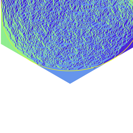
Figure 1: A limit shape simulation. The “frozen boundary” (yellow), which is asymptotically the boundary of the facets, is a cardioid.

Let $C_{n}$ be a sequence of boundary contours each of which can be spanned by at least one stepped surface; we will call such contours tilable. Suppose that $n^{-1}\,C_{n}$ converges to a given curve $C\subset\mathbb{R}^{3}$. In this case $C$ can be spanned by a Lipschitz surface whose normal (which exists almost everywhere) points into the positive octant (any limit of stepped surfaces of the $C_{n}$ is such a surface); we will call such contours $C$ feasible. It is well-known, see e.g. [6] that feasibility is equivalent to being a limit of tilable contours.

It is natural to consider the weak limit of the corresponding uniform measures on stepped surfaces of $C_{n}$, scaled by $n^{-1}$. A form of the law of large numbers, proved in [3], says that this limit depends only on the contour $C$ and is, in fact, a $\delta$-measure on a single Lipschitz surface spanning $C$. This surface, known as the limit shape, can, for example, be interpreted as the macroscopic shape of an interface (e.g. crystal surface) arising from its microscopic description and boundary conditions.

A question of obvious interest is to describe this limit shape quantitatively and qualitatively. In particular, an important phenomenon, observed in nature and reproduced in this simple model, is formation of facets, that is, flat pieces, in the limit shape.

1.3 Variational principle

The following variational characterization of the limit shape was proved in [3]. The limit shape may be parameterized as the graph of a function

$$x_{3}=h(x_{3}-x_{1},x_{3}-x_{2})$$

where $h$ is a Lipschitz function with gradient $\nabla h$ (which is defined almost everywhere by Rademacher’s theorem) in the triangle

$$\Delta=\textup{conv}\,\big{\{}(0,0),(0,1),(1,0)\big{\}}\,.$$ (1)

Let $\Omega$ be the plane region enclosed by the projection of the boundary curve $C$ along the $(1,1,1)$-direction. We will use

$$(x,y)=(x_{3}-x_{1},x_{3}-x_{2})$$

as coordinates on $\Omega$. The limit shape height function $h$ is the unique minimizer of the functional

$$\text{ENT}(h)=\int_{\Omega}\sigma(\nabla h(x,y))\,dx\,dy\to\min$$ (2)

among all Lipschitz functions with the given boundary conditions (that is, for which the graph of $h$, restricted to $\partial\Omega$, is $C$) and gradient in $\Delta$. Here $\sigma$ is the surface tension. It has an explicit form which, in the language of [13], is the Legendre dual of the Ronkin function of the simplest plane curve

$$z+w=1\,.$$

We recall that for a plane curve $P(z,w)=0$, its Ronkin function [15] is defined by

$$\mathcal{R}(x,y)=\frac{1}{(2\pi i)^{2}}\iint_{\begin{subarray}{c}|z|=e^{x}\\ |w|=e^{y}\end{subarray}}\log\big{|}P(z,w)\big{|}\,\frac{dz}{z}\,\frac{dw}{w}\,.$$

The gradient $\nabla\mathcal{R}$ always takes values in the Newton polygon $\Delta(P)$ of the polynomial $P$, so $\Delta(P)$ is naturally the domain of the Legendre transform $\sigma=\mathcal{R}^{\vee}$. For the straight line as above, the Newton polygon is evidently the triangle (1). See Figure 2.

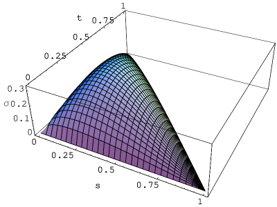
Figure 2: Graph of $-\sigma$ for the line $P(z,w)=z+w-1$.

1.4 General planar graphs

More generally, to an arbitrary planar periodic bipartite edge-weighted graph (with periodic edge weights) one associates a real plane curve $P(z,w)=0$, its spectral curve. Limit shapes for the height function in the corresponding dimer problem satisfy the same variational principle as above with $\sigma=\mathcal{R}^{\vee}$, where $\mathcal{R}$ is the Ronkin function of $P(z,w)$, see [13]. The spectral curve $P$ of the dimer model is always a so-called Harnack curve. This property, also known as maximality, is crucial for the constructions in this paper. Harnack curves form a very special class of real plane curves, see [11]. Many probabilistic implications of maximality are discussed in [13].

Maximality, in particular, implies that the surface tension $\sigma$ is analytic and strictly convex in the interior $\Delta(P)^{\circ}$ of $\Delta(P)$, with the exception of lattice points, that is, points of $\mathbb{Z}^{2}$. At a lattice point, generically, $\sigma$ has a conical singularity, often referred to as a cusp in physics literature. For example, at the point $(0,0)$ in Figure 2, $\sigma$ has the form

$$\sigma(s,t)=t\ln\frac{t}{t+s}+s\ln\frac{s}{t+s}+o(s,t)\,,$$

in which the reader will recognize the Shannon entropy. More generally, at a lattice point, the graph of $\sigma$ is approximated by a cone over a curve which is the polar dual of the curve bounding the corresponding facet of the Ronkin function. Such singularities lead to facet formation in the minimizer. They disappear only if the spectral curve has a nodal singularity, which is a codimension two condition on the weights in the dimer model.

At the boundary of the Newton polygon, $\sigma$ is piecewise-linear and, in particular, not strictly convex. This loss of strict convexity leads to edges in the limit shape. Both facets and edges are clearly visible in the simulation in Figure 1.

These features of the surface tension make the analytic study of the variational problem (2) challenging and interesting.

1.5 Complex Burgers equation

We say that a point $(x_{0},y_{0})\in\Omega$ is in the liquid region if the minimizer $h(x,y)$ is $C^{1}$ in a neighborhood of $(x_{0},y_{0})$ and $\nabla h(x_{0},y_{0})$ is either in $\Delta(P)^{\circ}\setminus\mathbb{Z}^{2}$ or at a point (in $\mathbb{Z}^{2}$) corresponding to a nodal singularity of $P$. This terminology is motivated by the frozen/liquid/gaseous classification of phases of a dimer model [13].

Since $\sigma$ is analytic and strictly convex on the liquid region, Morrey’s theorem [17] implies that $h$ is analytic there and satisfies the Euler-Lagrange equation $\operatorname{div}\nabla\sigma\circ\nabla h=0$. A more general equation

$$\operatorname{div}\nabla\sigma\circ\nabla h=c\,,$$ (3)

where $c$ is a real constant, arises in the volume-constrained minimization problem

$$\mathcal{E}(h)=\int_{\Omega}\sigma(\nabla h(x,y))\,dx\,dy+c\int_{\Omega}h(x,y)\,dx\,dy\to\min\,,$$ (4)

in which $c$ is the Lagrange multiplier for the constraint

$$\int_{\Omega}h(x,y)\,dx\,dy=\operatorname{const}$$

that forces the limit shape to enclose a given volume (or more precisely, to contain a given volume under its graph).

Our first result is the following reduction of the Euler-Lagrange equation (3) to a first-order quasilinear equation for a complex valued function $z(x,y)$.

Theorem 1.

In the liquid region, we have

$$\nabla h=\frac{1}{\pi}(\arg w,-\arg z)$$ (5)

where the functions $z$ and $w$ solve the differential equation

$$\frac{z_{x}}{z}+\frac{w_{y}}{w}=c$$ (6)

and the algebraic equation $P(z,w)=0$  .

Note that in (5) the argument of a complex number is a multivalued function and the statement is that there exists a branch of the argument for which equality (5) is satisfied.

For example, in the lozenge tiling case

$$P(z,w)=z+w-1$$ (7)

and without the volume constraint, equation (6) becomes

$$\frac{z_{x}}{z_{y}}=\frac{z}{1-z}$$

which becomes the standard complex inviscid Burgers equation

$$u_{x}=uu_{y}$$ (8)

upon the substitution $u=z/(1-z)$. In general, equation (6), being a first-order quasilinear equation for $z(x,y)$, has properties parallel to those of (8) and, in particular, it can be solved by complex characteristics as follows:

Corollary 1.

For $c\neq 0$ there exists an analytic function $Q$ of two variables such that

$$Q(e^{-cx}z,e^{-cy}w)=0$$

in the liquid region. When $c=0$ there is an analytic function $Q_{0}$ of two variables such that

$$Q_{0}(z,w)=xzP_{z}+ywP_{w}.$$ (9)

In other words (for $c\neq 0$), as functions of $x$ and $y$, $z$ and $w$ are found by solving the system

$$\begin{cases}P(z,w)=0\,,\\ Q(e^{-cx}z,e^{-cy}w)=0\,.\end{cases}$$ (10)

A general solution to the Euler-Lagrange equation (3) is thus parameterized by an analytic curve $Q=0$ in the plane.

Below we define a dense set of boundary conditions for which $Q$ is in fact algebraic. In this case (10) is a system of algebraic equations and, hence, $h$ is an integral of an algebraic function of $e^{-cx}$ and $e^{-cy}$.

1.6 Frozen boundary

The liquid region may extend all the way to the boundary of $\Omega$, but it may happen that it ends at a facet, that is, a domain where the limit shape height function $h$ is a linear function with integral gradient, as in Figure 1. We call the boundary between the liquid region and the facets the frozen boundary.

There are two kinds of facets: the ones with gradient $\nabla h$ in the interior of the Newton polygon $\Delta(P)$ and the ones with $\nabla h$ on the boundary of $\Delta(P)$. While the corresponding microscopic properties of random surfaces are, in a sense, diametrically opposite (they correspond to gaseous and frozen phases, respectively, in the classification of [13]), the only difference relevant for this paper is that only gaseous facets can occur in the interior of the domain. We will call such floating facets bubbles.

In terms of (5), a point $(z,w)$ of the frozen boundary is a real point of the spectral curve $P(z,w)=0$. A curve’s worth of such real solutions of (10) is possible only if $Q$ is real. In this case, at the frozen boundary, the solutions $(z,w)$ and $(\bar{z},\bar{w})$ of the system (10) become identical. That is, the frozen boundary is a shock for the equation (6). In contrast to the usual real-valued Burgers equation, a shock is a special event in the complex case as complex characteristics tend to miss each other.

Given two analytic functions $P$ and $Q$, the locus where the system (10) has a double root is itself an analytic curve in the $(x,y)$-plane. In the case when $P$ and $Q$ are algebraic, this discriminant curve is of the form

$$\tilde{R}(e^{-cx},e^{-cy})=0\,,$$ (11)

where $\tilde{R}$ is polynomial which can be written down effectively in terms of resultants.

The frozen boundary $R$ is a subset (in principle, proper) of the discriminant curve (11). A more invariant way of saying the same thing is that the map

$$\operatorname{\mathcal{E}xp}:(x_{1},x_{2},x_{3})\mapsto\left(e^{cx_{1}}:e^{cx_{2}}:e^{cx_{3}}\right)\in\mathbb{R}\mathbf{P}^{2}$$

from $\mathbb{R}^{3}$ to the real projective plane takes the frozen boundary to a real algebraic curve. As $c\to 0$ the map $\operatorname{\mathcal{E}xp}$, suitably rescaled, becomes the projection in the $(1,1,1)$ direction. Monotonicity insures that our random surfaces are mapped 1:1 by $\operatorname{\mathcal{E}xp}$. Indeed, if $(x_{1},x_{2},x_{3})$ is on the surface then $(x_{1}+t,x_{2}+t,x_{3}+t)$ is on the surface only for $t=0$.

At a generic point, the frozen boundary is smooth and (10) has exactly one real double root. The functions $z(x,y)$ and $w(x,y)$ have a square-root singularity at the frozen boundary and, hence, the arguments of $z$ and $w$ grow like the square root of the distance as one moves from the frozen boundary inside the liquid region. Integrating (5), we conclude that the limit shape height function has an $x^{3/2}$ singularity at the frozen boundary. Thus one recovers the well-known Pokrovsky-Talapov law [21] in this situation.

At special points of the frozen boundary, triple solutions of (10) occur. At such points, the frozen boundary has a cusp singularity. One such point can be seen in Figure 1.

1.7 Algebraic solutions

Any boundary contour can be approximated by piecewise linear contours and even by piecewise linear contours $C$ with segments in coordinate directions. For such contours the function $Q$ is algebraic (of degree growing with the number of segments). In this paper we will prove this in the simplest case when $P(z,w)=z+w-1$ and the boundary $C$ is connected. The precise result that we will prove is the following

Theorem 2.

Suppose $P(z,w)=z+w-1$ and the boundary contour $C$ is feasible, connected, and polygonal with $3d$ sides in coordinate directions (cyclically repeated). Then $Q$ is an algebraic curve of degree $d$ and genus zero.

The corresponding result for cases in which some of the edge lengths are allowed to be zero can be obtained as limits, letting the edge lengths shrink. In these cases $Q$ may have smaller degree.

1.8 Reconstruction of limit shape from the Burgers equation

The frozen boundary $R$ is a genus zero curve inscribed in the polygon $\operatorname{\mathcal{E}xp}(C)$. The reconstruction of the limit shape from $R$ has the following elementary geometric interpretation.

Let $\mathbf{x}=(x_{1},x_{2},x_{3})$ be a point on the limit shape in the liquid region. Then $\operatorname{\mathcal{E}xp}(\mathbf{x})$ lies inside the frozen boundary $R$. In the course of proving Theorem 2, we will show that there is a unique, up to conjugation, complex tangent to $R$ through the point $\operatorname{\mathcal{E}xp}(\mathbf{x})$. This is illustrated in the Figure 3. There are 3 tangent lines to a cardioid through a general point in the plane (this number of tangents is the degree of the dual curve and is classically known as the class of a curve). Through a point outside the cardioid, all 3 of these lines are real. Through a point inside the cardioid, only one real tangent exists, the other two tangents are complex.

Figure 3: Tangent lines to a cardioid

Let the complex tangent through $\operatorname{\mathcal{E}xp}(\mathbf{x})$ be given by the equation

$$a_{1}z_{1}+a_{2}z_{2}+a_{3}z_{3}=0$$

in homogeneous coordinates $(z_{1}:z_{2}:z_{3})$ on the projective plane. Since the point $\operatorname{\mathcal{E}xp}(\mathbf{x})$ lies on this line, this gives us a triangle in the complex plane illustrated in Figure 4.

Figure 4: A complex tangent defines a triangle

The numbers $(a_{1},a_{2},a_{3})$ are unique up to common complex factor and complex conjugation. If follows that the similarity class of the triangle in Figure 4 is well defined, in particular, its angles $\alpha_{1},\alpha_{2},\alpha_{3}$ are well defined. Formula (5) simply says that

$$(\alpha_{1},\alpha_{2},\alpha_{3})\in\mathbb{R}_{>0}^{3}$$

is the normal to the limit shape at the point $\mathbf{x}$.

As the point $\mathbf{x}$ approaches the frozen boundary, the complex tangent approaches the corresponding real tangent, the triangle degenerates, and the normal starts pointing in one of the coordinate directions.

Higher genus frozen boundaries occur for multiply connected liquid regions. The holes may be created manually by considering surfaces spanning a disconnected boundary contour or they may appear as bubbles for spectral curves $P$ of genus $\geq 1$. Examples of such situations will be considered in Sections 5.1 and 5.2. In the multiply-connected case, the Burgers equation needs to be supplemented by period conditions, see Sections 2.5.

1.9 Burgers equation in random matrix theory

In the case when $\Omega$ is an infinite vertical strip, the random surface model studied here can be conveniently restated in terms of nonintersecting lattice paths connecting given points on $\partial\Omega$. The continuous limit of such nonintersecting path models is well-known to be described by the Hermitian $2$-matrix model (in other words, by a random walk on the space of Hermitian matrices with boundary conditions in given conjugacy classes). In physics literature, complex Burgers equation first appeared in this context in the work of Matytsin [14]. Its rigorous mathematical study appears in the work of A. Guionnet [5]. Generalizations of these equations to interacting particle systems are discussed in [1].

1.10 Acknowledgments

The paper was started during the authors’ visit to Institut Henri Poincaré in the Spring of 2003. The work was continued while R.K. was visiting Princeton University. We thank these institutions for their hospitality.

The work of R.K. was partially supported by CNRS and NSERC. A.O. was partially supported by the NSF and a fellowship from the Packard Foundation.

We benefited from discussions with A. Abanov, A. Guionnet, N. Reshetikhin, I. Rodnianski, S. Sheffield, and S. Smirnov.

2 Complex Burgers equation

2.1 Proof of Theorem 1

By the basic properties of the Ronkin function, see [15], the function

$$\nabla\sigma=(\nabla\mathcal{R})^{-1}:\mathbb{R}^{2}\to\mathbb{R}^{2}$$

takes values in the amoeba of the spectral curve. By definition, this means that for any $(x,y)$ in the liquid region we can find a point $(z,w)$ on the spectral curve satisfying

$$\big{[}\nabla\sigma\circ\nabla h\big{]}(x,y)=(\log|z|,\log|w|)\,.$$ (12)

By our hypothesis, near $(x,y)$ the LHS of (12) lies in the interior of the amoeba. One of the several equivalent definitions of a Harnack curve is that the map

$$(z,w)\mapsto(\log|z|,\log|w|)$$ (13)

from the curve to its amoeba is 2-to-1 with nonzero Jacobian over the amoeba’s interior. Therefore, the lift $(x,y)\mapsto(z,w)$ in (12) is unique up to complex conjugation, and real analytic in a neighborhood of $(x_{0},y_{0})$.

Using (12), the Euler-Lagrange equation (3) stated in terms of $(z,w)$ becomes

$$\Re\left(\frac{z_{x}}{z}+\frac{w_{y}}{w}\right)=c\,,$$

This first order equation for the gradient $\nabla h$ needs to be supplemented by the usual consistency relation for the mixed partials:

$$\left(-\frac{\partial}{\partial y},\frac{\partial}{\partial x}\right)\cdot\nabla h=\left(-\frac{\partial}{\partial y},\frac{\partial}{\partial x}\right)\cdot\nabla\mathcal{R}\,(\log|z|,\log|w|)=0\,.$$ (14)

Again, it is a special property of the Harnack curve that

$$\nabla\mathcal{R}\,(\log|z|,\log|w|)=\frac{1}{\pi}\left(\mp\arg w,\pm\arg z\right)$$ (15)

where on the right we mean a lift of $(\mp\arg w,\pm\arg z)$ and where the choice of signs depends on the choice of one of the preimages in (13), see [20] and also [15]. This turns the relation (14) into the imaginary part of (6) (since $c\in\mathbb{R}$) and concludes the proof.

2.2 Proof of Corollary 1

Since $z$ and $w$ satisfy an algebraic equation $P(z,w)=0$, their Jacobian vanishes

$$J(z,w)=\det\begin{pmatrix}z_{x}&z_{y}\\ w_{x}&w_{y}\end{pmatrix}=0\,.$$

We have

$$J(e^{-cx}z,e^{-cy}w)-J(z,w)=c^{2}zw-czw_{y}-cz_{x}w=0$$

by (6) and hence $J(e^{-cx}z,e^{-cy}w)=0$ identically. The functions $e^{-cx}z$ and $e^{-cy}w$ are real analytic in the liquid region and the vanishing of the Jacobian implies a functional dependence of the form

$$Q(e^{-cx}z,e^{-cy}w)=0\,,$$

where $Q$ is an analytic function (note that if $W=W(x,y),Z=Z(x,y)$ satisfy $Z_{x}W_{y}=Z_{y}W_{x}$, then $\partial W/\partial\bar{Z}=W_{x}/Z_{x}-W_{y}/Z_{y}=0$, so that $W$ is an analytic function of $Z$, and vice versa.)

2.3 Complex structure on the liquid region

Consider the function

$$\zeta=e^{-cx}z$$

which is defined on the liquid region. Differentiating $P(z,w)$ with respect to $y$ and using (6) implies that

$$\frac{\zeta_{x}}{\zeta_{y}}=\frac{zP_{z}}{wP_{w}}$$ (16)

when $P(z,w)=0$. The rational function

$$(z,w)\mapsto\gamma(z)=\frac{zP_{z}}{wP_{w}}\in\mathbb{C}\mathbf{P}^{1}$$

is known as the logarithmic Gauß map of the spectral curve $P(z,w)=0$.

By a result of Mikhalkin [15], the preimage $\gamma^{-1}\left(\mathbb{R}\mathbf{P}^{1}\right)$ is precisely the critical locus of the map from the curve to its amoeba. For a Harnack curve, therefore, it coincides with the real locus. It follows that on the liquid region $\gamma$ takes values in upper or lower half-plane, depending on the choice of lift of (12). With one of the choices, the map

$$(x,y)\to\zeta$$

is orientation-preserving and we can use it to pull back the complex structure.

Note that one could equally well take the function $e^{-cy}w$ as defining the complex structure on the liquid region. However, by Corollary 1 the complex structure thus obtained is the same. Yet another way to say this is that

$$(x,y)\mapsto(e^{-cx}z,e^{-cy}w)$$

maps the liquid region to the analytic curve $Q=0$ and the complex structure on the liquid region is the unique one making this map holomorphic.

The orientation-preserving property of $\zeta(x,y)$ can be strengthened as follows

Proposition 2.

For $c\neq 0$ and $(x,y)$ in the liquid region, the map

$$\pi_{Q}:(x,y)\mapsto(e^{-cx}z,e^{-cy}w)\in Q$$ (17)

is an orientation preserving local diffeomorphism onto its image. In the case $P(z,w)=z+w-1$ the map is a diffeomorphism onto its image.

Proof.

Suppose that $\pi_{Q}$ maps two distinct points $(x_{1},y_{1})$ and $(x_{2},y_{2})$ to the same point

$$(e^{-cx_{1}}z_{1},e^{-cy_{1}}w_{1})=(e^{-cx_{2}}z_{2},e^{-cy_{2}}w_{2})\in Q$$

of $Q$, where $z_{i}=z(x_{i},y_{i})$. This means that on the curve $P$ we have a pair of distinct points

$$P\owns(z_{1},w_{1})\neq(z_{2},w_{2})\in P$$

with the same arguments

$$\arg(z_{1},w_{1})=\arg(z_{2},w_{2})\,.$$

However, $P$ is a Harnack curve and for a such a curve we have (15). By strict convexity of the Ronkin function, its gradient maps both components of $P(\mathbb{C})\setminus P(\mathbb{R})$ one-to-one to the Newton polygon of $P$, and, as a result, a point of $P$ is locally determined by the arguments. If $P=z+w-1$ (or even if $P$ has degree $\leq 2$), a point of $P$ in a component of $P(\mathbb{C})\setminus P(\mathbb{R})$ is determined uniquely by its arguments. ∎

There are examples where $\pi_{Q}$ is a non-trivial covering map.

In the case $c=0$, we can use $z$ or $w$ to define the complex structure. This complex structure is used in [10] in the study of the fluctuations of the random surfaces. Conjecturally, the Gaussian correction to the limit shape is given by the massless free field in the conformal structure defined by $\zeta$.

2.4 Genus of $Q$

Suppose that the liquid region is surrounded by the frozen boundary, that is, suppose that $\Im z,\Im w\to 0$ at the boundary of the liquid region. The real parts $\Re z$ and $\Re w$ may or may not be continuous at the boundary of the liquid region.

Proposition 3.

If the liquid region is surrounded by the frozen boundary and the functions $z(x,y)$ and $w(x,y)$ are continuous up to the frozen boundary then the curve $Q$ is algebraic. If $P=z+w-1$ then $Q$ is of the same genus as the liquid region.

Proof.

If $z,w$ are continuous then the map (17), and its complex conjugate glue along the boundary of the liquid region to a map from the double of the liquid region to the curve $Q$. This map is orientation preserving and unramified by Proposition 2, and so a covering map of $Q$. It follows that the analytic curve $Q$ is compact. If $P=z+w-1$, the map is a diffeomorphism and therefore $Q$ is of the same genus as the liquid region. ∎

Conversely, if $Q$ is algebraic then the solutions of (10) are continuous. However, only for some very special curves $Q$ will the solution of (10) satisfy the global requirements of being single-valued in some region and becoming real at the region’s boundary.

By taking limits of algebraic solutions, one can construct solutions having, for example, accumulation points of cusps. At such a point $z$ is discontinuous. Namely, $z$ turns infinitely many times around $\mathbb{R}\mathbf{P}^{1}$ as one approaches the accumulation point along the frozen boundary.

It would be interesting to prove the continuity required in Proposition 3 directly from the variational problem and polygonality of the boundary conditions. In this paper, we take a different route and construct the algebraic curve $Q$ by a deformation argument.

Note that Proposition 3 forces $Q$ to have the maximal possible number of real ovals (real components), namely genus plus one. Such real curves are known as $M$-curves.

2.5 Islands and bubbles

Holes in the liquid region may arise by considering surfaces spanning a disconnected boundary contour or they may appear as gaseous bubbles (where the surface tension has a cusp). We will call such holes islands and bubbles, respectively. A schematic representation of an island and a bubble can be seen in Figure 5

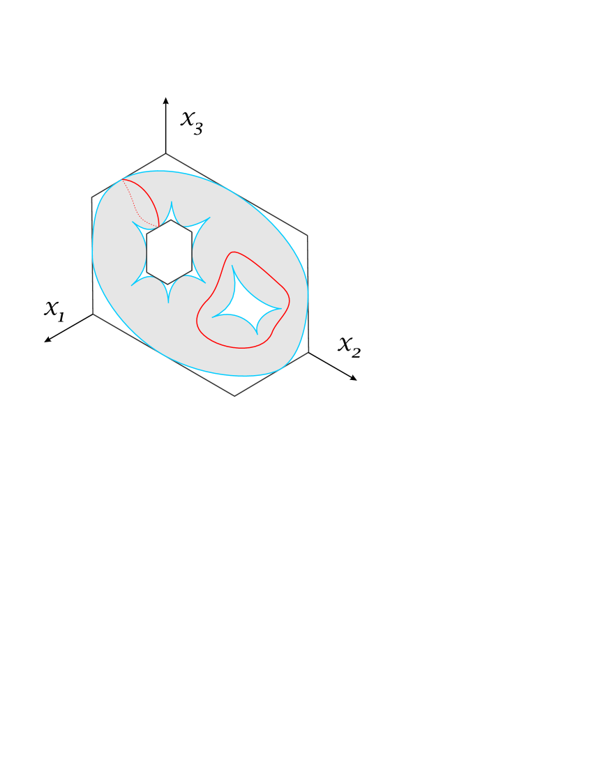
Figure 5: An island, a bubble, and their period conditions.

In principle, the solutions of a system like (10) may pick up a monodromy around a nontrivial loop in the liquid region. However, in our case we require them to be single-valued because they are determined by the single-valued function $\nabla h$.

In the presence of holes, the Burgers equation (6) needs to be supplement by integral constraints. This constraints can be phrased as imposing conditions on the periods of the curve $Q$.

2.5.1 Areas of bubbles

In the case of a bubble inside the liquid region, it is more convenient to use the integrated form of (3) which says that the flow of the vector field $\nabla\sigma\circ\nabla h$ through any closed contour equals $c$ times the area enclosed.

Let a domain $B\subset\Omega$ be such that its boundary $\partial B$ is smooth and lies in the liquid region. Consider a variation of $h$ which is a smooth approximation to the characteristic function of $B$. This yields the real part of the equation

$$\int_{\partial B}\alpha=c\,\operatorname{Area}(B)\,.$$ (18)

where $\alpha$ is the following $1$-form

$$\alpha=\log z\,dy-\log w\,dx\,.$$

By (5), the vanishing of the imaginary part of (18) means that the height function $h$ is well-defined. Thus (18) is satisfied by any $B$ as above.

Suppose that $(z,w)$ are continuous up to the frozen boundary. On the frozen boundary, the points $(e^{-cx}z,e^{-cy}w)$ and $(z,w)$ are real points of $Q$ and $P$, respectively. This allows us to associate, to each oval of $Q$, a corresponding oval of $P$. We will call an oval compact if it does not intersect the coordinate axes. Note that an oval of $Q$ is compact if and only if the corresponding oval of $P$ is. Because $P$ is a Harnack curve, it has exactly one noncompact oval that intersects each coordinate axis $\deg P$ times.

If $B$ is a bubble, a point on its boundary gives a point $(z,w)\in P$ belonging to a compact oval of $P$. Integrating (18) around the boundary of $B$, the imaginary part of the left-hand side of (18) is then zero, since on the boundary of a bubble $z$ and $w$ are real and of definite sign. However the real part may not vanish and represents a nontrivial constraint of the curve $Q$. This constraint can be reformulated as follows.

Given a compact oval $O$ of an plane curve, consider its logarithmic area

$$\operatorname{LogArea}(O)=\int_{O}\log z\,d\log w\,,$$

that is, the area enclosed by the image of $O$ under the amoeba map.

Proposition 4.

The logarithmic areas of compact ovals of $Q$ are multiples of the logarithmic areas of the corresponding ovals of $P$. The multiple at a given oval is given by the winding number of the map from the corresponding bubble $B$ to the oval of $Q$.

Proof.

Let $O_{P}$ and $O_{Q}$ be the ovals of $P$ and $Q$ corresponding to a bubble $B$. Because these ovals are compact, the logarithms of $z$, $w$, $\zeta=e^{-cx}z$ and $\omega=e^{-cy}w$ are well-defined on $\partial B$. We have

$$\operatorname{LogArea}(O_{Q})=\int_{\partial B}\log\zeta\,d\log\omega=\\ c^{2}\int_{\partial B}x\,dy-c\int_{\partial B}(y\,d\log z+x\,d\log w)+\int_{\partial B}\log z\,d\log w=\\ c^{2}\operatorname{Area}(B)-c\int_{\partial B}\alpha+m\operatorname{LogArea}(O_{P})=m\operatorname{LogArea}(O_{P})\,,$$

where $m$ is the winding number of $\partial B$ around $O_{Q}$. ∎

2.5.2 Heights of islands

Different period conditions need to be imposed if $\Omega$ has interior boundary as in Figure 5 or in the example considered in Section 5.1. In this case, $z$ and $w$ take values on the big oval of the spectral curve and do change sign on $\partial B$. In this case, the vanishing of the imaginary part of (18) is equivalent to the condition that the polygon inscribed in $B$ lifts to a closed contour in $\mathbb{R}^{3}$, see the discussion after the statement of Theorem 3 below. The argument that was used to derive the real part of (18) is no longer valid and, in fact, the real part of (18) no longer holds. Instead, we have a different period condition that fixes the relative height of the island with respect to other components of $\partial\Omega$.

Let $\partial\Omega_{1}$ be the component of $\partial\Omega$ around which our island forms. Let $\partial\Omega_{0}$ be a different component of $\partial\Omega$ which respect to which the height of the island will be measured. Equation (5) implies that

$$dh=-\frac{1}{\pi}\,\Im\alpha,$$

and hence

$$\textup{height}\left(\partial\Omega_{1}\right)-\textup{height}\left(\partial\Omega_{0}\right)=\frac{1}{\pi}\Im\int_{\partial\Omega_{1}}^{\partial\Omega_{0}}\alpha\,,$$

where the integration is along a path connecting the two boundaries as in Figure 5.

For contour as in Figure 5, at the endpoints we have $z=0$ and $w\in\mathbb{R}\setminus 0$. In particular, the forms $\log z\,d\log w$ and $\log\zeta\,d\log\omega$ are integrable near the corresponding points of $P$ and $Q$. The same computation as in proof of Proposition 4 shows that

$$\textup{height}\left(\partial\Omega_{1}\right)-\textup{height}\left(\partial\Omega_{0}\right)=\frac{1}{c\pi}\Im\int_{\partial\Omega_{0}}^{\partial\Omega_{1}}\log\zeta\,d\log\omega+\textup{const}\,.$$ (19)

The path of the integration in (19) connects the points of intersection of two different real ovals of $Q$ with the line $z=0$. We will call it the height of one oval with respect to another.

In Section 3.1.4, we will show that the logarithmic areas of compact ovals of $Q$, the heights of the noncompact ovals, and the points of intersection of $Q$ with the coordinate axes can be chosen as local coordinates on the space of nodal plane curves of given degree and genus. This suggests constructing the required curve $Q$ by deformation from the equally weighted, no islands case treated in the present paper. We hope to address this in a future paper.

3 Proof of theorem 2

3.1 Winding curves and cloud curves

3.1.1 Winding curves

As we will see, the rational curve $Q$ in the statement of Theorem 2 is not just any rational plane curve, it has some very special properties. We begin the proof of Theorem 2 with a discussion of these special properties.

We say that a degree $d$ real algebraic curve $C\subset\mathbb{R}\mathbf{P}^{2}$ is winding if

1. it intersects every line $L\subset\mathbb{R}\mathbf{P}^{2}$ in at least $d-2$ points counting multiplicity, and

2. there exists a point $p_{0}\in\mathbb{R}\mathbf{P}^{2}\setminus C$ called the center, such that every line through $p_{0}$ intersects $C$ in $d$ points.

The center $p_{0}$ in the above definition is obviously not unique: any point sufficiently close to $p_{0}$ can serve as a center instead. The existence of a center implies that every winding curve is hyperbolic, that is, it lies in the closure of the set of curves having $[d/2]$ nested ovals encircling the center. Much is known about hyperbolic curves, see e.g. [22, 23].

Winding curves are almost never smooth. They typically have nodes, but may also have ordinary triple, quadruple etc., points as well as tacnodes (points where two branches are tangent). This, however, exhausts the list of possible singularities in view of the following

Proposition 5.

All singularities of a winding curve $C$ are real. Every branch of $C$ through a singularity is real, smooth, and has contact of order $\leq 3$ with its tangent, that is, it has at most ordinary flexes. The only double tangents of a winding curve are ordinary tacnodes with two branches on the opposite sides of the common tangent.

Proof.

Let $p$ be a complex singularity of $C$. The line joining $p$ with the complex conjugate point $\bar{p}$ is real and meets $C$ in at least $4$ complex points counting multiplicity—contradicting the definition. Similarly, a complex branch through a singularity yields complex intersection points with any line that just misses the singularity, in contradiction with part (2) of the definition.

Now suppose the origin is a real singularity of $C$ and let a branch of $C$ be parameterized by

$$x=t^{a}\,,\quad y=t^{b}+\dots\,,$$

where $a<b$. The line $y=0$ meets this branch with multiplicity $b$ whereas the nearby line $y=\epsilon$ meets it in $1$ real point if $b$ is odd and may miss it entirely if $b$ is even. It follows that $b\leq 3$.

The case $(a,b)=(2,3)$ of an ordinary cusp is ruled out by considering a line from the cusp to the center $p$. The order of contact with a nearby line through $p$ will drop by $2$.

It is easy to see that a line that is tangent to two distinct points of $C$ can be moved so that it loses $4$ real points of contact. The same is true if two branches of $C$ are on the same side of the common tangent, or tangent at a flex (in which case the multiplicity of the intersection with the tangent line is at least four greater than for that of certain nearby lines). ∎

3.1.2 Moduli of rational winding curves

It follows from Proposition 5 that a winding curve $Q$ is always immersed, that is, the map

$$f:\widetilde{Q}\to\mathbf{P}^{2}$$ (20)

from the normalization of $Q$ to the plane is an immersion. In this paper, we will focus on the winding curves of genus zero, in which case $\widetilde{Q}\cong\mathbf{P}^{1}$.

Clearly, if $Q$ is irreducible, winding, and without tacnodes, then all small deformations of the map (20) remain winding. In other words, such curves form an open set of the real locus of the moduli space $\mathcal{M}_{0}(\mathbf{P}^{2},d)$ of degree $d$ maps

$$f:\mathbf{P}^{1}\to\mathbf{P}^{2}$$

considered up to a reparameterization of the domain. This moduli space is smooth of dimension $3d-1$, see [7]. This is because the projective plane $\mathbf{P}^{2}$ is convex, which, by definition, means that its tangent bundle is generated by global sections (concretely, the vector fields generating the $SL(2)$-action span the tangent space to $\mathbf{P}^{2}$ at any point). The tangent space to $\mathcal{M}_{0}(\mathbf{P}^{2},d)$ at the point $Q$ may be identified with the global sections $H^{0}(N_{\mathbf{P}^{2}/Q})$, where $N_{\mathbf{P}^{2}/Q}$ is the normal bundle (it is a bundle because $Q$ is immersed).

Suppose that the Newton polygon of $Q$ is nondegenerate, that is, suppose that $Q$ does not pass through the intersections of coordinate axes in $\mathbf{P}^{2}$. Consider the monomials in $Q(z,w)=0$ on the boundary of the Newton polygon. This gives $3d$ numbers modulo overall scale, matching the dimension $3d-1$ of the moduli space. These outside monomials determine the $3d$ intersections of $Q$ with coordinate axes. In fact, these intersections should be properly considered as a point in $(S^{d}\,\mathbb{C}^{*})^{3}$, subject to one constraint, which precisely identifies it with the outside coefficients of $Q(z,w)$.

Proposition 6.

The outside coefficients of $Q(z,w)$ are local coordinates on $\mathcal{M}_{0}(\mathbf{P}^{2},d)$ near an immersed curve $Q$ with a nondegenerate Newton polygon.

Proof.

Let $\xi$ be a nonzero section of the normal bundle $N_{\mathbf{P}^{2}/Q}$. Let some branch of $Q$ intersect the axis $w=0$ at the point $(z_{0},0)$ with multiplicity $m$. This intersection is preserved by $\xi$ if and only if $\xi$ vanishes at $(z_{0},0)$ with the same order $m$. The differential

$$\eta=f^{*}(\iota_{\xi}\,d\log z\wedge d\log w)$$ (21)

is a well-defined nonzero meromorphic differential on $\mathbf{P}^{1}$. One checks that, in fact, it is everywhere regular. Indeed, near $(z_{0},0)$ we have

$$w=a(z-z_{0})^{m}+\dots\,,\quad\xi=b(z-z_{0})^{m}\,\frac{d}{dw}+\dots$$

where $a\neq 0$ and dots stand for $o((z-z_{0})^{m})$. Thus

$$\eta=-\frac{b}{az}\,dz+\dots$$

and we have produced a nonzero regular differential on a genus $0$ curve, a contradiction. ∎

Three types of degeneration can happen to $Q$ in codimension one, see e.g. [8]. It can develop either:

1. a cusp, or

2. a tacnode, or

3. an extra node, and, hence, become reducible.

All these degenerations mark the boundary of the winding locus in $\mathcal{M}_{0}(\mathbf{P}^{2},d)$. By Proposition 5, a cusp can develop only when a loop of $Q$ ties tight around the center $p$, as, for example, for

$$Q=z^{2}-(w-\epsilon)^{2}(w+\epsilon)\,,\quad p=(0,0)\,,\quad\epsilon\to 0\,.$$

In this case, the frozen boundary, which is the dual curve of $Q$, escapes to infinity and so this case will not concern us in the present paper.

Curves with a tacnode or an extra node form codimension $1$ boundary strata of the winding locus. A real tacnode can deform to a pair of real nodes or a pair of complex nodes; only in the first case does the curve remain winding. Similarly, only one of the two smoothings of the new node is winding.

3.1.3 Cloud curves

The dual curve $C^{\vee}$ of a winding curve $C$ separates the dual projective plane into the regions formed by those lines that intersect $C$ in $d$ and $d-2$ points. We will call them the exterior and the interior of $C^{\vee}$, respectively. The line corresponding to the pencil of lines though the center $p$ lies entirely in the exterior of $C^{\vee}$. By making it the line at infinity, the curve $C^{\vee}$ is placed into the affine plane $\mathbb{R}^{2}$.

Since $C$ has no cusps, $C^{\vee}$ has no inflection points and, hence, is locally convex except for cusps. The cusps point into the interior of $C^{\vee}$, which makes the interior of $C^{\vee}$ resemble in shape a cloud, see Figure 16. This is why we call the dual of a winding curve a cloud curve. Node that a cloud curve has no real nodes other than tacnodes, for they would correspond to double tangents to $C$.

By construction, a cloud curve has a unique, up to complex conjugation, complex (non-real) tangent through any point in its interior.

3.1.4 Higher genus

Suppose that $Q$ is nodal curve of genus $g>0$ of the kind considered in Section 2.5, not necessarily winding. The space of nodal plane curves of given degree $d$ and genus $g$ is well known to be smooth of dimension $3d-1+g$, see [8]. As in Section 3.1.2 above, the intersections with coordinate axes give $3d-1$ degrees of freedom. The remaining $g$ dimensions come precisely from the $g$-dimensional space of holomorphic differentials as in the proof of Proposition 6.

Proposition 7.

The points of intersection with coordinate axes, the logarithmic areas of compact ovals, and the heights of the noncompact ovals, can be chosen as local coordinates at $Q$ on the moduli space of genus $g$ degree $d$ nodal plane curves.

Proof.

Consider the tangent space at $Q$ to the space of all genus $g$ curves with the same outside coefficients as $Q$. The proof of Proposition 6 identifies this tangent space with the space of regular differentials $\eta$ on the curve $Q$. Moreover, by (21), the derivative of the logarithmic area (resp. height) of an oval $O_{i}$ of $Q$ in the direction of $\eta$ is given by the real (resp. imaginary) part of $\int\eta$ along the corresponding path $\beta_{i}$ in Figure 5.

The contours corresponding to the compact ovals of $Q$ are closed and invariant under complex conjugation. Thus the corresponding periods are automatically real. As to the contours corresponding to the noncompact ovals, we can make them closed by taking their union with the complex conjugate contour (the dashed line in Figure 5). This makes the contour anti-invariant with respect to complex conjugation and thus picks out precisely the imaginary part of the original integral. Finally, since the contours in Figure 5 are disjoint, the period matrix $\int_{\beta_{i}}\eta_{j}$ is nondegenerate. ∎

3.2 Inscribing cloud curves in polygons

Let $\Omega$ is a polygon in the plane, not necessarily convex, formed by $3d$ segments with slopes $0,1,\infty$, cyclically repeated as we follow the boundary in the counterclockwise direction. Here $d=2,3,\dots$. For any constant $c$, the image of $\Omega$ under the map

$$\operatorname{\mathcal{E}xp}:(x,y)\to(e^{cx},e^{cy})$$

is a polygon in first quadrant $\mathbb{R}_{\geq 0}^{2}$. The sides of $\operatorname{\mathcal{E}xp}(\Omega)$ are formed by lines passing through the vertices of $\mathbb{R}_{\geq 0}^{2}\subset\mathbb{R}\mathbf{P}^{2}$.

We will say that a real algebraic curve $R$ is inscribed in the polygon $\operatorname{\mathcal{E}xp}(\Omega)$ if $R$ is a simple closed curve contained in $\Omega$ and tangent to lines forming the sides of $\Omega$ in their natural order. Note that near a nonconvex corner, an inscribed curve may be tangent to the line forming a side of $\Omega$ but not to the side itself.

Recall that, by definition, the class of a curve is the degree of the dual curve. Our main result in this section is the following

Theorem 3.

Let $\Omega$ be a polygon as above. A class $d$ rational cloud curve can be inscribed in $\operatorname{\mathcal{E}xp}(\Omega)$ if and only if $\Omega$ is feasible. If it exists, the inscribed curve $R$ is unique.

The tangent vector to $R$ rotates $d$ times as we go once around the curve. It follows that $R$ has $d-2$ real cusps, or one cusp per each non-convex corner of $\Omega$. Plücker formulas, see e.g. page 280 of [4], imply that the degree of $R$ equals $2d-2$. In absence of tacnodes, in addition to the $d-2$ real cusps, the curve $R$ has $2d-4$ complex cusps and $2(d-2)(d-3)$ complex nodes.

The curve $R$ being tangent to $3d$ lines imposes $3d$ incidence conditions on the degree $d$ dual curve $Q=R^{\vee}$. As discussed earlier, one of these conditions is redundant. In fact, this redundancy translates geometrically into the condition that $\Omega$ is the projection of a closed contour in $\mathbb{R}^{3}$. To see this, note that the condition of being a closed contour is equivalent to the condition that, as the boundary of $\Omega$ is traversed, the total signed displacement along each of the three edge directions is zero. If the vertical edges are at coordinates $x=x_{1},\dots,x_{d}$, the horizontal edges are at $y=y_{1},y_{2},\dots,y_{d}$ and the slope-$1$ edges are at $x-y=z_{1},z_{2},\dots,z_{d}$, then the displacements along horizontal edges are $y_{1}+z_{1}-x_{1},y_{2}+z_{2}-x_{2},\dots,y_{d}+z_{d}-x_{d}$. To be closed the sum of these displacements must be zero. The fact that the displacements in the other two directions are zero gives an identical relation. The equation

$$\sum_{i=1}^{d}y_{i}+z_{i}-x_{i}=0$$

is the logarithm of the condition that the intersection points of a plane curve with the three coordinate axes has product $1$.

Also note that while imposing $3d-1$ incidence conditions on a rational plane curve of degree $d$ gives generically a finite set of possibilities, the number of possibilities grows very rapidly. For example, there are 26312976 rational curves of degree 6 through 17 general points in the plane (all of these numbers were first determined by Kontsevich, see e.g. [7]). This shows that solving the incidence equation requires some care. In fact, our existence proof can be turned into a practical numerical homotopy procedure for finding the unique inscribed curve.

3.3 Proof of Theorem 3

3.3.1 Strategy

Our strategy will be deformation to $c\to\pm\infty$ limit, in which tropical algebraic geometry takes over. This is essentially the patchworking method of O. Viro, see e.g. [9]. A closely related approach was employed, for example, in [16] to construct curves of given degree and genus passing through given points in the plane.

From the point of view of random surfaces, letting $c\to\pm\infty$ means imposing an extreme volume constraint. As $c\to+\infty$, the limit shape becomes the unique piecewise linear surface that minimizes the volume enclosed, see an example in Figure 6.

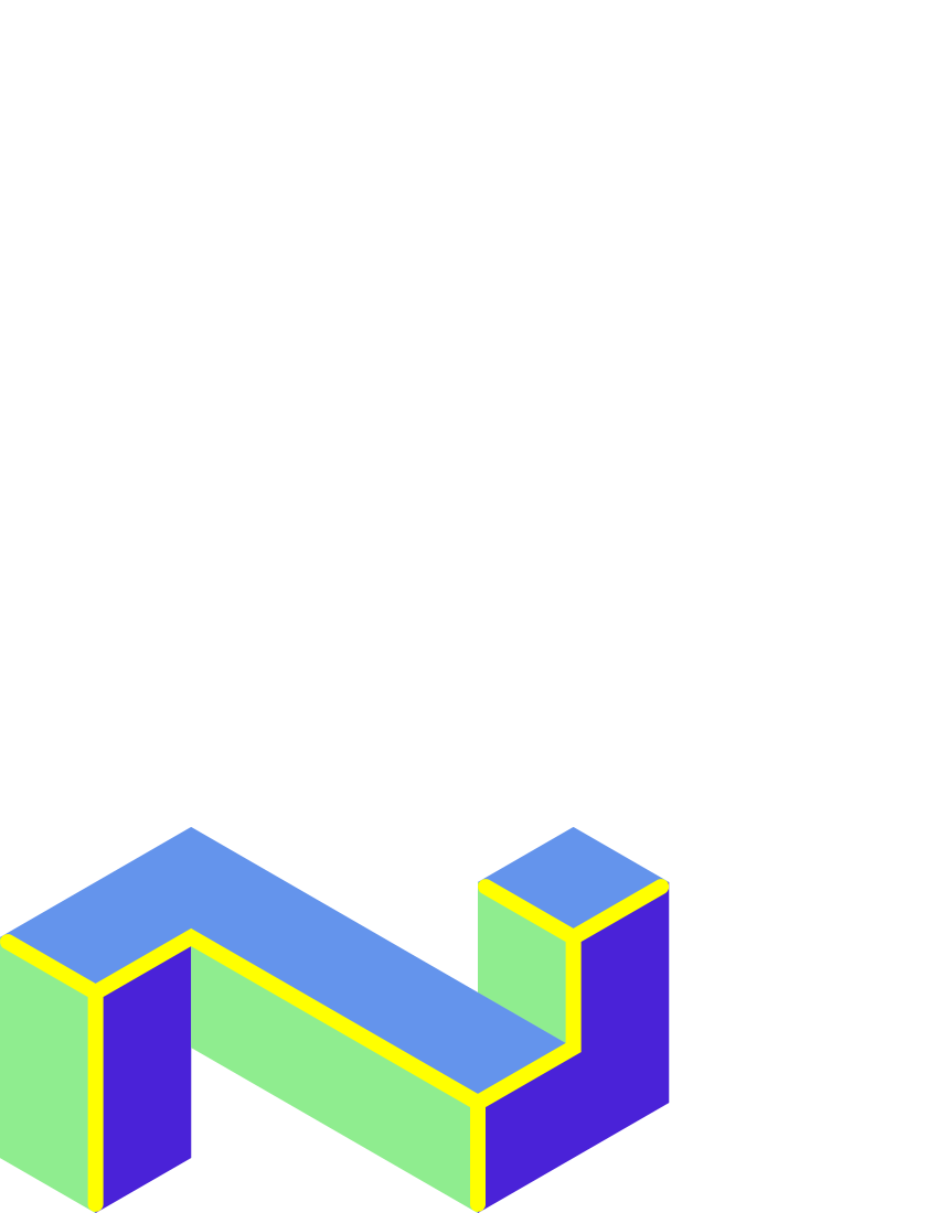
Figure 6: Surface enclosing the minimal volume

In the $c\to\pm\infty$ limit, the inscribed curve collapses to (a part of) the corner locus (locus where the surface is not smooth) of this piecewise linear surface, an example of which is plotted in yellow in Figure 6. The relevant parts of the corner locus are convex edges for volume maximizers and concave edges for minimizers (as seen from above the graph).

Our goal is to reverse this degeneration, that is, starting with the concave corner locus of the volume minimizing surface, we construct a certain tropical curve $Q_{T}$, the would-be dual of the inscribed curve. Then we show that $Q_{T}$ can be deformed to a rational degree $d$ winding curve $Q(x,y;c)=0$ whose dual curve $R(x,y;c)=0$ is inscribed in $\operatorname{\mathcal{E}xp}(\Omega)$ for all sufficiently large $c$. Finally, we prove that these curves can be further deformed to any finite value of $c$.

In order for the very first step to work, we need to assume that $\Omega$ is feasible, otherwise there is no volume maximizing surface to begin with. We further assume that $\Omega$ is generic, that is, there are no accidental relations between its side lengths. In particular, for generic $\Omega$, the triple points of the concave corner locus of the volume minimizers are local minima, see the illustration in Figure 7. Moreover, genericity implies that the maximizing surface lies strictly above the minimizing surface, except at the boundary. This implies that there are no “taut” paths, that is, paths in the interior which are present in every surface. See Figure 8 for an example of a taut path.

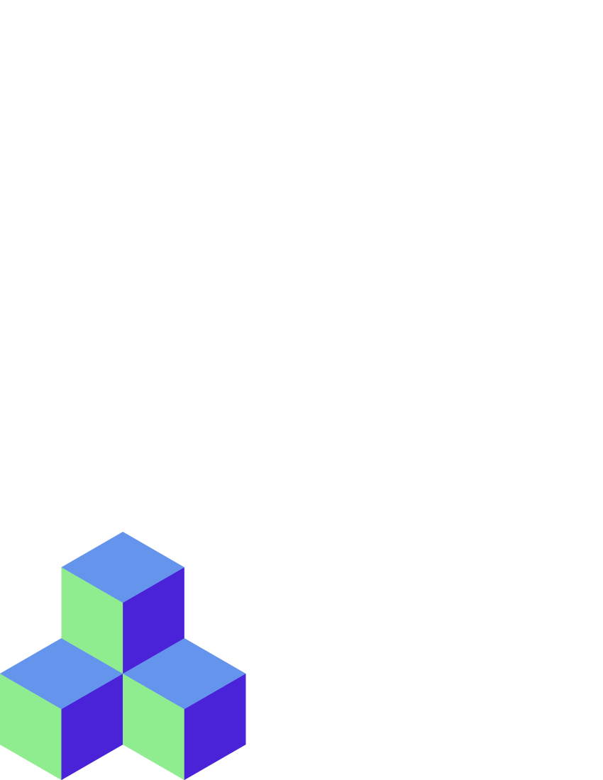
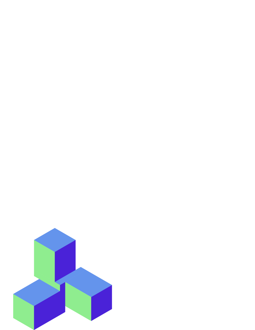
Figure 7: A nongeneric polygon $\Omega$ and a nearby generic one.

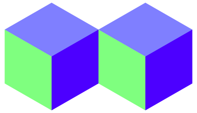
Figure 8: A polygon with a taut path (the vertical bisector). In a tiling, no tile crosses the taut path.

3.3.2 The tropical curve

The construction of the tropical curve is very simple: take the concave corner locus of the volume minimizer and extend univalent and 2-valent vertices to 3-valent ones as in Figure 9, where the newly added rays are shown in blue (thinner lines).

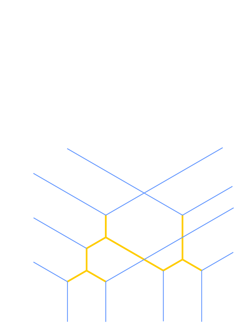
Figure 9: The tropical curve associated to the surface in Figure 6.

The tropical curve $Q_{T}$ thus obtained is a genus zero degree $d$ tropical hyperbolic curve, see [22] where properties of such curves are discussed in detail.

Consider the connected components of the complement of $Q_{T}$, which we will call chambers. There are $\binom{d+2}{2}$ chambers and they naturally correspond to lattice points in the triangle with vertices $(0,0)$, $(d,0)$ and $(0,d)$. The meaning of this triangle for us is that it is the Newton polygon of the degree $d$ curve $Q(x,y;c)$.

The dual of the graph $Q_{T}$ is, combinatorially, a tessellation of this triangle with unit size triangles and rhombi (recall that we assume $\Omega$ is generic). Each rhombus in the tessellation will correspond to a node of $Q(x,y;c)=0$; there will be $\binom{d-1}{2}$ of such.

Note that triple points of $Q_{T}$ come in two different orientations, and triple points of one of the two orientations correspond bijectively to local maxima of the concave corner locus.

3.3.3 Construction of $Q$

We will first construct an approximation

$$Q^{0}(x,y;c)=\sum_{i+j\leq d}q^{0}_{ij}\,x^{i}y^{j}\,,$$ (22)

to the true winding curve $Q$.

Recall that the monomials of $Q$ correspond to chambers of $Q_{T}$. For example, monomials that differ by a factor of $x$ correspond to adjacent chambers separated by a vertical line (which sometimes can have zero length). Let $x=\alpha_{ij}$ be the line separating the chambers corresponding to the monomials $x^{i}y^{j}$ and $x^{i+1}y^{j}$. Then we require that

$$\frac{q^{0}_{i+1,j}}{q^{0}_{i,j}}=e^{-c\alpha_{ij}}\,.$$

Similarly, for monomials that differ by factor of $y$, we set

$$\frac{q^{0}_{i,j+1}}{q^{0}_{i,j}}=e^{-c\beta_{ij}}$$

if the line separating the chambers is $y=\beta_{ij}$. For monomials which share a diagonal edge $x-y=\gamma_{ij}$ we have

$$\frac{q^{0}_{i,j+1}}{q^{0}_{i+1,j}}=e^{-c\gamma_{ij}}\,.$$

Since at a trivalent vertex we have

$$\beta_{ij}-\alpha_{ij}=\gamma_{ij},$$

this rule defines the curve $Q^{0}=0$ uniquely and unambiguously up to a common factor. The irrelevant common factor may be chosen so that all coefficients of $Q^{0}$ are real and positive.

By construction, as $c\to\infty$ the amoeba of the curve $Q^{0}$, scaled by $c$, converges to the tropical curve $Q_{T}$. In particular, $Q^{0}$ intersects the coordinate axes approximately at the points

$$(1,0,-e^{c\alpha_{i}}),\quad(0,1,-e^{c\beta_{i}}),\quad(1,-e^{-c\gamma_{i}},0)\,,$$ (23)

where

$$x=\alpha_{i},\quad y=\beta_{i},\quad x-y=\gamma_{i},\quad i=1,\dots,d\,.$$

are the lines forming the $3d$ sides of $\Omega$ By a small $c$-dependent change of the original curve $Q_{T}$, we can make the curve $Q^{0}$ defined by (22) pass precisely through the points (23).

A small deformation of a quadruple point of $Q_{T}$ (into a pair of triple points connected in one of two ways) leads to the change of the topology of the real locus of $Q^{0}$ for all large $c$. There is a $c$-dependent deformation of $Q_{T}$ for which every quadruple point becomes a real node, see [16]. Thus, for all $c\gg 0$, we have constructed a genus zero curve passing through the points (23). This is our curve $Q(x,y;c)$.

3.3.4 Intersections with lines

Our next step is to prove that the curve $Q(x,y;c)$ is winding. This involves understanding its real locus. We know that the curves

$$Q(\pm e^{cx},\pm e^{cy};c)=0$$ (24)

approach $Q_{T}$ as $c\to\infty$. One of these four curves, the one that corresponds to the $(+,+)$ choice of signs is empty because $Q$ has only positive coefficients. The shape of the other three curves can be inferred from simplest example of a conic, shown in Figure 10. The colors in Figures 10, 12 and 13 are explained in the following table:

quadrant	$(+,+)$	$(+,-)$	$(-,+)$	$(-,-)$
color	dotted	black	dashed	gray

The essential feature seen in Figure 10 is that the black and dashed curves cross over near the middle of the corresponding edge of the tropical curve. (Note that for clarity in some of the figures we use rectilinear coordinates and in others, coordinates with the $3$-fold symmetry. Hopefully these coordinate changes will not confuse the reader).

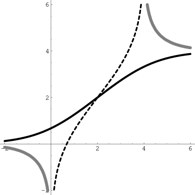
Figure 10: The curves $Q(\pm e^{x},\pm e^{y})=0$ for $Q(z,w)=1+z+w+e^{-4}zw$.

This same feature holds in general since for $c$ sufficiently large, the structure of the curves near a compact edge of $Q_{T}$ only depends on the coefficients of $Q$ corresponding to the four chambers around that edge: the other coefficients are exponentially small compared to these. It follows that the curves (24), in our running example, look like the curves in Figure 11.

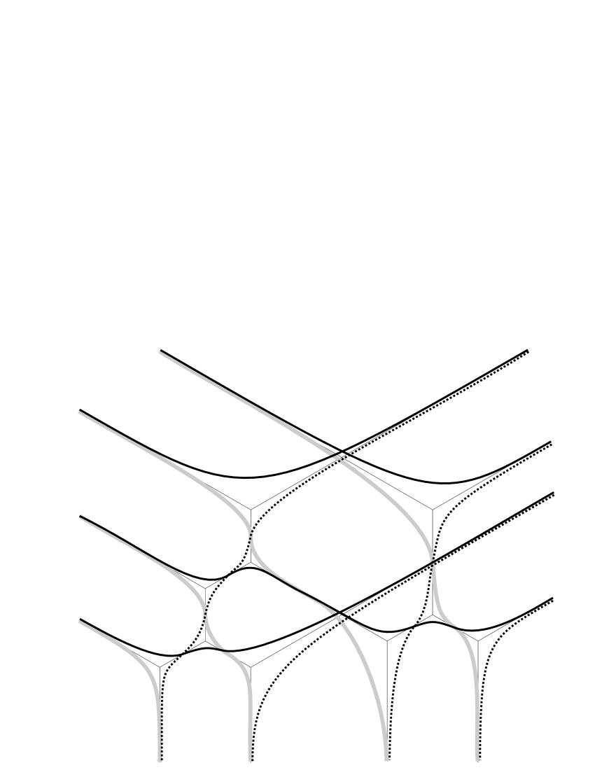
Figure 11: This is how the curves $Q(\pm e^{cx},\pm e^{cy};c)=0$ look like for $c\gg 0$ for the tropical curve in Figure 9.

Now we turn to intersecting the curves $Q(x,y;c)$ with lines. There are two kinds of lines, those that intersect the positive quadrant and those that don’t. The latter ones can be defined by an equation with positive coefficients. The difference between the two kinds of lines is illustrated in Figure 12. As we will see only lines that miss the positive quadrant have a chance to intersect $Q(x,y;c)$ in fewer than $d$ points.

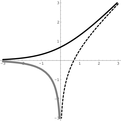
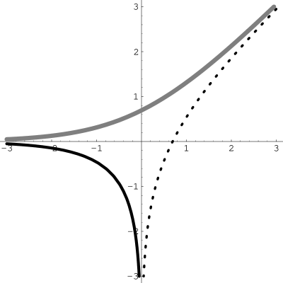
Figure 12: The curves $Q(\pm e^{x},\pm e^{y})=0$ for $Q(z,w)=1+z+w$ and $Q(z,w)=1-z+w$.

A basic property of any generic tropical curve, and of $Q_{T}$ in particular, is that it intersects a generic tropical line in $d$ points, where $d$ is the degree. Generic here means that the triple point of the line is not a point of the tropical curve. It is easy to see that in this generic situation there are still $d$ points of intersection of the nearby nontropical curve $Q$ with a nearby line: transverse intersections are preserved under deformations.

If a line is not generic, some of these points of intersection may be lost. Note that real points have to be lost in pairs, so, for example, if the triple point of the line lands on a (noncompact) ray of $Q_{T}$, there are still $d$ real points of intersection for nearby curves (this follows because the point at infinity has two colors for both $Q$ and the line and so this point is still a point of intersection). However, if the triple point of the line lands on a compact segment of $Q_{T}$, two points of intersection may disappear. If the triple point of the line lands on a triple point of $Q_{T}$ of the opposite orientation, two points of intersection (at most) may disappear. Finally, if the triple point of the line is a triple point of $Q_{T}$, with the same orientation, and all incident segments of $Q_{T}$ are compact, then as many as $4$ real points of intersection may be lost (Figure 13).

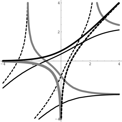
Figure 13: How to lose four intersections. The $Q$ curve here is in thinner colors, the line in thicker colors.

A simple but crucial observation is that, by construction, the curve $Q_{T}$ has no triple points of the same orientation as the tropical line and incident to 3 compact edges. This is because, as discussed earlier and illustrated in Figure 7, triple points of compact edges correspond to local minima of the volume minimizer for generic $\Omega$.

Furthermore, it is elementary to check that if the line intersects the positive quadrant then it has $d$ points of intersection with $Q$. Similarly, any tropical line with a triple point sufficiently far away from the amoeba of $Q_{T}$ meets $Q$ in $d$ points. Thus the curve $Q$ is winding.

The dual cloud curve $R=Q^{\vee}$, which, recall, is convex and non-sef-intersecting, is approximately the yellow convex corner locus from Figure 6. This is because the tropical lines whose triple points lie on a compact edge of $Q_{T}$ are exactly those which lead to fewer than $d$ points of intersection. The curve $R$ is inscribed in $\Omega$ because, if it were protruding it would have more, say, vertical tangents than we constructed. This is impossible since more than $d$ vertical tangents means more than $d$ points of intersection of $Q$ with a certain line.

3.3.5 Deforming the winding curve

We will now show that the inscribed curve that we constructed for $c\gg 0$ can be deformed to any given value of $c$. Changing $c$ produces a particular $1$-parameter family of polygons into which a cloud curve is to be inscribed. It is more convenient, in fact, to consider the general variation of the polygon $\operatorname{\mathcal{E}xp}(\Omega)$.

In the set of all polygons $\Omega$ with $3d$ disjoint edges (that is, no part of $\partial\Omega$ is traversed twice) consider the set of all feasible ones. Denote the interior of this feasible set by $\Upsilon$. Each connected component of $\Upsilon$ is naturally an open set of $\mathbb{R}^{3d-1}$. Let $\Upsilon_{0}\subset\Upsilon$ be the set of those $\Omega$ for which there exists an irreducible cloud curve $R$ without tacnodes inscribed in $\operatorname{\mathcal{E}xp}(\Omega)$ with $c=1$. Our goal is to prove that $\Upsilon_{0}=\Upsilon$.

We know that the intersection of $\Upsilon_{0}$ with each connected component of $\Upsilon$ is nonempty. In fact, if $\Omega$ is generic, then $c\Omega$, $c\gg 0$, is contained in $\Upsilon_{0}$.

Observe that $\Upsilon_{0}$ is open. This follows from Proposition 6 because changing $\Omega$ amounts to moving the points of intersection of $Q$ with the coordinate axes.

We claim that $\Upsilon_{0}$ is also closed. Indeed, let $\Omega$ be a limit point of $\Upsilon_{0}$. Since the set of winding curves is closed and $R$ remains bounded, there will be an inscribed cloud curve $R$ in $\operatorname{\mathcal{E}xp}(\Omega)$, but it might be reducible or tacnodal, or both. Since the map from $R$ to the circumscribed polygon is continuous, it is enough to show that the codimension $1$ degenerations cannot happen, that is, it is impossible to acquire exactly one tacnode or one extra node.

If the curve $R$ develops a tacnode this means that a part of the frozen region is swallowed by the liquid region as in Figure 14. This is impossible because, for example, there must be a point of tangency with the boundary between any two cusps of $R$.

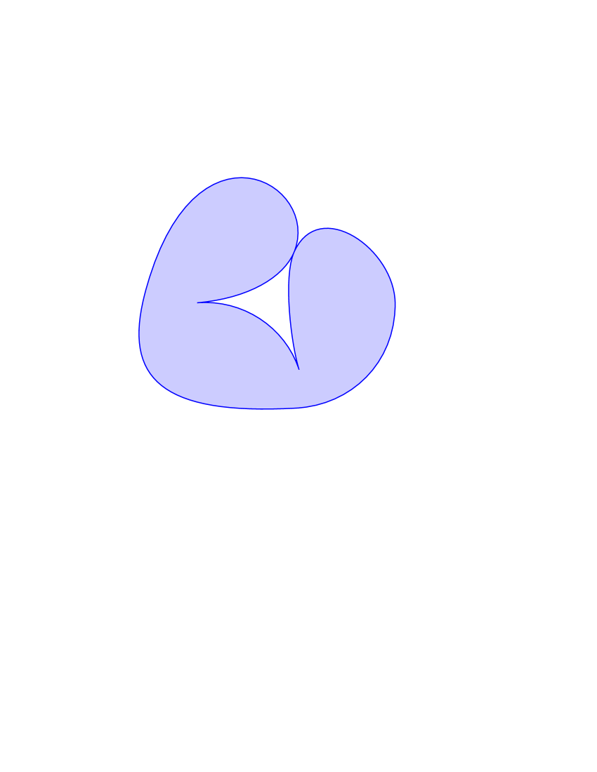
Figure 14: A cloud curve develops a tacnode

The other potential degeneration is when $Q$ develops an extra node (and, hence, becomes reducible). First suppose that neither component of the degenerate curve is a line. In this case, the dual curve $R$ becomes the union of two cloud curves and a double line tangent to both of them. Nearby cloud curves look like a union of the two disjoint cloud curves connected by a thin elliptical piece along a double tangent, see illustration in Figure 15 on the left. This, for example, is what happens if we squeeze the polygon in Figure 6 in the middle until the middle portion goes to zero width. This example, however, is not generic because the linear pieces of the limit shape on two sides of the collapsing ellipse have different slopes and meet along a line in a coordinate direction. Generically, the double tangent is not a line in a coordinate direction and these linear pieces (which then have the same slopes) merge together. This leads to a taut path in the polygon and, hence, cannot happen in our situation.

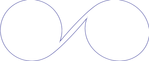
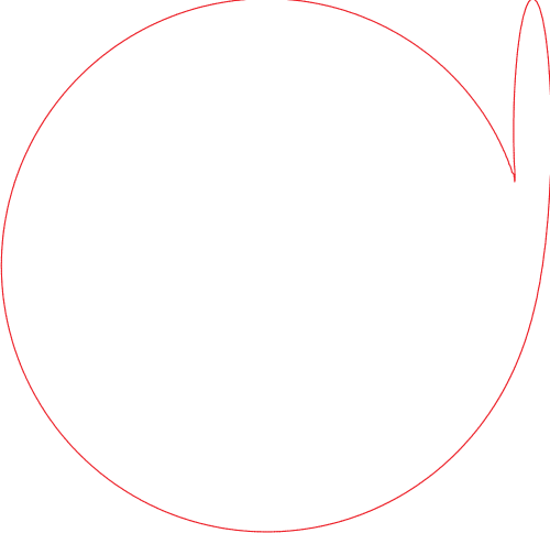
Figure 15: A cloud curve becomes reducible

The other possibility is when $Q$ degenerates to a union of a winding curve $Q_{1}$ and a line $Q_{2}$. The line $Q_{2}$ corresponds to a point $p_{2}$ of the dual plane and the collapsing ellipse follows the tangent from $p_{2}$ to $Q^{\vee}_{1}$, this is illustrated in Figure 15 on the right. This degeneration can only happen if an edge of $\Omega$ has length tending to zero.

Note that in codimension two one can have a degeneration in which two cusps of the frozen boundary come together and merge in a tacnode, reminiscent of the Henry Moore’s Oval with Points. This corresponds in Figure 15, left part, to the thin ellipse having zero size.

Finally, there is practical side to the above deformation argument. Namely, it allows us to find the inscribed curve by numeric homotopy, that is, by solving the equations using Newton’s algorithm with the solution of the nearby problem as the starting point. An example of a practical implementation of this can be see in Figure 16.

Figure 16: Frozen boundaries (at $c<0,c=0$ and $c>0$) for the polygonal region in Figure 6.

3.3.6 Uniqueness

It remains to prove that the inscribed curve is unique and that the polygon is feasible if the inscribed curve exists. Given the inscribed curve $R$, let $h^{\star}$ denote the height function obtained from it by the procedure of Section 1.8. This is a well-defined function with gradient in the triangle (1). Therefore $\Omega$ is feasible. The inscribed curve is unique because by the results of Sections 3.3.5 it has a unique deformation to the unique tropical inscribed curve.

4 Global minimality

As before, let $h^{\star}$ denote the height function constructed from the inscribed cloud curve $R$.

Theorem 4.

The height function $h^{\star}$ is the unique minimum for the variational problem (4).

Proof.

By strict convexity of the surface tension, there is a unique minimizer. Therefore we need to prove that

$$\mathcal{E}(g)\geq\mathcal{E}(h^{\star})$$ (25)

for any function $g$ satisfying the boundary conditions and with gradient in (1). Since the integrand in (4) is bounded, we can freely modify it on sets of arbitrarily small measure. In particular, it is enough to prove (25) for functions $g$ such that $g=h^{\star}$ in a neighborhood of the vertices of $\Omega$.

For any such $g$, we will construct a sequence $\{h_{n}\}$ converging to $h$ such that

• $\mathcal{E}(h_{n})\to\mathcal{E}(h^{\star})$, as $n\to\infty$ ,

• $\mathcal{E}$ has a directional derivative at $h_{n}$ in the direction of $g-h_{n}$ ,

• this directional derivative is nonnegative for all $n\gg 0$  .

By convexity of $\mathcal{E}$, the last condition implies that $\mathcal{E}(g)\geq\mathcal{E}(h_{n})$ for all $n\gg 0$, from which (25) follows.

Now we proceed with the construction of the sequence $\{h_{n}\}$. In the liquid region we will take $h_{n}=h^{\star}$, except in a very thin strip along the frozen boundary. Inside the facet, $h_{n}$ will be a smooth function very slightly deviating from $h^{\star}$ and equal to it in a fixed neighborhood of the vertices of $\Omega$. Note that the facets of $h^{\star}$ are of two types: the “bottom” facets, for which $g\geq h^{\star}$ for any allowed function $g$, and the “top” facets, where the inequality is reversed. For example, the bottom facet in Figure 1 is also a bottom facet according to the above definition. For concreteness, we will give a construction of $h_{n}$ on a bottom facet; the case of a top facet is the same, with obvious modifications.

The construction of Section 3.3 give a family of solutions of the Euler-Lagrange equation (3) parameterized by a real constant $c$. Since we will need all of them for the argument that follows, we will use $c_{0}$ to denote the particular value of the Lagrange multiplier in (4) for which we wish to prove that $h^{\star}$ is a minimizer. Note that the height at any point is a decreasing function of $c$. Indeed, the $c$-derivative $\phi=\frac{\partial h^{\star}}{\partial c}$ of the height function solves the linearization of (3), which has the form

$$\operatorname{div}G\cdot\nabla\phi=1\,,$$

with a positive definite matrix $G=\nabla^{2}\sigma(\nabla h^{\star})$ in the liquid region and zero boundary conditions on the frozen boundary. The condition $G\geq 0$ guarantees $\phi$ has no local maxima and hence $\phi\leq 0$.

Consider a horizontal bottom facet of $h^{\star}$. Its boundary is formed by a part of $\partial\Omega$ and a part of the frozen boundary. Let us denote that part of the frozen boundary $F_{c_{0}}$ and call it the frozen front. For $c$ below $c_{0}$, the monotonicity $\frac{\partial h^{\star}}{\partial c}\leq 0$ implies the frozen front $F_{c}$ moves inside the facet. It sweeps the entire facet as $c\to-\infty$.

By our assumption on $g$, we can find $C\ll 0$ such that $g=h^{\star}$ outside $F_{C}$. The functions $h_{n}$ will smoothly interpolate between $h^{\star}$ outside $F_{C}$ and $h^{\star}$ just inside $F_{c_{0}}$ in such a way that

$$0<\|\nabla h_{n}\|<_{\textup{ess}}O(n^{-1/2})\,,\quad n\to\infty\,.$$

between $F_{C}$ and $F_{c_{0}}$. Here $<_{\textup{ess}}$ means that the inequality is satisfied except on a set whose measure goes to zero as $n\to\infty$.

The derivative of $\mathcal{E}$ at $h_{n}$ in the direction $g-h_{n}$ equals

$$\int(c-\operatorname{div}\nabla\sigma(\nabla h_{n}))\,(g-h_{n})\,,$$

which is nonnegative for all sufficiently large $n$ provided $g>h^{\star}$ somewhere on the facet and

$$\operatorname{div}\nabla\sigma(\nabla h_{n})\leq c$$

between $F_{C}$ and $F_{c_{0}}$.

The functions $h_{n}$ will be obtained by patching together solutions of

$$\operatorname{div}\nabla\sigma(\nabla f_{i})=c_{i}\,,$$ (26)

where

$$c=c_{0}>c_{1}>c_{2}>c_{3}>\dots>c_{n}=C\,,$$

are chosen so that all the distances between the fronts $F_{c_{i}}$ go to zero as $O(n^{-1})$ as $n\to\infty$. The implicit constants in $O(\dots)$ here and below are bounded in terms of $C$.

For each $c_{i}$, consider the algebraic solution $f_{i}$ of (26) with frozen front $F_{c_{i}}$. Since near the frozen boundary its gradient has a square root growth, we have $\|\nabla f_{i}\|=O(n^{-1/2})$ between $F_{c_{i}}$ and $F_{c_{i-1}}$. This means that the discontinuous surface formed by the union of $f_{i}$’s between $F_{c_{i}}$ and $F_{c_{i-1}}$ is nearly flat for $n\gg 0$. To make it continuous, we shift each successive piece slightly in the $x_{3}$ direction (recall that our facet is assumed to be horizontal) and insert a smooth nearly vertical strip of surface between two $f_{i}$’s. The width of each of these strips is $O(n^{-3/2})$ and so their contribution to the functional is negligible. There will be also a small region near the boundary of $\Omega$ where $f_{i}$ is not defined. Since each $F_{c_{i}}$ is tangent to $\partial\Omega$, the area of that region is $O(n^{-3})$ and so we can extend $f_{i}$ there as an arbitrary smooth Lipschitz function. Thus we have constructed the required sequence $\{h_{n}\}$. ∎

5 Explicit examples

In this section we work out some explicit solutions to (10) for various cases.

It can be checked along the lines of Section 4 that the solutions we construct below are minimizers for their corresponding variational problem.

5.1 Disconnected boundary example

The simplest multiply-connected regions are obtained from simply-connected regions by removing points. In this case the inner boundary components are reduced to points and specifying a surface with these boundary conditions is equivalent to specifying the height of the surface at given points in the interior of the domain.

Figure 17 shows an example: here the outer contour is a hexagon ($6$ edges of a cube) and the inner contour is a single point, the central point in the figure, located at a height which is $2/3$ of the way between the upper and lower vertices of the corresponding cube.

The curve $Q$ is a cubic curve which by symmetry has the form

$$Q(z,w)=\begin{array}[]{llll}w^{3}\\ +bw^{2}&+bzw^{2}\\ +bw&+azw&+bz^{2}w\\ +1&+bz&+bz^{2}&+z^{3}.\end{array}$$

The coefficient $b$ is determined by the intersection of $Q$ with coordinate axes, that is, it determined by the size of the cube and the value of Lagrange multiplier $c$. The coefficient $a$ determines the height of the central point.

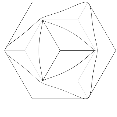
Figure 17: Boxed plane partition conditioned to pass through a given point. The gray edges lie below the surface.

5.2 Example with a bubble

In this section we consider dimers on the square-octagon graph. Here $P(z,w)=5+z+1/z+w+1/w$, see [13]. The Newton polygon is defined by $|x|+|y|\leq 1$. Consider the contour $C$ through the points

$$(1,0,0),(0,1,1),(-1,0,0),(0,-1,1)\,,$$

see Figure 18.

We expect $4$ frozen phases and hence $4$ points where the frozen phases change along the frozen boundary. Such points correspond to points of $P$ at the toric infinity, that is, tips of tentacles of the amoeba of $P$. We, therefore, expect $Q$ to have the same Newton polygon as $P$. From symmetry, we conclude that

$$Q(z,w)=b+z+1/z+a(w+1/w)\,.$$

The point $(z,w)=(\infty,\infty)$ on $P$ occurs somewhere along the upper right boundary edge (the line $x+y=1$) since this is the point of separation of the two adjacent frozen phases. Eliminating $w$ using (10), substituting $y=1-x$, and expanding near $z=\infty$ gives

$$a=e^{-c+2cx_{0}}\,,\quad b=5e^{-2c+3cx_{0}}\,,$$

where $(x_{0},1-x_{0})$ is the point of intersection of the frozen boundary with the line $x+y=1$. This leaves us with one variable, $x_{0}$, which is determined by the area constraint from Proposition 4.

While it is a non-trivial computation to compute $x_{0}$ in general, in the case $c=0$ we have an extra symmetry and expect $x=1/2$. This leads to a degree $8$ equation

$$729-13608x^{2}-22896x^{4}+64000x^{6}+102400x^{8}-13608y^{2}+\\ 412992x^{2}y^{2}-1104000x^{4}y^{2}+870400x^{6}y^{2}-22896y^{4}-1104000x^{2}y^{4}+\\ 2054400x^{4}y^{4}+64000y^{6}+870400x^{2}y^{6}+102400y^{8}=0$$ (27)

for the frozen boundary in the unconstrained volume case–see Figure 18. This was called the “octic circle” by Cohn and Pemantle [2].

This case can be obtained more simply using (9): there let $Q_{0}(z,w)\equiv-3/2$. We solve

$$P(z,w) = 0$$

$$-\frac{3}{2} = xzP_{z}+ywP_{w}$$

for $z,w$ as a function of $x,y$. The double root of these equations occurs along (27), as one immediately checks using resultants.

Figure 18: frozen boundaries for the square-octagon “fortress” example.

5.3 Crystal corner boundary conditions

In this section we consider minimizers defined on the whole plane and satisfying piece-wise linear boundary conditions at infinity. They can be interpreted as dissolution shapes of an infinitely large crystal near one of its corners.

5.3.1 Minkowski sums of Ronkin functions

Recall that the Minkowski sum of two sets $A,B\in\mathbb{R}^{n}$ is

$$A+B=\{x+y~{}|~{}x\in A,~{}~{}y\in B\}.$$

If $A$ and $B$ are convex, so is their sum.

For a curve $Q(z,w)$ let $A_{Q}$ be the set of points in $\mathbb{R}^{3}$ lying on or above the graph of the Ronkin function $\mathcal{R}_{Q}$ of $Q$. This is a convex set.

A general class of solutions to the volume-constrained minimization problem for an arbitrary spectral curve $P$ can be constructed as follows.

Theorem 5.

Let $P^{\prime}$ be a Harnack curve with the same Newton polygon as $P$ such that the areas of the corresponding (compact) facets of $\mathcal{R}_{P}$ and $\mathcal{R}_{P^{\prime}}$ are equal. Then the boundary of the Minkowski sum of the sets $A_{P}$ and $A_{P^{\prime}}$ is a minimizer.

Proof.

It is a simple geometric property of the Minkowski sum that a facet on the boundary of $A_{P}+A_{P^{\prime}}$ is the Minkowski sum of a facet of $A_{P}$ and a facet of $A_{P^{\prime}}$ having the same slopes, where one of these facets may be reduced to a point. Any point $p$ on the boundary of $A_{P}+A_{P^{\prime}}$ but not on a facet is the sum of unique points on the boundary of $A_{P}$ and $A_{P^{\prime}}$ with tangent planes in the same direction.

Given a point $(x_{1},y_{1},\mathcal{R}_{P}(x_{1},y_{1}))$ on the graph of $\mathcal{R}_{P}$, which is not in the interior of a facet of $\mathcal{R}_{P}$, there is a corresponding point $(z_{1},w_{1})$ on the curve $P$, with $\log|z_{1}|=x_{1}$ and $\log|w_{1}|=y_{1}$, and such that the arguments of $z_{1}$ and $w_{1}$ are linearly related to the slope of $\mathcal{R}_{P}$ at $(x_{1},y_{1})$. The point $(x_{2},y_{2},\mathcal{R}_{P^{\prime}}(x_{2},y_{2}))$ with the same slope on the graph of $\mathcal{R}_{P^{\prime}}$ (and if this point is on the boundary of a facet, it must also have the same slope along the facet boundary as the corresponding point of $\mathcal{R}_{P}$) yields a corresponding point $(z_{2},w_{2})$ lying on the curve $P^{\prime}$ and with the same arguments.

Let $Q(z,w)=P^{\prime}(1/z,1/w)$. Construct the minimizer using the curve $Q$ in (10). Since $Q(e^{-cx}z_{1},e^{-cy}w_{1})=0$, we have $(z_{2},w_{2})=(e^{cx}/z_{1},e^{cy}/w_{1})$. Therefore

$$(x_{2},y_{2})=(\log|z_{2}|,\log|w_{2}|)=\\ (cx-\log|z_{1}|,cy-\log|w_{1}|)=c\cdot(x,y)-(x_{1},y_{1})\,,$$

and so $(x,y)=\frac{1}{c}((x_{1},y_{1})+(x_{2},y_{2}))$.

The scaled Minkowski sum is the unique shape whose tangent plane above $(cx,cy)$ has the same slope as the tangent planes at $(x_{1},y_{1})$ and $(x_{2},y_{2})$. Therefore it is the solution to the minimization problem (10), except that it may not satisfy the area constraints of Proposition 4. Those say precisely that the facet areas are equal. ∎

In [11] we proved that, for fixed boundary behavior, there is a unique Harnack curve with facets of given areas. So we can always find $P^{\prime}$ with the appropriate facet areas.

Note that if the facet areas of $P$ and $P^{\prime}$ do not match, we still get a $C^{3/2}$ function that solves the Euler-Lagrange equation in the liquid region and is locally a minimizer inside each facet. It is not a global minimizer since raising or lowering a facet as a whole will reduce the total surface tension. From the point of view of Glauber dynamics on random surfaces, moving the facet as a whole is an extremely slow process, so this solution of the Euler-Lagrange equation may be described as metastable.

Note also the symmetry between $P$ and $P^{\prime}$: $A_{P}+A_{P^{\prime}}$ is a minimizer for the variational problems for both $P$ and $P^{\prime}$.

There exist intriguing connections, first noticed in [19], between the random surfaces studied in this paper and topological sting theory, see e.g. [18] for a review aimed at mathematicians. In this context, the Minkowski sum construction has a natural interpretation which will be explained in [12].

5.3.2 Wulff construction

Taking $P^{\prime}=P$ in Theorem 5, we have $A_{P}=A_{P^{\prime}}$ and the facets trivially have the same area. So limit shape is a copy of the Ronkin function of $P$. This shows that the Ronkin function itself is a solution to the volume-constrained surface-tension minimization problem. Indeed, this is the classical Wulff construction, since the Ronkin function is the Legendre dual of the surface tension [13].

5.3.3 Higher-degree solutions

To combine $P$ with higher-degree curves in Theorem 5, one can take covers of $P$ as described in [13]: the curves

$$P_{n}=\prod_{\eta^{n}=\xi^{n}=1}P(\eta z^{1/n},\xi w^{1/n})$$

have the same Ronkin function up to scale as $P$, and $N(P_{n})=nN(P)$, where $N(P)$ stands for the Newton polygon of $P$.

Let $Q$ be a Harnack curve with $N(Q)=N(P_{n})$, and having facets of the same area as $P_{n}$. Then $A_{P_{n}}+A_{Q}$ is a scaled minimizer for $P_{n}$, and since $\sigma_{P_{n}}(ns,nt)=\sigma_{P}(s,t)$, $A_{P_{n}}+A_{Q}$ is also a scaled minimizer for $P$.

This allows us to combine $P$ with arbitrarily high-degree Harnack curves, and in fact by taking limits one can construct explicit non-algebraic minimizers.

5.3.4 Rational curves

A particular case of Theorem 5 is when $P$ has genus zero—then $Q$ must also have genus zero. Suppose $P(z,w)=z+w+1$. Then $P_{n}$ can be parameterized via $z\mapsto(z^{n}:(-1-z)^{n}:1)$. A degree-$n$ rational Harnack curve $Q$ has a parametrization

$$u\mapsto\left(A\prod_{i=1}^{n}(u-a_{i}):B\prod_{i=1}^{n}(u-b_{i}):C\prod_{i=1}^{n}(u-c_{i})\right)$$

with $A,B,C\in\mathbb{R}$ and where the real numbers $a_{1},\dots,a_{n},b_{1},\dots,b_{n},c_{1},\dots,c_{n}$ occur in cyclic order around $\mathbb{R}\cup\infty$ (that is, all the $a$’s come first, then the $b$’s and then the $c$’s), see [11].

Then (10) gives

$$z^{n} = e^{cx}\frac{C}{A}\prod_{i=1}^{n}\frac{u-c_{i}}{u-a_{i}}$$

$$(-1-z)^{n} = e^{cy}\frac{C}{B}\prod_{i=1}^{n}\frac{u-c_{i}}{u-b_{i}}.$$

The constants $c,A,B,C$ can be incorporated into an overall scale and translation. Suppose that as $n\to\infty$, the measures

$$\frac{1}{n}\sum\delta_{a_{i}}\,,\quad\frac{1}{n}\sum\delta_{b_{i}}\,,\quad\frac{1}{n}\sum\delta_{c_{i}}$$

have weak limits that we will denote by $d\mu_{i}$, $i=1,2,3$. Taking logarithms and limit, we find that the triangle discussed in Section 1.8 takes the form

$$\sum_{i=1}^{3}e^{c_{0}x_{i}+c_{i}}\exp\left(-\int\log(u-t)d\mu_{i}(t)\right)=0\,,$$ (28)

for certain constants $c_{0},\dots,c_{3}$.

References

- [1] A. Abanov, Hydrodynamics of correlated systems. Emptiness Formation Probability and Random Matrices, Applications of random matrices in physics, 139–161, NATO Sci. Ser. II Math. Phys. Chem., 221, Springer, Dordrecht, 2006. cond-mat/0504307.
- [2] H. Cohn, R. Pemantle, unpublished, communicated to the authors.
- [3] H. Cohn, R. Kenyon, J. Propp, A variational principle for domino tilings, J. Amer. Math. Soc., 14(2001), no. 2, 297-346.
- [4] Ph. Griffiths and J. Harris, Principles of Algebraic Geometry, John Wiley & Sons, New York, 1994.
- [5] A. Guionnet, First order asymptotics of matrix integrals; a rigorous approach towards the understanding of matrix models, Comm. Math. Phys. 244 (2004), no. 3, 527–569.
- [6] J.-C. Fournier, Pavage des figures planes sans trous par des dominos: fondement graphique de l’algorithme de Thurston et parallélisation, Compte Rendus del L’Acad. des Sci., Serie I 320 (1995), 107–112.
- [7] W. Fulton and R. Pandharipande, Notes on stable maps and quantum cohomology, Algebraic geometry—Santa Cruz 1995, 45–96, Proc. Sympos. Pure Math., 62, Part 2, AMS, Providence, RI, 1997.
- [8] J. Harris and I. Morrison, Moduli of curves, Springer, 1998.
- [9] I. Itenberg and O. Viro, Patchworking algebraic curves disproves the Ragsdale conjecture, Math. Intelligencer 18 (1996), no. 4, 19–28.
- [10] R. Kenyon, Height fluctuations in honeycomb dimers, math-ph/0405052.
- [11] R. Kenyon, A. Okounkov, Dimers and Harnack curves, Duke Math. J. 131 (2006), no. 3, 499-524.
- [12] R. Kenyon, A. Okounkov, C. Vafa, in preparation.
- [13] R. Kenyon, A. Okounkov, S. Sheffield, Dimers and Amoebae, Annals of Math. 163 (2006), no.3, 1019-1056.
- [14] A. Matytsin, On the large- limit of the Itzykson-Zuber integral Nuclear Phys. B 411 (1994), no. 2-3, 805–820.
- [15] G. Mikhalkin, Amoebas of algebraic varieties and tropical geometry, Different faces of geometry, 257–300, Int. Math. Ser., Kluwer/Plenum, New York, 2004, math.AG/0403015.
- [16] G. Mikhalkin, Enumerative tropical algebraic geometry in , J. Amer. Math. Soc. 18 (2005), no. 2, 313–377
- [17] Ch. Morrey, Jr., Multiple integrals in the calculus of variations, Die Grundlehren der mathematischen Wissenschaften, Band 130, Springer-Verlag New York, Inc., New York 1966.
- [18] A. Okounkov, Random surfaces enumerating algebraic curves, European Congress of Mathematics, 751–768, Eur. Math. Soc., Z rich, 2005.
- [19] A. Okounkov, N. Reshetikhin, C. Vafa, Quantum Calabi-Yau and Classical Crystals, The unity of mathematics, 597–618, Progr. Math., 244, Birkh user Boston, Boston, MA, 2006.
- [20] M. Passare and H. Rullgård, Amoebas, Monge-Amp re measures, and triangulations of the Newton polytope, Duke Math. J. 121 (2004), no. 3, 481–507.
- [21] V. Pokrovsky, A. Talapov, Theory of two-dimensional incommensurate crystals, JETP (Zhurnal Experimentalnoi i Teoreticheskoi Fiziki), 78 (1980), no. 1, 269-295.
- [22] D. Speyer, Horn’s Problem, Vinnikov Curves and the Hive Cone, Duke Math. J. 127 (2005), no. 1, 395-427.
- [23] V. Vinnikov, Selfadjoint determinantal representations of real plane curves, Math. Ann. 296 (1993), no. 3, 453–479.